large-eddy simulations of radiatively driven …€¦ · large-eddy simulations of radiatively...

1 DECEMBER 1999 3963S T E V E N S E T A L .

q 1999 American Meteorological Society

Large-Eddy Simulations of Radiatively Driven Convection: Sensitivities to theRepresentation of Small Scales

BJORN STEVENS, CHIN-HOH MOENG, AND PETER P. SULLIVAN

National Center for Atmospheric Research,* Boulder, Colorado

(Manuscript received 20 February 1998, in final form 10 February 1999)

ABSTRACT

Large-eddy simulations of a smoke cloud are examined with respect to their sensitivity to small scales asmanifest in either the grid spacing or the subgrid-scale (SGS) model. Calculations based on a Smagorinsky SGSmodel are found to be more sensitive to the effective resolution of the simulation than are calculations basedon the prognostic turbulent kinetic energy (TKE) SGS model. The difference between calculations based on thetwo SGS models is attributed to the advective transport, diffusive transport, and/or time-rate-of-change termsin the TKE equation. These terms are found to be leading order in the entrainment zone and allow the SGSTKE to behave in a way that tends to compensate for changes that result in larger or smaller resolved scaleentrainment fluxes. This compensating behavior of the SGS TKE model is attributed to the fact that changesthat reduce the resolved entrainment flux (viz., values of the eddy viscosity in the upper part of the PBL)simultaneously tend to increase the buoyant production of SGS TKE in the radiatively destabilized portion ofthe smoke cloud. Increased production of SGS TKE in this region then leads to increased amounts of transported,or fossil, SGS TKE in the entrainment zone itself, which in turn leads to compensating increases in the SGSentrainment fluxes. In the Smagorinsky model, the absence of a direct connection between SGS TKE in theentrainment and radiatively destabilized zones prevents this compensating mechanism from being active, andthus leads to calculations whose entrainment rate sensitivities as a whole reflect the sensitivities of the resolved-scale fluxes to values of upper PBL eddy viscosities.

1. Introduction

In this paper we report on a series of large-eddy sim-ulations (LES) of an idealized PBL driven by radiativecooling from the top of a radiatively opaque layer offluid—a smoke cloud. The purpose of our study is toexplore and understand the sensitivity of LES to smallscales, as manifest in either the resolution of the meshor the model of subgrid-scale (SGS) motions. Thesmoke cloud is studied because we find that it retainssensitivities that we have also found to be evident insimulations of stratocumulus (Stevens et al. 1998) andbecause by only representing the essential features ofradiatively driven stratocumulus, without the compli-cations associated with the generation or consumptionof latent heat through cloud microphysical processes(e.g., Lilly 1968; Moeng and Schumann 1991; Breth-erton et al. 1999), it is somewhat simpler.

* The National Center for Atmospheric Research is sponsored bythe National Science Foundation.

Corresponding author address: Mr. Bjorn Stevens, Dept. of At-mospheric Sciences, University of California, Los Angeles, Los An-geles, CA 90095.E-mail: [email protected]

The smoke cloud PBL that we consider in this paperis the one proposed by Bretherton et al. (1999). A com-plicating, albeit realistic and physically interesting,characteristic of this experiment, as opposed to a typicalclear convective boundary layer (CBL), is that the de-gree of stable stratification between the turbulent andquiescent layers is large when compared to the vigor ofthe underlying turbulence. Typically this aspect of theflow is measured in terms of a bulk Richardson number(e.g., Deardorff et al. 1980; Turner 1986), RiB:

gz DQiRi 5 , (1)B 2Q w0 s

where zi is the depth of the turbulent layer, DQ char-acterizes the temperature jump between the two layers,ws is a scale velocity characterizing the turbulent fluid,and g/Q0 is the ratio of gravity to a reference temper-ature.1 In the smoke cloud experiment RiB . 200; such

1 RiB is similar to the inverse of the square of the bulk FroudeNumber as earlier defined by Rouse and Dodu (1955). If the ge-neric scale velocity used in Eq. (1) is replaced by Deardorff ’sconvective scale velocity, then our RiB is identical to Deardorff ’sRi

*. For most definitions of a Q

*(the convective temperature

scale), RiB 5 DQ/Q*

.

3964 VOLUME 56J O U R N A L O F T H E A T M O S P H E R I C S C I E N C E S

FIG. 1. Heat flux from LES showing the relationship between theentrainment heat flux and the extrapolated heat flux used in processpartitioning parameterizations of entrainment.

large values of RiB are typical of stratocumulus but morethan an order of magnitude greater than what is com-monly found in the CBL. One reason for this is that, incontrast to the CBL, in radiatively driven convectionthe driving force of the turbulence, that is, cooling ofair at cloud top, cooperates with turbulent processes topromote the development of sharp strong inversions.Sharp, strong inversions across which fluxes divergesignificantly are often difficult to resolve and thus posespecial numerical difficulties. But because sharp, stronginversions are common in stratocumulus boundary lay-ers that have been frequently studied with LES, we areinterested in understanding, in some generic sense, thebehavior of LES under such conditions.

The smoke cloud has recently come under intensestudy using both LES and laboratory analogs, and re-sults now emerging in the literature are somewhat inconflict. A key result of the laboratory work is that forsuch high RiB flows, the nondimensional entrainmentrate is a function of the Prandtl number of the fluid(Sayler and Breidenthal 1998). The interpretation of thisresult is that entrainment across the strongly stratifiedinterface, which separates the turbulent fluid from thequiescent fluid, depends on the diffusive thickening(through molecular processes) of the stratified layer, thatis, Taylor layers. The conclusion that the thickness ofthe Taylor layers regulates the entrainment rates in highRiB flows is troubling for LES, which by nature assumesthat molecular processes are inconsequential. Just howtroubling this is remains uncertain, mostly because thelaboratory results can be questioned on many grounds:they are low Reynolds number, the low aspect ratio ofthe container may bias the problem, container scale cir-culations may affect physical processes, and differencesin how the radiative forcing is applied may affect theanalogy between the laboratory flow and the LES. Thus,despite the fact that the laboratory experiments representa real flow, it is not obvious that such experiments areany better at representing the hypothetical smoke cloudthan is LES.

LESs of the smoke cloud are not only in conflict withthe low Reynolds number laboratory data, they alsodisagree among themselves. While there is generalagreement that fine vertical resolution is needed to prop-erly represent processes at the entrainment interface(e.g., Bretherton et al. 1999; Stevens and Bretherton1999; Lewellen and Lewellen 1998; Lock and MacVean1999; vanZanten et al. 1999; also see section 2 andappendix C of this article), there is disagreement as tothe importance of small-scale turbulence as manifest insensitivities to horizontal resolution or SGS model as-sumptions.2 For instance, simulations by the Lawrence

2 In discussions of LES results we often use the words small scalesto refer to scales on the order of the grid scale, which is orders ofmagnitude larger than the viscous or diffusive scales postulated tobe important in low Reynolds number high RiB laboratory flows.

Berkeley Labs–University of Washington (LBL–UW)group (Stevens and Bretherton 1999) display an explicitsensitivity to the horizontal resolution for weakly strat-ified experiments (small RiB); in contrast, simulationsby the West Virginia University (WVU) group (Lew-ellen and Lewellen 1998) are remarkable in their lackof sensitivity to horizontal resolution even for stronglystratified interfaces (large RiB). Thus while the range ofresolved scales appears to be important in determiningthe entrainment rate in the LBL–UW LES, this is notthe case for the LES by the WVU group.

Further disagreement among LES is also evident inrecently published entrainment relationships (Lewellenand Lewellen 1998; Lock and MacVean 1999; van-Zanten et al. 1999). Both the Lewellen and Lewellenand the vanZanten et al. studies have proposed that pro-cess partitioning provides a rational framework for de-scribing entrainment rates deduced from LES. Roughlyspeaking, for the smoke cloud this closure assumptioncan be interpreted as stating that the extrapolated buoy-ancy flux in an entraining PBL (denoted by ‘‘b’’ in Fig.1) is a fixed fraction of what it would be in the absenceof entrainment. In other words, process partitioning clo-sures predict that b/(a 1 b) or simply a/b is a universalconstant. Although calculations by a number of groupssuggest that their respective simulations are well con-strained by such a relationship, the entrainment relationsare, to a certain extent, model dependent. For instance,the IMAU (vanZanten et al. 1999) and the WVU (Lew-ellen and Lewellen 1998) groups predict a/b ø 0.4,while the UKMO group (Lock and MacVean 1999) pre-dicts a/b closer to 0.2. Scatter in the relationships amongthe models tends to be larger than the scatter associatedwith any one model, which suggests that the precision


TABLE 1. Initial sounding. In all cases the mean wind and all surfacefluxes are set to zero.

Height u s

0.0687.5712.5

2212.5

288.000288.000295.000295.156

1.01.00.0.

of an individual simulation is much greater than its ac-curacy.

Thus recent studies raise many questions: Do the en-trainment relationships found by various groups to de-scribe the behavior of large RiB flows reflect real phys-ical relationships? If so, what is the physical characterof these relationships, and what physical processes dothey underscore? Moreover, if the LES results reflectreal physical processes, what explains the scatter amongthe various calculations? Why are calculations by somegroups extraordinarily robust as a function of horizontalresolution while others are not? And how can the LESbe reconciled with previous laboratory and experimentalwork? In this paper we begin to take a crack at someof these important and outstanding questions. We do soby attempting to summarize what ended up being scoresof simulations, with two independently developedcodes, on 64 3 64 3 71 grids or larger. Our focus willbe on the nature of horizontal resolution sensitivities infine vertical resolution simulations of the smoke cloudand the relationship of such sensitives to SGS models.

2. Background

a. Entrainment rates and fluxes

The focus of this study is on entrainment. For sim-ulations of the cloudy boundary layer this is the singlemost important parameter of the flow. In a sense it rep-resents an internally determined boundary condition onthe turbulent flow. To illustrate this we consider thejump conditions for conserved quantities, as well asquantities with well-behaved forcings. In the limit ofvanishing entrainment zone thickness [a limit well ap-proximated in the large RiB flow under considerationhere, e.g., vanZanten et al. (1999)], any conserved scalarf (i.e., one such as the smoke tracer, that satisfies theequation df/dt 5 0) has fluxes that satisfy the so-calledjump condition

w Df 5 2wf | , (2)e z5zi

where omitting the large-scale vertical motion, we 5dzi/dt is the entrainment rate and Df 5 lime→0[f (zi 1e) 2 f (zi 2 e)] is the jump of f across the inversion.Equation (2) is a simple rephrasing of the conservationequation for f in a vanishingly thin control volumewhose base is at zi (e.g., Kraus 1963; Lilly 1968). Be-cause in a quasi-steady state the fluxes of conservedvariables are linear (by definition) the value of the fluxeverywhere is proportional to the entrainment flux, orthe entrainment rate. Consequently, (2) and quasi-steadi-ness lead to the fact that the flux of the smoke traceranywhere makes a good proxy for the entrainment ratewe.

A relationship such as the one given in Eq. (2) canalso be formulated for nonconservative variables, solong as the source terms for these variables are inte-grable across the control volume (e.g., Moeng et al.

1999). For the case of the smoke cloud, the only diabaticprocess is radiation, in which case the jump conditionfor potential temperature, u, takes the form:

1w Du 5 2wu | 1 DF, (3)e z5zi r c0 p

where DF describes the change in the radiative fluxacross the inversion. As long as DF is fixed and theentrainment zone remains thin, this relationship showsthat there is a direct relationship between andwu |z5zi

entrainment. By design (see section 2), these conditionsare usually met in our simulations, consequently weoften speak of, or examine, the entrainment heat flux asa surrogate for the entrainment rate itself in flows witha given DQ. In summary, the above relationships illus-trate how in the limit of thin entrainment interfaces we

determines, in part or in whole, all fluxes at the top ofthe PBL, and hence is a fundamental parameter of thePBL.

b. Methods

1) SETUP

A description of the experimental configuration ofLES of the smoke cloud is detailed in Bretherton et al.(1999). For completeness the basic thermodynamic con-figuration is compiled in Table 1. Unless otherwise stat-ed it is adhered to identically here. Broadly speakingour simulations fall into three classes: SMK-S-064 sim-ulations are smoke cloud calculations based on the Sma-gorinsky SGS model and with 64 points in each hori-zontal direction. SMK-T-064 are identically configuredcalculations except they are based on the Deardorffprognostic turbulent kinetic energy (TKE) SGS model.SMK-S-128 calculations are identical to SMK-S-064calculations except twice the number of points are usedto span the same domain in each horizontal direction.In the future, references to higher-resolution or finer-mesh simulations refer to simulations falling into theSMK-S-128 class. Standard simulations are denoted bythe SMK-S-064 class.

All of the results actually presented in this paper arefrom the Colorado State University (CSU) code (e.g.,appendix A) although in some select instances we testthe robustness of our ideas using the substantially dif-ferent nested-mesh, pseudospectral, code developed atthe National Center for Atmospheric Research (NCAR;Moeng 1984; Sullivan et al. 1996). For reasons dis-


cussed below, all of the calculations with the CSU modelwere carried out with a fine (5 m) vertical mesh spanningat least a 100-m zone about the mean inversion.3 Awayfrom the entrainment zone the mesh is graduallystretched to a maximum Dz 5 Dx near the surface and1

2

100 m in the quiescent stratified layer. Tests with a uni-formly fine mesh indicate that the method of stretchingdoes not noticeably influence our results.

2) VERTICAL GRID SPACING

In addressing the sensitivity of LES to the represen-tation of small scales it would seem natural to explorethe sensitivity of the simulations to vertical resolution(e.g., Bretherton et al. 1999; Stevens and Bretherton1999; Lock and MacVean 1999). Indeed, we initiallyproceeded along these lines, only to find that the re-sulting sensitivities in our calculations are complicatedby the fact that the sharp radiative cooling profile tendsto nonlinearly cool the air in the inversion as smoke isdiffused into it—leading to larger entrainment rates forincreasing resolution. Indeed we have constructed a sim-ple analytical model (included for reference in appendixC) that we believe provides a plausible explanation(solely in terms of radiative effects) for the previouslynoted sensitivity of entrainment to vertical resolution.Because we believe that previously reported verticalsensitivities are predominantly radiative–dynamicalsensitivities, rather than intrinsically dynamical sensi-tivities, as has been sometimes suggested (e.g., Stevensand Bretherton 1999), and because our interest is in thelatter type of interaction (and in particular how it relatesto SGS processes), in this paper we do not further pursuequestions related to the sensitivity of our simulations tochanges in vertical resolution.

Instead we fix the vertical grid spacing about the en-trainment zone to be 5 m in all of our calculations. Thisscale was chosen because (as evident by comparing sim-ulations with 5- and 3-m vertical grids, and as predictedby the analytic model in appendix C) the sensitivity ofthe calculation to further refinements in the vertical gridtended to be less than the sensitivities that interest ushere. Because we used the same vertical grid in all thecalculations, and because we did not alter the nature ofthe radiative flux parameterization [e.g., Eq. (A5)], theamount of radiative cooling in the inversion was ap-proximately fixed in all our calculations; that is, in con-trast to other studies where this was not the case, testsshow that this effect does not contribute significantly tothe sensitivities we explore.

3 Calculations with the NCAR model utilized a fine mesh with 8.33-m vertical spacing throughout the entrainment zone.

3) ANALYSIS

Statistics are compared after the simulations achievea quasi steady state (as measured by the time evolutionof the boundary layer turbulent kinetic energy TKE andthe linearity of fluxes of conserved quantities). Moststatistical quantities (i.e., velocity variances, the meanstate, fluxes, and terms in the resolved-scale TKE bud-get) are computed during the integration at 30-s inter-vals (approximately every 30 time steps). Inevitably,unanticipated postprocessing is warranted in which casethe averages are over a coarser grained time record (ev-ery 3 min for 1 h). The results are not particularly sen-sitive to this degree of refinement in the granularity ofthe time record.

To make efficient use of limited resources, many sim-ulations are conducted by branching off a control sim-ulation for 90 min of simulated time. Only the last 60min of a branched integration are analyzed. By studyinghow flows tended to decorrelate from their initial con-ditions (or from each other) over this period, we foundthat our analysis period may begin too soon. This mo-tivated us to selectively test our ideas using integrationsstarted from fresh initial conditions. In these cases thevariability among independent realizations, when av-eraged over the analysis period, was found to be muchsmaller than the sensitivities we are interested in. As aresult we are satisfied that our analysis procedure revealsrobust sensitivities of a particular code. The fact thatcritical conclusions were yet further tested using inte-grations with a completely different model suggests thatour results may even have some degree of generality.

We typically plot fields versus the nondimensionalheight z/^zi&, where angle brackets denote averagingover horizontal planes and time records. For the smokecloud simulations, zi(x, y, t) is determined to be theuppermost level at which the smoke concentration fallsto one-half its value at the lowest model level; although,as noted in the text, other methods are used at times.Typically our analysis is done by averaging all timerecords on the computational grid and then interpolatingto a ^zi& normalized grid. Because weDt ø 2Dz (wherewe is the entrainment rate, Dt is the analysis period, andDz 5 5 m is the typical grid spacing at the inversion)our results are not overly sensitive to the method ofaveraging.

c. What does entrainment look like in LES of thesmoke cloud?

Before proceeding with a detailed study, based largelyon statistical measures of the flow, it is worthwhile tofamiliarize ourselves with the structure of the entrain-ment zone as represented by LES. Figure 2 illustratesthe structure of the inversion for a SMK-S-128 simu-lation with cs (the length scale coefficient in the Sma-gorinsky model) equal to 0.23. Many things are apparentin this figure: (i) the thickness of the inversion (as mea-


FIG. 2. Snapshots from an SMK-S-128 simulation at t59000 s ofu (upper panel, contours at 287.5, 288.0, 289.0, 290.0, 291.0, 292.0,293.0, 294.0, 294.5 K), w (middle panel, contours at 21.00, 20.50,20.25, 20.10, 0.00, 0.10, 0.25, 0.50, 1.00, with negative contoursdashed and zero contour thickened), and s (lower panel, contours at0.05, 0.20, 0.35, 0.50, 0.65, 0.80, 0.95, 0.98, 1.00). Shading is appliedto help accentuate features.

FIG. 3. Conditionally sampled fields from an SMK-S-064 classsimulation. The sampling is about downdrafts at zc 5 0.85zi. In de-fining events we use d 5 0.15zi and a threshold of 1.25sw (z 5 zc)(see Schmidt and Schumann for more details about the method). Hereu perturbations (upper panel, contours at 20.25, 20.15, 20.10,20.05, 0.00, 0.05, 0.10, 0.15, 0.25 K), with superposed velocityvectors; smoke concentration perturbations (middle panel, unevenlyspaced contours at 20.0100, 20.0050, 20.0025, 0.0000, 0.0025,0.0050, 0.0100, 0.0200, 0.0400), and p9 (lower panel, contours every0.01). Negative contours are dashed and zero contour is thickened.Shading is applied to help accentuate features.sured by the distance between smoke or u contours) is

variable, tending to be thicker above downdrafts; (ii)there is no evidence of contours overturning at the in-version, instead contours tend to be steepened at theedge of updrafts and peeled away at the base of down-drafts; (iii) the inversion height fluctuates only slightlyacross the domain and the entire jump in u often spansno more than one or two grid points; (iv) smoke and ucontours are well correlated, but because u has a sourcein radiation we do not expect them to be perfectly cor-related; (v) thin layers of radiatively cooled air are mostevident in the divergent layers above updrafts, and deeplayers of radiatively cooled air tend to correlate withdowndrafts (e.g., compare Figs. 2a and 2b).

Additional insight is gained through a perusal of con-ditionally sampled fields, for example, Fig. 3 derivedfrom SMK-S-064 class simulations. The conditionalsampling method we use is described by Schmidt andSchumann (1989). Because we are interested in inter-facial structure, and its relation to entrainment, we de-fine events based on downdraft velocity at zc 5 0.85zi,using an exclusion distance d 5 0.15zi, and a samplingthreshold of w # 21.25sw(zc). The analysis is quan-titatively sensitive to choices of thresholds; nonetheless,in conjunction with the snapshots it proves useful inhelping one to form at least a qualitative view of en-trainment in LES. The analysis shows that the mostradiatively destabilized region of the downdraft is off-

axis at the top (or root) of the downdraft. We attributethis to the fact that the downdraft is accelerated by thenegative buoyancy of the radiatively cooled air that isconverging at its base. In association with this conver-gence, a high-pressure maximum can be found in theinversion at the root of the downdraft. These high pres-sure regions are associated with a weak recirculationregion that helps thicken the interface (causing the di-pole-like structure in the u9 field at zi), thereby facili-tating the incorporation of inversion zone air into thePBL at the downdrafts root.

Figure 4 attempts to encapsulate our provisional viewof entrainment in these relatively coarse resolution LESof radiatively driven large RiB flows. The main elementsof the figure are threefold: the interface is shown to bethinned and thickened by the energy containing largeeddies; the pressure maximum lies in the inversion,above the downdraft that incorporates entrained air; theradiatively cooled air initially forms above updrafts andfeeds the downdrafts. Associated with the thickened in-terface and the high pressure region are deceleratinginterfacial disturbances. On our figure these disturbanc-es are represented as a flapping and steepening of acontour. This simplified representation of interfacial dis-turbances can be misleading, as often contours within


FIG. 4. Schematic figure of the nature of entrainment in a radiatively forced layer as representedby our LES. In part this figure represents the dynamics as we see them superimposed on aconditionally averaged view of the interface.

the inversion are observed to diverge in association withsmall-scale propagating disturbances.

Unfortunately, it is not straightforward to diagnosethe source of entrained air. Because there are smallamounts of the radiatively active tracer throughout theinversion, radiative cooling in this layer may still playa small role in setting the entrainment rate, for example,appendix C. In terms of turbulent processes, the sim-ulations show evidence (as noted above) of filaments ofinversion air being pulled away from the inversion bythe pressure gradient set up by the large eddies. Al-though this thickening and peeling is also evident inbetter resolved, lower RiB flows (e.g., Sullivan et al.1998), in our simulations, where RiB is large, this pro-cess appears more dominant. The agitation of the stableinterface by the large eddies results in small-scale in-terfacial disturbances that propagate in and along thestratified layer. These disturbances converge on and es-tablish the pressure maximum at the root of the down-draft, and perhaps contribute to the thickening and peel-ing process. While there does appear to be evidence ofmixing associated with these propagating disturbances,the lack of resolution frustrates attempts to quantify theirrole in preconditioning inversion air for subsequent in-corporation into the downdraft. Ultimately, to say thatentrainment is well resolved, one would like to see aseparation of scales between fluid comingling and en-trainment—this is not apparent in any of our large RiB

simulations.

3. The effect of horizontal resolution

Similar to the LBL–UW results, but in contrast tothose by the WVU group, entrainment rates in calcu-lations with the CSU code are sensitive to horizontalresolution. Figure 5 shows the effect of a doubling ofhorizontal resolution on the buoyancy and smoke fluxes.We note (in part because it is not obvious from thefigure) that the better resolved flow has larger entrain-ment fluxes. Even less evident from the figure is thatwhen the resolution is doubled changes in the total heat

flux at zi largely reflect changes in the resolved heatflux at zi.

Changing the horizontal resolution also changes l,the mixing length scale used by our parameterization ofSGS turbulence (e.g., appendix B). Based on simula-tions of the small-RiB CBL, Mason (1989) argues thatspecifying values of cs that differ from the theoreticallyderived value (Cs) essentially sets a filter scale lf 5csl/Cs, and that simulations with equivalent values oflf should behave equivalently.4 Indeed, we see that dou-bling the resolution (i.e., halving the mesh spacing) anddoubling the value of cs results in fluxes that tend towardthe coarse mesh integration. A wider ranging sequenceof calculations is described in Table 2. These resultssuggest that Mason’s argument captures the tendency ofthe simulations, especially in the limit as l goes to zerofor a fixed domain size. Indeed, recently Mason andBrown (1999) looked at this issue further for the caseof a weakly capped CBL and demonstrated that simu-lations with lf fixed tend to converge with increasingcs reflecting the fact that the actual filter implied by thesimulation is determined both by the SGS model andone’s choice of numerical methods. Our results tend tosupport their finding for the case of the smoke cloud.The approximate agreement in entrainment rates forsmall l (i.e., experiments 304.2 and 302.1) also is re-flected by good agreement in the velocity variances (Fig.6); although there is some indication that higher-ordermoments retain a sensitivity to l for fixed lf , particu-larly near the boundaries of the turbulent flow, this mightmerely reflect the fact that the higher-order momentsare more sensitive to finite-differencing errors in theseregions. In the end, because the effects of changes to lwith fixed cs are reasonably well captured by simulationsin which l is fixed, but cs is varied, we consider the

4 Here we distinguish between Cs the theoretical value of the Sma-gorinsky constant, and cs the value we use in our SGS parameteri-zation.


FIG. 5. Total and SGS smoke/heat fluxes for an SMK-S-064 classsimulation with cs 5 0.23 (solid), and SMK-S-128 class simulationswith cs 5 0.23 (dashed) and cs 5 0.46 (dotted). (c) A replot of (a)in a manner that better illustrates features in the entrainment heatflux.

sensitivity to small scales further by studying howchanges in the SGS model affect our calculations.

4. The Smagorinsky (Lilly) Model

As shown in appendix B, the Smagorinsky model canbe viewed as the equilibrium limit of the prognosticSGS–TKE model. Without a length-scale correction forstability it predicts an eddy viscosity and diffusivity ofthe form

Ri KD m2K 5 (c l) S 1 2 , K 5 , (4)m s h! Ri Prc

where

1/2]u]u ]u ji iS 5 1 (5)1 2[ ]]x ]x ]xj j i

is the magnitude of the deformation; l is a length scale,which we set here to the horizontal grid spacing; cs isa constant parameter; RiD 5 N 2/S 2 5 (g/u0)(]u /]z)S22


TABLE 2. Value of we for simulations with differing values of lbut with lf held constant at 50 m.

Name l [m] we [mm s21]

304.2302.1313.1314.1

2550

100200

2.52.63.13.8

FIG. 6. Sensitivity to Dx for fixed lf for smoke cloud simulations: (a) velocity variances (w2 curves peak near 0.5z/zi) and (b)skewness of w. Solid line, Dx 5 25 m; dashed line Dx 5 50 m; dotted line Dx 5 100 m.

is a local SGS (or deformation) Richardson number, andRic is a critical Richardson number.

For many of the experiments we shall consider Ric

and cs to be free parameters; although, given a numberof assumptions as reviewed in the appendix one shouldset Ric equal to the turbulent Prandtl number, Pr ø 0.3and cs 5 Cs 5 p21[2/(3a)]3/4, where a ø 1.5 is theKolmogorov constant. Also recall that because Ric is,from (26), a turbulent Prandtl number, it plays two roles:in unstable conditions it acts like a Prandtl number inthat it determines the ratio of buoyancy and shear pro-duction of small-scale turbulence, in stable conditionsit determines when the buoyancy field will be suffi-ciently strong to suppress the generation of small-scaleturbulence by shear.

In the above form [i.e., Eq. (4)], the Smagorinskymodel can be thought of as having two components: aneutral component proportional (by the constant cs) tothe magnitude of the deformation and a prefactor, whichdepends on the local RiD. Below our discussion is loose-ly organized around the respective role of these twoterms; although, because the deformation appears in thedefinition of RiD this separation is only roughly true.

a. The effect of cs

1) ON ENTRAINMENT RATES AND SCALAR FLUXES

As discussed in the previous section, SMK-S-128class simulations are sensitive to the value of cs in theSmagorinsky model (cf. Fig. 5). A similar result is il-lustrated in Fig. 7, which summarizes SMK-S-064 sim-ulations spanning a broader range in cs.5 The tendencyof calculations with larger values of cs to have smallerentrainment rates occurs despite the presence of a neg-ative feedback. Less entrainment implies more produc-tion of TKE, which should support further entrainment.Presumably, such a feedback would impose a certainamount of rigidity on the flow, thereby lessening thesensitivity of the results to changes in parameters.

The effect of cs on entrainment rates is largely me-diated by changes in the resolved scales. Consider theentrainment heat flux, which we associate with the min-imum heat flux located near the inversion. As was dis-cussed in section 2, so long as the radiative flux doesnot change its shape among the simulations (which toa sufficient degree of approximation is the case in oursimulations) the entrainment heat flux is a good proxyfor the entrainment rate. That, in an absolute sense, the

5 Strictly speaking values cs , Cs imply a filter scale smaller thanones grid scale. However, only for such small values of cs do wegenerate a 25/3 energy spectrum down to the grid scale—a traditionalgoal in SGS modeling, although as pointed out by Mason and Brown(1999) not necessarily a well-founded one. Larger values of cs tendto produce spectra that fall off more rapidly. For this reason, andbecause associating l with Dx is only a rough statement of the filterscale, we believe the cs 5 0.15 experiments are worth considering.


FIG. 7. Smoke cloud sensitivity of (a) theta and (b) smoke fluxes to changes in cs for a suite of SMK-S-064 class simulations withcs 5 0.15 (solid), 0.23 (dashed), 0.35 (dotted), 0.53 (dash–dot).

TABLE 3. Resolved and SGS heat flux minima (in W m22) forsimulations with differing values of cs.

cs Dx ^wu& ^w9u9&

0.150.230.350.530.230.360.46

50505050252525

212.92211.84210.6529.58

213.66212.67211.47

22.7222.3622.4321.6222.9522.9022.19

change in the total entrainment heat flux is mostly ac-commodated by changes in the resolved scales (or alack of change in the subgrid scales) is more clearlyevident in Table 3, which lists the resolved and SGScontributions to the entrainment heat flux for calcula-tions with varying values of cs and Dx.

The reduction of resolved entrainment associated withan increase in cs is associated with reductions in thenear-interfacial values of resolved vertical velocity var-iance. Figure 8 illustrates how the cs 5 0.35 solutionhas narrower tails in the velocity distribution near theinversion, and also a less agitated inversion (as evi-denced by a reduced probability of the inversion beingcharacterized by relatively weak stratification). Condi-tionally sampled fields and snapshots support this view,wherein larger values of cs leads to a smoother, morehighly organized, flow (i.e., one in which correlationsin conditionally sampled fields are stronger).

The cospectra of w and u is given by the real part of, where star denotes the complex conjugate andˆwu*

‘‘hat’’ denotes the Fourier transform. For suitably de-fined forward transforms the sum over all wavenumbers

of the cospectra is equal to the flux wu . Cospectra ofthe heat flux at the inversion thus provide insight intohow changing cs modifies the resolved entrainment flux.Plots of the cospectra at the height of the minimumbuoyancy flux, and at two levels (10 m) below thisheight are given in Fig. 9. The fact that cs preferentiallyaffects the high-wavenumber end of the cospectra is inaccord with interpretations of the SGS model as settingan effective filter scale; however, the degree to whichmodest changes in cs influence the larger scales is some-what surprising. The tendency, with increasing cs, ofeven larger scales to carry most of the flux supports thebasic result that entrainment fluxes are increasingly as-sociated with the larger, more organized, scales as cs isincreased.

The view (e.g., Fig. 8) that it is the effect of cs onthe velocity field that is critical in reducing the entrain-ment rate, and the resolved entrainment heat flux, isfurther supported by simulations in which cs is alter-nately modified in either the eddy viscosity calculation,the eddy-heat diffusivity calculation, or the eddy-smokediffusivity calculation: changes to the viscosity lead toby far the largest impact on entrainment rates, changesto eddy-heat diffusivities affect entrainment rates onlyslightly, and changes to the eddy-smoke diffusivity af-fects entrainment not at all. Still more tests suggest thatif cs is allowed to vary with height, it is the value of cs

in the uppermost part of the PBL that most stronglyaffects the flow.

2) ON SGS FLUX MAXIMA

As pointed out above, in the current implementationof the model, changing cs does not significantly affect


FIG. 8. PDFs of (a) w at zi (thick) and zi 2 Dz (thin lines) and (b) (Du/Dz)max for SMK-S-064 class calculations with cs 5 0.15(solid line) and cs 5 0.35 (dotted line).

FIG. 9. Two-dimensional cospectra of w and u*

, where u*

is the value of u interpolated, on the basis of our advection algorithms,to a w point, and k 5 ( 1 )1/2. From SMK-S-064 class calculations. Solid line: cs 5 0.15; dashed line: cs 5 0.35. Cospectra at2 2k kx y

(a) height where minimum buoyancy flux locates, and (b) 10 m (2 levels) below this point.

the SGS entrainment heat flux; however, the values ofSGS heat fluxes outside of a small neighborhood aboutzi are very sensitive to cs—particularly in the destabi-lized region of the flow, that is, z/zi ∈ (0.8, 0.95). Figure10 illustrates that the disproportionate increase in theSGS heat fluxes in the destabilized zone reflects a dis-proportionate increase in Km (and hence Kh) with in-creasing cs. Recall that Km } is expected for flows4/3cs

in which the SGS buoyancy term is negligible and dis-

sipation is independent of cs (e.g., appendix B). Suchscaling describes well the relationship between Km andcs in the bulk of the PBL but fails in the destabilizedregions of the flow. Here increasingly peaked values ofKm (with increasing cs) result from increasingly negativevalues of the deformation Richardson number (e.g., Fig.10b), that is increasingly important buoyancy terms inthe SGS model. From the definition of RiD [in appendixB Eq. (B11)], we note that the peak in the magnitudes


FIG. 10. Sensitivity of (a) Km and (b) RiD to changes in cs for a suite of SMK-S-064 class calculations. Lines as in Fig. 7. Includedfor reference are results from some SMK-S-128 class simulations with cs 5 0.23 (dash–dot–dot), cs 5 0.46 (fine dots).

FIG. 11. Resolved variances in horizontal winds. Lines as in Fig. 7.

of RiD and Km indicates cs more effectively damps thedeformation (or shear production), thereby allowingSGS buoyancy production to play a larger role in theSGS–TKE budget. In retrospect this might have beenanticipated; while the equilibrium value of N 2 largelyreflects a balance between the resolved scales and theforcing, and is less affected by changes to cs, the grid-scale deformation is determined by a balance betweenthe large-scales and the dissipation, and is under moredirect control by the SGS model.

3) ON VELOCITY MOMENTS

The effect of cs on our calculations is not limited tothermodynamic fluxes and entrainment rates. For in-stance, Fig. 11 shows that increasing cs tends to producea more pronounced upper PBL peak in the resolvedvariance of the horizontal velocity. Because the SGSenergy is more-or-less constant this sensitivity projectsonto the total variances as well. Although not shown,a further sensitivity to cs is evident in the structure ofthe vertical velocity skewness near the inversion. In-creasing cs tends to result in a less pronounced maxima,similar to what is evident in Fig. 6b.

b. The stability prefactor

The stability prefactor in the Smagorinsky model canbe modified by either changing the value of Ric or byaltering the functional form of the term multiplying(csl)2S in Eq. (4). In our tests we consider both a modestchange to the functional form of the prefactor, as wellas the effects of changing Ric. In the latter (which wediscuss first), we consider separate suites of experimentsin which Ric is alternately modified in the stable anddestabilized regions of the flow, as this helps us betterdelineate the role of Ric.

By reducing Ric, for RiD , 0, we can artificially in-crease the eddy viscosity in the destabilized part of theflow, and thus selectively increase the amount of theforcing (or buoyancy flux) that is carried by the SGSmodel. Changes in Ric sufficient to yield a twofold in-crease in the maximum value of the SGS heat flux haveno noticeable effect on either the distribution of thevertical velocity at the inversion or on the resolved en-


FIG. 12. Heat and smoke fluxes for SMK-T class calculations with cm 5 0.1 (solid) and cm 5 0.25 (dashed).

trainment. This indicates, somewhat surprisingly, thatthere is not a strong relationship between the amountof the buoyancy flux available for driving resolved-scalemotions and the value of the resolved entrainment heatflux.

Changes to Ric, for RiD . 0, also have a minor in-fluence on the overall flow, with most of the effect beinglimited to the actual value of the SGS heat flux at zi.Experiments with Ric ∈ (1⁄3, 1⁄6, 1⁄12) result in SGS heatfluxes of (22.0, 20.5, 0.0) W m22, respectively, withno discernible influence on the resolved heat flux. Be-cause the SGS flux constitutes such a small fraction ofthe total flux at zi, this change has little effect on theflow as a whole. Furthermore, unlike the effect of cs onentrainment, the Ric (for RiD . 0) effect saturates if Ric

becomes sufficiently small. The fact that these two ef-fects (i.e., the Ric and cs effects) are independent arefurther supported by tests that show that the cs sensitivityis maintained even for a SGS model with Ric 5 0.

Mason (1989) has used the argument that the mixinglength-scale should be reduced in stabilized portions ofthe flow to justify modifications to the form of the Sma-gorinsky model. In appendix B [i.e., Eq. (B14)] we showhow a length-scale correction that accounts for possiblestability effects results in a modified SGS model thatapproaches its cutoff Richardson number more rapidly.Using the Smagorinsky model cast in this form reducesthe SGS contribution to the entrainment heat flux. Fur-ther tests designed to mimic the approach of the UKMOgroup were performed, in these tests instead of usingEq. (B14), we simply squared the stability term in Eq.(B13); that is, we write Km } (1 2 RiD/Ric).2 Such achange had an even less discernible effect on our so-lutions.

5. The Deardorff model

In attempting to see if the above delineated sensitiv-ities are evident in calculations based on different al-gorithms (SGS and otherwise), we repeated the standardsmoke cloud integration using the NCAR code. Be-cause, in computing SGS fluxes, this code solves, fol-lowing Deardorff (1980), an equation for e (the SGSTKE) it is not possible to simply change cs. Instead wechange the value of cm, which relates the eddy viscosityto a length scale and e. In the local equilibrium limitÏcs } (e.g., appendix B). SMK-T class integrations3/4cm

with the NCAR LES show little (if any) sensitivity ofentrainment rates and thermodynamic fluxes to changesin cm. In this respect the NCAR calculations behavedsimilarly to those by the WVU group Lewellen andLewellen (1998).

To better understand what is causing the lack of sen-sitivity in LES with the NCAR code, we introduced aprognostic e model into the CSU code. For the SGSlength scale l both codes use l 5 (3/2)(DxDyDz)1/3. Inthe CSU code Dz varies with height, but for the purposeof the length scale computation it is held fixed at 7.4m. Results from this calculation with the CSU modelare shown in Fig. 12. The prognostic e model effectivelyeliminates the sensitivity of entrainment to changes inthe eddy viscosity.

Further calculations with the CSU code indicated thatthe basic sensitivity of the resolved-scale entrainmentfluxes is preserved in calculations with the e model, butwhat differs is the ability of the SGS fluxes to com-pensate. This is clearly evident in Fig. 12, where in theentrainment zone SGS heat fluxes contribute more sub-stantially to the total entrainment flux, and are more


FIG. 13. Budgets of SGS TKE from some SMK-T class simulations. Buoyancy production (solid line), shear production (dotted line),dissipation (dashed line), other terms (i.e., advective plus diffusive transport and storage terms) (dash–dot). Here cm 5 0.1, (upperpanel), and cm 5 0.25 (lower panel).

sensitive than corresponding Smagorinsky model cal-culations to changes in the SGS model—although in thedestabilized region around 0.9zi the SGS fluxes are lesssensitive to changes in the SGS model. The differencebetween the calculations mainly reflects, as it must, thenonlocal, nonequilibrium terms in the e equation (i.e.,the advective transport, the diffusive transport terms thatmodel the third moments, and the storage term). Asillustrated by the dash–dot lines in Fig. 13, the net con-tribution from these terms (which are neglected in theSmagorinsky model), are leading order in the entrain-ment zone and explain the increased value, and com-pensating sensitivity, of the SGS component of the en-trainment heat flux (indicated by solid lines), as well asthe reduction (relative to corresponding calculationswith the Smagorinsky model) of the SGS heat fluxaround 0.9zi.

We conducted further simulations, in which we ar-tificially modified the prognostic equation for e so as toisolate and understand the effect of the three individualprocesses neglected in the Smagorinsky model. Wefound that each of the three terms were independentlycapable of providing the aforementioned compensatingeffect; although only the advective transport terms didso robustly. The ability of either diffusion-like terms(i.e., the modeled third moment terms in the prognosticequation for e) or nonequilibrium terms to effectively(and increasingly) transport e into the inversion layerwith increasing cm depended upon details of the nu-merical algorithm.

The effectiveness of the diffusive transport of e de-pends on how Ke, the eddy diffusivity of e is calculated.In both the NCAR and the CSU model e is assumed,

following Mason (1989), to locate at layer interfaces(i.e., on w points on the Arakawa C-grid template). Be-cause Ke is a function of e, diffusion calculations requireaveraging values of Ke from layer interfaces to layercenters (i.e., from w points to u points). If this averagingis done arithmetically, that is, we solve for Ke at levelk 1 ½ according to 2 5 1 , the diffusivek11/2 k11 kK K Ke e e

transport is effective (in the above described sense), butwhen the averaging is done geometrically, that is,2/ 5 1/ 1 1/ , as suggested for instance byk11/2 k11 kK K Ke e e

Patankar (1980), the diffusive transport is ineffective.This sensitivity to averaging ultimately reflects the un-satisfactory resolution of cloud-top processes.

For the case of the nonequilibrium terms, we foundthat their effectiveness in the CSU model was evidentonly if the flow was horizontally dealiased using anupper one-thirds wave cutoff filter, as is routinely donein the NCAR model. The justification for doing so isthat the small scales are well known to be contaminatedby both aliasing and finite-difference errors. Recent at-tempts at quantifying these errors suggest that the en-ergy in the error power spectrum may considerably ex-ceed the energy in the SGS power spectrum at smallscales (Ghosal 1996). Introducing a spectral cutoff filterinto the CSU code results in a 50% reduction in w9w9at the inversion (reflecting the divergent nature of thew spectra near and at the inversion),6 it also significantly

6 For archival purposes we also note here two further effects ofspectral filtering: (i) the maximum of the horizontal variances belowzi are reduced; (ii) the subgrid entrainment heat flux minimum tendsto become more peaked in the inversion, as a result just below zi


FIG. 14. A schematic relationship between cs (or any parameter setting an effective filter scale),resolved entrainment and SGS entrainment in SGS–TKE-based SGS models. The tendency of afield to increase or decrease with a change in cs is indicated by the direction of the triangles inthe box, as well as the shading of the boxes.

lessens (by about a factor of 3, when using the prog-nostic e code without transport or modeled third-orderterms) the sensitivity of entrainment to changes in cm.That is, when the spectral cutoff filter is used, the mag-nitude of SGS fluxes increase to compensate for reduc-tions in resolved entrainment fluxes with increasing val-ues of cm, thus leading to a more robust solution.

6. Discussion

First let us emphasize that the sensitivities that wereport here are, for the most part, modest. Moreover ina broad sequence of subsequent calculations such sen-sitivities were found to be weakened in lower RiB flows(we did experiments with DQ 5 4 K and 2 K), whenthe forcing of the turbulence is moved to the surface asin the clear convective PBL, or if higher-order (but os-cillatory) advection schemes are used to transport sca-lars. Nonetheless, our results are important because theydemonstrate that the ability of the smoke cloud calcu-lation to show convergence as a function of cs, [or ifwe accept the arguments of Mason and Brown (1999),which our calculations largely corroborate, as a functionof grid-spacing] depends to a great extent on the be-havior of the SGS model.

In Fig. 14 we attempt to synthesize our findings sche-matically. Here we show that increasing cs tends to dampsmall-scale motions (as represented in the diagram bythe magnitude of the deformation). This damping hastwo further consequences: (i) as the inversion regionbecomes less energetic (e.g., w9w9 near zi is reduced,cf. Fig. 8a) resolved entrainment fluxes are reduced; and(ii) the magnitude of RiD (where recall that RiD } S22)in the destabilized region of the flow is increased (cf.Fig. 10) resulting in greater production of e, as, forinstance, evidenced by larger values of Km evident (cf.

resolved and subgrid fluxes are of opposite sign, an effect in betteraccord with the resolved cospectra just below zi (cf. Fig. 9b).

Fig. 10) in the vicinity of 0.9zi. The dashed line in Fig.14 is meant to indicate that this increased energy in theRiD , 0 part of the flow may, or may not (dependingupon the assumptions in the SGS model), be availableto other parts of the flow. When there is an integratingmechanism in the equation for e, that is, a mechanismfor values of e to influence their neighbors in space andtime, then it may be possible for increased values of ein the RiD , 0 parts of the flow to lead to larger valueof e in the RiD . 0 parts of the flow. In this case theSGS model may act, as we find to be the case of theDeardorff model, in a manner that compensates for re-solved-scale sensitivities. This type of compensationwould seem to be particularly favorable in flows likethe smoke cloud, where very stable and slightly desta-bilized parts of the flow are in close proximity.

In section 4 we suggested, that physically, radiativelydriven layers such as the smoke cloud may behave morerigidly than other flows. Our reasoning was that if some-thing acted to change the entrainment rate the resolvedenergetics would change in a compensating manner, thatis, less entrainment implies more TKE production,which then leads to more entrainment. Given this viewwe see that the feedback process is partially truncatedby the Smagorinsky model; because enhanced produc-tion of e just below the inversion cannot affect directlythe budget of e in the inversion, the production of moree need not generate more SGS entrainment. Includingadvective or diffusive transport, or time-rate-of-changeterms in the e model extends, in a sense, this rigidityto the SGS model, thereby leading to apparently morerobust solutions. Although we must be cautious here,physicality and robustness are different concepts, andone needs not imply the other. In the end, our inabilityto do extensive convergence tests makes it difficult tosay what the correct answer is. At best we can say thatour results explain contradictory sensitivities to hori-zontal resolution as reported by several groups, and war-rant some degree of open-mindedness when evaluatingthe ability of LES to properly represent entrainment


scalings in large RiB flows. Two points we discuss fur-ther below.

a. Entrainment rate sensitivities and previouslypublished work

Recall that the LBL–UW group (Stevens and Breth-erton 1999) report on calculations that exhibit a sensi-tivity to the horizontal resolution, but the calculationsby the WVU group (Lewellen and Lewellen 1998) areremarkably insensitive to horizontal resolution. The factthat the WVU group used a prognostic e model whilethe LBL–UW group used a Smagorinsky model is con-sistent with our results.7 Our results are also consistentwith the extensive number of sensitivity studies doneby the WVU group. For example, the lack of sensitivityof the WVU calculations to the SGS model reflects thefact that despite the number of tests conducted, the onlyone that led to a significant sensitivity was the one thattruncated the compensating mechanism we hypothesizeto be present in their model, that is, those tests they calllow Reynolds number tests, which are performed bysetting the eddy diffusivity and viscosity to constantvalues (D. Lewellen 1998, personal communication).Last, our results are also consistent with the unpublishedresults of the UKMO group, who find a sensitivity tohorizontal resolution in their model (they have con-ducted unprecedented, and unpublished simulationswith 5-m uniform grid spacing), that is based on theSmagorinsky closure.

Sensitivities to the eddy viscosity and vertical reso-lution may also explain the differences among the highvertical resolution calculations discussed in the originalsmoke cloud intercomparison study. That the UKMOcode has the smallest entrainment (Bretherton et al.1999, their Fig. 10) is consistent with results presentedat the Smoke Cloud Workshop, which indicated that theUKMO simulations were characterized by a much largermean eddy viscosity just below the inversion. Althoughwe have not focused on the effect of different repre-sentations of resolved modes (i.e., different advectionschemes) this could in all likelihood also have somebearing on the differences among models—particularlyin so far as the advection schemes preferentially dampor amplify small scales in the momentum budget.

Because our results also indicate that differently con-figured LES codes are able to support different entrain-ment rates, it should not be surprising that entrainmentheat flux ratios (upon which the process partitioningmodel of entrainment rests) differ among models—even

7 Calculations that use no SGS model (or for which the SGS modelis not relied upon to provide the dissipation), but rely on limiters inthe advection algorithms to dissipate energy and bound the flowshould (because of their inherently local nature), according to ourarguments, behave more like calculations based on the Smagorinskymodel.

if they are robust for individual models. Consider ourresults with the Smagorinsky model: depending on theeffective viscosity near the inversion, one can arrive atdifferent values of the ratio of the entrainment heat fluxto the extrapolated heat flux (i.e., a/b in the terminologyof Fig. 1). A larger mean eddy viscosity tends to favorsmaller ratios, as we find that a/b varies from 0.42 to0.25 as cs is increased from 0.15 to 0.53. These differ-ences are on the order of the differences discussed inthe introduction.

b. Can we rule out the importance of small scales?

With regard to our second statement (regarding open-mindedness), recall that most LESs share a highly para-metric representation of the SGS heat flux whose fidelityis largely untested. The second-order equation for theSGS heat flux in a Boussinesq fluid is as follows:

] ] ]u gi 2(u9u9) 5 2 (u u9u9) 2 u9u9 1 d u9i k i k i3]t ]x ]x uk k 0

] dik2 u9u9u9 1 p9u9 2 e ,i k u1 2]x rk 0

]u 1 ]u92u9u9 1 p9 , (6)i k ]x r ]xk 0 i

where eu represents the effect of molecular processes.With few exceptions LES models used to study PBLturbulence assume that the dominant balance is betweenthe last two terms on the rhs of (6) and that all otherterms are negligible. Furthermore, because the pressurescrambling term (the last term on the rhs) must be pa-rameterized, it is assumed that it functionally attemptsto return the flow to isotropy and hence is proportionalto the SGS heat flux. This assumption results in a simple,downgradient model for the SGS heat flux; that is,

1 ]u9 ]uu9u9 } p9 5 u9u9 , (7)i i kr ]x ]x0 i k

which in the end helps produce equilibrium limits forthe models with cutoff values of RiD. Seemingly in-nocuous and physically justifiable changes to the SGSmodel, such as arguing that the variance production termis important, and including a simple model of it, canlead to the elimination of this cutoff Richardson numberbehavior, with dramatic implications for the overall be-havior of the simulation in the entrainment zone (Som-meria 1976).

Although the model of the heat flux described abovemay be justified (or perhaps does not matter) within awell-developed inertial range, its validity is open toquestion within a poorly represented entrainmentzone—particularly when the entrainment zone is char-acterized by large gradients and variances in the buoy-ancy variable as well as diabatic processes [not includedin Eq. (6)].


FIG. 15. (a) Entrainment heat fluxes and (b) vertical velocity variances from SMK-S-064 class simulations with cs 5 0.15 (solid), 0.23(dashed), 0.35 (dotted), 0.53 (dash–dot), and an SMK-S-128 class simulation with cs 5 0.23.

Another reason for open-mindedness is that our flowanalysis fails to reveal clearly identifiable structures, orprocesses, associated with entrainment. This may wellbe a failure of our analysis, but there are a number ofindications that the sharp gradients, and the poor res-olution of interfacial processes, affects the solutions onegets. Moreover, given our finding that the sensitivity, orthe tendency toward convergence of a calculation, de-pends on the assumptions made in the SGS model, itseems fair to speculate that robust balances in variousmodels might in the end be artifacts of the model nu-merics, peculiarities in the flow configuration, and SGSmodel assumptions.

Yet a further reason for open-mindedness is that itremains unclear as to what component of the total en-trainment heat flux is truly resolved. As discussed insection 2c, flow analysis does not support the conclusion(based on a partitioning of the flux between the SGSand resolved component) that most of the entrainmentheat flux is resolved. Indeed, we cannot even rule outthe possibility that numerical diffusion plays a leadingrole in determining the amount of resolved entrainment.

For the sake of argument, consider a first-order up-wind advection scheme (which makes up the diffusivelimit for most monotone methods). A Taylor series ex-pansion of such a scheme indicates that the leading-order truncation errors take a diffusive form, with dif-fusivity

wDzK 5 (8)upwind 2

and associated diffusive flux

]uwu ø 2K . (9)upwind upwind ]z

In Fig. 15, we plot the value of the vertical velocityvariance (zi) and the entrainment heat flux at the in-2s w

version from a number of different simulations. Thisfigure illustrates that (zi) is correlated with the en-2s w

trainment heat flux. Taking sw(zi) to be a characteristicvelocity of inversion undulations, and assuming that thestratification in this region is between 0.5 and 1 K m21

across the 5-m vertical grid (e.g., Fig. 8), yields

22215 , wu , 24 W m . (10)upwind

This rough attempt to bound the diffusive component ofthe resolved flux suggests that it is of the same order asthe total resolved flux. While it might be an extreme as-sumption to expect our scheme to behave like an upwindscheme at the inversion all of the time, undulation veloc-ities at the interface could conceivably exceed our esti-mates. In light of this analysis, and the results presentedat the end of section 4a(1), we find it difficult to rule outthe possibility that purely numerical effects account for asignificant component of the resolved entrainment heat flux.

In the end, our results further argue for the need totest the entrainment relationships derived from LES.These tests should include much higher resolution sim-ulations, a specially designed field campaign, and con-tinually refined laboratory measurements.

7. SummaryOur major findings are twofold:

R Increased values of the eddy viscosity result in smaller


values of the resolved entrainment heat flux, which,depending on the behavior of the SGS model, may ormay not result in changes to the net entrainment rate.

R Because the reduction of the resolved entrainmentthrough enhanced eddy viscosities in the upper partof the PBL tends to be associated with greater pro-duction of SGS TKE (e), models that allow for the eat a point in space and time to be influenced by valuesof the e at neighboring points (e.g., Deardorff’s SGSmodel and most variants) are better able to compen-sate for the sensitivities of the resolved-scale entrain-ment heat fluxes.

In addition we try to show how, for modest changesin the horizontal mesh, the SGS viscosity in the en-trainment zone acts as a proxy for horizontal resolution.Our results suggest that the horizontal sensitivity re-ported in simulations by the LBL–UW group but absentin the calculations by the WVU group reflect differentassumptions used in their SGS models. Consequently,in flows such as the smoke cloud (where commonly usedresolutions poorly resolve processes in the entrainmentzone) the robustness, or lack thereof, of previously re-ported results may have less to do with physical pro-cesses, and more to do with uncertain assumptions madein the numerical, and SGS models.

If the sensitivities we report here end up representingthe degree of our uncertainty in representing entrain-ment in LES, then we are in good shape. Given thelimitations in our understanding of a variety of otherprocesses, an uncertainty in parameterized entrainmentrates of less than 50% is certainly tolerable. However,given the uniformity of approach in most LES models,our inability to rule out numerical diffusion as contrib-uting significantly to the resolved entrainment, and thelack of a good theory for the behavior of small-scaleturbulence in the stratified entrainment zone, only time,and further work, will tell if the sensitivities discussedhere are accurate measures of our current uncertainty.

Acknowledgments. BS’s contributions were supportedby NCAR’s Advanced Study Program. Al Cooper isthanked for helping to make it a very nice program.Revisions were made while the first author was visitingthe Max-Planck-Institut fur Meteorologie in HamburgGermany, as a fellow of the Alexander Humboldt Foun-dation. Peter Duynkerke is thanked for pointing out thedifference among entrainment flux ratios by variousgroups. Chris Bretherton, Andrea Brose, Peter Duynk-erke, Vanda Grubisic, Piotr Smolarkiewicz, ZbignewSorbjan, Dave Stevens, Shouping Wang, and three anon-ymous reviewers are also all thanked for their commentson earlier versions of this manuscript. GEWEX andmembers of working group one of GCSS are thankedfor helping to initiate and further supporting this work.Mike Shibao is thanked for drafting Fig. 4. Last, theTex project and the Free Software Foundation (GNU)

are thanked for donating the word processor and texteditor used in this analysis and subsequent writeup.

APPENDIX A

Description of the CSU Model and its Algorithms

The solver used was developed out of the architecturalframework of the mesoscale model developed at Col-orado State University (Pielke et al. 1992). It uses finitedifferences to approximate the following system ofequations in a Cartesian coordinate system, that is, xi

5 (x, y, z):

](r u u )]u 1 ]f0 j ii 5 2 2 c u 1 g(u* 2 u* )dp 0 i3]t r ]x ]x0 j i

]u1 ] ]u ji1 r K 1 (A1)0 m1 2[ ]r ]x ]x ]x0 j j i

](r u u*)]u* 1 1 ]F0 j r5 2 2]t r ]x c r ]x0 j p 0 3

1 ] ]u*1 r K (A2)0 h1 2[ ]r ]x ]x0 j j

](r u s)]s 1 1 ] ]s0 j5 2 1 r K , (A3)0 h1 2[ ]]t r ]x r ]x ]x0 j 0 j j

where s(xi, t) is the concentration of an optically thicktracer that we refer to as ‘‘smoke,’’ u*(xi, t) 5 u(xi, t)2 u0 is the thermodynamic variable (here potential tem-perature), ui(xi, t) is the vector velocity (u, y , w),f (x, y, z, t) is the pressure variable, r0(z) is the basic-state density, u0 is a fixed basic-state potential temper-ature, cp 5 1004 J K21 is the isobaric specific heat ofdry air, and g 5 9.8 m s22 is the gravitational accel-eration. In the diffusive-like terms on the rhs of eachequation Km and Kh may be thought of as a flow-de-pendent eddy viscosity, diffusivity, respectively. The de-pendent variables of the system, that is, (ui, u*, s) areall assumed to be suitably smooth so that they containno information on scales smaller than the discretization.

In the anelastic system, continuity requires that

](r u )0 j5 0. (A4)

]xj

This constraint along with the condition that w 5 0 onthe upper and lower boundaries allows us to uniquelydetermine f as a function of other variables. Hence wesee that we have a fully coupled system of equations asthe forcing

`

F (s, z) 5 F exp 2k r s dz (A5)r 0 E 01 2z

is a function of height and the integrated smoke con-centration. For the smoke cloud the cloud-top gradient


in Fr drives the flow, which allows us to specify a zeroflux (i.e., free slip for momentum) surface boundary forall variables.

The equations are solved using finite differences. Themomentum equations are marched forward by a leapfrogscheme with an Asselin filter while scalar terms areintegrated using a forward-in-time method. Advectionterms in the momentum equation are solved usingfourth-order centered differences except in regions ofgrid stretching where second-order centered differencesare used. In the scalar equations, advection terms arecalculated in one of two ways. One method uses thefourth-order generalization of the Lax–Wendroff dif-ferences (Tremback et al. 1987), the other method in-terpolates between the fourth-order fluxes and a first-order scheme in order to ensure monotonicity in thesolution (Zalesak 1979). The former scheme is variancefriendly, the latter is variance diminishing. Pressure issolved in Fourier space in the horizontal and by in-verting a tridiagonal system in the vertical. We peri-odically check to ensure that the solver satisfies thecontinuity equation to machine accuracy throughout thecourse of a simulation. The equations are solved on astaggered (Arakawa C) grid, which is compressed andor stretched in the vertical. Integrations with a fine ver-tical mesh throughout were compared to integrationswith a compressed mesh near the top of the PBL and astretched mesh above the PBL. Sensitivities to the mod-erate stretching ratios (1.1) used were looked for, butnot found. The eddy diffusivity is calculated followingthe procedure outlined by Mason (1989), similarly, toavoid vertical averaging of SGS viscosities and diffu-sivities, the SGS TKE is collocated with w on the stag-gered mesh. Boundary conditions are periodic in x andy. Boundary conditions at the top of the domain areconstant gradient for scalar variables and free slip formomentum.

APPENDIX B

SGS Models

a. Prognostic SGS–TKE models

The starting point for most SGS models used in LESof the PBL is the equation for the unresolved turbulentkinetic energy, e 5 ,1u9u92 i i

](r u e)]e 1 ](r u9e 1 u9p9) ]u0 j 0 i i i5 2 2 2 u9u9i j]t r ]x ]x ]x0 j i j

g1 w9u9 2 e, (B1)

u0

here written under the anelastic approximation withr0(z) being the basic-state density and e representingdissipation. Only the advective transport term (the firstterm on the rhs) is explicitly represented, all other termsmust be modeled. Typically stresses and strains are as-sumed to align,

]u]u jiu9u9 5 2K D , where D 5 1 , andi j m ij ij ]x ]xj i

1/2K 5 c le . (B2)m m

Scalar fluxes are assumed to be downgradient, for in-stance, the heat flux is given by

]u1/2u u 5 2K , with K 5 c le , (B3)i h h h]xi

while the third-moment terms are modeled diffusively,

](r u9e 1 u9p9) ]e0 i i 5 22K . (B4)m]x ]xi i

Last, the dissipation is assumed proportional to thethree-halves power of the energy,

e 5 cee3/2/l. (B5)

The above models for the SGS energy equation yieldsa closed set of equations given values for ce, cm, ch,and a length scale l. The length scale is often related toa generalized measure of the grid spacing, which wedenote by l, and/or the local stability.

In the absence of stability corrections (i.e., in thehomogeneous isotropic limit)

3/2 3/22 1 2c 5 p , c 5 ,e m1 2 1 23a p 3a

1/24 1 2c 5 (B6)h 1 23g p 3a

can be derived for steady-state solutions to the SGS–TKE equation with a minimal number of other as-sumptions (Lilly 1967; Moeng and Wyngaard 1989;Schmidt and Schumann 1989; Schumann 1991). In Eq.(B6), a and g are the coefficients in the spectra of theenergy variance and temperature variance, respectively.Choosing a 5 1.6, and g 5 1.34 (Schumann 1991)yields (ce, cm, ch) 5 (0.845, 0.0856, 0.204).

In the presence of stability, l is limited,

1/2el 5 min(l , l), where l 5 c , ands s l1 2N

g ]u2N 5 . (B7)

u ]z0

By assuming isotropy and equating ls with the distancea parcel of velocity w9 5 (2/3)e would travel in anÏenvironment with stability N 2, we can derive cl 5 2/3Ï5 0.82. In addition ch and ce are often given a stabilitydependence,

l lc 5 c 1 c , c 5 c 1 c . (B8)e e1 e2 h h1 h21 2 1 2l l

If we require that for l 5 l (the neutral limit) ch andce regain their values in neutrally stratified flows only


two new constants are introduced. These are fixed byassuming that in the very stable limit, ch 5 cm, and thatthe local equilibrium model has a Richardson numbercutoff of Ric 5 0.23. The first condition implies that ch1

5 cm, the second implies that

ce1 5 cm ( 2 1).2 21c Ril c (B9)

These stability corrections are necessary when usingthe prognostic SGS–TKE model. In the absence of suchcorrections entrainment rates and SGS fluxes are dra-matically altered. This differs from some previous stud-ies (e.g., Schumann 1991) and what we found using theSmagorinsky model (cf. section 5b). These issues havebeen investigated further and are discussed in more de-tail by Stevens et al. (1999).

In presenting the above closure assumptions we havenot endeavored to defend their veracity. Indeed it haslong been known that fundamental aspects of theseequations are fallacious (e.g., Clark et al. 1979). But inmany respects, the fallacy of some assumptions doesnot appear to have a dramatic effect on the fidelity ofmany aspects of the flow (Schmidt and Schumann 1989;Mason 1989; Nieuwstadt et al. 1991). Thus we are lessinterested in whether the SGS model is correct, and moreinterested in whether it is incorrect in a way that matters.

b. Equilibrium models

By neglecting transport and time-rate-of-changeterms in Eq. (B1) one assumes that dissipation is locallybalanced by conversion of mean flow energy into SGSTKE. In this limit Eq. (B1) takes the form:

3/2e1/2 2 1/2 2c le S 2 c le N 5 c , wherem h e l

]ui2S 5 D . (B10)ij]xj

In the absence of stability corrections (i.e., l constant),Eq. (B10) can be solved for e,

2 2S c Nhe 5 1 2 Ri , where Ri 5 , andD D2 2[ ]p c Sm

cmPr 5 .ch

(B11)

Here we have used the fact that cm/ce 5 p22. Also notethat the turbulent Prandtl number behaves like a Rich-ardson number cutoff as energies must be positive def-inite. In the case when the length scale is corrected forstability effects as reviewed above, the equilibrium so-lution becomes

222 4 2c c l S c c 1 cm l m l e1e 5 1 2 Ri . (B12)D2 2 21 2 [ ]c 1 c c N c ce2 h2 l m l

In the case where l 5 l, Eq. (B11) and the definitionof Km imply that

RiD2K 5 (C l) S 1 2 , (B13)m s ! Pr

where Cs 5 ( /ce)1/4 is the Smagorinsky constant. Equa-3cm

tion (B13) is just the traditional Smagorinsky model. Itis used often as the closure model for our calculations.In the well-mixed (i.e., N 2 → 0 limit) constant dissi-pation limit we note that (B10) implies that for Km de-fined according to (B13), and for a fixed length scale l,S } or equivalently Km } .22/3 4/3C Cs s

In the case of stability corrections, where l 5 ls theeddy viscosity can be written in the form

23 2 2(c c ) l S c c 1 cm l m l e1K 5 1 2 Ri . (B14)m D2 2 3/2 21 2[ ](c 1 c c ) Ri c ce2 h2 l D m l

This model, in that it approaches the RiD cutoff as (12 RiD/Ric)2, is similar to the model proposed by Mason(1989) although it differs through the introduction of a

term, different values of constants, and by the fact23/2RiD

that it is introduced only when ls , l, whereas Masonintroduces his stability corrected form for N 2 . 0.

APPENDIX C

Spurious Radiative–Dynamical Interactions

We consider an idealized situation in which an in-terface capping a turbulent underlying smoke fluidmoves steadily through our vertical domain. We supposethat the entrainment process is layerwise and diffusive,that is it is characterized by a successive replacementof the lowest layer of smokefree, warmer, ‘‘free tro-pospheric’’ fluid by smoke-full, cooler, turbulent bound-ary layer fluid. We further suppose that the rate ofgrowth of the smoke layer (we 5 dzi/dt) is, in the ab-sence of other affects, set externally, perhaps by thelarge-scale energetics of the underlying fluid, as for in-stance is advocated by Lewellen and Lewellen (1998).As shown from our flow snapshot in Fig. 2 and by thePDF of maximum temperature gradients in Fig. 8b, evenfor Dx 5 25 m and Dz 5 5 m, the interface is to a firstapproximation confined to one or two grid levels. Thisview of the interface is corroborated by the snapshotsof a similar flow at higher resolution (e.g., Stevens andBretherton 1999), the almost stepwise growth of theheight of the minimum buoyancy flux (e.g., Fig. 4 inLock and MacVean 1998), as well as results from theoriginal smoke cloud intercomparison (Bretherton et al.1999). Simulations performed with coarser vertical orhorizontal resolution, are presumably even better char-acterized by this model.

From this discrete perspective, entrainment corre-sponds to a progressive change in the state of the gridcell, or the layer of grid cells, of vertical extent Dzlocated directly above zi. Denoting this state by thecouplet {u, s}, symbolizing potential temperature andsmoke mixing ratio, respectively, entrainment takes thegrid cells in question from an initial state {u1, s1},


corresponding to the quiescent upper fluid, to a finalstate, {u2, s2}, corresponding to the properties of theturbulent lower fluid. That is, if the lower fluid were toexpand steadily through the grid in a time interval Dtwhere

DzDt [ , (C1)

we

the temperature and the smoke mixing ratio of the gridcell in question would change with time according to

d 1{u, s} 5 2 {DQ, DS}, for 0 # t # Dt, (C2)

dt Dt

where

DQ [ u1 2 u2 and DS [ s1 2 s2, (C3)

and throughout we neglect effects associated with smallvertical gradients in density and the time rate of changeof the state of the lower fluid. Equation (C2) followsfrom the fact that at any time t ∈ [0, Dt] the grid cellin question should be seen as being composed of a frac-tion t/Dt of lower fluid and a fraction 1 2 t/Dt of upperfluid.

Because the discretized version of the radiative equa-tion (A5) does not account for the position of an inter-face within a grid cell, it cannot partition the radiativecooling between clear and cloudy elements within a gridcell. Thus, in partially cloudy grid cells, clear and cloudyparts of the grid cell are cooled indiscriminantly. Fur-thermore, when the air in a cloud-top/inversion-basegrid cell is composed of both PBL air and above in-version air, its mean temperature will generally bewarmer than the underlying PBL air, and thus it will bestably stratified. If the location of the cloud top couldbe (or were) tracked within a grid cell, the grid cellcould be split into a clear and cloudy part reflective ofthe respective states of the overlying and underlyinglayers. The cooling would then be initially focused inthe cloudy portion, but because the cloudy part of thegrid cell will not in general be thermally separated fromthe lower part of the PBL, any cooling that occurs withinit would be distributed by turbulence throughout thePBL as a whole. Thus, the temperature of the cloudyportion would remain at u2 and the temperature of theclear portion would remain equal to u1, and consistentwith our neglect of changes with time in the state ofthe PBL as a whole (i.e., by assuming that the PBL issufficiently deep such that |du2/dt| K |du/dt|) the av-erage radiative cooling in the layer would be negligible.Consequently we see that by failing to account for theposition of the cloud-top interface within a grid cell thecooling is focused in the entrainment layer, instead ofbeing dispersed through the PBL. That is, instead of thechange of state of those grid cells being ‘‘entrained’’being governed by (C2), it instead is described by

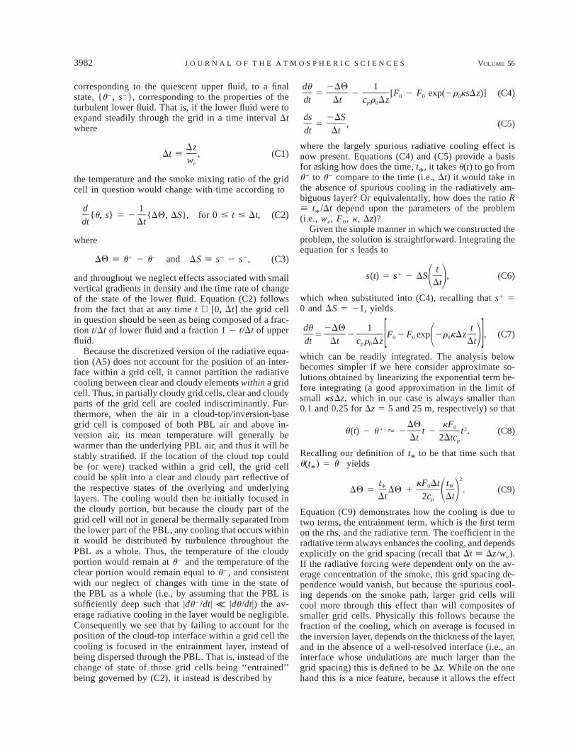
du 2DQ 15 2 [F 2 F exp(2r ksDz)] (C4)0 0 0dt Dt c r Dzp 0

ds 2DS5 , (C5)

dt Dt

where the largely spurious radiative cooling effect isnow present. Equations (C4) and (C5) provide a basisfor asking how does the time, t*, it takes u(t) to go fromu1 to u2 compare to the time (i.e., Dt) it would take inthe absence of spurious cooling in the radiatively am-biguous layer? Or equivalentally, how does the ratio R[ t*/Dt depend upon the parameters of the problem(i.e., we, F0, k, Dz)?

Given the simple manner in which we constructed theproblem, the solution is straightforward. Integrating theequation for s leads to

t1s(t) 5 s 2 DS , (C6)1 2Dt

which when substituted into (C4), recalling that s1 50 and DS 5 21, yields

du 2DQ 1 t5 2 F 2 F exp 2r kDz , (C7)0 0 01 2[ ]dt Dt c r Dz Dtp 0

which can be readily integrated. The analysis belowbecomes simpler if we here consider approximate so-lutions obtained by linearizing the exponential term be-fore integrating (a good approximation in the limit ofsmall ksDz, which in our case is always smaller than0.1 and 0.25 for Dz 5 5 and 25 m, respectively) so that

DQ kF01 2u(t) 2 u ø 2 t 2 t . (C8)Dt 2Dtcp

Recalling our definition of t* to be that time such thatu(t*) 5 u2 yields

2t* kF Dt t*0DQ 5 DQ 1 . (C9)1 2Dt 2c Dtp

Equation (C9) demonstrates how the cooling is due totwo terms, the entrainment term, which is the first termon the rhs, and the radiative term. The coefficient in theradiative term always enhances the cooling, and dependsexplicitly on the grid spacing (recall that Dt [ Dz/we).If the radiative forcing were dependent only on the av-erage concentration of the smoke, this grid spacing de-pendence would vanish, but because the spurious cool-ing depends on the smoke path, larger grid cells willcool more through this effect than will composites ofsmaller grid cells. Physically this follows because thefraction of the cooling, which on average is focused inthe inversion layer, depends on the thickness of the layer,and in the absence of a well-resolved interface (i.e., aninterface whose undulations are much larger than thegrid spacing) this is defined to be Dz. While on the onehand this is a nice feature, because it allows the effect


to vanish as Dz → 0, it also introduces an explicit res-olution sensitivity into the entrainment rate.

This explicit sensitivity is best illustrated by solving(C9) for R 5 t*/Dt:

j j jR(Dz; j) 5 2 1 1 2 , where1 2!Dz Dz Dz

c w DQp ej 5 2 , (C10)

kF0

where in the definition of j we have used (C1), that is,Dt [ Dz/we. In the special case that j/Dz → `, corre-sponding to the situation of either fine vertical resolu-tion, relatively rapid entrainment or negligible radiativeeffects (i.e., k or F0 → 0), R → 1, as one would expect.For the case of j/Dz → 0 corresponding to the limit ofcoarse vertical resolution, rapid entrainment, or rela-tively strong radiative effects, R → 0, which impliesthat all of the entrainment is spuriously driven by ra-diation.

More typical situations live between these two limits.For instance, in the case studied in this paper k 5 0.02m2 kg21, DQ ø 4 K (as taken from the mode of thedistribution in Fig. 8b with Dz 5 5 m), F0/cp ø 0.06K kg m22 s21, and we ø 0.0025 m s21 (e.g., correspond-ing to experiment 304.2 in Table 2) yields j 5 8.33.From (C10) it follows that R(25) ø 0.54 and R(5) ø0.81, thus implying an increase in entrainment rate be-tween a Dz 5 5 m calculation and a Dz 5 25 m cal-culation of 45%. Entrainment rate ratios between the 5-and 25-m calculations by the UKMO, WVU, and ARAPmodels [i.e., R(25)/R(5) 2 1] are 46% as reported byBretherton et al. (1999).8 The extent of agreement isprobably fortuitous; there is a certain amount of arbi-trariness in specifying DQ, for instance, choosing DQ5 7 K leads to a somewhat smaller prediction of R(25)/R(5) 2 1 5 33%. Moreover our use of a linearizedexponential function for the radiative flux is actually anupper bound on the effect. Because our model indicatesthat setting a threshold on the minimum smoke pathnecessary for radiation to become active can effectivelyeliminate the cooling in the radiatively ambiguous layer,it provides an explanation for the reduced sensitivity tovertical resolution in calculations that set a criticalsmoke path threshold of about s ø 0.5Dz before radi-ative fluxes become active.9 This effect is not explainedby competing ideas (e.g., Stevens and Bretherton 1999;

8 We picked these calculations because they were the only onesthat used a 5-m vertical grid in their high vertical resolution calcu-lations. The CSU and NCAR high-resolution simulations were per-formed with Dz 5 12.5 m.

9 These calculations were first presented by Hans Cuijpers, andsubsequently reproduced by us. Hans Cuijpers deserves credit fororiginally proposing what essentially amounts to this explanation.Peter Duynkerke is thanked for his tireless (and in the end contagious)advocacy of essentially these ideas.

Bretherton et al. 1999). Overall the degree of explan-atory power of the model, and its physical and quan-titative basis lead us to believe that it is the most plau-sible explanation for the sensitivity of smoke cloud sim-ulations to vertical resolution.

The simple model here has been developed for mostlyheuristic purposes. It can obviously be extended by con-sidering analogous models for simulations of waterclouds (for which case the total-water mixing ratio mustexceed the saturation threshold before liquid water isproduced and the layer becomes radiatively active), orby considering its effect given more realistic models ofwe, or by considering similar effects associated withother processes (e.g., subsidence, C. S. Bretherton andH. Grenier 1998, personal communication; Lenderinket al. 1999). A further interesting extension follows bysupposing that the buoyancy flux scales with a radia-tively based bulk Richardson number (e.g., Lock andMacVean 1999)

F0w ø A r , (C11)e 0c DQp

with A a constant of proportionality, in which case, jø A/(kr0), which says that the above-mentioned spu-rious effect scales with the ratio of the optical depth ofthe absorbing medium to the grid spacing.

Last, we emphasize that while the purely spuriouseffect discussed here may make entrainment rates ar-tificially sensitive to vertical resolution in poorly re-solved smoke cloud simulations, this should not be con-fused with in some senses a similar (albeit physical)effect associated with radiative cooling in the time-meaninterfacial layer of finite thickness evident, for instance,in simulations with well-resolved cloud-top undulations(Moeng et al. 1999).

REFERENCES

Bretherton, C. S., and Coauthors, 1999: An intercomparison of ra-diatively driven entrainment and turbulence in a smoke cloud,as simulated by different numerical models. Quart. J. Roy. Me-teor. Soc., 125, 391–423.

Clark, R. A., J. H. Ferziger, and W. C. Reynolds, 1979: Evaluationof subgrid-scale models using an accurately simulated turbulentflow. J. Fluid Mech., 91, 1–16.

Deardorff, J. W., 1980: Stratocumulus-capped mixed layers derivedfrom a three-dimensional model. Bound.-Layer Meteor., 18,495–527., G. E. Willis, and B. H. Stockton, 1980: Laboratory studies ofthe entrainment zone of a convectively mixed layer. J. FluidMech., 100, 41–64.

Ghosal, S., 1996: An analysis of numerical errors in large-eddy sim-ulations of turbulence. J. Comput. Phys., 125, 187–206.

Kraus, E. B., 1963: The diurnal precipitation change over the sea. J.Atmos. Sci., 20, 551–556.

Lenderink, G., M. C. vanZanten, and P. G. Duynkerke, 1999: Can ane–l turbulence closure simulate entrainment in convective bound-ary layers? J. Atmos. Sci., 56, 3331–3337.

Lewellen, D., and W. Lewellen, 1998: Large-eddy boundary layerentrainment. J. Atmos. Sci., 55, 2645–2665.

Lilly, D. K., 1967: The representation of small-scale turbulence innumerical simulation experiments. IBM Scientific Computing


Symp. on Environmental Sciences, Yorktown Heights, NY, IBMDP Division, 195–210., 1968: Models of cloud topped mixed layers under a stronginversion. Quart. J. Roy. Meteor. Soc., 94, 292–309.

Lock, A. P., and M. K. MacVean, 1999: A parametrization of en-trainment driven by surface heating and cloud-top cooling.Quart. J. Roy. Meteor. Soc., 125, 271–300.

Mason, P., 1989: Large eddy simulation of the convective atmosphericboundary layer. J. Atmos. Sci., 46, 1492–1516., and A. R. Brown, 1999: On subgrid models and filter operationsin large eddy simulations. J. Atmos. Sci., 56, 2101–2114.

Moeng, C.-H., 1984: A large-eddy simulation for the study of plan-etary boundary layer turbulence. J. Atmos. Sci., 41, 2052–2062., and U. Schumann, 1991: Composite structure of plumes instratus-topped boundary layers. J. Atmos. Sci., 48, 2280–2291., P. P. Sullivan, and B. Stevens, 1999: Including radiative effectsin an entrainment rate formula for buoyancy-driven PBLs. J.Atmos. Sci., 56, 1031–1049., and J. C. Wyngaard, 1989: Spectral analysis of large-eddysimulations of the convective boundary layer. J. Atmos. Sci., 45,3573–3587.

Nieuwstadt, F. T. M., P. J. Mason, C. H. Moeng, and U. Schumann,1991: Large-eddy simulation of the convective boundary layer:A comparison of four computer codes. Selected Papers Fromthe 8th Symposium on Turbulent Shear Flows, Springer-Verlag,343–367.

Patankar, S. V., 1980: Numerical Heat Transfer and Fluid Flow.Series in Computational Methods in Mechanics and ThermalSciences. McGraw Hill, 197 pp.

Pielke, R. A., and Coauthors, 1992: A comprehensive meteorologicalmodeling system—RAMS. Meteor. Atmos. Phys., 49, 69–91.

Rouse, H., and J. Dodu, 1955: Turbulent diffusion across a densitydiscontinuity. Houille Blanche, 10, 522–532.

Sayler, B. J., and R. E. Breidenthal, 1998: Laboratory simulations ofradiatively induced entrainment in stratiform clouds. J. Geophys.Res., 103, 8827–8837.

Schmidt, H., and U. Schumann, 1989: Coherent structure of the con-

vective boundary layer derived from large-eddy simulations. J.Fluid Mech., 200, 511–562.

Schumann, U., 1991: Subgrid length-scales for large-eddy simulationof stratified turbulence. Theoret. Comput. Fluid Dyn., 2, 279–290.

Sommeria, G., 1976: Three-dimensional simulation of turbulent pro-cesses in an undisturbed trade wind boundary layer. J. Atmos.Sci., 33, 216–241.

Stevens, B., W. R. Cotton, G. Feingold, and C.-H. Moeng, 1998:Large-eddy simulations of strongly precipitating, shallow, stra-tocumulus-topped boundary layers. J. Atmos. Sci., 55, 3616–3638., C.-H. Moeng, and P. P. Sullivan, 1999: Entrainment and subgridlengthscales in large-eddy simulations of atmospheric boundarylayer flows. Developments in Geophysical Turbulence, R. Kerrand Y. Kimura, Eds., Kluwer, in press.

Stevens, D., and C. S. Bretherton, 1999: Effects of resolution on thesimulation of stratocumulus entrainment. Quart. J. Roy. Meteor.Soc., 125, 425–439.

Sullivan, P. P., J. C. McWilliams, and C.-H. Moeng, 1996: A gridnesting method for large-eddy simulation of planetary boundary-layer flows. Bound.-Layer Meteor., 80, 167–202., C.-H. Moeng, B. Stevens, D. H. Lenschow, and S. D. Mayor,1998: Entrainment and structure of the inversion layer in theconvective planetary boundary layer. J. Atmos. Sci., 55, 3042–3064.

Tremback, C., J. Powell, W. R. Cotton, and R. A. Pielke, 1987: Theforward-in-time upstream advection scheme: Extension to higherorders. Mon. Wea. Rev., 115, 3540–555.

Turner, J. S., 1986: Turbulent entrainment: The development of theentrainment assumption, and its application to geophysical flows.J. Fluid Mech., 173, 431–471.

vanZanten, M. C., P. G. Duynkerke, and J. W. M. Cuijpers, 1999:Entrainment parameterization in convective boundary layers de-rived from large eddy simulations. J. Atmos. Sci., 56, 813–828.

Zalesak, S. T., 1979: Fully multidimensional flux-corrected transportalgorithms for fluids. J. Comput. Phys., 31, 335–362.

large-eddy simulations of radiatively driven …€¦ · large-eddy simulations of radiatively...

Documents