large eddy simulations: how to evaluate...
TRANSCRIPT
Large Eddy Simulations: how to evaluate resolution
Lars Davidson
Division of Fluid Dynamics, Department of Applied Mechanics, Chalmers University of
Technology, SE-412 96 Goteborg, Sweden
Abstract
Int. J. of Heat and Fluid Flow, Vol. 30(5), pp. 1016-1025, 2009
The present paper gives an analysis of fully developed channel flow at Reynolds
number of Re = uτδ/ν = 4000 based on the friction velocity, uτ , and half
the channel height, δ. Since the Reynolds number is high, the LES is cou-
pled to a URANS model near the wall (hybrid LES-RANS) which acts as
a wall model. It it found that the energy spectra is not a good measure of
LES resolution; neither is the ratio of the resolved turbulent kinetic energy
to the total one (i.e. resolved plus modelled turbulent kinetic energy). It is
suggested that two-point correlations are the best measures for estimating
LES resolution. It is commonly assumed that SGS dissipation takes place at
high wavenumbers. Energy spectra of the fluctuating velocity gradients show
that this is not true; the major part of the SGS dissipation takes place at
low to midrange wavenumbers. Furthermore, the energy spectra of the fluc-
tuating velocity gradients reveals that the accuracy of the predicted velocity
Email address: [email protected] (Lars Davidson)URL: www.tfd.chalmers.se/~~11~lada (Lars Davidson)
Preprint submitted to International Journal of Heat and Fluid Flow June 17, 2009

gradients at the highest resolved wavenumbers is very poor.
Key words: LES, two-point correlations, energy spectra, dissipation
spectra, SGS dissipation
1. Introduction
In wall-bounded Direct Numerical Simulations (DNS) and Large Eddy
Simulations (LES) numerical experiments were carried out to determine the
minimum required resolution to obtain accurate results (Moin and Kim, 1982;
Piomelli, 1993; Piomelli and Chasnov, 1996; Moser et al., 1999; Hoyas and
Jimenez, 2006). The grid resolution in DNS and wall-resolved LES is dictated
by the necessity of resolving the energy-generating process high-speed in-
rushes and low-speed ejections (Robinson, 1991) in the viscous sub-layer and
the buffer layer, often called the streak process. Since this process takes place
in the viscous-dominating near-wall region, the required grid resolution must
be expressed in inner variables, i.e. viscous units. In LES, the required grid
resolution is ∆x+ ≃ 100, y+ ≃ 1 (wall-adjacent cell centers) and ∆z+ ≃ 30
where x, y, z denote the streamwise, wall-normal and spanwise directions,
respectively. Since a viscous length unit compared to the boundary layer
thickness becomes smaller the higher the Reynolds number, the simulation
times for DNS and wall-resolved LES at high Reynolds numbers become
prohibitively high.
In the past ten years much research has been dedicated to the task of find-
2
ing wall models that circumvent the requirement of defining the minimum
near-wall cell size using inner variables. Spalart and his co-worker first pro-
posed Detached-Eddy Simulations (Spalart et al., 1997; Travin et al., 2000),
abbreviated as DES; later, different variants of hybrid LES/RANS models
were proposed (Davidson and Peng, 2003; Temmerman et al., 2002; Tucker
and Davidson, 2004; Hamba, 2003). In both DES and hybrid LES/RANS, the
region near the walls is treated with Unsteady Reynolds-Averaged Navier-
Stokes (URANS) and the outer region is treated by LES; the main difference
is that, in DES, the entire boundary layer is treated with URANS whereas,
in hybrid LES/RANS, the interface between URANS and LES is located in
the inner part of the logarithmic region.
Another way to model the near-wall region is to use two-layer mod-
els (Balaras et al., 1996; Cabot, 1995; Cabot and Moin, 1999; Wang and
Moin, 2002), also called “thin boundary layer equations”. Here, the first
node in the LES simulations is located – as when using wall functions – in
the log-region. A new fine near-wall mesh is then created covering the wall-
adjacent LES cell. Good results have been obtained for flow around a smooth
three-dimensional hill (Tessicini et al., 2007), which is a fairly complex flow.
Even wall functions — based on the instantaneous log-law — were found to
give good results for this flow (Tessicini et al., 2007).
Assuming that the near-wall region is modelled using, for example, one
3

of the approaches mentioned above, the question arises: how fine does the
mesh need to be in the LES region? And, how do we, after having made an
LES (assuming that there are no experimental data with which to compare),
verify that the resolution was good enough? This is the focus of the present
paper.
There are different ways to estimate the resolution of LES data. The
first measure is probably to compare the modelled turbulence and stresses
with the resolved ones. The smaller the ratio, the better the resolution.
Another, similar way, is to compare the resolved turbulent kinetic energy
to the modelled one. The energy spectra are commonly computed to find
out whether they exhibit a −5/3 range and if they do the flow is considered
to be well resolved. Another measure of the resolution may be to look at
the two-point correlations to identify, for example, the ratio of the integral
length scale to the cell size. A less common approach is to compare the
SGS (i.e. modelled) dissipation due to fluctuating resolved strain-rates to
that due to resolved or time-averaged strain-rates. In steady RANS, all SGS
dissipation takes place due to time-averaged strain-rates whereas, in a well-
resolved LES, most of the SGS dissipation occurs due to resolved fluctuations.
It is commonly assumed that the SGS dissipation takes place at the highest
resolved wavenumbers. This can be verified or disproved by making energy
spectra of the SGS dissipation to find the wavenumbers at which the SGS
4
dissipation does in fact take place.
The approaches mentioned above are used in the present paper to evaluate
how relevant they are in estimating the resolution of LES simulations of fully
developed channel flow. The Reynolds number is 4000 based on the friction
velocity and the half-height of the channel. Five different resolutions are
used. In order to be able to carry out LES at high Reynolds number, the
near-wall region is covered by a wall model. In this work we have chosen to
use hybrid LES/RANS.
The paper is organized as follows. The first three sub-sections present
the equations, the turbulence model and the numerical method. The fol-
lowing section presents and analyzes the results using different resolutions.
Conclusions are given in the final section.
2. Numerical details
2.1. The Momentum Equations
The Navier-Stokes equations with an added turbulent/SGS viscosity read
∂ui
∂t+
∂
∂xj(uiuj) = δ1i −
1
ρ
∂p
∂xi+
∂
∂xj
[
(ν + νT )∂ui
∂xj
]
∂ui
∂xi
= 0
(1)
where νT = νt (νt denotes the turbulent RANS viscosity) close to the wall
for y ≤ yml, otherwise νT = νSGS. The location at which the switch is made
from URANS to LES is called the interface and is located at yml from each
5

y
x
wall
wall
URANS region
URANS region
LES region
y+
ml
jml
Figure 1: The LES and URANS regions. The interface is located at y+ = y+
ml and the
number of cells in the URANS region in the wall-normal direction is jml.
wall, see Fig. 1. The turbulent viscosity, νT , is computed from an algebraic
turbulent length scale, see Table 1, and a transport equation is solved for kT ,
see below. The density is set to one in all simulations. A driving constant
pressure gradient, δ1i, is included in the streamwise momentum equation.
2.2. Hybrid LES–RANS
A one-equation model is employed in both the URANS region and the
LES region and reads
∂kT
∂t+
∂
∂xj
(ujkT ) =∂
∂xj
[
(ν + νT )∂kT
∂xj
]
+ PkT− Cε
k3/2
T
ℓ
PkT= −τij sij , τij = −2νT sij
6

where νT = ck1/2ℓ. In the inner region (y ≤ yml) kT corresponds to RANS
turbulent kinetic energy, k; in the outer region (y > yml) it corresponds to
subgrid-scale kinetic turbulent energy, kSGS. The coefficients are different in
the two regions, see Table 1. No special treatment is applied in the equations
at the matching plane except that the form of the turbulent viscosity and
the turbulent length scale are different in the two regions.
2.3. The Numerical Method
An incompressible, finite volume code is used (Davidson and Peng, 2003).
For space discretization, central differencing is used for all terms except the
convection term in the kT equation, for which the hybrid central/upwind
scheme is employed. The Crank-Nicolson scheme is used for time discretiza-
tion of all equations. The numerical procedure is based on an implicit, frac-
tional step technique with a multigrid pressure Poisson solver (Emvin, 1997)
URANS region LES region
ℓ κc−3/4µ n[1 − exp(−0.2k1/2n/ν)] ℓ = ∆
νT κc1/4µ k1/2n[1 − exp(−0.014k1/2n/ν)] 0.07k1/2ℓ
Cε 1.0 1.05
Table 1: Turbulent viscosities and turbulent length scales in the URANS and LES regions.
n denotes the distance to the nearest wall. ∆ = (δV )1/3
.
7
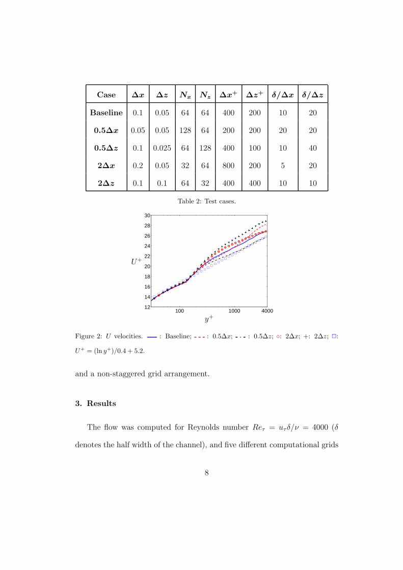
Case ∆x ∆z Nx Nz ∆x+∆z+ δ/∆x δ/∆z
Baseline 0.1 0.05 64 64 400 200 10 20
0.5∆x 0.05 0.05 128 64 200 200 20 20
0.5∆z 0.1 0.025 64 128 400 100 10 40
2∆x 0.2 0.05 32 64 800 200 5 20
2∆z 0.1 0.1 64 32 400 400 10 10
Table 2: Test cases.
100 1000 400012
14
16
18
20
22
24
26
28
30
y+
U+
Figure 2: U velocities. : Baseline; : 0.5∆x; : 0.5∆z; ◦: 2∆x; +: 2∆z; 2:
U+ = (ln y+)/0.4 + 5.2.
and a non-staggered grid arrangement.
3. Results
The flow was computed for Reynolds number Reτ = uτδ/ν = 4000 (δ
denotes the half width of the channel), and five different computational grids
8

0 1000 2000 3000 4000−1
−0.8
−0.6
−0.4
−0.2
0
〈u′ v
′ 〉
y+
Figure 3: Resolved shear stress. For legend, see caption in Fig. 2.
are used, see Table 2. The number of cells in the y direction is 80 with a
constant geometric stretching of 15%. This gives a smallest and largest cell
height of ∆y+
min = 2.2 and ∆y+max = 520, respectively. The grid spacing in the
wall-parallel plane in viscous units is (∆x+, ∆z+)=(200–800, 100–400). The
extent of the domain in the x and z directions is 6.4 and 3.2, respectively,
for all cases. The matching line is chosen along a fixed grid line at y+ = 125
(y = 0.0313) so that 16 cells are located in the URANS region at each
wall. It should be mentioned that in the present work the matching line
between the URANS and the LES regions is located rather close to the
wall. If the matching line were located as in DES (i.e. min(0.65∆m, y),
∆m = max(∆x, ∆y, ∆z)), the agreement would have been much better for
all five cases. However, the object of this work was not to obtain the best
possible results, but to compared different ways of estimating the resolution.
9
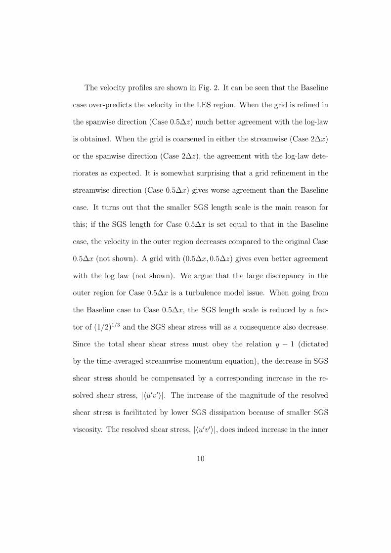
The velocity profiles are shown in Fig. 2. It can be seen that the Baseline
case over-predicts the velocity in the LES region. When the grid is refined in
the spanwise direction (Case 0.5∆z) much better agreement with the log-law
is obtained. When the grid is coarsened in either the streamwise (Case 2∆x)
or the spanwise direction (Case 2∆z), the agreement with the log-law dete-
riorates as expected. It is somewhat surprising that a grid refinement in the
streamwise direction (Case 0.5∆x) gives worse agreement than the Baseline
case. It turns out that the smaller SGS length scale is the main reason for
this; if the SGS length for Case 0.5∆x is set equal to that in the Baseline
case, the velocity in the outer region decreases compared to the original Case
0.5∆x (not shown). A grid with (0.5∆x, 0.5∆z) gives even better agreement
with the log law (not shown). We argue that the large discrepancy in the
outer region for Case 0.5∆x is a turbulence model issue. When going from
the Baseline case to Case 0.5∆x, the SGS length scale is reduced by a fac-
tor of (1/2)1/3 and the SGS shear stress will as a consequence also decrease.
Since the total shear shear stress must obey the relation y − 1 (dictated
by the time-averaged streamwise momentum equation), the decrease in SGS
shear stress should be compensated by a corresponding increase in the re-
solved shear stress, |〈u′v′〉|. The increase of the magnitude of the resolved
shear stress is facilitated by lower SGS dissipation because of smaller SGS
viscosity. The resolved shear stress, |〈u′v′〉|, does indeed increase in the inner
10

region when going from the Baseline case to Case 0.5∆x, see Fig. 3. How-
ever, in the outer region – in which the velocity gradient is much smaller –
the flow is initially not able to increase the magnitude of the resolved shear
stress. Hence, in order to satisfy the linear law of the total shear, the magni-
tude of the SGS shear stress must increase and the flow accomplishes this by
increasing the velocity gradient for y+ > 1000, see Fig. 2. Careful inspection
of Fig. 3 reveals that also the magnitude of the resolved shear stress for Case
0.5∆x is slightly larger (for 1500 < y+ < 3000) than for the Baseline case.
The question then arises why the agreement of the velocity profile with the
log law does not deteriorate when the grid is refined in the spanwise direction
(Case 0.5∆z). The answer is that the refinement in the spanwise direction
allows additional turbulence to be resolved (the peak of |〈u′v′〉| is larger for
Case 0.5∆z than for Case 0.5∆x) which compensates for the decrease in the
SGS shear stress. The discussion above indicates that it could be interesting
to develop new SGS models in which the SGS length scale is sensitized to the
magnitude of the resolved strain, (2sij sij)1/2; if the resolved strain is large,
the length scale can be taken as ∆, but if it is small the length scale should
maybe be larger.
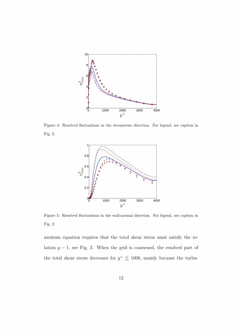
Figures 4 and 5 present the streamwise and wall-normal resolved fluctu-
ations, respectively. As can be seen, u2rms and v2
rms increases and decreases,
respectively, as the grid is coarsened. The time-averaged streamwise mo-
11
0 1000 2000 3000 40000
2
4
6
8
10
u2 rm
s
y+
Figure 4: Resolved fluctuations in the streamwise direction. For legend, see caption in
Fig. 2.
0 1000 2000 3000 40000
0.2
0.4
0.6
0.8
1
v2 rm
s
y+
Figure 5: Resolved fluctuations in the wall-normal direction. For legend, see caption in
Fig. 2.
mentum equation requires that the total shear stress must satisfy the re-
lation y − 1, see Fig. 3. When the grid is coarsened, the resolved part of
the total shear stress decreases for y+ . 1000, mainly because the turbu-
12

0 1000 2000 3000 40000
5
10
15
20
25
30
35
40
〈νT〉/
ν
y+
Figure 6: Turbulent viscosity. For legend, see caption in Fig. 2.
0 200 400 600 800 1000
−0.55
−0.5
−0.45
−0.4
Cuv
y+
Figure 7: The correlation coefficient, Cuv = 〈u′v′〉/(urmsvrms). For legend, see caption in
Fig. 2.
lent viscosity increases with grid coarsening, see Fig. 6. Furthermore, the
non-linear interaction is weakened so that, in the region of maximum |〈u′v′〉|
(i.e. 200 < y+ < 600), the correlation between the streamwise and wall-
normal resolved fluctuations is diminished, see Fig. 7 (this is also seen in
coarse DNS (Davidson and Billson, 2006)). Initially, this results in too small
13

0 1000 2000 3000 40000
0.5
1
1.5
2
w2 rm
s
y+
Figure 8: Resolved fluctuations in the spanwise direction. For legend, see caption in Fig. 2.
a) 0 1000 2000 3000 4000
−2
0
2
4
6
−2〈
v′ ∂
p′/∂
y〉
y+ b) 0 1000 2000 3000 40000
5
10
15
20
25
−2〈
w′ ∂
p′/∂
z〉
y+
Figure 9: Pressure-gradient-velocity terms in the (a) v2rms and (b) w2
rms equations. For
legend, see caption in Fig. 2.
a resolved shear stress. The equations respond by increasing the resolved
fluctuations by increasing the bulk velocity and hence the velocity gradient,
∂u/∂y, which is the main agent for producing resolved turbulence. The bulk
velocity, and hence the resolved fluctuations, are increased until the resolved
shear stress is large enough so that the total shear stress satisfies the linear
14

a) 0 1000 2000 3000 40000
1
2
3
4
5
6
kres
y+ b) 0 1000 2000 3000 40000.4
0.5
0.6
0.7
0.8
0.9
1
γ
y+
Figure 10: Resolved turbulent kinetic energy kinetic energy and the ratio γ (Eq. 2). For
legend, see caption in Fig. 2.
relation. Because of the damping effect of the wall on v′, the equations in-
crease u′ until the linear relation is obtained. This explains the large values
of u2rms in Fig. 4 for the coarse resolutions. It should be stressed that the pro-
cess of increasing the resolved fluctuations until the total shear stress satisfies
the linear relation y − 1 does not occur in a general flow case with an inlet
and outlet (i.e. a flow case with no prescribed driving pressure gradient). In
a general flow case, the magnitude of the resolved shear stresses will simply
remain too small.
The spanwise fluctuations increase when the grid is coarsened in the span-
wise direction, whereas they decrease upon coarsening in the streamwise di-
rection, see Fig. 8. They increase when the grid is refined. Furthermore,
the location of the peak is not affected neither by grid coarsening nor grid
refinement. This behaviour is completely different from that of the wall-
15

normal stresses. The different behavior of the wall-normal fluctuations and
the spanwise fluctuations is explained by Fig. 9, where the pressure-gradient-
velocity terms are presented; these terms are the main source terms in the
transport equations of v2rms and w2
rms. It can be seen that the term in the
v2rms equation — like v2
rms itself — decreases/increases in the LES region for
y+ < 1000 when the grid is coarsened/refined and that the peak of the source
term moves away from the wall. The term in the w2rms equation, however,
shows a different behavior when the grid is coarsened in the spanwise or the
streamwise direction: it increases in the former case whereas it increases in
the latter case. When the grid is refined in the streamwise direction, the
source term increases. This agrees with the behavior of w2rms, see Fig. 8. A
conclusion from the discussion above is that it is crucial to properly resolve
the interaction between fluctuating resolved velocities and pressure.
The resolved turbulent kinetic energy is presented in Fig. 10a, and since
it is dominated by the streamwise fluctuations, its behavior is similar to that
of u2rms. Pope (2004) suggests that when 80% of the turbulent kinetic energy
is resolved, i.e.
γ =kres
< kT > +kres> 0.8, kres =
1
2〈u′
iu′i〉, (2)
the LES can be consider to be well-resolved. Figure 10b presents this ratio
and as can be seen it is, in the LES region, larger than 85% for all grids.
Hence this quantity does not seem to be a good measure of the resolution.
16

0 0.5 1 1.5 20
0.2
0.4
0.6
0.8
1
x
Buu(x
)/u
2 rm
s
Figure 11: Normalized two-point correlation Buu(x)/u2rms. y = 0.11. For legend, see
caption in Fig. 2. Markers on the lines show the resolution.
0 0.2 0.4 0.6 0.8−0.2
0
0.2
0.4
0.6
0.8
1
x
Bw
w(x
)/w
2 rm
s
Figure 12: Normalized two-point correlation Bww(x)/w2rms. y = 0.11. For legend, see
caption in Fig. 2. Markers on the lines show the resolution.
Figures 11, 12 and 13 present the streamwise and spanwise two-point
correlations, which are defined as Buu(x) = 〈u′(x)u′(x − x)〉, Bww(x) =
〈w′(x)w′(x− x)〉 and Bww(z) = 〈w′(z)w′(z− z)〉, respectively. The two-point
17

0 0.1 0.2 0.3 0.4−0.2
0
0.2
0.4
0.6
0.8
1
Bw
w(z
)/w
2 rm
s
z
Figure 13: Normalized two-point correlation Bww(z)/w2rms. y = 0.11. Markers on the
lines show the resolution. For legend, see caption in Fig. 2.
correlations are all presented for y+ ≃ 440 (y = 0.11); they do not vary much
across the channel. The two-point correlations are normalized with u2rms and
w2rms, respectively. In Fig. 11, 12, the two-point correlations increase when
the grid is coarsened (Cases 2∆x and 2∆z) because the smaller scales are
not resolved; for these coarse resolutions the streamwise two-point correla-
tions are dominated by the “superstreaks” (Piomelli et al., 2003; Keating
and Piomelli, 2006). When the grid is refined (Cases 0.5∆x and 0.5∆z), the
two-point correlations decrease, as expected. For Case 2∆x, the two-point
correlation formed with u′ (Fig. 11) falls down to 0.4 within four cells. In
the spanwise direction it is even worse: for Case 2∆z the two-point corre-
lation goes to zero within two cells (Fig. 13). The reason is that the grid
is so coarse that the non-linear process of generating turbulence cannot be
18

100
101
10−8
10−6
10−4
10−2
Ew
w(k
x)
κx = 2π(kx − 1)/xmax
Figure 14: Energy spectra Eww(kx). y = 0.11. The thick dashed line shows −1 slope. For
legend, see caption in Fig. 2.
100
101
10−6
10−4
10−2
100
101
Euu(k
x)
κx = 2π(kx − 1)/xmax
Figure 15: Energy spectra Euu(kx). y = 0.11. The thick dashed line shows −1 slope. For
legend, see caption in Fig. 2.
sustained. This is a clear indication that the resolution is too poor for Cases
2∆x and 2∆z.
Figures 14 and 15 present the one-dimensional energy spectra Eww(kx)
19

100
101
102
10−4
10−3
10−2
10−1
Ew
w(k
z)
κz = 2π(kz − 1)/zmax
Figure 16: Energy spectra Eww(kz). y = 0.11. The thick dashed line shows −5/3 slope.
For legend, see caption in Fig. 2.
and Euu(kx). The smallest wavenumber is κx,min = 2π/xmax = 2π/6.4 =
0.98. The largest wavenumber included in the plot is κx,max = 2π/2∆x,
where we have assumed that two cells are required to resolve a wavelength.
For the Baseline case, for example, this gives κx,max = π/0.1 = 31. The
energy spectrum Eww(kx) = W 2, for example, is computed by the DFT
(Discrete Fourier Transform) of w′
W (kx) =1
Nx
Nx∑
n=1
w′(n)
[
cos
(
2π(n − 1)(kx − 1)
Nx
)
−ı sin
(
2π(n − 1)(kx − 1)
Nx
)]
(3)
where W are the complex Fourier coefficients of w′ and ı2 = −1; the normal-
ized streamwise coordinate appears at the right side as (n−1)/Nx = x/xmax.
The w2rms can be retrieved by summing the square of the real and imaginary
20
parts of W , i.e.
w2
rms =
Nx∑
n=1
(Re(W (kx)))2 + (Im(W (kx)))
2 (4)
The energy spectra are all presented for y+ ≃ 440 (y = 0.11) but, when
plotted in log-log as in Figs. 14 and 15, they show the same behavior across
the channel, the main difference being that they are shifted along the Eww
Euu axes as w2rms and u2
rms vary across the channel. For comparison, a slope
of “−1” is included in the figures. For high wavenumbers (kx > 7 for Eww
and kx > 10 for Euu), the streamwise energy spectra for the Case 2∆x
exhibits a clear “dissipation” range (i.e. a steeper slope than −5/3). For the
other cases the dissipation range starts at higher wavenumbers. If the energy
spectra had been obtained from DNS or experiments, it would indeed have
been a dissipation range but, in the present case, we are using a turbulence
model and hence what is seen in the energy spectra is an SGS dissipation
range.
Figure 16 shows the spanwise energy spectra of the spanwise fluctuations.
A line with a −5/3 slope is included for comparison. As can be seen, no −5/3
range exists. The energy spectra for all cases show a tendency of pile-up of
energy in the small scales. This phenomenon is present across the channel.
The spanwise energy spectra presented, Fig. 16, do not actually give much
guidance as to whether the resolution is sufficient. With an effort, one could
find a −5/3 range for the Baseline case, Cases 0.5∆x and 0.5∆z, indicating
21

a)0 10 20 30 40 50 60
0
0.5
1
1.5
2
2.5x 10
−3
2ν·P
SD
(∂w
′ /∂x)
κx = 2π(kx − 1)/xmaxb)
0 10 20 30 40 50 600
0.5
1
1.5
2
2.5
3
3.5
4x 10
−3
2νk
2 xE
ww(k
x)
κx = 2π(kx − 1)/xmax
Figure 17: Energy spectra of an exact and approximated spanwise component of viscous
dissipation versus streamwise wavenumber. y = 0.11. For legend, see caption in Fig. 2.
that these resolutions all are sufficient. But from the two-point correlations
in Fig. 13 we find that the largest scales are covered by 4, 4 and 8 cells,
respectively. Only Case 0.5∆z could be considered to be sufficient. The
streamwise energy spectra, Figs. 14 and 15, indicate that the resolution is
too coarse for all cases (no −5/3 range). The two-point correlation for Case
0.5∆x (Fig. 11), for example, shows that the largest scales are covered by
some 16 cells which should be sufficient.
The energy spectra in Fig. 16 indicate that SGS dissipation is active
at relatively low wave numbers (the pile-up of energy at high wavenumbers
shows that the SGS dissipation is small at high wavenumbers). To investigate
this further, we will study the spectra of the dissipation. The two-point
correlation, Bww(z), is the inverse DFT of the symmetric energy spectrum,
22

a)0 20 40 60 80 100 120
0
0.5
1
1.5
2
2.5
3
3.5
4x 10
−3
2ν·P
SD
(∂w
′ /∂z)
κz = 2π(kz − 1)/zmaxb)
0 20 40 60 80 100 1200
0.005
0.01
0.015
2νk
2 zE
ww(k
z)
κz = 2π(kz − 1)/zmax
Figure 18: Energy spectra of an exact and approximated spanwise component of viscous
dissipation versus spanwise wavenumber. y = 0.11. For legend, see caption in Fig. 2.
0 1000 2000 3000 40000
0.1
0.2
0.3
0.4
0.5
0.6
0.7
0.8
y+
ε′ SG
S,x
+z/ε
′ SG
S
Figure 19: Ratio of SGS dissipation due to resolved fluctuations in the wall-parallel plane
to the total one, see Eq. 9. For legend, see caption in Fig. 2.
Eww, i.e.
Bww(z/zmax) =
Nz∑
kz=1
Eww(kz) cos
(
2π(kz − 1)(n − 1)
Nz
)
where Nz is the number of cells in the spanwise direction; the normalized
23

K kres
⟨
u′iu
′j
⟩ ∂〈ui〉
dxj
〈kT 〉
〈νT〉∂〈u
i〉
∂xj
∂〈ui〉
∂xj
EI
ν ∂〈ui 〉∂x
j
∂〈ui 〉∂x
j
ε
ν
⟨ ∂u′i
∂xj
∂u′i
∂xj
⟩
ε ′SGS
Figure 20: Transfer of kinetic turbulent energy between time-averaged, resolved, modelled
kinetic energy and internal energy. K = 1
2〈ui〉〈ui〉 and kres = 1
2〈u′
iu′
i〉 denote time-
averaged kinetic and resolved turbulent kinetic energy, respectively. EI denotes internal
energy. ε is viscous dissipation at subgrid scales, see Eq. 10.
0 200 400 600 800 10000
0.2
0.4
0.6
0.8
1
ε′ SG
S/ε
SG
S
y+
0 200 400 600 800 10000
5
10
15
20
25
30
35
40
ε′ SG
S
y+
Figure 21: SGS dissipation due to resolved fluctuations, ε′SGS , see Eq. 9. For legend, see
caption in Fig. 2.
24

spanwise separation distance appears at the right side as (n−1)/Nz = z/zmax.
εwz can — in theory — be obtained from (Hinze, 1975)
εwz = 2ν
⟨
(
∂w′
∂z
)2⟩
= 2ν∂2Bww(z)
∂z2
∣
∣
∣
∣
z=0
= 2ν
Nz∑
kz=1
κ2
zEww(kz) (5)
where κz = 2π(kz − 1)/zmax. However, this relation is not satisfied at the
discrete level, because the derivative ∂w′/∂z cannot be evaluated exactly in
a finite-volume approach (the relation would have been satisfied had we used
a spectral method solving for the Fourier coefficients), and thus
εwz,FV 6= 2ν
Nz∑
kz=1
κ2
zEww,FV (kz) (6)
where subscript FV denotes Finite Volume. Instead, a DFT of ∂w′/∂z as
Dz(kz) =1
Nz
Nz∑
n=1
∂w′(n)
∂z
[
cos
(
2π(n − 1)(kz − 1)
Nz
)
−ı sin
(
2π(n − 1)(kz − 1)
Nz
)]
(7)
must be formed where Dz are the complex Fourier coefficients of ∂w′/∂z.
Then the Power Spectral Density, i.e. Dz ∗ D∗z , where superscript ∗ denotes
complex conjugate, can be formed. Now indeed (cf. Eq. 4)
εwz,FV = εwz,exact = 2νNz∑
kz=1
Dz ∗ D∗z = 2ν
Nz∑
kz=1
PSD(∂w′/∂z). (8)
Figures 17 and 18 present the energy spectra of the resolved velocity gradi-
ents ∂w′/∂x and ∂w′/∂z. As mentioned above, κ2xEww(kx) and PSD(∂w′/∂x),
and κ2zEww(kz) and PSD(∂w′/∂z), respectively, should in theory be equal;
25

as can be seen, the former are larger than the latter. The discrepancy is in
effect a measure of the inaccuracy of the finite volume method in estimating
a derivative, and the error becomes larger for small spanwise scales (large
spanwise wavenumbers, κz). Although Eq. 5 is formally exact, the correct
way to create a spectrum of the computed results is to use Eqs. 7 and 8. The
reason is that, in Eqs. 7 and 8, the velocity gradients are estimated in the
same way as when predicting the flow, whereas the velocity gradients in Eq. 5
are estimated with higher accuracy (actually exactly) than when predicting
the flow. Furthermore, the predicted dissipation in the physical and spectral
space agrees when Eq. 7 is used, whereas they do not when Eq. 5 is used.
It is commonly assumed that the major part of the SGS dissipation takes
place close to the cut-off, i.e. at high resolved wavenumbers. Figures 17a and
18a show that this is not the case at all. The peaks of the resolved velocity
gradients are located at kx, kz < 20. This explains the strong decay in the
energy spectra in Figs. 14, 15 and 16. For wavenumbers, kx, larger than
20, no dissipation takes place for any resolution except for Case 0.5∆x, see
Fig. 17a.
The dissipation energy spectra in the spanwise direction show a large
discrepancy at high wavenumbers between the exact ones (Eqs. 7, 8, Fig. 18a)
and those computed from the energy spectra of w′ (Eq. 5, Fig. 18b). This is
an indication of how poorly the velocity gradients are resolved for the higher
26

wavenumbers.
When the dissipation spectra presented above are plotted in the center
of the channel, they do not change a great deal except that the peaks are
shifted slightly towards lower wavenumbers.
Above, components of the energy spectra for the viscous dissipation (e.g.
ν(∂w′/∂z)2) rather than for the SGS dissipation (e.g. νT (∂w′/∂z)2) are pre-
sented. The main reason for this is that it is only for the viscous dissipation
that Eq. 5, in theory, holds. Actually, the exact spectrum of νT (∂w′/∂z)2
has been computed (note that in this case the Fourier coefficients in Eq. 7
are formed with ν0.5T ∂w′/∂z, whose physical meaning is somewhat obscure),
and it is found that the two energy spectra are very similar; one difference
is that, unlike for the viscous dissipation, the first Fourier mode is non-zero
for the SGS dissipation because 〈ν0.5T ∂w′/∂z〉 6= 0 whereas 〈ν∂w′/∂z〉 = 0.
Above we have only analyzed the dissipation spectra due to spanwise
and streamwise derivatives. One reason is that the spanwise and streamwise
components of the SGS dissipation make an important contribution to the
total one. Figure 19 shows the ratio of the SGS dissipation in the wall-parallel
plane, ε′SGS,x+z, to the total SGS dissipation, ε′SGS, where
ε′SGS = εSGS − ε〈SGS〉 =
⟨
νT∂ui
∂xj
∂ui
∂xj
⟩
− 〈νT 〉
(
∂〈u〉
∂y
)2
ε′SGS,x+z =
⟨
νT∂ui
∂x1
∂ui
∂x1
+ νT∂ui
∂x3
∂ui
∂x3
⟩(9)
The contribution of ε′SGS,x+z to ε′SGS is close to 35% or larger for all cases
27

except Case 2∆z, see Fig. 19. Another reason why we have not included the
wall-normal derivative in the analyze in Figs. 17 and 18 is that Eq. 5 does
not hold for this derivative (x2 is not an homogeneous direction).
Figure 20 presents the flow of kinetic energy between the time-averaged
kinetic energy, 〈ui〉〈ui〉/2, the resolved fluctuating kinetic energy, 〈u′iu
′i〉/2,
the modelled (SGS) kinetic energy, 〈kT 〉, and the energy flow of all three
kinetic energies down to the internal energy, EI , i.e. viscous dissipation. ε
denotes viscous dissipation at the subgrid scales, i.e.
ε = ν
⟨
∂u′i,SGS
∂xj
∂u′i,SGS
∂xj
⟩
, kSGS =1
2〈u′
i,SGSu′i,SGS〉 (10)
In steady RANS using an eddy-viscosity model the right circle vanishes, and
most of the energy flow goes from K to kT and only a small fraction directly
from K to EI (assuming low Mach number flow). In a well-resolved LES, the
energy transfers from K to kT and the transfer from K to EI is negligible.
In this case, the flow of kinetic energy goes from K to kres, and from kres to
kT , and then to EI . Only a small fraction goes from kres to EI .
From the discussion above in relation to Fig. 20, it is clear that an in-
dicator of how well the flow is resolved is a comparison of the modelled
dissipation from K and kres. The modelled dissipation in the kres equation
is taken as ε′SGS, see Eq. 9. Figure 21 presents εSGS and ε′SGS. As expected,
the SGS dissipation due to the time-averaged flow dominates in the URANS
region (y+ < 125) near the wall, see Fig. 21a. Further away from the wall
28
(160 ≤ y+ ≤ 200, depending on the resolution), the ε′SGS/εSGS ratio becomes
larger than one half and is, for y+ > 800, larger than 0.9 for all cases. It can
also be seen in Fig. 21a that, the higher resolution, the higher the ε′SGS/εSGS
ratio; however, when ε′SGS is not normalized with εSGS (Fig. 21b), the picture
is reversed, i.e. coarse resolution gives large ε′SGS. The results in Fig. 21b
are partly explained by the high turbulent viscosity for the coarse resolutions
(Fig. 6) and partly by higher turbulent resolved fluctuations. The correct ap-
proach is to present ε′SGS in normalized form (Fig. 21a) because, in this way,
the influence of the background flow is minimized; the ε′SGS presented in
Fig. 21b are biased by different mean flows, resolved turbulent fluctuations
and SGS viscosities.
4. Conclusions
Five different grid resolutions have been investigated: Baseline (∆x, ∆z),
two cases with a refined grid (0.5∆x and 0.5∆z) and two cases with a coars-
ened grid (2∆z and 2∆z). The resolution in the streamwise direction lies
in the interval 200 ≤ x+ ≤ 800 and 5 ≤ δ/∆x ≤ 20 and in the spanwise
direction 100 ≤ z+ ≤ 400 and 10 ≤ δ/∆z ≤ 40.
From the two-point correlations we find by how many cells the largest
scales are resolved. This is very useful information. It is up to the re-
searcher/engineer to decide how many cells he/she deems necessary, but the
29

recommended minimum for a coarse LES should be at least four cells, prefer-
ably more than double that. Note that also eight cells is usually very far from
a well-resolved LES. The two-point correlations presented in this work reveal
that the resolutions for Cases 2∆x and 2∆z are much too coarse. Case 2∆z
yields almost zero two-point correlation at a separation distance of two cells.
It is suggested that two-point correlations in the poorest resolved direction
(the spanwise direction in the present work) are suitable for estimating the
resolution.
Pope (2004) suggests that if the ratio of the resolved turbulent kinetic
energy to the total (i.e. the resolved plus the modelled) is larger than 80%,
the LES simulation is well-resolved. The present work indicates that this is
not a good measure because, for all five cases, this ratio is larger than 85%.
One-dimensional energy spectra obtained from the two-point correlations
have been presented. It is concluded that they are not useful for estimating
the resolution.
It is found that the resolved streamwise fluctuation and the resolved tur-
bulent kinetic energy increase, and that the correlation coefficient, 〈−u′v′〉/(urmsvrms),
decreases as the grid is coarsened. These phenomena are coupled to each
other, since the time-averaged flow must satisfy a linear variation of the to-
tal shear stress. The correlation between u′ and v′ is weakened when the
grid is coarsened, and the equations compensate for this by increasing the
30

product of urms and vrms.
The spanwise resolved fluctuation, wrms, and the wall-normal one behave
differently when the grid is refined and coarsened. Their behavior is explained
by their largest source terms, the pressure velocity terms, −2〈w′∂p′/∂z〉
(w2rms equation) and −2〈v′∂p′/∂y〉 (v2
rms equation). Hence, it is seems that
it is vital to accurately capture the interaction of the fluctuating velocities
and pressure. Possibly some work should be directed towards development
of discretization schemes which accurately treat the pressure-velocity cou-
pling. Presumably, iterative solvers which treat pressure and velocities in a
segregated manner (such as pressure correction schemes and fractional step
techniques) are not optimal for accurate treatment of the velocity-pressure
coupling; fully coupled solvers could be more accurate. Perhaps staggered
grids could be more accurate than collocated arrangement since they avoid
the Rhie-Chow interpolation. In fractional-step methods – as in the present
method – the Rhie-Chow dissipation term is not added explicitly. It is,
however, present implicitly, since the pressure gradient after the momentum
equations have been solved is first subtracted from the velocity vector at the
cell center and then, after the pressure Poisson equation has been solved, it
is added to the velocity vector at the cell faces.
It is commonly assumed that the SGS dissipation takes place at the high-
est wavenumbers. It is found that this is not true; the largest dissipation
31

takes place at rather small wavenumbers. One interpretation is that the ef-
fective filter width is larger than the grid spacing. As a result the velocity
gradients are inaccurately computed for scales close to cut-off.
Consider the spanwise direction. Since the flow is homogeneous (i.e. pe-
riodic) in this direction, the spectral spanwise component of the spanwise
viscous dissipation, εwz, can, according to the theory be computed from
εwz(κz) = κ2zEww. It is found that this is different from the viscous dissi-
pation component, εwz,FV , computed from the definition using finite volume
discretization. The discrepancy arises because the derivative ∂w′/∂z appear-
ing in εwz is computed analytically, whereas εwz,FV is obtained in the finite
volume procedure by computing the derivative ∂w′/∂z numerically. Thus,
the difference between εwz,FV and εwz is a measure of the inaccuracy of finite
volume methods. The spectral difference is largest at the highest wavenum-
bers, because the numerical errors when computing these derivatives are the
largest.
The final part of the paper investigates the ratio of the SGS dissipation
due to resolved fluctuating strain rates to the total, i.e ε′SGS/εSGS. It is found
that, in the LES region, this ratio lies between 0.5 and 0.9. It decreases
when the grid is coarsened. It can be noted that in homogeneous decaying
turbulence, this ratio is by definition equal to one which indicates that it
may not be an optimal parameter for estimating LES resolution.
32

Acknowledgments
This work was financed by the DESider project (Detached Eddy Simulation
for Industrial Aerodynamics) which was a collaboration between Alenia, ANSYS-
AEA, Chalmers University, CNRS-Lille, Dassault, DLR, EADS Military Aircraft,
EUROCOPTER Germany, EDF, FOI-FFA, IMFT, Imperial College London, NLR,
NTS, NUMECA, ONERA, TU Berlin, and UMIST. The project was funded by
the European Community represented by the CEC, Research Directorate-General,
in the 6th Framework Programme, under Contract No. AST3-CT-2003-502842.
Financial support by SNIC (Swedish National Infrastructure for Computing)
for computer time at C3SE (Chalmers Center for Computational Science and En-
gineering) is gratefully acknowledged.
References
Balaras, E., Benocci, C., Piomelli, U., 1996. Two-layer approximate boundary
conditions for large-eddy simulations. AIAA Journal 34, 1111–1119.
Cabot, W., 1995. Large eddy simulations with wall models. In: Annual Research
Briefs. Center for Turbulent Research, Stanford Univ./NASA Ames Research
Center, pp. 41–50.
Cabot, W., Moin, P., 1999. Approximate wall boundary conditions in the large-
eddy simulations of high Reynolds number flow. Flow, Turbulence and Combus-
tion 63, 269–201.
33

Davidson, L., Billson, M., 2006. Hybrid LES/RANS using synthesized turbulence
for forcing at the interface. International Journal of Heat and Fluid Flow 27 (6),
1028–1042.
Davidson, L., Peng, S.-H., 2003. Hybrid LES-RANS: A one-equation SGS model
combined with a k − ω model for predicting recirculating flows. International
Journal for Numerical Methods in Fluids 43, 1003–1018.
Emvin, P., 1997. The full multigrid method applied to turbulent flow in venti-
lated enclosures using structured and unstructured grids. Ph.D. thesis, Dept. of
Thermo and Fluid Dynamics, Chalmers University of Technology, Goteborg.
Hamba, F., 2003. A hybrid RANS/LES simulation of turbulent channel flow. The-
oretical and Computational Fluid Dynamics 16, 387–403.
Hinze, J., 1975. Turbulence, 2nd Edition. McGraw-Hill, New York.
Hoyas, S., Jimenez, J., 2006. Scaling of the velocity fluctuations in turbulent chan-
nels up to Reτ = 2003. Physics of Fluids A 18 (011702).
Keating, A., Piomelli, U., 2006. 6 a dynamic stochastic forcing method as a wall-
layer method model for large-eddy simulation. Physics of Fluids A 7 (12), 1–24.
Moin, P., Kim, J., 1982. Numerical investigation of turbulent channel flow. Journal
of Fluid Mechanics 118, 341–377.
Moser, R., Kim, J., Mansour, N., 1999. Direct numerical simulation of turbulent
channel flow up to Reτ = 590. Physics of Fluids 11, 943–945.
34
Piomelli, U., 1993. High Reynolds number calculations using the dynamic subgrid-
scale stress model. Physics of Fluids A 5, 1484–1490.
Piomelli, U., Balaras, E., Pasinato, H., Squire, K., Spalart, P., 2003. The inner-
outer layer interface in large-eddy simulations with wall-layer models. Interna-
tional Journal of Heat and Fluid Flow 24, 538–550.
Piomelli, U., Chasnov, J., 1996. Large-eddy simulations: Theory and applications.
In: Henningson, D., Hallback, M., Alfredsson, H., Johansson, A. (Eds.), Tran-
sition and Turbulence Modelling. Kluwer Academic Publishers, Dordrecht, pp.
269–336.
Pope, S., 2004. Ten questions concerning the large-eddy simulations of turbulent
flows. New Journal of Physics 6 (35), 1–24.
Robinson, S., 1991. Coherent motions in the turbulent boundary layer. Annual
Review of Fluid Mechanics 23, 601–639.
Spalart, P., Jou, W.-H., Strelets, M., Allmaras, S., 1997. Comments on the feasabil-
ity of LES for wings and on a hybrid RANS/LES approach. In: Liu, C., Liu,
Z. (Eds.), Advances in LES/DNS, First Int. conf. on DNS/LES. Greyden Press,
Louisiana Tech University.
Temmerman, L., Leschziner, M., Hanjalic, K., 2002. A-priori studies of near-wall
RANS model within a hybrid LES/RANS scheme. In: Rodi, W., Fueyo, N.
35
(Eds.), Engineering Turbulence Modelling and Experiments 5. Elsevier, pp. 317–
326.
Tessicini, F., Li, N., Leschziner, M., 2007. Large-eddy simulation of three-
dimensional flow around a hill-shaped obstruction with a zonal near-wall ap-
proximation. International Journal of Heat and Fluid Flow 28 (5), 894–908.
Travin, A., Shur, M., Strelets, M., Spalart, P., 2000. Detached-eddy simulations
past a circular cylinder. Flow Turbulence and Combustion 63 (1/4), 293–313.
Tucker, P., Davidson, L., 2004. Zonal k-l based large eddy simulation. Computers
& Fluids 33 (2), 267–287.
Wang, M., Moin, P., 2002. Dynamic wall modelling for large eddy simulation of
complex turbulent flows. Physics of Fluids 14 (7), 2043–2051.
36