large covariance matrices - home | department of...

Large Covariance Matrices

Wald Lecture III.

– p.1

Harold Hotelling and Abraham Wald

– p.2

Orientation• Multivariate statistics is long-established field:• null Wishart, Canonical Correlation root distributions

date from 1930’s• classical distribution theory got ‘stuck’

• Random matrix theory• nuclear physics 1950’s, now many areas of math,

including probability• e.g. Gaussian, Laguerre, Jacobi ensembles

• Contemporary multivariate statistics – large p, with orwithout large n• Is there a payoff to statistics from RMT?• expand arsenal of math tools for thinking about

multivariate data analysis

– p.3

Agenda

• Orientation

• Ex. 1: PCA - eigenvalues [v. brief]

• Ex. 2: CCA etc - eigenvalues [main]

[Joint with Peter Forrester]

• Ex. 3: sparse PCA - eigenvectors [brief]

• Some related problem areas [mention]

– p.4

Gaussian data matrices.

selbairav

==cases

Independent rows: �zi ∼ Np(0,Σ), i = 1, . . . nor: Z ∼ N(0, In ⊗ Σp)

Zero mean ⇒ no centering in sample covariance matrix:

S = (Skk′), S =1

nZT Z, Skk′ =

1

n

n∑i=1

zikzik′

nS ∼Wp(n,Σ)

Growing Gaussian: p = p(n)↗ with n– p.5

A less developed theory

Nonparametric estimation of sparse means

Yiind∼ N(µi, 1) under H0 : µi ≡ 0

P{max Yi >√

2 log n} → 0 n large

(and associated extreme value theory) – well understood

vs.

Nonparametric estimation for CovariancesZT Z ∼ Wp(n,Σ) under H0 : Σ = I Eigenvalues liUntil recently

P{max li >?} → 0 (n, p) large

– p.6

Agenda

• Orientation



[Joint with Peter Forrester]



– p.7

Ex. 1: Principal Components Analysis• n× p data matrix Z: n cases, p variables

• spectral decomp: ZT Z = Udiag{l1, . . . , lp}UT

– p.8



• how many dimensions of“significant”variation?typically, graphical methods:

plot lk versus k,find“elbow”

0 50 100 1500

50

100

150

200

250

300"scree" plot of singular values of phoneme data

– p.8



• how many dimensions of“significant”variation?typically, graphical methods:

plot lk versus k,find“elbow”

0 50 100 1500

50

100

150

200

250

300"scree" plot of singular values of phoneme data

• testing for sphericity: H0 : Σ = I, e.g. using l1• Any guidance from distribution theory?

• Until recently: ∃ tables, but no simple approximations orasymptotics

– p.8

RMT and largest root l1• RMT language: “spectrum edge”of“Laguerre ensemble”

• if n/p→ c then (IMJ, 01)

l1 − µnp

σnp→ F1 (Tracy-Widom)

• good approximations for (n, p) not so large• especially using second-order corrections to µnp, σnp

• leans heavily on RMT:• Tracy-Widom distribution• (Fredholm) determinant representations• (non-standard) asymptotics of orthogonal

polynomials

– p.9

Recent results for l1

More general p dependence: n→∞, p→∞, (even p n)(El Karoui)

Rate of convergence under n/p→ c can be O(p−2/3) (ElKaroui)

Progress under alternative hypotheses:

Σ = diag(σ21, . . . , σ

2r , 1, . . . , 1), r fixed:

• complex Gaussian: limit distributions, phase transitions(Baik - Ben Arous - Peche)

• fourth moments: strong law behavior (Baik - Silverstein)

– p.10

Agenda

• Orientation

• Ex. 1: PCA - eigenvalues

• Ex. 2: CCA etc - eigenvalues

• Canonical Correlation Analysis - description• A basic setting - 2 independent Wisharts• Asymptotics - empirical spectrum• Asymptotics - largest root approximation• its accuracy & application• some comments on derivation• loose analogy with t−approximation

• Ex. 3: sparse PCA - eigenvectors

• Some related problem areas

– p.11

Ex. 2: Canonical Correlation Analysis (CCA).

Goal: find aTx most correlated with bT y: → maximize

Corr(aT x, bT y) =aTSxyb√

aT Sxxa√

bT Syyb

⎛⎜⎝Sxy = XT Y

Sxx = XT X

......

⎞⎟⎠

i.e.

rk = max

{aT Sxyb : aT Sxxa = bT Syyb = 1

aT Sxxaj = bT Syybj = 0 j < k

}

– p.12

ctd.

rk = max

{aT Sxyb : aT Sxxa = bT Syyb = 1

aT Sxxaj = bT Syybj = 0 j < k

}

→ determinantal equation

det(SxyS−1yy Syx − r2Sxx) = 0

→ r21 ≥ r2

2 ≥ · · · ≥ r2p

(and a1, . . . , ap

b1, . . . , bp

)

→ how many r2k are“significant”?

– p.13

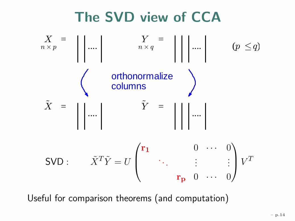
The SVD view of CCA

)(

=....

=....

=....

=....

snmulocezilamronohtro

SVD : XT Y = U

⎛⎜⎝

r1 0 · · · 0. . .

......

rp 0 · · · 0

⎞⎟⎠V T

Useful for comparison theorems (and computation)

– p.14

Example: First use of CCA

“Regressions between Sets of Variables”, F.V. Waugh,Econometrica, 1942

X =“wheat characteristics” Y =“flour characteristics”

x1 = kernel texture y1 = wheat per bbl. of flourx2 = test weight y2 = ash in flourx3 = damaged kernels y3 = crude protein in flourx4 = foreign material y4 = gluten quality indexx5 = crude protein in wheat

aTx index of wheat quality bT y index of flour quality

GOAL: highly correlated grading of raw & finished products

p = 5 q = 4 n = 138

– p.15

Example

Barnett & Preisendorfer, (1987), Monthly Weather Review

Y variables: surface air tem-peratures at 33 U.S. locations;monthly data, 1931-1980

X variables: sea surfacetemp(SST) in 21 regions for3 prior months in 2 seasons.

p = 126 q = 33 n = 600

– p.16

Neglect of CCA in STAT?

Title/Abstract/Keyword search:articles published in 15 mos. in 2002-03:[ISI Web of Science]

Keyword Stat/Prob Other TotalJournals Journals

Canonical 7 116 123Correlation

Gibbs 49 52 101Sampler

– p.17

Recent Variants

Functional CCA Leurgans, Moyeed, Silverman 94Curve data {Xi(t), Yi(t), i = 1, . . . , n} t ∈ Tp = q = # discretization points tk, maybe large

→ regularized CCA: max (aT ΣXY b)2

aT (ΣXX+λD4)a bT (ΣY Y +λD4)b

Kernel ICA Bach, Jordan ’02From yi = Axi, i = 1, . . . , n estimate A. If A is 2× 2(here), set

X =

⎡⎢⎣

Φ(x11)

...

Φ(xn1 )

⎤⎥⎦ Y =

⎡⎢⎣

Φ(x12)

...

Φ(xn2 )

⎤⎥⎦ Φ : R→ F feature sp.

p = q = dim(F) large

→ regularized CCA on X,Y (. . . )

[cf. Renyi (59) ρ∗(X1, X2) = maxθ,φ corr[θ(X1), φ(X2)])– p.18

Agenda

• Orientation






– p.19

Roots of a Determinantal Equation

The equation |XT Y (Y T Y )−1Y T X − r2XT X| = 0becomes

|A− r2(A + B)| = 0where

A = XTPX P = Y (Y T Y )−1Y T

B = XT P⊥X P⊥ = I − P

– p.20

Roots of a Determinantal Equation

The equation |XT Y (Y T Y )−1Y T X − r2XT X| = 0becomes

|A− r2(A + B)| = 0where

A = XTPX P = Y (Y T Y )−1Y T

B = XT P⊥X P⊥ = I − P

Stochastic model: [X : Y ]n×(p+q)

∼ N(0, In ⊗(

ΣXX ΣXY

ΣY X ΣY Y

))

Null distribution: ΣXY = 0 ↔ ρ1 = . . . = ρp = 0

In this case (transforming to ΣXX = I)

A ∼Wp(q, I)

B ∼Wp(n− q, I)independent, Wishart

– p.20

Basic Setting

A ∼Wp(q, I)

B ∼Wp(n− q, I)2 independent Wisharts p ≤ q, n−q

[Recall: if Z has rows zTi

ind∼ Np(0,Σ), then

ZT Z =∑n

i=1 zizTi ∼Wp(n,Σ) ]

Multivariate Beta roots := (ui)pi=1

det[u(A + B)−A] = 0

�Multivariate F roots := (wi)

pi=1

det[wB − A] = 0

Largest Root test: based on u1(≥ u2 ≥ . . . up)

– p.21

Related Classical Problems

2 Wishart setting central to classical multivariate analysis:

• Multiple Response Linear Model

Yn×p

= Xn×q

βq×p

+ En×p

, E ∼ N(0, In ⊗Σ)

Largest root test of H0 : β = 0 uses u1.

• Multiple Discrimination

q populations; n observations on p variables.A and B: between and within class covariance matrices.

• Testing Equality of Two Covariance Matrices

– p.22

From CCA to Other Settings

Basic setting: u1 largest root of det[u(A + B)−A] = 0

CCA [X Y ] ∼ Np+q(0, In ⊗ Σ) p q n− qH0 : ΣXY = 0

Multivariate Y = Xβ + En×p p×q q×p

r g n− q

Linear ↑ ↑ ↑Model H0 : C β M

g×q q×p p×r= 0 dimen hypoth. d.f. error d.f.

Equality niΣi ∼Wp(ni,Σi) p n1 n2

of Covariance H0 : Σ1 = Σ2

Mult. ni obs on q pops p q − 1 n− qDiscrim. Np(µi,Σ)

i = 1, . . . , q– p.23

Agenda

• Orientation






– p.24

Why non-standard asymptotics?

Large literature on det[A− u(A + B)] = 0.Books: e.g. Anderson(58,02); Muirhead(82)

Exact distributions are complex; ∃ much asymptotics withp, q fixed, n→∞

BUT, some results not“numerically available”:e.g. null distribution of largest root u1

nu1 → largest root of Wp(q, I) [finite LOE]

⇒ here, aim for simple approximations from large

(p, q(p), n(p)) asymptotics as p→∞

– p.25

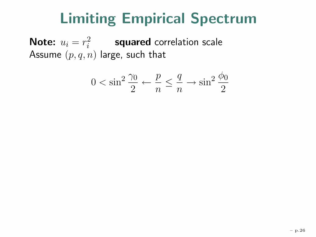
Limiting Empirical Spectrum

Note: ui = r2i squared correlation scale

Assume (p, q, n) large, such that

0 < sin2 γ0

2← p

n≤ q

n→ sin2 φ0

2

– p.26

Limiting Empirical Spectrum

Note: ui = r2i squared correlation scale

Assume (p, q, n) large, such that

0 < sin2 γ0

2← p

n≤ q

n→ sin2 φ0

2

Then (Wachter, 1980)

Fp(u) = p−1#{i : ui ≤ u} →∫ u

0f(u′)du′

f(u) =cu

√(µ+ − u)(u− µ−)

u(1− u)cu = 2π sin2 γ0/2

µ± = cos2(π2 − φ0±γ0

2 )

– p.26

Examples

p q n γ0/2 φ0/2 µ− µ+

10 20 100 .325 .466 .020 .505

50 50 150 .616 .617 .000 .890

4 5 137 .182 .210 .0004 .140

0 0.1 0.2 0.3 0.4 0.5 0.6 0.7 0.8 0.90

2

4

6

8

10

12

– p.27

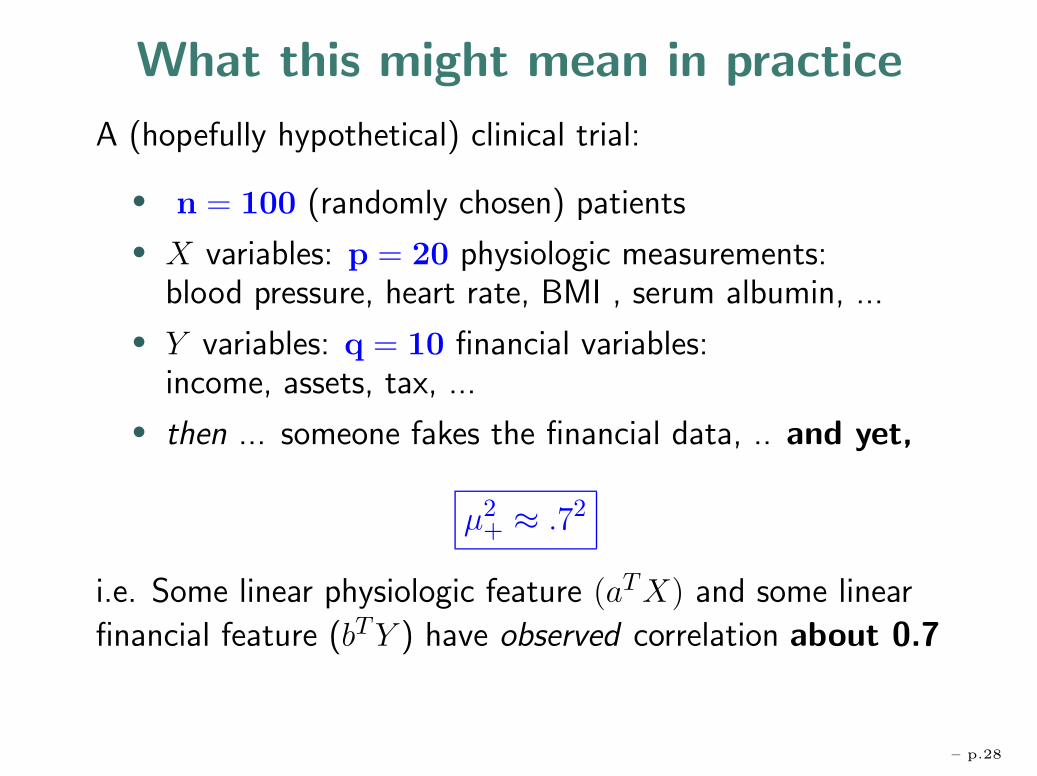
What this might mean in practice

A (hopefully hypothetical) clinical trial:

• n = 100 (randomly chosen) patients

• X variables: p = 20 physiologic measurements:blood pressure, heart rate, BMI , serum albumin, ...

• Y variables: q = 10 financial variables:income, assets, tax, ...

• then ... someone fakes the financial data, .. and yet,

µ2+ ≈ .72

i.e. Some linear physiologic feature (aTX) and some linear

financial feature (bT Y ) have observed correlation about 0.7

– p.28

Agenda

• Orientation






– p.29

Approximate Law for Largest Root

Assume 2 Wishart Setting with p, q(p), n(p)→∞.

γp

2= sin−1

√p

n,

φp

2= sin−1

√q

n.

µ± = cos2(π

2− φp ± γp

2

), σ3

p+ =1

(2n)2sin4(φp + γp)

sin φp sin γp.

– p.30



γp

2= sin−1

√p

n,

φp

2= sin−1

√q

n.

µ± = cos2(π

2− φp ± γp

2

), σ3

p+ =1

(2n)2sin4(φp + γp)

sin φp sin γp.

Theorem (IMJ + Peter Forrester)

P{u1 ≤ s} = P{µ+ + σ+W1 ≤ s}+ o(1)

W1 follows the Tracy-WidomF1 distribution.

-4 -2 2 4

0.05

0.1

0.15

0.2

0.25

0.3

– p.30

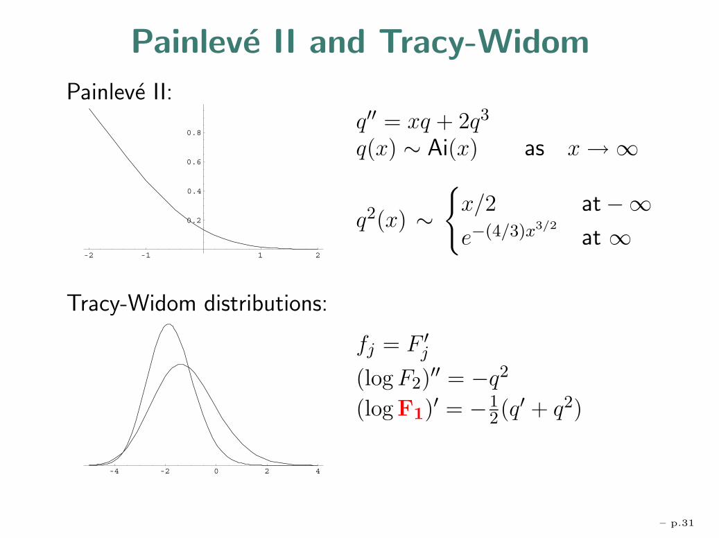
Painleve II and Tracy-Widom

Painleve II:

-2 -1 1 2

0.2

0.4

0.6

0.8

Tracy-Widom distributions:

-4 -2 0 2 4

q′′ = xq + 2q3

q(x) ∼ Ai(x) as x→∞

q2(x) ∼{

x/2 at−∞e−(4/3)x3/2

at ∞

fj = F ′j

(log F2)′′ = −q2

(log F1)′ = −12(q′ + q2)

– p.31



γp

2= sin−1

√p−.5

n−1,

φp

2= sin−1

√q − .5

n− 1.

µ± = cos2(π

2− φp ± γp

2

), σ3

p+ =1

(2n− 2)2sin4(φp + γp)

sin φp sin γp.

Main ‘Result’ (IMJ + Peter Forrester)

P{u1 ≤ s} = P{µ+ + σ+W1 ≤ s}+ O(p−2/3).

• small corrections (.5,1,2) greatly improve approximationfor p, q small, so

• error is O(p−2/3) [ instead of O(p−1/3)]

– p.32

Agenda

• Orientation






– p.33

TW (p, q, n) approximation

Use µ+(p, q, n) + σ+(p, q, n)F1,α

(with F1,α = αth percentile of F1)

to approximate αth percentile of u1

Claim: As a rough guide, the TW-approximation

• mostly mimics tables where extant

• extends tables if not

• improves on some software (S/SPLUS/R; SAS)

– p.34

Approximation vs. Tables for p = 5

Tables: William Chen, IRS,

(2002)

mc =q − p− 1

2∈ [0, 15],

nc =n− q − p− 1

2∈ [1, 1000]

0 5 10 150

0.1

0.2

0.3

0.4

0.5

0.6

0.7

0.8

0.9

1

mc

Squ

ared

Cor

rela

tion

nc = 2

Table vs. Approx at 95th %tile; mc = (q−p−1)/2; nc = (n−q−p−1)/2

nc = 5

nc = 10

nc = 20

nc = 40

nc = 100

nc = 500

Tracy−WidomChen Table p=5

– p.35

Upper Bound in SAS

Approximate n−qq

u1

1−u1by Fq,n−q

0 5 10 150

0.1

0.2

0.3

0.4

0.5

0.6

0.7

0.8

0.9

1

mc

Squ

ared

Cor

rela

tion

nc = 2

Table vs. Approx at 95th %tile; mc = (q−p−1)/2; nc = (n−q−p−1)/2

nc = 5

nc = 10

nc = 20

nc = 40

nc = 100

nc = 500

Tracy−WidomChen Table p=5SAS F−approx

– p.36

Finite (p, q, n) simulations of u1 = r21

p = 20, q = 40,n = 200

Y− axis: quantiles ofsimulated u1 = r2

1

(10, 000 reps.)

X− axis: quantiles ofµ+ + σ+W1

0.35 0.4 0.45 0.5 0.55 0.60.35

0.4

0.45

0.5

0.55

0.6

1%

95% 99%

1%

95% 99%

quantiles of Tracy−Widom Approximation

quan

tiles

of s

imul

ated

squ

ared

cor

rela

tions

1%

95% 99%

qqplot for p=20, q=40, n = 200

1%

95% 99%

20 40 200ur

– p.37

ctd.

TW- Percentile p, q, n 20,40,200

for W1 (µ, σ) (.494, .024)

-3.90 .01 .010

-3.18 .05 .052

-2.78 .10 .104

-1.91 .30 .311

-1.27 .50 .507

-0.59 .70 .706

0.45 .90 .904

0.98 .95 .950

2.02 .99 .990

E.g. .904 = P[u1 − µ+

σ+≤ 0.45 | (p, q, n) = (20, 40, 200)

]– p.38

ctd.

TW- Percentile p, q, n 20,40,200 5,10,50 2,4,20 2 * SE

for W1 (µ, σ) (.494, .024) (.478, .061) (.442, .117)

-3.90 .01 .010 .008 .000 (.002)

-3.18 .05 .052 .049 .009 (.004)

-2.78 .10 .104 .099 .046 (.006)

-1.91 .30 .311 .304 .267 (.009)

-1.27 .50 .507 .506 .498 (.010)

-0.59 .70 .706 .705 .711 (.009)

0.45 .90 .904 .910 .911 (.006)

0.98 .95 .950 .955 .958 (.004)

2.02 .99 .990 .992 .995 (.002)

E.g. .904 = P[u1 − µ+

σ+≤ 0.45 | (p, q, n) = (20, 40, 200)

]– p.39

Remarks

• p−2/3 scale of variability for u1

• 95th %tile.= µp+ + σp+, 99th %tile

.= µp+ + 2σp+

• if µp+ > .7, logit scale vi = log ui/(1− ui) better:

µv+ = logµp+

1− µp+, σv+ = v′(µp+)σp+ =

σp+

µp+(1− µp+)

• Smallest eigenvalue: with previous assumptions and

γ0 < φ0, σ3p− = 1

(2n−2)2sin4(φp−γp)sin φp sin γp

then

µp− − up

σp−D→ W1 (W2)

• Corresponding limit distributions for u2 ≥ · · · ≥ uk,up−k ≥ · · · ≥ up−1, k fixed

– p.40

Logit approximation

Percentile TW 50,50,150 5,5,15 2,2,6 2 * SE

(µ, σ) (2.06, .127) (1.93, .594) (1.69, 1.11)

-3.90 .01 .007 .002 .010 (.002)

-3.18 .05 .042 .023 .037 (.004)

-2.78 .10 .084 .062 .074 (.006)

-1.91 .30 .289 .262 .264 (.009)

-1.27 .50 .499 .495 .500 (.010)

-0.59 .70 .708 .725 .730 (.009)

0.45 .90 .905 .919 .931 (.006)

0.98 .95 .953 .959 .966 (.004)

2.02 .99 .990 .991 .993 (.002)

– p.41

Testing Subsequent Correlations

Suppose: ΣXY =

⎡⎢⎣ρ21 0 · · · 0

. . ....

...

ρ2p 0 · · · 0

⎤⎥⎦ p ≤ q, n−p

If largest r correlations are large, test

Hr :ρr+1 = ρr+2 = . . . = ρp = 0?

Comparison Lemma (from SVD interlacing)

L(ur+1|p, q, n;SXY ∈ Hr)st< L(u1|p, q − r, n; I)

⇒ conservative P−values for Hr via

TW (p, q − r, n) approx’n to RHS

[Aside: L(u1|p− r, q − r, n; I) may be better, but no bounds]– p.42

World Wheats Data ctd.

p = 4 flour characteristics r21 = .923

q = 5 wheat characteristics r22 = .554

n = 137 r23 = .056

r24 = .008

r21 significant (also by permutation test)

r22? 99%−tile of TW (p, q − 1, n) = TW (4, 4, 137)

.= µ + 2σ

.= 0.152� 0.554 = r2

2

→ r22 significant (possible collinearity ... )

– p.43

Agenda

• Orientation






– p.44

Joint distribution of latent roots, 1939

Fisher

Cambridge

Girshick

Columbia

Hsu

London

Mood

Princeton

Roy

Calcutta

f(x) = c

N∏i=1

(1− xi)(α−1)/2(1 + xi)

(β−1)/2∏i<j

|xi − xj|

2 Wishart setting, but notation change:

xi = 2ui− 1, i = 1, . . . , N = p; α = n− q− p;β = q− p

– p.45

Random Matrix Theory

E.g. for largest eigenvalue: hard to marginalize to get atP{l1 ≤ x}.Key role: determinants, not independence:∏

i<j

(li − lj) = det[lk−1i ]1≤i,k≤p

p∏i=1

I{li ≤ x} =

p∑k=0

(−1)k(

p

k

) k∏i=1

I{li > x}.

⇒ P{l1 ≤ x} via Fredholm determinants.

– p.46

Correlation kernel

For complex data Xkl + iX ′kl, joint density f(x1, . . . , xN )

cN∏1

w(xi)∏i<j

(xi − xj)2 =

1

N !det

1≤i,j≤N[KN2(xi, xj)]

with correlation kernel KN2(x, y) =∑N−1

k=0 φk(x)φk(y)

φk(x) = h−1/2k w1/2(x)pk(x) – orthonormalized polynomials, in

classical cases:

w(x) pk(x) Distribution

e−x2/2 Hermite Hk(x) Gaussian

e−xxα Laguerre Lαk (x) Wishart

(1− x)α(1 + x)β Jacobi Pα,β(x) Multivariate Beta

– p.47

Convergence of Kernels (i)

Airy kernel associated with T-W law F2 (T-W, 1994)

KA(s, t) =Ai(s)Ai′(t)− Ai′(s)Ai(t)

s− t

Approach: Uniform convergence of rescaled kernel

σNKN (µN + σNs, µN + σN t)→ KA(s, t) (∗)implies that of extreme eigenvalues (Soshnikov, 01)

L(x(1), . . . , x(k)|FN )→ L(x(1), . . . , x(k)|F2) fixed k

Key point: Choose µN , σN so that error in (*) drops from

O(N−1/3) to O(N−2/3).– p.48

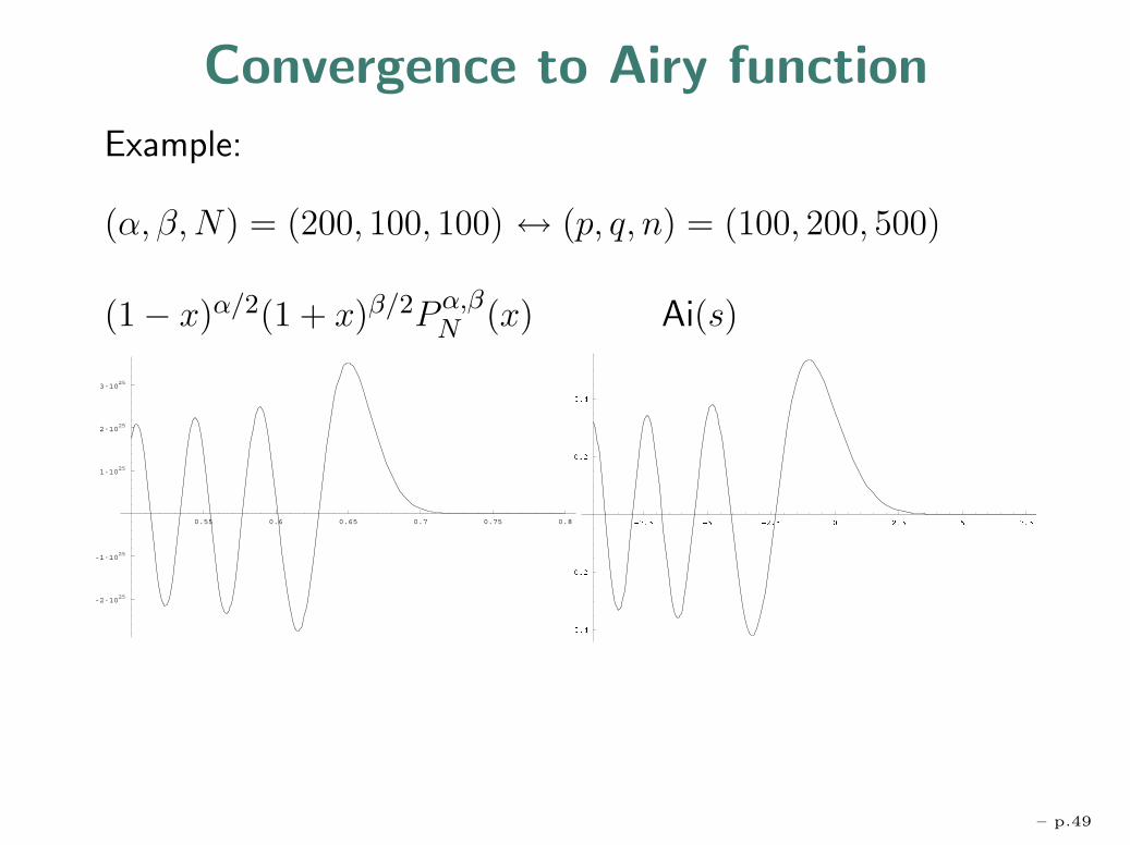
Convergence to Airy function

Example:

(α, β,N) = (200, 100, 100) ↔ (p, q, n) = (100, 200, 500)

(1− x)α/2(1 + x)β/2Pα,βN (x) Ai(s)

0.55 0.6 0.65 0.7 0.75 0.8

-2·1025

-1·1025

1·1025

2·1025

3·1025

– p.49

Convergence of Kernels (ii)

Jacobi polynomials Pα,βN satisfy differential equation

W ′′(x) = {κ2f(x) + g(x)}W (x)

• treble asymptotics: (α, β,N) = (n− p− q, q − p, p) large

• Airy approximation at largest zero [Liouville-Green/WKB]

• Error Bounds Olver, 74 constrain κ, f, g and yield error

O(N−2/3).

Real Case:

• quaternion determinants

• closed form formulas: Adler-Forrester-Nagao-vanMoerbeke

• ’miraculous’ cancellations → O(N−2/3)– p.50

Agenda

• Orientation






– p.51

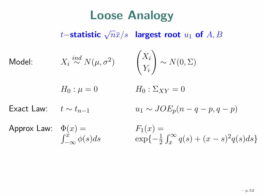
Loose Analogy

t−statistic√

nx/s largest root u1 of A,B

Model: Xiind∼ N(µ, σ2)

(Xi

Yi

)∼ N(0,Σ)

H0 : µ = 0 H0 : ΣXY = 0

Exact Law: t ∼ tn−1 u1 ∼ JOEp(n− q − p, q − p)

Approx Law: Φ(x) = F1(x) =∫ x−∞ φ(s)ds exp{−1

2

∫∞x q(s) + (x− s)2q(s)ds}

– p.52

Loose Analogy

t−statistic√

nx/s largest root u1 of A,B

Model: Xiind∼ N(µ, σ2)

(Xi

Yi

)∼ N(0,Σ)

H0 : µ = 0 H0 : ΣXY = 0Exact Law: t ∼ tn−1 u1 ∼ JOEp(n− q − p, q − p)Approx Law: Φ(x) = F1(x) =∫ x

−∞ φ(s)ds exp{−12

∫∞x q(s) + (x− s)2q(s)ds}

Second-Order Accuracy Correlation functions

P{tn−1 ≤ x} = Φ(x) + O[(

1√n

)2]σNKN (µN + σNs, µN + σN t)

→ KA(s, t) + O(N−2/3)

Claim: P{u1 ≤ µN + σNx}= F1(x) + O(N−2/3)

– p.53

Non Gaussian Data

– p.54

Agenda

• Orientation





– p.55

Ex. 3: PCA - Estimating Eigenvectors

High-p signal processing areas, e.g.

hyperspectral data, face recognition, ECGs

routinely use dimensionality reduction techniques

variable/feature selection, PCA, transform domains

Combined (in some order) to aim for sparse representation,e.g.:

• transform to wavelet basis (dimension n)

• select high variance variables (dimension k � n)

• PCA on reduced subset (O(k3) vs. O(n3))

Clear speed benefits; here: helps with consistency issues

– p.56

Orthogonal Factor models in PCA

xi = µ + viρ + σzi i = 1, . . . , n

• ρ ∈ Rp, single component to be estimated

• vii.i.d.∼ N(0, 1) random effects

• zii.i.d.∼ Np(0, I) Gaussian noise (e.g. σ = 1)

– p.57

Orthogonal Factor models in PCA

xi = µ + viρ + σzi i = 1, . . . , n

• ρ ∈ Rp, single component to be estimated

• vii.i.d.∼ N(0, 1) random effects

• zii.i.d.∼ Np(0, I) Gaussian noise (e.g. σ = 1)

A Multicomponent Model

xi =m∑

j=1

vji ρ

j + σzi, i = 1, . . . , n

ρj unknown, orthogonal, ‖ρ1‖ ≥ · · · ≥ ‖ρm‖; for asymptotics

(‖ρ1(n)‖, . . . , ‖ρj(n)‖, . . .) �1→ (�1, . . . , �j , . . .).

– p.57

Inconsistency

In either single (or multi-) component model,

Theorem (Lu) If p/n→ c > 0, then

lim infn→∞ E sin ∠(ρ, ρ) > 0.

• Noise does not average out in PCA if too manydimensions p relative to n.

• Suggests: reduce p to k � p before starting PCA

– p.58

Sparsity and PCA

In basis {eν(t)}, a population p.c. {ρ} has coefficents {ρν}:

ρ(t) =

p∑ν=1

ρνeν(t).

Sparsity and weak �p Say ρ ∈ w�p(C) if

|ρ(ν)| ≤ Cν−1/p, ν = 1, 2, . . .

• p small ⇒ rapid decay of ordered coefficients

• choose basis to exploit sparsity

– p.59

Consistency of Sparse PCA

• Single component model. Suppose (i) p/n→ c > 0,(ii) ‖ρ(n)‖ → � > 0.

• Assume Sparsity : ρ(n) ∈ w�p(C) uniformly in n

• Subset selection rule:

I = {ν : σ2ν > σ2(1 + c

√2 log p

√2/n)}

• Let ρ denote sparse PCA estimate based on I.

Theorem ∠(ρ, ρ)a.s.→ 0.

Later work (D. Paul): rates of convergence, lower bounds.

– p.60

Example 3: Summary for Sparse PCA

• initial dimension reduction before PCA• otherwise, inconsistency!

• use basis with sparse representation• so that little is lost in initial dimension reduction

• Background role for large random matrices• Small perturbations of symmetric matrices• a.s. bounds for extreme eigenvalues of large matrices

– p.61

Agenda

• Orientation





– p.62

Some Related Problem Areas• Extreme Sample Eigenvalues in large n, p setting.• Limiting distributions and approximations under

“alternative”hypotheses• First order (strong law behavior) under dependence• Validity of bootstrap confidence intervals

– p.63



• Sample Eigenvectors (associated with extremeeigenvalues)• Consistency and asymptotic distribution as p grows• Effect of regularization (as in functional data)• possibilities for“sparse”versions of PCA [Lu]

– p.63



• Sample Eigenvectors (associated with extremeeigenvalues)• Consistency and asymptotic distribution as p grows• Effect of regularization (as in functional data)• possibilities for“sparse”versions of PCA [Lu]

• Empirical distributions of eigenvalues• (further) statistical uses of Marcenko-Pastur law• statistical potential of central limit theorems for

linear statistics of eigenvalues∑

h(li).– p.63

Some Related Problem Areas, Ctd.• Estimation of large covariance matrices• Sparsity models for non-unit variances (subspaces of

elevated variance)• Prior distributions on covariance matrices• Frequentist properties of Bayes estimates

– p.64



• Classification & clustering• kernel PCA and ICA in statistical learning theory• models for large covariance structures

– p.64



• Classification & clustering• kernel PCA and ICA in statistical learning theory• models for large covariance structures

• Issues from application domains• meteorology/climate, signal processing (multiple

input, multiple output (MIMO)), face recognition,document retrieval, hyperspectral imagery

– p.64

Publicity

Program, Fall Semester 2005-06, atSAMSI [Statistics and Applied MathS Institute], North Carolina

“High dimensional multivariate statistics and randommatrices”

• statistical focus: spectral properties – eigenvalues,eigenvectors

• RMT focus: RMT applications with (potential)relevance to statistics

• connections with selected areas of application

Info: contact IMJ or Craig Tracy (UC Davis)

– p.65

THANK YOU!

– p.66

large covariance matrices - home | department of...

Documents