testing hypotheses about covariance matrices in general

Statistica Sinica

Testing Hypotheses about

Covariance Matrices in General MANOVA Designs

Paavo Sattler1, Arne Bathke2 and Markus Pauly1

1TU Dortmund University and 2University of Salzburg

Abstract

We introduce a unified approach to testing a variety of rather gen-

eral null hypotheses that can be formulated in terms of covariances

matrices. These include as special cases, for example, testing for

equal variances, equal traces, or for elements of the covariance ma-

trix taking certain values. The proposed method only requires very

few assumptions and thus promises to be of broad practical use.

Two test statistics are defined, and their asymptotic or approximate

sampling distributions are derived. In order to particularly im-

prove the small-sample behavior of the resulting tests, two bootstrap-

based methods are developed and theoretically justified. Several

simulations shed light on the performance of the proposed tests.

The analysis of a real data set illustrates the application of the pro-

cedures.

Keywords: Bootstrap, Multivariate Data, Nonparametric Test, Resampling, Trace.

arX

iv:1

909.

0620

5v3

[m

ath.

ST]

22

Dec

202

0

1. MOTIVATION AND INTRODUCTION

It is of substantial interest to have valid statistical methods for inference on co-

variance matrices available for at least two major reasons. The first one is that

a treatment effect may indeed best be described by a particular configuration of

scale or covariance parameters – not by a mean difference. The second reason cor-

responds to a more indirect purpose, namely that the main interest of the investi-

gation may be described by a location change under the alternative, but some of

the available inference methods for location effects rely on assumptions regarding

variances or covariances that need to be assessed reliably. In either situation, a sta-

tistical test about hypotheses that are formulated in terms of covariance matrices

is necessary. From a methodological point of view, such a test shall not make too

many restrictive assumptions itself, for example, regarding underlying distribu-

tions. Furthermore, it shall perform well for moderate sample sizes, where clearly

the term moderate will have to be seen in connection with the number of parameters

effectively being tested.

Considering the central importance and the widespread need for hypothesis tests

on covariance matrices, it may come as a surprise that a general and unifying ap-

proach to this task has not been developed thus far. There are several tests for

specialized situations, such as testing equality of variances or even covariance

matrices. Many of these approaches will be mentioned below. However, they

typically only address one particular question, and they often rely on restrictive

distributional assumptions, such as normality (e.g. in Box (1953) and Anderson

(1984)), elliptical distributions (e.g. in Muirhead (1982), Fang and Zhang (1990)

and Hallin and Paindaveine (2009)), or conditions on the characteristic functions

(e.g. in Gupta and Xu (2006)).

One exception is the test of Zhang and Boos (1993), which theoretically allows

for testing a multitude of hypotheses without restrictive distributional conditions.

Unfortunately, this procedure’s small and medium sample performance is com-

paratively poor, particularly regarding the power. Their technique to improve the

performance requires a more restrictive null hypothesis that additionally postu-

lates equality of certain moments. This makes it somewhat difficult to use this

approach in practice, as rejection does not mean that the covariances are unequal.

The goal of the present article is to introduce a very general approach to statistical

hypothesis testing, where the hypotheses are formulated in terms of covariance

matrices. This includes as special cases, for example, hypotheses formulated us-

ing their traces, hypotheses of equality of variances or of covariance matrices, and

hypotheses in which a covariance matrix is assumed to have particular entries.

The test procedures are based on a resampling approach whose asymptotic va-

lidity is shown theoretically, while the actual finite sample performance has been

investigated through extensive simulation studies. Analysis of a real data example

illustrates the application of the proposed methods.

In the following section, the statistical model and (examples for) different null hy-

potheses that can be investigated using the proposed approach will be introduced.

Thereafter, the asymptotic distributions of the proposed test statistics are derived

(Section 3) and proven to be regained by two different resampling strategies (Sec-

tion 4). The simulation results regarding type-I-error control and power are dis-

cussed in Section 5, computation time is considered in Section 6, while an illustra-

tive data analysis of EEG-data is conducted in Section 7. All proofs are deferred to

a technical supplement.

2. STATISTICAL MODEL AND HYPOTHESES

We consider a general semiparametric model given by independent d-dimensional

random vectors

Xik = µi + εik. (2.1)

Here, the index i = 1, . . . ,a refers to the treatment group and k = 1, . . . ,ni to the

individual, on which d-dimensional observations are measured. More details to

this model can be found in the supplementary material.

In this setting, E(Xik) = µi = (µi1, . . . ,µid)> ∈ Rd denotes the i-th group mean

while the residuals εi1, . . . ,εini are assumed to be centered E(εi1) = 0 and i.i.d.

within each group. We require finite fourth moment E(||εi1||4) <∞, where this de-

notes the Euclidean norm. However, beyond this, there are no other distributional

assumptions. In particular, the covariance matrices Cov(εi1) = Vi > 0 may be

arbitrary and do not even have to be positive definite. For convenience, we aggre-

gate the individual vectors into X = (X>11, . . . ,X>ana)> as well as µ = (µ>1 , . . . ,µ>a )>.

Stacking the covariance matrix Vi = (virs)dr,s into the p := d(d+ 1)/2-dimensional

vector vi = vech(Vi) = (vi11, vi12, . . . , vi1d, vi22, . . . , vi2d, . . . , vidd)> (i = 1, . . . ,a)

containing the upper triangular entries of Vi we formulate hypotheses in terms of

the pooled covariance vector v = (v>1 , . . . , v>a )> as

Hv0 : Cv = ζ. (2.2)

Here, C denotes a suitable hypothesis matrix of interest, and ζ is a fixed vector. It

should be noted that we don’t assume that C is a contrast matrix, not to mention

a projection matrix. This is different from the frequently used hypothesis formula-

tion about mean vectors in MANOVA designs (Konietschke et al. (2015), Friedrich

et al. (2017), Bathke et al. (2018)), where one can usually work with a unique pro-

jection matrix. However, working with simpler matrices (as we do) can help to

save considerable computation time, see Remark 1 below.

In order to discuss some particular hypotheses included within the general setup

(2.2), we fix the following notation: Let Id be the d-dimensional unit matrix, 1d =

(1, . . . , 1)> the d-dimensional column vector of 1’s and Jd = 1d1>d the d-dimensional

matrix of 1’s. Furthermore, Pa = Ia − Ja/a denotes the a-dimensional centering

matrix, while ⊕ and ⊗ denote direct sum and Kronecker product, respectively.

Then the following null hypotheses of interest are covered:

(a) Testing equality of variances: For a univariate outcome with d = 1, testing the

null hypothesis Hv0 : v111 = v211 = · · · = va11 of equal variances is included within

(2.2) by setting C = Pa and ζ = 0. Hypotheses of this type have been studied

by Bartlett and Rajalakshman (1953) as well as Boos and Brownie (2004), Gupta

and Xu (2006), and Pauly (2011), among others. In the special case of a two-armed

design with a = 2, this is also the null hypothesis inferred by the popular F-ratio

test which, however, is known to be sensitive to deviations from normality (Box

(1953)).

(b) Testing for a given covariance matrix: Let Σ be a given covariance matrix. It

may represent, for example, an autoregressive or compound symmetry covariance

structure. For a = 1, our general formulation also covers testing the null hypothe-

sis Hv0 : V1 = Σ by setting C = Ip and ζ = vech(Σ). Hypotheses of this kind have

been studied by Gupta and Xu (2006).

(c) Testing homogeneity of covariance matrices: More general than in (a), let

C = Pa⊗Ip and ζ = 0 for arbitrary d ∈ N. Then (2.2) describes the null hypothesis

Hv0 : V1 = · · · = Va. For multivariate normally distributed random variables, this

is the testing problem of Box’s-M-test Box (1953), for which extensions have been

studied in Lawley (1963), Browne and Shapiro (1986), Zhu et al. (2002), and Yang

and DeGruttola (2012). Moreover, Zhang and Boos (1992, 1993) proposed Bartlett-

type tests with bootstrap approximations in a general model similar to ours. How-

ever, the pooled bootstrap method of Zhang and Boos (1992) requires equality of

some special kind of fourth moments across groups while the separate bootstrap

approximation proposed in Zhang and Boos (1993) exhibited unsatisfactory small

sample behavior in terms of size control or power.

Beyond the above choices, Hv0 in (2.2) even contains hypotheses about linear func-

tions of matrices. To this end, set hd := (1, 0>d−1, 1, 0>d−2, . . . , 1, 0, 1)> and consider

the following examples:

(d) Traces as effect measures: Suppose we are interested in the total variance∑d`=1 Var(Xi1`) = tr(Vi) of all components as a univariate effect measure for each

group. This may be an advantageous approach in terms of power, as illustrated in

the data example analysis below. Then, their equality Hv0 : tr(V1) = · · · = tr(Va)

can be tested by choosing C = Pa ⊗ [hd · h>d ]/d, and ζ = 0

(e) Testing for a given trace: Consider the situation of example (d) with just one

group a = 1. We then may be interested in testing for a given value γ ∈ R of the

trace, i.e. Hv0 : tr(V1) = γ. Therefore we chose C = e1 · h>d and ζ = e1 · γ, with

e1 = (1, 0>d−1)>.

(f) Higher Way Layouts: Moreover, we can even infer hypotheses about variances,

covariance matrices, or traces in arbitrarily crossed multivariate layouts by split-

ting up indices. For example, consider a two-way cross-classified design with fixed

factors A and B whose levels are i1 = 1, . . . ,a and i2 = 1, . . . ,b, respectively. As-

sume that the interest lies in measuring, for example, their effect on the total vari-

ance, that is, the trace (a similar approach works for variances and covariances).

We observe ni1i2 > 0 subjects for each factor level combination (i1, i2). To formu-

late hypotheses of no main trace effects for each factor, as well as hypotheses of

no interaction trace effects we write tr(Vi1i2) = t + αi1 + βi2 + (αβ)i1i2 with the

usual side conditions∑i1αi1 =

∑i2βi2 =

∑i1(αβ)i1 =

∑i2(αβ)i2 = 0. Here,

for example, αi1 can be interpreted as the part of the total variance under factor

level i1 by factor A. Then, the choice C = (Pa ⊗ Jb/b) ⊗ (hd · h>d/d) and ζ = 0

leads to a test for no main effect of factor A (measured in the above trace effects),

Hv0 : α1 = · · · = αa = 0, while C = (Pa ⊗ Pb)⊗ (hd · h>d/d) and ζ = 0 result in the

hypothesis of no interaction (again measured in trace effects) between the factors

A and B, Hv0 : αβij ≡ 0 for all i, j.

Remark 1. Although in most of the considered scenarios, it is possible to find an

idempotent symmetric hypothesis matrix C, the option ζ 6= 0p allows for matri-

ces that are neither symmetric nor idempotent. From a theoretical point of view,

this does not really matter. However, from a practical point of view, the choice

of the hypothesis matrix may actually have a great effect with regard to saving

computation time. To this aim, we allow C ∈ Rm×ap with m 6 ap together with

appropriate ζ ∈ Rm and formulate all our theorems for this kind of matrices. For

example Hv0 : tr(V1) = γ could also be formulated by h>d · v = γ. Depending on

the hypothesis of interest, the computational savings in our simulations were up

to 66% for smaller dimensions and partially even more than 99% for larger dimen-

sions, see Section 6.1 for a detailed discussion.

In the subsequent sections, we develop testing procedures for Hv0 in (2.2) and thus

for all given examples (a)–(f) above. The basic idea is to use a quadratic form in

the vectorCv̂−ζ of estimated and centered effects. For ease of presentation and its

widespread use in our setting (with E(||εi1||4) <∞), we thereby focus on empirical

covariance matrices V̂i = (ni − 1)−1 ∑nik=1(Xik−Xi·)(Xik−Xi·)

>, v̂i = vech(V̂i),

as estimators for Vi, i = 1, ...,a, where Xi· = ni−1 ∑nik=1Xik. Other choices, as, for

example, surveyed in Duembgen et al. (2013), may be part of future research.

Thereby, inverting the resulting test procedures will lead to confidence regions about

the effect measures of interest. For example, in case (e), we may obtain confidence

intervals for the unknown trace tr(V1).

3. THE TEST STATISTICS AND THEIR ASYMPTOTICS

In order to obtain the mentioned inference procedures which are formulated using

quadratic forms, we first have to study the asymptotic behaviour of the normalized

m-dimensional vector√N(Cv̂− ζ), where v̂ = (v̂

>1 , . . . , v̂>a )> is the pooled empiri-

cal covariance estimator of v. For convenience, we thereby assume throughout that

the following asymptotic sample size condition holds, as min(n1, . . . ,na)→∞:

(A1) niN→ κi ∈ (0, 1], i = 1, ...,a for N =

∑ai=1 ni.

As κi > 0 holds for all i, we have κ1 = 1 if and only if a = 1. Under this frame-

work, we obtain the first preliminary result towards the construction of proper test

procedures.

Theorem 1. Suppose Assumption (A1) holds. Then, as N→∞, we have convergence in

distribution√NC(v̂− v)

D−→ Nm(0m,CΣC>

),

where Σ =⊕ai=1 κi

−1 · Σi and Σi = Cov(vech(εi1ε>i1)) for i = 1, . . . ,a.

Together with a consistent estimator for (all or certain parts of) Σ, this result will

allow us to develop asymptotic tests for the null hypothesis (2.2). To this end, we

define the empirical estimator Σ̂ :=⊕ai=1N/ni · Σ̂i for Σ, where

Σ̂i =1

ni − 1

ni∑k=1

[vech

(X̃ikX̃

>ik −

ni∑`=1

X̃i`X̃>i`

ni

)][vech

(X̃ikX̃

>ik −

ni∑`=1

X̃i`X̃>i`

ni

)]>.

Here, X̃ik := Xik − Xi· denotes the centered version of observation k in group

i. The consistency of the matrices Σ̂i for Σi and thus of Σ̂ is established in the

supplementary material.

Now potential test statistics may lean on well-known quadratic forms used for

mean-based MANOVA-analyses in heteroscedastic designs (Konietschke et al. (2015),

Bathke et al. (2018)). To unify several approaches we consider

Q̂v = N [Cv̂− ζ]>E(C, Σ̂) [Cv̂− ζ] , (3.3)

where, E(C, Σ̂) ∈ Rm×m is some symmetric matrix that can be written as a function

of the hypothesis matrix C ∈ Rm×ap and the covariance matrix estimator Σ̂ ∈

Rad×ad. In order to analyze the limit behaviour of Q̂v we assume throughout that

E(C, Σ̂) P→ E(C,Σ) holds which is, e.g., fulfilled if E is continuous in its second

argument. Choices covered by this general formulation include the following:

1. An ANOVA-type-statistic (ATS): ATSv(Σ̂) = N [Cv̂− ζ]>[Cv̂− ζ] / tr

(CΣ̂C>

)

corresponding to E(C, Σ̂) = Im/ tr(CΣ̂C>).

2. A Wald-type-statistic (WTS): WTSv(Σ̂) = N [Cv̂− ζ]>(CΣ̂C>

)+[Cv̂− ζ].

Here, E(C, Σ̂) =(CΣ̂C>

)+is the Moore-Penrose-inverse of CΣ̂C>. As we

will see later, the usual χ2f-limit distribution with f = rank(C) will appear

under the additional assumption Σ > 0. This or comparable conditions are

required to garantee E(C, Σ̂) P→ E(C,Σ).

3. Substituting Σ̂ in the WTS with Σ̂0, the diagonal matrix only containing the

diagonal elements of Σ̂, leads to the so-called modified ANOVA-type statis-

tic (MATS) given byMATSv(Σ̂) = N [Cv̂− ζ]>(CΣ̂0C

>)+

[Cv̂− ζ]. To study

its asymptotics we need to assume Σ0 > 0.

In 2. and 3. the additional assumptions are needed to ensure that the inner Moore

Penrose inverse is consistent. The following result establishes the asymptotic dis-

tribution of all quadratic forms of type (3.3) and covers all the cases 1.-3..

Theorem 2. Under Assumption (A1) and the null hypothesis Hv0 : Cv = ζ, the quadratic

form Q̂v defined by (3.3) has, asymptotically, a “weighted χ2-distribution”. That is,

Q̂vD−→

ap∑`=1

λ`B`,

where B`i.i.d.∼ χ2

1 and λ`, ` = 1, . . . ,ap, are the eigenvalues of (Σ1/2C>E(C,Σ)CΣ1/2).

This result allows the definition of a natural test procedure in the WTS given by

ϕWTS = 11{WTSv(Σ̂) /∈ (−∞,χ2f;1−α]}. However, the additional condition Σ > 0,

ensuring asymptotic correctness of ϕWTS, may not always be satisfied in practice.

Since this condition is not needed for the ANOVA-type statistic AN = ATSv(Σ̂),

we focus on the ATS in what follows; noting that the MATS did also show good

finite sample properties in simulations, see the supplement for details. As the limit

distribution of the ATS depends on unknown quantities, we cannot calculate criti-

cal values from Theorem 2 directly. To this end, we employ resampling techniques

for calculating proper critical values. We thereby focus on two resampling proce-

dures: a parametric and a wild bootstrap as both methods have shown favorable

finite sample properties in multivariate mean-based MANOVA (Konietschke et al.

(2015), Friedrich et al. (2016), Friedrich and Pauly (2017), and Zimmermann et al.

(2019)). That these procedures also lead to valid testing procedures in the current

setting is proven in the subsequent section.

4. RESAMPLING PROCEDURES

To derive critical values for the non-pivotal test statistics like ATSv, we consider

two common kinds of bootstrap techniques: a parametric and a wild bootstrap as

applied for heteroscedastic MANOVA. Since we deal with covariances instead of

expectations, some adjustments have to be made in order to prove their asymptotic

correctness.

4.1 Parametric Bootstrap

4.1 Parametric Bootstrap

To motivate our first resampling strategy, note that

√N(v̂i − vi) =

√Nvech

(1

ni − 1

ni∑k=1

[εikε

>ik −Vi

])+OP(1)

D→ Np

(0p, 1

κiΣi

)(4.4)

follows from the proof of Theorem 1.

Thus, to mimick its limit distribution and afterwards the structure of the test statis-

tic, we generate bootstrap vectors Y∗i1, ...,Y∗inii.i.d.∼ Np

(0p, Σ̂i

), for given realisa-

tions Xi1, ...,Xini with estimators Σ̂i. We then calculate Σ̂∗i , the empirical covari-

ance matrix of the bootstrap sample Y∗i1, ...,Y∗ini and set Σ̂∗:=⊕ai=1N/ni · Σ̂

∗i .

The next theorem ensures the asymptotic correctness of this approach.

Theorem 3. Under Assumption (A1), the following results hold:

(a) For i = 1, ...,a, the conditional distribution of√N Y

∗i , given the data, converges

weakly to Np(0p, κi−1 · Σi

)in probability. Since Σ̂

∗i → Σi in probability, the unknown

covariance matrix Σi can be estimated through Σ̂∗i .

(b) The conditional distribution of√N Y

∗, given the data, converges weakly to

Na·p(0a·p,

⊕ai=1 κi

−1 · Σi)

in probability. Since Σ̂∗→ Σ in probability, the unknown

covariance matrix Σ can be estimated through Σ̂∗.

As a consequence, it is reasonable to calculate the bootstrap version of the general

quadratic form (3.3) as Q∗v = N[CY∗]>E(C, Σ̂

∗)[C Y

∗]. For the ATS, e.g., this leads

to ATS∗v = N[CY∗]>[C Y

∗]/

tr(CΣ̂∗C>). The bootstrap versions approximate the

4.2 Wild Bootstrap

null distribution of Q̂v, as established below.

Corollary 1. For each parameter v ∈ Ra·p and v0 withCv0 = ζ, we have under Assump-

tion (A1) that

supx∈R

∣∣Pv(Q∗v 6 x|X) − Pv0(Q̂v 6 x)∣∣ P→ 0,

where Pv denotes the (un)conditional distribution of the test statistic when v is the true

underlying vector.

Denoting with cATS∗,1−α the (1−α)-quantile of the conditional distribution ofATS∗v

given the data, we obtain ϕ∗ATS = 11{ATSv(Σ̂) /∈ (−∞, cATS∗,1−α]} as asymptotic

level α test.

Beyond being helpful to carry out an asymptotic level α test in the ATSv, resam-

pling can also be used to enhance the finite sample properties of the WTSv. In

fact, utilizing Theorem 3 shows that a parametric bootstrap version of the WTSv,

say WTS∗v, is also asymptotically χ2rank(C)-distributed, under the assumption given

in Theorem 1. Thus, it leads to a valid parametric bootstrap WTSv-test as long as

Σi > 0 for all i = 1, . . . ,a.

4.2 Wild Bootstrap

As a second resampling approach, we consider the wild bootstrap. Hereby the

structure of the data is kept more than for the parametric bootstrap since no fixed

distribution is used.In the mean-based analysis, convenient wild bootstrap mul-

tipliers are multiplied with the realizations to get the bootstrap sample. In con-

4.2 Wild Bootstrap

trast, we have to multiply them with p-dimensional random vectors of the kind

vech(XikX>ik), to ensure asymptotic correctness due to (4.4).

Specifically, generate i.i.d. random weights Wi1, ...,Wini , i = 1, ...,a, independent

of the data, with E(Wi1) = 0 and Var(Wi1) = 1. Common choices are for example

standard distributed random variables or random signs. Afterwards the wild boot-

strap sample is defined as Y?ik = Wik ·

[vech(X̃ikX̃

>ik) − n

−1i

∑ni`=1 vech(X̃i`X̃

>i`)],

where again centering is needed to capture the correct limit structure. Defining Σ̂?

i

as the empirical covariance matrix of Y?i1, ...,Y?

iniand setting Σ̂

?=⊕ai=1N/ni · Σ̂

?

i ,

we obtain the following theorem.

Theorem 4. Under Assumption (A1), the following results hold:

(a) For i = 1, ...,a, the conditional distribution of√N Y

?

i , given the data converges weakly

to Np(0p, κi−1 · Σi

)in probability. Since Σ̂

?

i → Σi in probability, the unknown covari-

ance matrix Σi can be estimated through Σ̂?

i .

(b) The conditional distribution of√N Y

?, given the data converges weakly to

Na·p(0a·p,

⊕ai=1 κi

−1 · Σi)

in probability. Since Σ̂?→ Σ in probability, the unknown

covariance matrix Σ can be estimated through Σ̂?.

The result again gives rise to define a wild bootstrap quadratic form

Q?v = N[CY

?]>E(C, Σ̂

?)[C Y

?], where, e.g., an ATSv(Σ̂) wild bootstrap counterpart

is given by ATS?v = N[CY?]>[CY

?]/

tr(CΣ̂?C>). Similar to the parametric boot-

strap, the next theorem guarantees the approximation of the original test statistic

by its bootstrap version.

Corollary 2. Under the assumptions of Corollary 1, we have convergence

supx∈R

∣∣Pv(Q?v 6 x|X) − Pv0(Q̂v 6 x)

∣∣ P→ 0.

Therefore, analogous to ϕ∗ATS, we define ϕ?ATS := 11{ATSv(Σ̂) /∈ (−∞, cATS?,1−α]}

as asymptotic level α test, with cATS?,1−α denoting the (1 − α) quantile of the con-

ditional distribution of ATS?v given the data.

Similar wild bootstrap versions of the WTSv or comparable statistics can again be

defined and used to calculate critical values ifΣ > 0 is fulfilled, see Section 5 below

for the WTS and the supplement for another, less known, possibility.

5. SIMULATIONS

The above results are valid for large sample sizes. For an evaluation of the finite

sample behavior of all methods introduced above, we have conducted extensive

simulations regarding

(i) their ability to keep the nominal significance level and

(ii) their power to detect certain alternatives in various scenarios.

In particular, we studied three different kinds of hypotheses:

A) Equal Covariance Matrices: Hv0 : V1 = V2 with a = 2 groups.

B) Equal Diagonal Elements: Hv0 : V111 = ... = V1dd in the one sample case.

C) Trace Test: Hv0 : tr(V1) = tr(V2) with a = 2 groups.

Each of these hypotheses can be formulated with a proper projection matrix C.

While C(A) = P2 ⊗ Id and C(C) = P2 ⊗ [hd · h>d ]/d follows directly from Section

2, C(B) = diag(hd) − hd · h>d/d is an adaptation of Pd.

For each hypothesis, we have simulated the two bootstrap methods based on the

ANOVA-type statisticϕ∗ATS andϕ?ATS, as well as the Wald-type-statisticϕ∗WTS and

ϕ?WTS. The latter ones are based on the parametric bootstrap version of the WTS,

given by

WTS∗(Σ̂∗) := N

[CY∗]> (

CΣ̂∗C>)+ [

CY∗]

(5.5)

and the wild bootstrap version given by

WTS?(Σ̂?) := N

[CY

?]> (

CΣ̂?C>)+ [

CY?]

. (5.6)

Moreover, the asymptotic version ϕWTS based upon the χ2rank(C)-approximation

serves as another competitor. As additional competitor, we consider a Monte-

Carlo test in the ATS. Recall that its limiting null distribution is given by A0 :=∑mk=1 λkBk

/tr(CΣC>

)for Bk

i.i.d.∼ χ2

1 and λk ∈ eigen(CΣC>

). Plugging in Σ̂ for

Σ and repeatedly generating Ck’s within 10.000 Monte-Carlo of A0, we obtain an

estimated (1 − α)-quantile qMC1−α of the distribution of A0. This finally defines the

Monte-Carlo ATS test ϕATS := 11{ATSv(Σ̂) /∈ (−∞,qMC1−α]}.

In the special case of scenario A), we have also considered the tests from

Zhang and Boos (1992, 1993) based on Bartlett’s test statistic, along with a so-called

separate bootstrap as well as a pooled bootstrap to calculate critical values. We de-

note these tests by ϕB−S and ϕB−P. While the first is asymptotically valid under

the same conditions as our tests, the pooled bootstrap procedure additionally re-

quires E([vech(ε1ε

>1 )] [vech(ε1ε1)

>]>) = E([vech(ε2ε

>2 )] [vech(ε2ε

>2 )]>).

Additionally, we simulated Box’s M-test as it is the most popular test for scenario

A), although it requires normally distributed data. There are two common ways

to determine critical values for this test (Box (1949)): Utilizing a χ2f-approximation

with f = rank(C) degrees of freedom or an F-approximation with estimated de-

grees of freedom. For ease of completeness, we decided to simulate both.

On an abstract level, the hypotheses considered thus far also fall into the frame-

work presented by Zhang and Boos (1993). However, they do not provide concrete

test statistics that we could use for comparison purposes. Other existing tests,

such as the one by Gupta and Xu (2006) rely on rather different model assump-

tions, which also makes a comparative evaluation difficult. All simulations were

conducted by means of the R-computing environment version 3.6.1 R Core Team

(2019) with Nsim = 2 · 104 runs, 1000 bootstrap runs and α = 5%.

Data generation

We considered 5-dimensional observations generated independently according to

the model Xik = µi + V1/2Zik, i = 1, . . . ,a,k = 1, . . . ,ni with µ1 = (12, 22, ..., 52)/4

and µ2 = 05. Here, the marginals of Zik = (Zikj)5j=1 were either simulated inde-

pendently from

• a standard normal distribution, i.e. Zikj ∼ N(0, 1)

• a standardized centered gamma distribution i.e. (√

2Zikj + 2) ∼ G(2, 1)

• a standardized centered skew normal distribution with location parameter

ξ = 0, scale parameterω = 1 and α = 4. The density of a skew normal distri-

bution is given through 2ωφ(x−ξω

)Φ(α(x−ξω

)), where φ denotes the densitiy

of a standard normal distribution andΦ the according distribution function.

For the covariance matrix, an autoregressive structure with parameter 0.6 was cho-

sen, i.e., (V)ij = 0.6|i−j|. More simulation results with different covariance matrices

and more distributions can be found in the supplement. This includes hypotheses

with more groups or settings with a higher dimension of the observations.

Note that the chosen dimension of d = 5 leads to an effective dimension of p =

15 of the unknown parameter (i.e., covariance matrix) in each group. Hence in

scenario A), the vector ν defining the null hypothesis (2.2) actually consists of 30

unknown parameters. To address this quite large dimension, we considered four

different small to large total sample sizes of N ∈ {50, 100, 250, 500}. Moreover, in

scenario A) and C) these were divided into two groups by setting n1 = 0.6 ·N and

n2 = 0.4 · N. In scenario B) the sample size is n ∈ {25, 50, 125, 250} Thus, we had

between 20 and 300 independent observations to estimate the unknown covariance

matrix in each group.

5.1 Type-I-error

5.1 Type-I-error

The following tables display the simulated type-I-error rates for all these settings.

Values inside the 95% binomial interval [0.047; 0.053] are printed bold.

Normal Skewed Normal GammaN 50 100 250 500 50 100 250 500 50 100 250 500

ATS-Para .0579 .0540 .0518 .0515 .0589 .0538 .0528 .0488 .0485 .0439 .0439 .0464ATS-Wild .0797 .0672 .0558 .0533 .0915 .0708 .0619 .0.522 .0995 .0784 .0611 .0552ATS .0634 .0562 .0520 .0510 .0640 .0543 .0530 .0484 .0538 .0462 .0447 .0458WTS-Para .0659 .0661 .0623 .0566 .0798 .0727 .0648 .0604 .0800 .0690 .0638 .0582WTS-Wild .0961 .0852 .0706 .0612 .1167 .0975 .0786 .0689 .1300 .1083 .0870 .0707WTS-χ2

15 .5000 .2161 .1054 .0757 .5231 .2387 .1100 .0812 .5448 .2389 .1085 .0764Bartlett-S .0111 .0371 .0478 .0485 .0166 .0400 .0528 .0515 .0264 .0594 .0655 .0613Bartlett-P .0199 .0360 .0452 .0467 .0254 .0361 .0452 .0480 .0299 .0405 .0451 .0485Box’s M-χ2

15 .0638 .0575 .0521 .0496 .1075 .0976 .0956 .0938 .2707 .2896 .3156 .3250Box’s M-F .0609 .0567 .0520 .0496 .1012 .0961 .0952 .0938 .2612 .2881 .3153 .3249

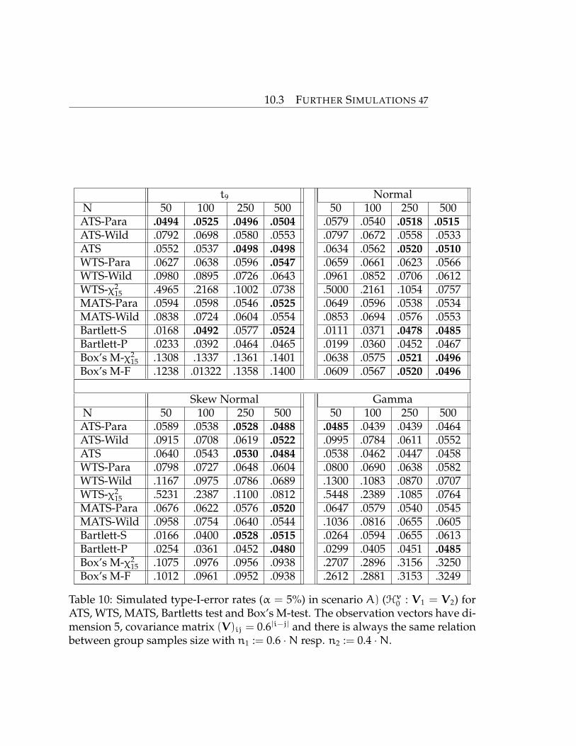
Table 1: Simulated type-I-error rates (α = 5%) in scenario A) (Hv0 : V1 = V2) forATS, WTS, MATS, Bartlett’s test and Box’s M-test, always with the same relationbetween group sample sizes by n1 := 0.6 ·N resp. n2 := 0.4 ·N. The 5-dimensionalobservation vectors have the covariance matrix (V)ij = 0.6|i−j|.

In almost all simulation settings, the wild bootstrap led to more liberal results,

whereas the parametric bootstrap was also liberal for the WTS but had no clear

tendency for the ATS. For larger sample sizes, the ATS with critical values based

on the weighted sum of χ2 random variables behaved similarly to the ATS with

parametric bootstrap, while for smaller sample sizes, the simulated type-I-error

rates differed more from the nominal α-level.

Overall, the results of the ATS were preferable compared to the WTS. This matches

the conventional wisdom that the WTS generally exhibits a liberal behavior and

requires large sample sizes to perform well. Moreover, the WTS requires the con-

dition on the rank of Σ, which is difficult to check in practice because of the special

5.1 Type-I-error


ATS-Para .0465 .0473 .0495 .0505 .0481 .0419 .0454 .0483 .0388 .0363 .0371 .0407ATS-Wild .0682 .0573 .0542 .0527 .0787 .0618 .0550 .0547 .0805 .0645 .0535 .0524ATS .0547 .0501 .0492 .0501 .0566 .0451 .0458 .0487 .0455 .0383 .0373 .0397WTS-Para .0855 .0702 .0622 .0545 .1099 .0886 .0726 .0618 .1441 .1136 .0839 .0711WTS-Wild .1052 .0795 .0660 .0557 .1458 .1112 .0826 .0675 .2099 .1590 .1076 .0847WTS-χ2

4 .1826 .1109 .0682 .0594 .2207 .1277 .0797 .0708 .2609 .1628 .0939 .0761

Table 2: Simulated type-I-error rates (α = 5%) in scenario B) (Hv0 : V111 = ... =V155) for ATS and WTS. The 5-dimensional observation vectors have the covariancematrix (V)ij = 0.6|i−j|.


ATS-Para .0651 .0581 .0537 .0539 .0690 .0589 .0530 .0514 .0715 .0628 .0540 .0552ATS-Wild .0686 .0598 .0542 .0545 .0738 .0621 .0540 .0521 .0848 .0688 .0550 .0556ATS .0739 .0609 .0544 .0541 .0779 .0623 .0540 .0517 .0814 .0655 .0540 .0538WTS-Para .0651 .0581 .0537 .0539 .0690 .0589 .0530 .0514 .0715 .0628 .0540 .0552WTS-Wild .0686 .0598 .0542 .0545 .0738 .0621 .0540 .0521 .0848 .0688 .0550 .0556WTS-χ2

1 .0736 .0605 .0535 .0538 .0775 .0619 .0538 .0518 .0811 .0651 .0540 .0540

Table 3: Simulated type-I-error rates (α = 5%) in scenario C) (Hv0 : tr(V1) = tr(V2))for ATS, WTS, MATS, Bartlett’s test and Box’s M-test, always with the same re-lation between group sample sizes by n1 := 0.6 · N resp. n2 := 0.4 · N. The 5-dimensional observation vectors have the covariance matrix (V)ij = 0.6|i−j|.

structure of Σ. In contrast, the ATS is capable to handle all these scenarios.

Therefore, it remains to compare these tests with those based on Bartlett’s statistic.

The additional condition required for the pooled bootstrap is fulfilled. Therefore,

Table 1 contains also the results of ϕB−P.

For all distributions, ϕ∗ATS showed good results especially for normal distribution

and skewed normal distribution where the type-I-error rate was always better than

those of ϕB−S and ϕB−S. Also for the gamma distribution ϕB−S performed worse

while for bigger N the simulated error-rates of ϕ∗ATS and ϕB−S were comparable.

Most of all ϕ∗ATS provided good values for small samples, while both tests based

on a Bartlett statistic needed large sample sizes. At last, the popular Box’s M-test

worked quite well under normality but showed poor results (type-I-error rates of

5.1 Type-I-error

more than 20%) when this condition was violated. This sensitivity to the violation

of normal distribution may have the consequence in practice that small p-values

could be untrustworthy, independent of whether χ2 or F distribution was used.

But also for normality, the performance was not essentially better than ϕATS and

(with small exceptions) clearly worse than ϕ∗ATS. This also underlines the benefit

of the newly proposed test for this popular null hypothesis.

Moreover, the resampling procedure used in Zhang and Boos (1993) occasionally

encountered covariance matrices without full rank, especially for smaller sample

sizes. This creates issues in the algorithm because the determinant of these matri-

ces is zero, and the logarithm at this point is not defined. Regretfully this situation

wasn’t discussed in the original paper, so we just excluded these values. Certainly,

this would constitute a drastic user intervention in applying the bootstrap and also

influencing the conditional distribution. Nevertheless, it was necessary to use this

adaptation in all our simulations containing these tests. This effect can also occur

in Box’s M-test, but comparatively rarely because there is no bootstrap involved.

All in all, in scenario A) the ATS∗ and the Monte-Carlo ATS test exhibited the

best performance over all distributions and, in particular small sample sizes.

For scenario B) the results in Table 2 again show the good performance of ϕ∗ATS

for small sample sizes. With the exception of the gamma distribution, where for

large sample sizes ϕ?ATS had an error rate closer to our α level, the ATS using the

parametric bootstrap approach had by far the best results.

5.2 Power

At last Table 3 shows the results from scenario C). Due to the fact that the rank

of the hypothesis matrix is 1, there is no difference between the WTS and the ATS.

All our tests ϕ∗ATS,ϕ?ATS and ϕATS showed comparable results while again ϕ∗ATS

had the best small sample performance. In comparison to the other scenarios, the

error rates were a bit worse than before. But we have to take into account that this

is the most challenging hypothesis, which only considers the diagonal elements of

the covariance matrix. Nevertheless, the results for sample sizes 250 and 500 were

convincing.

The effect of using other types of covariance matrices, which is considered in the

supplement, was not significant and not systematic. Therein, we also investi-

gated testing for a given covariance matrix. Here, only the type-I-error rate of

the ANOVA-type statistic with critical values obtained from the parametric boot-

strap and the Monte-Carlo ATS test showed sufficiently good results.

To sum up, we only recommend the use of any of the three tests based on the ATS.

All three exhibited good simulation results for comparably small sample sizes and

are (asymptotically) valid without additional requirements on Σ. Additional sim-

ulations, given in the supplementary material, also confirm this conclusion, espe-

cially for a higher dimension or more groups.

5.2 Power

For a power simulation, it is unfortunately not possible to merely shift the observa-

tions by a proper vector to control the distance from the null hypothesis. Thereto

5.2 Power

we have multiplied the observation vectorsXwith a proper diagonal matrix, given

by ∆ = Id + diag(1, 0, ..., 0) · δ for δ ∈ [0, 3]. This was associated with a one-

point-alternative that is known from testing expectation vectors to be challenging,

namely a deviation in just one component, which is usually difficult to detect.

Figure 1: Simulated power in scenario A) (Hv0 : V1 = V2) for ATS with wild boot-strap, parametric bootstrap, and Monte-Carlo critical values, as well as the testbased on Bartlett’s statistic with separate and pooled bootstrap. The 5-dimensionalvectors were based on the skewed normal distribution, with covariance matrix(V)ij = 0.6|i−j| and n1 = 30,n2 = 20. The considered alternative is a one-point-alternative.

In this way Cvech(∆V∆>

)− ζ 6= 0, were n1 + n2 = 50 was used to investigate

small size behavior, while the dimension was again d = 5, leading to p = 15.

Moreover for a second alternative the observation vectors X were multiplied by

∆ = Id + diag(1, 2, ...,d)/d · δ for δ ∈ [0, 3], which corresponds to a so-called trend-

alternative. Due to computational reasons and because of the performance under

the null hypothesis described in the last section, we have only investigated the

5.2 Power

power of ϕ∗ATS, ϕ?ATS and ϕATS as well as ϕB−P and ϕB−S from Zhang and Boos

(1993) for skewed normal distributed random variables.

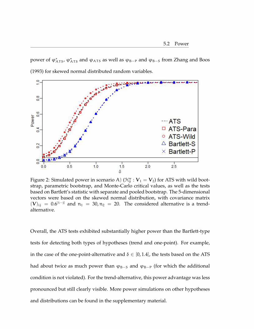
Figure 2: Simulated power in scenario A) (Hv0 : V1 = V2) for ATS with wild boot-strap, parametric bootstrap, and Monte-Carlo critical values, as well as the testsbased on Bartlett’s statistic with separate and pooled bootstrap. The 5-dimensionalvectors were based on the skewed normal distribution, with covariance matrix(V)ij = 0.6|i−j| and n1 = 30,n2 = 20. The considered alternative is a trend-alternative.

Overall, the ATS tests exhibited substantially higher power than the Bartlett-type

tests for detecting both types of hypotheses (trend and one-point). For example,

in the case of the one-point-alternative and δ ∈ [0, 1.4], the tests based on the ATS

had about twice as much power than ϕB−S and ϕB−P (for which the additional

condition is not violated). For the trend-alternative, this power advantage was less

pronounced but still clearly visible. More power simulations on other hypotheses

and distributions can be found in the supplementary material.

6. Review of the required computation time

Besides power and true type-I-error, the computation time is an important criterion

when selecting a proper test. To take account of this, we performed a small sim-

ulation study to compare the computation time for hypothesis A (Hv0 : V1 = V2)

and B (Hv0 : V111 = ... = V1dd). For each hypothesis and quadratic form both boot-

strap techniques were used for 4 different distributions (based on t9-distribution,

Normal-distribution, Skew Normal-distribution and Gamma-distribution) and 2

covariance matrices ((V1)i,j = 0.6|i−j| and V2 = I5 + J5). The average times of 100

such simulation runs are compared. In each run for numerical stability, all of the

eight random vectors were considered, and the time is averaged.

For each test 1.000 bootstrap runs were performed with n1 = 125 observations

resp. n = (150, 100) observations in various dimensions. For the Monte-Carlo-test

again, 10.000 simulation steps were used. The computations were run by means of

the R-computing environment version 3.6.1 R Core Team (2019) on an Intel Xeon

E5430 quad-core CPU running at 2.66 GHz using 16 GB DDR2 memory on a De-

bian GNU Linux 7.8, and the required time in minutes is displayed in Table 4.

Apart from the classical WTS, all versions of the WTS needed clearly more time

than the appropriate ATS. Together with their poor performance in the simula-

tion study, and the additional assumptions on their validity, this makes the WTS

unattractive in comparison. Moreover, for both the ATS and the WTS, there was a

A) B)d 2 5 10 20 2 5 10 20ATS-Para 0.757 5.401 27.928 222.443 0.745 5.332 27.227 195.237ATS-Wild 0.451 0.612 10.831 114.175 0.455 0.599 10.034 87.011ATS 0.086 0.195 0.387 1.231 0.056 0.154 0.276 0.698WTS-Para 0.869 6.625 44.295 462.852 0.839 6.157 34.851 275.909WTS-Wild 0.559 0.916 27.252 355.679 0.545 0.794 17.681 170.063WTS-χ2 0.003 0.004 0.038 0.320 0.003 0.003 0.029 0.133

Table 4: Average computation time in seconds of different test-statistics with dif-ferent dimensions for hypotheses A (Hv0 : V1 = V2) and B (Hv0 : V111 = ... = V1dd).

huge difference in the required computation time between the two bootstrap tech-

niques: For small dimensions, the parametric bootstrap needed about 50 percent

more computation time than the wild bootstrap, while for larger dimensions, it

needed up to more than 20 times longer. This is not surprising because the gener-

ation of normally distributed random vectors is much more time-consuming than

generating random weights. Moreover, the ATS with the Monte-Carlo based crit-

ical values was much faster than all bootstrap approaches as it does not need the

repeated calculation of the estimated covariance matrix of the empirical covari-

ances. Additional results on the computation time for other hypotheses can be

found in the supplementary material.

Recommendation: Together with the simulation results, this makes the ATS with

parametric bootstrap favorable in the situation with smaller dimensions (d 6 5)

due to its accurate type-I-error control. For larger dimensions (d > 10), however,

we recommend its Monte-Carlo implementation due to the much faster computa-

tion time.

6.1 SELECTION OF PROPER HYPOTHESIS MATRIX C


As mentioned at the beginning, considering a general ζ 6= 0p as well as general,

not necessarily idempotent and symmetric matrices C for the description of the

hypothesis is favorable. Beyond more freedom of choosing proper matrices, the

major advantage consists of different computational times. Indeed, depending on

the hypothesis of interest, it is possible to choose matricesC ∈ Rm×ap withm con-

siderably smaller than ap. We exemplify this issue for the following hypotheses:

A) Equal Covariance Matrices: Testing the hypothesis Hv0 : {V1 = V2} = {C(A)v =

0} is usually described by C(A) = P2 ⊗ Ip. However, the choice C̃(A) =

(1,−1)⊗ Ip ∈ Rp×2p is computationally more efficient.

B) Equal Diagonal Elements: The hypothesis Hv0 : {V111 = ... = V1dd} =

{C(B)v = 0} can, e.g., be described by C(B) = diag(hd) − hd · h>d/d. In con-

trast, the equivalent description by C̃(B) = (1d−1, 0(d−1)×(d−1),−e1, 0(d−1)×(d−2),

−e2, ..., 0d−1,ed−1) ∈ R(d−1)×p saves a considerable amount of time. Here, ej

denotes the d− 1 dimensional vector containing 1 in the j-th component and

0 elsewhere.

C) Equal traces: Testing Hv0 : {tr(V1) = tr(V2)} = {C(C)v = 0} is usually de-

scribed by C(C) = P2 ⊗ [hd · h>d ]/d. An equivalent expression is achieved

with the smaller matrix C̃(C) = (1,−1)⊗ hd/d ∈ R1×2p.

D) Test for a given trace: Hv0 : {tr(V1) = γ} = {C(D)v = hd · γ} for a given value


γ ∈ R can either be described by C̃(D) = h>d/d ∈ R1×p orC(D) = [hd ·h>d ]/d,

where the first choice has considerably less rows.

For these four examples, we performed a small simulation study to compare the

computational efficiency of the smaller matrix C̃with respect to the quadratic ma-

trix C: To get reliable results, the same setting as before was used, and the results

are displayed in Table 5 and Table 6. Depending on the dimension, statistic, and

hypothesis of interest, the time savings ranged from less than 1% to more than

99%. In fact, for most methods, the savings increased with increasing dimension.

Only for the Monte-Carlo ATS test, some fluctuations were visible.

d A) ATS-Para A) ATS A) WTS-Para C) ATS-Para C) ATS C) WTS-Para2 0.9842 0.6516 0.9660 0.9780 0.4299 0.95835 0.9872 0.7904 0.9294 0.9713 0.2050 0.9257

10 0.9749 0.7130 0.7868 0.9553 0.1129 0.689320 0.8777 0.5669 0.5961 0.8020 0.0966 0.4300

Table 5: Computation time for non quadratic hypothesis matrices C̃ relative to pro-jection matricesC. Different test-statistics, hypotheses, and dimensions are consid-ered.

d B) ATS-Para B) ATS B) WTS-Para D) ATS-Para D) ATS D) WTS-Para2 0.8484 0.5650 0.8493 0.8523 0.5668 0.84655 0.1623 0.3811 0.1626 0.1392 0.1888 0.1462

10 0.1014 0.4316 0.0917 0.0336 0.1140 0.031620 0.0439 0.2719 0.0372 0.0052 0.0540 0.0040

Table 6: Computation time for non quadratic hypothesis matrices C̃ relative to pro-jection matricesC. Different test-statistics, hypotheses, and dimensions are consid-ered.

Moreover, a clear impact of the number of groups could be seen. The reason for

this is that for D), the reduction of the dimension can be implemented before the

calculation of covariance matrices or similar steps. The latter steps benefitted con-

siderably from this reduction leading to significantly lower computation time.

The exact time measurements for all four hypotheses and both kinds of matrices

can be found in the supplementary material.

7. ILLUSTRATIVE DATA ANALYSIS

To demonstrate the use of the proposed methods, we have re-analyzed neurolog-

ical data on cognitive impairments. In Bathke et al. (2018) the question was ex-

amined whether EEG- or SPECT-features were preferable to differentiate between

three different diagnoses of impairments - subjective cognitive complaints (SCC),

mild cognitive impairment (MCI), and Alzheimer disease (AD). The correspond-

ing trial was conducted at the University Clinic of Salzburg, Department of Neu-

rology. Here one hundred sixty patients were diagnosed with either AD, MCI, or

SCC, based on neuropsychological diagnostics, as well as a neurological examina-

tion. This data set has been included in the R-package manova.rm by Friedrich et al.

(2019). The following Table 7 contains the number of patients divided by sex and

diagnosis.

AD MCI SCCmale 12 27 20female 24 30 47

Table 7: Number of observations for the different factor level combinations of sexand diagnosis.

For each patient, d = 6 different kinds of EEG variables were investigated, which

leads to p = 21 variance and covariance parameters. As the male AD and SCC

group only contain 12 and 20 observations, respectively, an application of the WTS

would not be possible.

In Bathke et al. (2018), the authors descriptively checked the empirical covariances

matrices to judge that the assumption of equal covariance matrices between the

different groups is unlikely. However, this presumption has not been inferred sta-

tistically. To close this gap, we first test the null hypothesis of equal covariance

matrices between the six different groups using the newly proposed methods. Ap-

plying the ATS with parametric resp. wild bootstrap led to p-values of 0.0275 and

0.0008.

In comparison, the Bartlett-S test of Zhang and Boos (1993) led to a p-value of

0.3484, potentially reflecting its bad power observed in Section 5 and also by the

authors. Moreover, their Bartlett-P test for the smaller null hypothesis (addition-

ally postulating equality of vectorized moments) shows a small p-value of 0.00019998.

As a next step, we take the underlying factorial structure of the data into account

and test, for illustrational purposes, the following hypotheses:

a) Homogeneity of covariance matrices between different diagnoses,

b) Homogeneity of covariance matrices between different sexes,

c) Equality of total variance between different diagnosis groups,

d) Equality of total variance between different sexes.

For the first two hypotheses, we calculated the ATS with wild and parametric boot-

strap as well as Bartlett’s test statistic with separate and pooled bootstrap. Consid-

ering the trace hypotheses, just the first two tests are applicable, and in all cases,

the one-sided tests are used based on 10.000 bootstrap runs. The results are pre-

sented in Table 8 and Table 9.

ATS-Para ATS-Wild Bartlett-S Bartlett-Pp-value p-value p-value p-value

Ha0 : male AD vs. MCI 0.1000 0.0282 0.1742 0.0184

Ha0 : male AD vs. SCC <0.0001 <0.0001 0.0545 0.0634

Ha0 : male MCI vs. SCC 0.8767 0.9801 0.1383 0.0078

Ha0 : female AD vs. MCI 0.0613 0.0559 0.1050 0.1480

Ha0 : female AD vs. SCC 0.0128 0.0095 0.0138 0.0183

Ha0 : female MCI vs. SCC 0.5656 0.6004 0.8964 0.8988

Hb0 : AD male vs. female 0.1008 0.0279 0.2479 0.0542

Hb0 : MCI male vs. female 0.2455 0.2417 0.3695 0.4003

Hb0 : SCC male vs. female 0.2066 0.1914 0.2656 0.1648

Table 8: P-values of ATS with wild resp. parametric bootstrap and Bartlett’s teststatistic with separate resp. pooled bootstrap for testing equality of covariancematrices.

ATS-Para ATS-Wildp-value p-value

Hc0 : male AD vs. MCI 0.0733 0.0635

Hc0 : male AD vs. SCC <0.0001 <0.0001

Hc0 : male MCI vs. SCC 0.6146 0.6297

Hc0 : female AD vs. MCI 0.0074 0.0091

Hc0 : female AD vs. SCC 0.0006 0.0012

Hc0 : female MCI vs. SCC 0.3687 0.3811

Hd0 : AD male vs. female 0.0881 0.0834

Hd0 : MCI male vs. female 0.1582 0.1592

Hd0 : SCC male vs. female 0.3423 0.3744

Table 9: P-values of ATS with wild resp. parametric bootstrap for testing equalityof traces containing covariance matrices.

It is noticeable that both tests based on the ATS clearly reject the null hypothesis of

equal covariances for AD and SCC for both sexes at level 5%, while the p-values of

both Bartlett’s tests are not significant. An explanation for this combination with

fewer samples may be given by the good small sample performance of the ATS

observed in Section 5 and the quite low power of Bartlett’s test statistic, which

was already mentioned in Zhang and Boos (1993). Moreover, the only cases where

both Bartlett’s test-statistics have smaller p- values are for the combination with

the largest sample sizes. Unfortunately, the separate bootstrap has again really low

power, while it is questionable whether the additional condition for pooled boot-

strap is fulfilled. For the user, this condition is almost as hard to check as equality

of covariance. This could lead to the almost circular situation where another test

would be necessary to allow for the pooled bootstrap approach for testing homo-

geneity of covariances.

The null hypothesis of equal total covariance resp. equal traces could be rejected

significantly (at level 5%) by both bootstrap tests in three cases. Perhaps surprising

at first is that the null hypothesis of equal covariance matrices between the female

AD and MCI groups could not be rejected, but the joint univariate null hypothesis

of equal traces could now be rejected at level 5%.

Although the hypothesis of equal covariance matrices couldn’t be rejected in each

case, it shows that sex and diagnosis are likely to have an effect on the covari-

ance matrix. This illustrative analysis underpins that the approach of Bathke et al.

(2018), which can deal with covariance heterogeneity, was very reasonable.

8. CONCLUSION & OUTLOOK

In the present paper, we have introduced and evaluated a unified approach to test-

ing a variety of quite general null hypotheses formulated in terms of covariance

matrices. The proposed method is valid under a comparatively small number of

requirements that are verifiable in practice. Previously existing procedures for the

situation addressed here had suffered from low power to detect alternatives, were

limited to only a few specific null hypotheses, or needed various requirements in

particular regarding the data generating distribution.

Under weak conditions, we have proved the asymptotic normality of the differ-

ence between the vectorized covariance matrices and their corresponding vector-

ized empirical versions. We considered two-test statistics, which are based upon

the vectorized empirical covariance matrix and an estimator of its own covariance:

a Wald-type-statistic (WTS) as well as an ANOVA-type-statistic (ATS). These ex-

hibit the usual advantages and disadvantages that are already well-known from

the literature on mean-based inference. In order to take care of some of these diffi-

culties, namely the critical value for the ATS being unknown and the WTS requir-

ing a rather large sample size, two kinds of bootstrap were used. On this occasion,

specific adaptions were needed to take account of the special situation where in-

ference is not on the expectation vectors but on the covariance matrices.

To investigate the properties of the newly constructed tests, an extensive simula-

tion study was done. For this purpose, several different hypotheses were consid-

ered, and the type-I-error control, as well as the power to detect deviations from

the null hypothesis, were compared to existing test procedures. The ATS showed a

quite accurate error control in each of the hypotheses, in particular in comparison

with competing procedures. Note that for most hypotheses, no appropriate com-

peting test is available. The simulated power of the proposed tests was fine, even

for moderately small sample sizes (n1 = 30,n2 = 20). This is a major advantage

when comparing with existing procedures for testing homogeneity of covariances,

even considering that they usually require further assumptions .

In future research, we would like to investigate in more detail the large number

of possible null hypotheses that are included in our model as special cases. For

example, tests for given covariance structures (such as compound symmetry or

autoregressive) with unknown parameters are of great interest. Moreover, our re-

sults allow for a variety of new tests for hypotheses that can be derived from our

model, for example, testing the equality of determinants of covariances matrices.

The model and the assumption of finite fourth moments exclude some distribu-

tions like, for example, heavy-tailed distributions. For such distributions, probably

a similar approach can be developed using scatter matrices.

Finally, it is still unclear whether our approach can be extended to high-dimensional

settings. There already exist some inspiring solutions, see for example, Chi et al.

(2012), Li and Chen (2012), Li and Qin (2014)), and Cai et al. (2013). However, they

are only constructed for special situations and do not allow the same flexibility

36

as our approach. Due to different technical approaches, this task remains future

research. Furthermore, we are planning to investigate extensions of our work by

combining it with results on high-dimensional covariance matrix estimators, as

considered in Cai et al. (2016).

9. ACKNOWLEDGMENT

Paavo Sattler and Markus Pauly would like to thank the German Research Founda-

tion for the support received within project PA 2409/4-1. Moreover, Arne Bathke

expresses his thanks to the Austrian Science Fund (FWF) for the funding received

through project I 2697-N31.

10. Appendix

10.1 The Model

The considered semiparametric model can be shortly defined through Xik = µi +

εik, while εik are i.i.d. d-dimensional random vectors with E(εik) = 0d and

Var(εik) = Vi > 0. For εik, which is called the non-parametric part, it is allowed

that each component are from a completly different distribution. We additionaly

assume finite fourth moments for all components through E(||εik||4) < ∞. The

number of groups a can persist from multiple crossed factors, where for one, two

10.2 Proofs 37

and three factors the model is given through:

Xik = µi + εik

= µ+ αi + βj + (αβ)ij + εijk

= µ+ αi + βj + γ` + (αβ)ij + (βγ)j` + (αγ)i` + (αβγ)ij` + εij`k,

with i = 1, ...,a , j = 1, ..., J , ` = 1, ....,L and k = 1, ...,K. In this case it holds

a = J · L · K, and each group represents one combination of these three factors.

Like this, the dimension can also consist of multiple factors, for example, in re-

peated measure design, where often the factors time and treatment are crossed.

Then the dimension is divided into smaller parts, one for each factor-combination.

10.2 Proofs

The asymptotic distribution, discussed in Theorem 1 is well known (for example,

from Browne and Shapiro (1986)), but based on the importance of the techniques

presented in this paper, we will prove it shortly. Moreover, this allows getting the

idea of our bootstrap approaches later on.

Proof of Theorem 1: First we consider the difference between the vector vi and its

estimated version v̂i, multiplied with√N

√N(v̂i − vi)

=√Nvech

(1

ni−1

ni∑k=1

[εikε

>ik −Vi

]+ 1ni−1Vi −

1ni−1(

√ni εi·)(

√ni εi·)

>)

.

10.2 Proofs 38

Due to Slutzky and the multivariate Central limit theorem, the second and third

term tends to zero in probability. Thus, it is sufficient to consider the first term. But

this converges to Nd(0d, κ−1i Σi) in distribution again by the multivariate central

limit theorem, which gives us the result due to independence of the groups.

This convergence would also follow from Zhang and Boos (1993), but the bootstrap

approach is based on this proof, so it is helpful to outline it again. To use this result,

a consistent estimator for the covariance matrix Σ is needed.

Consistency of Σ̂: Because vech(εikε>ik) are i.i.d. vectors, we know that

Σ̃i =

ni∑k=1

[vech(εikε>ik) −

ni∑̀=1

vech(εi`ε>i`)ni

] [vech(εikε>ik) −

ni∑̀=1

vech(εi`ε>i`)ni

]>ni − 1

is a consistent estimator for Σi. However, we can not calculate this estimator, since

Cov(εi) = Cov(Xi), but in general Cov(vech(εiε>i )) 6= Cov(vech(XiX>i )) and µi

is unknown. So we use centered vectors X̃ik to formulate the proper covariance

matrix Σ̂i. These vectors are not independent, so we prove the consistency of our

estimator through that Σ̂i − Σ̃i converge almost sure to 0. This is done by

10.2 Proofs 39

Σ̂i − Σ̃i

= 4nini−1

(vech(Xiµ>i )vech(Xiµ>i )

> − vech(XiX>i )vech(XiX

>i )>)

+ 4ni−1

∑nik=1

[vech(XikX

>i )vech(XikX

>i )> − vech(Xikµ>i )vech(Xikµ>i )

>]

+ 4ni−1

∑nik=1

[vech(XikX>ik)vech(Xiµ>i )

> − vech(XikX>ik)vech(XiX>i )>]

+ 4ni−1

∑nik=1

[vech(XikX>ik)vech(Xikµ>i )

> − vech(XikX>ik)vech(XikX>i )>]

= 4nini−1

(vech(Xi(µi − Xi)>)vech(Xiµ>i + XiX

>i )>)

+ 4ni−1

∑nik=1

[vech(Xik(Xi − µi)>)vech(Xik(Xi − µi)> + 2Xikµ>i )

>]+ 4

ni−1

∑nik=1

[vech(XikX>ik)vech(Xi(µi − Xi)>)>

]+ 4

ni−1

∑nik=1

[vech(XikX>ik)vech(Xik(µi − Xi)>)>

].

It is enough to show that each component of this difference converges almost sure

to zero. So with |X| denoting the absolute value of each component we get for ar-

bitrary h, j ∈ {1, ...,p} that

|(Σ̂i − Σ̃i)h,j|

6 4nini−1 |vech(Xi(µi − Xi)>)h|·|vech(Xiµ>i + XiX

>i )j|

+ 4ni−1

∑nik=1|vech(Xik(Xi − µi)>)h|·|vech(Xik(Xi − µi)> + 2Xikµ>i )j|

+ 4ni−1

∑nik=1|vech(XikX>ik)j|·|vech(Xi(µi − Xi)>)h|

+ 4ni−1

∑nik=1|vech(XikX>ik)j|·|vech(Xik(µi − Xi)>)h|

10.2 Proofs 41

prooved.

Proof of Theorem 2: All results are known (see, e.g., ?), but sometimes only idem-

potent symmetric hypothesis matrices are considered, so we will repeat them for

general matrices C. From Theorem 1 it follows that all these quadratic forms can

be written as the sum of a quadratic form with normal distributed random vectors

and vectors which converge in distribution to zero.

Therefore with Z ∼ Na·p (0a·p, Iap) and√N(v̂− v)

D−→ Σ1/2Z we get

Q̂v = N [Cv̂− ζ]>E(C, Σ̂) [Cv̂− ζ]

H0= N · (v̂− v)>C>E(C, Σ̂)C(v̂− v)

D→(Σ1/2Z

)>C>E(C, Σ̂)C

(Σ1/2Z

)= Z>Σ1/2C>E(C, Σ̂)CΣ1/2Z

D=

∑a·p`=1 λ`B`,

with λ`, ` = 1, ...,ap eigenvalues of(Σ1/2C>E(C,Σ)CΣ1/2) and B`i.i.d.∼ χ2

1. Note,

that we have used that (Σ1/2C>E(C,Σ)CΣ1/2) is symmetric and therefore has a

spectral representation. The rest of the proof follows from the fact that the mul-

tivariate standard normal distribution is invariant under orthogonal transforma-

tions, the consistency of E(C, Σ̂) for E(C,Σ) and the continuous mapping theo-

rem.

Proof of Theorem 3: It is sufficient to prove the part for the single groups because

the second part is just the combination of all groups.

10.2 Proofs 42

This result follows from a part-wise application (given the data) of the multivariate

Lindeberg-Feller-Theorem. So it remains to show that all conditions are fulfilled,

for which we use the fact that Y∗ underX is p dimensional normal distributed with

expectation 0p and variance Σ̂i:

1.)=ni∑k=1

E(√

NniY∗ik

∣∣∣X) =ni∑k=1

√Nni· E(Y∗ik

∣∣∣X) = 0

2.)=ni∑k=1

Cov(√

NniY∗ik

∣∣∣X) =ni∑k=1

Nn2i

Σ̂iP→ 1κiΣi

3). limN→∞

ni∑k=1

E(∣∣∣∣∣∣√Nni Y∗ik∣∣∣∣∣∣2 · 11∣∣∣∣√N

niY∗ik

∣∣∣∣>δ ∣∣∣X)

= limN→∞ N

n2i

ni∑k=1

E(∣∣∣∣Y∗i1∣∣∣∣2 · 11||Y∗i1||>δ

ni√N

∣∣∣X)= 1

κi· limN→∞E

(∣∣∣∣Y∗i1∣∣∣∣2 · 11||Y∗i1||>δni√N

∣∣∣X)6 1

κi· limN→∞

√E (||Y∗i1||

2 |X) ·√E(

11||Y∗i1||>δni√N

∣∣∣X) = 0

Here we used the Cauchy-Bunjakowski-Schwarz-Inequality and that we know

E(∣∣∣∣Y∗i1∣∣∣∣2 ∣∣X). Moreover because of the condition ni/N → κi and as a conse-

quence δ · ni/√N → ∞ it holds P

(∣∣∣∣Y∗i1∣∣∣∣ > δ · ni/√N) → 0, which leads to the

result.

Therefore, given the data X it follows that√N · Y∗i converges in distribution to

Np (0p, 1/κi · Σi) and due to indepence also√N · Y∗ converges in distribution to

10.2 Proofs 43

Na·p (0a·p,⊕ai=1 1/κi · Σi). As the empirical covariance matrix of the bootstrap

sample is also consistent, with Σ̂∗i

P→ Σ̂i the result follows from Consistency of

Σ̂i and the triangle inequality. Moreover, Σ̂∗ P→ Σ follows by continuous mapping

theorem.

Proof of Theorem 4: Again we have to show the conditions of the Lindeberg-Feller

theorem part-wise, given the data X = (X>11, . . . ,X>ana)> :

1.)=ni∑k=1

E(√

NniY?ik

∣∣∣X) =ni∑k=1

√Nni

E(Wik) ·[

vech(X̃ikX̃>ik) −

ni∑i=1

vech(X̃ikX̃>ik)

ni

]= 0

2.)ni∑k=1

Cov(√

NniY?ik

∣∣∣X) = Nn2i

E(W2i1

)· (ni − 1) · Σ̂i

= ni−1ni

NniΣ̂i

P→ 1κiΣi

For the last part we use that given the data∣∣∣∣Y?

i1

∣∣∣∣2 · 11||Y?i1||>δ

ni√N

6∣∣∣∣Y?

i1

∣∣∣∣2 has a

finite expectation value. Moreover Lebesgue’s dominated convergence theorem

with ni/√N→∞ and P

(∣∣∣∣Y?i1

∣∣∣∣ > δ · ni/√N)→ 0, leads to the result.

3). limni→∞

ni∑k=1

E(∣∣∣∣∣∣√Nni Y?

ik

∣∣∣∣∣∣2 · 11∣∣∣∣√NniY?ik

∣∣∣∣>δ ∣∣∣X)

= limN→∞ N

(ni)2

ni∑k=1

E(∣∣∣∣Y?

i1

∣∣∣∣2 · 11||Y?i1||>δ

ni√N

∣∣∣X)= 1

κi· limN→∞E

(∣∣∣∣Y?i1

∣∣∣∣2 · 11||Y?i1||>δ

ni√N

∣∣∣X)= 1

κi· E(

limN→∞

∣∣∣∣Y?i1

∣∣∣∣2 · 11||Y?i1||>δ

ni√N

∣∣∣X) = 0

10.2 Proofs 44

Hence, given the data we have convergence in distribution of√N ·Y?

i and√N ·Y?

to Np (0p, 1/κi · Σi) resp. Na·p (0a·p,⊕ai=1 1/κi · Σi).

The consistency of the covariance estimator is proven analogous to the parametric

bootstrap.

Proof of Corollary 1 and Corollary 2 : As in Theorem 2 it holds that

N [Cv̂− ζ]>E(C,Σ) [Cv̂− ζ] D−→

a·p∑`=1

λ`B`,

where λ`, ` = 1, ...,ap are the eigenvalues of (Σ1/2C>E(C,Σ)CΣ1/2) and B`i.i.d.∼ χ2

1.

Moreover, similar to Theorem 4 it follows that given the data,

N[CY∗]>E(C, Σ̂

∗)[C Y

∗]

D→a·p∑`=1

λ`B`

and

N[CY

?]>E(C, Σ̂

?)[C Y

?]

D→a·p∑`=1

λ`B`,

because Σ̂∗

and Σ̂?

are consistent estimators for Σ.

The result especially allows the application of the parametric bootstrap version of

the MATS given by

MATS∗ := N[CY∗]> (

CΣ̂∗0C>)+ [

CY∗]

(10.7)

10.3 FURTHER SIMULATIONS 45

and the wild bootstrap version given by

MATS? := N[CY

?]> (

CΣ̂?

0C>)+ [

CY?]

. (10.8)

10.3 FURTHER SIMULATIONS

In this section, we expand the simulations from Section 5, for example, through

more null hypotheses and bootstrap versions of the MATS statistic defined in (10.7)

and (10.8). To investigate the influence of the covariance matrix, for the distribu-

tional setting an additional covariance matrix V2 is used, which is a compound

symmetry matrix given by V2 := I5 + J5. The same distributions as in Section 5

were used for the error term, but we also simulated one more, which is based on a

standardized centered t-distribution with 9 degrees of freedom.

Testing for the equality of covariances is an important hypothesis that usually be-

comes more demanding for an increasing number of groups. Therefore, for all the

random vectors, we investigated an additional scenario:

E) a = 3 Hv0 : V1 = V2 = V3,

where also scenario E) can be formulated with an idempotent symmetric matrix

C(E) = P3⊗I15. For scenarioA) and C) we considered n1 = 0.6 ·N and n2 = 0.4 ·N

with N = (50, 100, 250, 500) and for B) n1 = (25, 50, 125, 250). In case of the three

groups we considered n1 := 0.4 · N, n2 := 0.25 · N and n3 := 0.35 · N for N from


80 up to 800. This choice makes the sample sizes similar to the situation with two

groups and therefore increases the comparability.

We should keep in mind that in this case, p is 15, which makes some of these

sample sizes small in relation to the dimension. The WTS resp. MATS are part of

our simulation, although in practice it is quite difficult or even impossible to check

the necessary conditions Σ > 0 resp. Σ0 > 0.

Again it could be seen in all tables that the wild bootstrap lead to more liberal re-

sults and the parametric bootstrap had less liberal or even conservative test results.

This hold for all our quadratic forms, the ATS, the WTS, and the MATS. Overall hy-

potheses and settings, the MATS-test-statistic seems to perform between the ATS

and the WTS but was still preferable over the Bartlett test-statistics in scenario A).

For the additional covariance matrix, again the ATS with parametric bootstrap had

the best type-I-error control in nearly every setting. Moreover, the influence of the

used covariance matrix could be seen, but it neither seemed to be strong nor had a

systematical effect on the quality. For the additional distribution ϕ∗ATS exhibited a

good performance in most cases, particularly for scenario A). So Table 10-Table 13

in total confirmed the results from Section 5. The usage and the performance of

the MATS showed the variety of our approach one more time.

As expected, it can be seen in Table 16 and Table 17 that all tests performed gener-

ally worse than for just two groups, although some individual results were better.

In particular, for both Barlett tests and all WTS tests, there was a significant wors-

ening. In part, the error rate was almost halved for the Bartlett tests and doubled


t9 NormalN 50 100 250 500 50 100 250 500ATS-Para .0494 .0525 .0496 .0504 .0579 .0540 .0518 .0515ATS-Wild .0792 .0698 .0580 .0553 .0797 .0672 .0558 .0533ATS .0552 .0537 .0498 .0498 .0634 .0562 .0520 .0510WTS-Para .0627 .0638 .0596 .0547 .0659 .0661 .0623 .0566WTS-Wild .0980 .0895 .0726 .0643 .0961 .0852 .0706 .0612WTS-χ2

15 .4965 .2168 .1002 .0738 .5000 .2161 .1054 .0757MATS-Para .0594 .0598 .0546 .0525 .0649 .0596 .0538 .0534MATS-Wild .0838 .0724 .0604 .0554 .0853 .0694 .0576 .0553Bartlett-S .0168 .0492 .0577 .0524 .0111 .0371 .0478 .0485Bartlett-P .0233 .0392 .0464 .0465 .0199 .0360 .0452 .0467Box’s M-χ2

15 .1308 .1337 .1361 .1401 .0638 .0575 .0521 .0496Box’s M-F .1238 .01322 .1358 .1400 .0609 .0567 .0520 .0496

Skew Normal GammaN 50 100 250 500 50 100 250 500ATS-Para .0589 .0538 .0528 .0488 .0485 .0439 .0439 .0464ATS-Wild .0915 .0708 .0619 .0522 .0995 .0784 .0611 .0552ATS .0640 .0543 .0530 .0484 .0538 .0462 .0447 .0458WTS-Para .0798 .0727 .0648 .0604 .0800 .0690 .0638 .0582WTS-Wild .1167 .0975 .0786 .0689 .1300 .1083 .0870 .0707WTS-χ2


15 .1075 .0976 .0956 .0938 .2707 .2896 .3156 .3250Box’s M-F .1012 .0961 .0952 .0938 .2612 .2881 .3153 .3249

Table 10: Simulated type-I-error rates (α = 5%) in scenario A) (Hv0 : V1 = V2) forATS, WTS, MATS, Bartletts test and Box’s M-test. The observation vectors have di-mension 5, covariance matrix (V)ij = 0.6|i−j| and there is always the same relationbetween group samples size with n1 := 0.6 ·N resp. n2 := 0.4 ·N.




15 .1308 .1337 .1361 .1401 .0638 .0575 .0521 .0496Box’s M-F .1238 .1322 .1358 .1400 .0609 .0567 .0520 .0496



15 .1075 .0976 .0956 .0938 .2707 .2896 .3156 .3250Box’s M-F .1012 .0961 .0952 .0938 .2612 .2881 .3153 .3249

Table 11: Simulated type-I-error rates (α = 5%) in scenario A) (Hv0 : V1 = V2) forATS, WTS, MATS, Bartletts test and Box’s M-test. The observation vectors havedimension 5, covariance matrix V = I5 + J5 and there is always the same relationbetween group samples size with n1 := 0.6 ·N resp. n2 := 0.4 ·N.


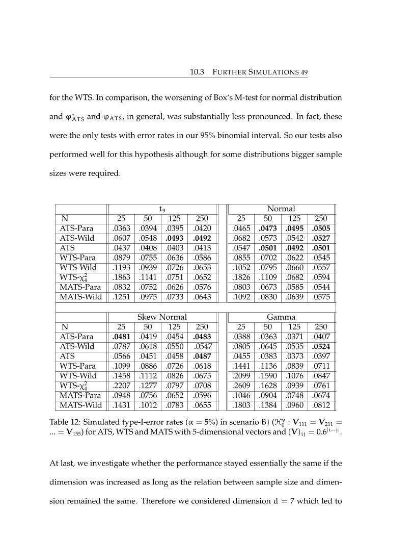
for the WTS. In comparison, the worsening of Box‘s M-test for normal distribution

and ϕ∗ATS and ϕATS, in general, was substantially less pronounced. In fact, these

were the only tests with error rates in our 95% binomial interval. So our tests also

performed well for this hypothesis although for some distributions bigger sample

sizes were required.


4 .1863 .1141 .0751 .0652 .1826 .1109 .0682 .0594MATS-Para .0832 .0752 .0626 .0576 .0803 .0673 .0585 .0544MATS-Wild .1251 .0975 .0733 .0643 .1092 .0830 .0639 .0575



Table 12: Simulated type-I-error rates (α = 5%) in scenario B) (Hv0 : V111 = V211 =... = V155) for ATS, WTS and MATS with 5-dimensional vectors and (V)ij = 0.6|i−j|.

At last, we investigate whether the performance stayed essentially the same if the

dimension was increased as long as the relation between sample size and dimen-

sion remained the same. Therefore we considered dimension d = 7 which led to






Table 13: Simulated type-I-error rates (α = 5%) in scenario B) (Hv0 : V111 = V122 =... = V155) for ATS, WTS and MATS with 5-dimensional vectors and V = I5 + J5.






Table 14: Simulated type-I-error rates (α = 5%) in scenario C) (Hv0 : tr(V1) =tr(V2)) for ATS, WTS, and MATS. The observation vectors have dimension 5, co-variance matrix (V)ij = 0.6|i−j| and there is always the same relation betweengroup samples size with n1 := 0.6 ·N resp. n2 := 0.4 ·N.






Table 15: Simulated type-I-error rates (α = 5%) in scenario C) (Hv0 : tr(V1) =tr(V2)) for ATS, WTS, and MATS. The observation vectors have dimension 5, co-variance matrix V = I5 + J5 and there is always the same relation between groupsamples size with n1 := 0.6 ·N resp. n2 := 0.4 ·N.




30 .1580 .1678 .1825 .1872 .0671 .0560 .0497 .0517Box’s M-F .1521 .1653 .1824 .1872 .0638 .0546 .0496 .0517



30 .1211 .1156 .1138 .1160 .3819 .4306 .4661 .4776Box’s M-F .1148 .1139 .1136 .1159 .3723 .4281 .4657 .4775

Table 16: Simulated type-I-error rates (α = 5%) in scenario E) (Hv0 : V1 = V2 = V3)for ATS, WTS, and MATS. The observation vectors have dimension 5, covariancematrix (V)ij = 0.6|i−j| and there is always the same relation between group sam-ples size with n1 := 0.4 ·N, n2 := 0.25 ·N and n3 := 0.35 ·N.




30 .1580 .1678 .1825 .1872 .0671 .0560 .0497 .0517Box’s M-F .1521 .1653 .1824 .1872 .0638 .0546 .0496 .0517



30 .1211 .1156 .1138 .1160 .3819 .4306 .4661 .4776Box’s M-F .1148 .1139 .1136 .1159 .3723 .4281 .4657 .4775

Table 17: Simulated type-I-error rates (α = 5%) in scenario E) (Hv0 : V1 = V2 = V3)for ATS, WTS, and MATS. The observation vectors have dimension 5, covariancematrix (V) = I5 + J5 and there is always the same relation between group samplessize with n1 := 0.4 ·N, n2 := 0.25 ·N and n3 := 0.35 ·N.


p = 28. Note that this is substantially larger than for d = 5 where we had p = 15.

With N = (70, 140, 350, 700) we considered the setting from A) (Hv0 : V1 = V2)

with the same kind of distributions and covariance matrices, but for dimension 7.

The corresponding results are displayed in Table 18 and Table 19.

It is interesting, that the higher dimension together with the larger number of ob-

servations improved the results of our test for some distributions like for the skew

normal distribution, while for others the performance deteriorated, e.g., for the

gamma distribution. But across all distributions, the quality of the tests’ perfor-

mance was comparable to the situation with dimension 5. In some way, this is

surprising because the sample size was increased in linear relation to the dimen-

sion d, and not in relation to the dimension of the vectorized covariance matrix

p, where the latter grows much more rapidly. Considering the dimension of this

vector as the decisive factor, the relative sample sizes are clearly lower than for di-

mension 5. Once more, this simulation demonstrated good small sample behavior.

By contrast, the results of both Bartlett statistics showed the impact of this smaller

sample size in relation to p. In particular, for N = 70 and N = 140, a worse type-I-

error control could be seen, for example, for the skewed normal distribution with

autoregressive covariance matrix. Moreover, Box’s M test with both kinds of criti-

cal values performed considerably worse in the case of normally distributed data.

While for larger sample sizes in the case of dimension 5 all error rates were in the

95% binomial interval, for dimension 7 none of them was in the interval.

10.4 More Power Plots56

The results from this setting show that in cases of higher dimension, the perfor-

mance for smaller sample sizes is of essential importance. Unfortunately, most of

the existing procedures do not perform in a satisfactory way in this situation.

To sum up,ϕ∗ATS andϕATS led to good finite sample results, even for small sample

sizes and challenging null hypotheses or higher dimension. The excellent small

sample approximation and the variety of applicable situations for this approach

make the results for the ATS with parametric bootstrap even a little bit more con-

vincing. The tests from Zhang and Boos (1993) were inadequate in most of the

cases. Also, neither the WTS nor the MATS based tests were reliable choices for

small to moderate sample size settings.

In comparison, the ATS with parametric bootstrap as well as based on a Monte-

Carlo simulation exhibited rather good results in particular for higher dimension.

Moreover, for more groups, these tests were the only ones with a sufficiently con-

vincing performance in case of non-normality. Thus, these additional simulations

emphasized again the wide applicability of both of these newly developed tests.

10.4 More Power Plots

For the power simulation, we again considered, on the one hand, ϕ∗ATS, ϕ?ATS and

ϕATS, and on the other hand,ϕB−S andϕB−P, all with small (N = 25 resp. N = 50)

as well as moderate(N=50 resp. N=100) sample size. The results from Section

5 showed that the one-point-alternative is of greater interest, so we just consid-




28 .1440 .1396 .1448 .1442 .0719 .0618 .0562 .0539Box’s M-F .1353 .1374 .1445 .1441 .0654 .0608 .0561 .0539



28 .1123 .1027 .0926 .0939 .3046 .3241 .3417 .3557Box’s M-F .1045 .1012 .0924 .0939 .2933 .3204 .3413 .3555

Table 18: Simulated type-I-error rates (α = 5%) in scenario A) (Hv0 : V1 = V2) forATS, WTS, and MATS. The observation vectors have dimension 7, covariance ma-trix (V)ij = 0.6|i−j| and there is always the same relation between group samplessize with n1 := 0.6 ·N, resp. n2 := 0.4 ·N.




28 .1440 .1396 .1448 .1442 .0719 .0618 .0562 .0539Box’s M-F .1353 .1374 .1445 .1441 .0654 .0608 .0561 .0539



28 .1123 .1027 .0926 .0939 .3046 .3241 .3417 .3557Box’s M-F .1045 .1012 .0924 .0939 .2933 .3204 .3413 .3555

Table 19: Simulated type-I-error rates (α = 5%) in scenario A) (Hv0 : V1 = V2)for ATS, WTS, and MATS. The observation vectors have dimension 7, covariancematrix (V) = I7 + J7 and there is always the same relation between group samplessize with n1 := 0.6 ·N, resp. n2 := 0.4 ·N.


ered this alternative. Besides the skewed normal distribution, we considered the

gamma distribution and all hypotheses from Section 5.

For the 100 observations, we see in Figure 3, that all tests detected the deviation

from the null hypothesis earlier, especially for the Bartlett test statistics, which

showed bad results for N = 50. Moreover, here the distance between the different

kinds of bootstrap gets smaller for the parametric and the wild bootstrap as well

as for the separate and pooled. In Figure 4 the results for the gamma distribution

were similar, but slightly more difference between the kind of bootstraps overall

sample sizes.

In Figure 5 and Figure 6 again the wild bootstrap had the best power because of

his liberal behavior. While ϕATS behaved at the beginning as ϕ∗ATS, for larger

values of δ it had obvious more power because it got closer to ϕ?ATS. The sample

size seems to have less impact on this, and the overall the difference in the results

for skewed normal distribution and gamma distribution is nearly solely, that the

difference between ϕ?ATS and ϕATS was notable smaller for the skewed normal

distribution.

Finally for scenario C) it is really noteworthy that the less liberal test ϕ∗ATS for

δ > 0.5 had clearly more power than ϕ?ATS and ϕATS. This holds for both sample

sizes and both distributions, while it was slightly smaller for the gamma distribu-

tion. Moreover, as for the type-I-error rate, it could be seen that for scenario C)

the Monte-Carlo test ϕATS was similar to ϕ?ATS and not like for the hypothesis of

equal covariances similar to ϕ∗ATS.


It turned out that the power of the ATS is always higher than from Bartlett’s statis-

tic unattached from the chosen bootstrap technique. Although in the other hy-

potheses where Bartlett’s test statistic can not be used, the ATS in particular with

the wild bootstrap had quite good power curves. The fact that the less liberalϕ∗ATS

had higher power is really interesting. Summarizing the results from this extended

simulation, our test showed good power even for this hypothesis, which is difficult

to detect, and sample sizes, which are really small for dimension p = 15.

It is important to mention the fact that multiplication with the diagonal matrix

changes, not even V but also Σ. So for each ∆ the eigenvalues of Σ1/2C>CΣ1/2

changed, which consequently changed the limit distribution of the ATS. Regret-

tably changing V without changing Σ is nearly impossible, and there exists no

good approach to check the power in situations like this so far. Because of this,

for example, in Zhang and Boos (1993), just one matrix is used for the calculation

of power instead of a whole sequence. Therefore our approach is pretty advanced

and kind of intuitive.


Figure 3: Simulated power for an one-point-alternative in scenario A) (Hv0 : V1 =V2) for the ATS tests based upon wild bootstrap, parametric bootstrap and Monte-Carlo critical values as well as the two bootstrap tests based on Bartlett’s statistic.The d=5 dimensional error terms are based on the skewed normal distributionwith covariance matrix (V)ij = 0.6|i−j| and sample sizes n1 = 30,n2 = 20 in thefirst row and n1 = 60,n2 = 40 in the second.


Figure 4: Simulated power for a one-point-alternative in scenario A) (Hv0 : V1 =V2) for the ATS tests based upon wild bootstrap, parametric bootstrap and Monte-Carlo critical values as well as the two bootstrap tests based on Bartlett’s statistic.The d=5 dimensional error terms are based on the gamma distribution with co-variance matrix (V)ij = 0.6|i−j| and sample sizes n1 = 30,n2 = 20 in the first rowand n1 = 60,n2 = 40 in the second.


Figure 5: Simulated power for an one-point-alternative in scenario B) (Hv0 : V111 =V211 = ... = V155) for the ATS tests based upon wild bootstrap, parametric boot-strap and Monte-Carlo critical values as well as the two bootstrap tests based onBartlett’s statistic. The d=5 dimensional error terms are based on the skewednormal distribution with covariance matrix (V)ij = 0.6|i−j| and sample sizesn1 = 30,n2 = 20 in the first row and n1 = 60,n2 = 40 in the second.


Figure 6: Simulated power for an one-point-alternative in scenario B) (Hv0 : V111 =V211 = ... = V155)) for the ATS tests based upon wild bootstrap, parametric boot-strap and Monte-Carlo critical values as well as the two bootstrap tests based onBartlett’s statistic. The d=5 dimensional error terms are based on the gamma dis-tribution with covariance matrix (V)ij = 0.6|i−j| and sample sizes n1 = 30,n2 = 20in the first row and n1 = 60,n2 = 40 in the second.


Figure 7: Simulated power for an one-point-alternative in scenario C) (Hv0 :tr(V1) = tr(V2)) for the ATS tests based upon wild bootstrap, parametric boot-strap and Monte-Carlo critical values as well as the two bootstrap tests based onBartlett’s statistic. The d=5 dimensional error terms are based on the skewednormal distribution with covariance matrix (V)ij = 0.6|i−j| and sample sizesn1 = 30,n2 = 20 in the first row and n1 = 60,n2 = 40 in the second.


Figure 8: Simulated power for an one-point-alternative in scenario C) (Hv0 :tr(V1) = tr(V2)) for the ATS tests based upon wild bootstrap, parametric boot-strap and Monte-Carlo critical values as well as the two bootstrap tests based onBartlett’s statistic. The d=5 dimensional error terms are based on the gamma dis-tribution with covariance matrix (V)ij = 0.6|i−j| and sample sizes n1 = 30,n2 = 20in the first row and n1 = 60,n2 = 40 in the second.

10.5 Additional time computations 67

10.5 Additional time computations

Here we present the time computation results for more hypotheses and test statis-

tics as well as the required time in minutes for quadratic and for non-quadratic hy-

pothesis matrices instead of the relation between both. The considered hypotheses

are:

A) Equal Covariance Matrices: Testing Hv0 : {V1 = V2} = {C(A)v = 0} is usu-

ally described by C(A) = P2 ⊗ Ip. However, the alternative choice C̃(A) =

(1,−1)⊗ Ip ∈ Rp×2p is computationally more efficient.

B) Equal Diagonal Elements: The hypothesis Hv0 : {V111 = ... = V1dd} =

{C(B)v = 0} can, e.g., be described by C(B) = diag(hd) − hd · h>d/d. In con-

trast, the equivalent description by C̃(B) = (1d−1, 0(d−1)×(d−1),−e1, 0(d−1)×(d−2),

−e2, ..., 0d−1,ed−1) ∈ R(d−1)×p saves a considerable amount of time. Here, ej

denotes the d− 1 dimensional vector containing 1 in the j-th component and

0 elsewhere.

C) Equal traces: Testing the hypothesis Hv0 : {tr(V1) = tr(V2)} = {C(C)v = 0} is

usually described by C(C) = P2 ⊗ [hd · h>d ]/d. An equivalent expression is

achieved with the smaller matrix C̃(C) = (1,−1)⊗ hd/d ∈ R1×2p.

D) Test for a given trace: Hv0 : {tr(V1) = γ}{C(D)v = hd} for a given value γ ∈ R

can either be described by C̃(D) = h>d/d ∈ R1×p or C(D) = [hd · h>d ]/d,

where the first choice has considerably less rows.

REFERENCES68

We used 4 different distributions (based on t9-distribution, Normal-distribution,

Skew Normal-distribution and Gamma-distribution) and 2 covariance matrices

((V1)i,j = 0.6|i−j| and V2 = Id + Jd) for each hypothesis and test-statistic. The

average time of 100 such simulation runs are compared to get more valid results.

For each test 1.000 bootstrap runs were performed with n1 = 125 observations

resp. n = (150, 100) observations in various dimensions. For the Monte-Carlo-test

again 10.000 simulation steps are used.

The results confirm the remarks from Section 6. As expected, the WTS based on

critical values on χ2 is even faster than the Monte-Carlo- ATS because no repe-

titions have to be done. Moreover, it can be seen that both hypotheses for one

group resp. two groups have comparable time demand for the quadratic idempo-

tent hypothesis matrices. Therefore, here the concrete hypothesis seems to have

no essential influence. For the more time-efficient non-quadratic matrices, this is

different, as it can be seen especially in comparison of B) and D). While the time

for hypothesis D) barely increases with the dimension, there is a clear growth for

B). This fits with the number of lines of the according to hypothesis matrices.

References

Anderson, T. W. (1984). An Introduction to Multivariate Statistical Analysis. 2nd ed.

Wiley, New York, USA.

Bartlett, M. S. and Rajalakshman, D. V. (1953). Goodness of fit tests for simultane-

REFERENCES69

C(A) C̃(A)d 2 5 10 20 2 5 10 20ATS-Para 0.757 5.401 27.928 222.443 0.745 5.332 27.227 195.237ATS-Wild 0.451 0.612 10.831 114.175 0.455 0.599 10.034 87.011ATS 0.086 0.195 0.387 1.231 0.056 0.154 0.276 0.698WTS-Para 0.869 6.625 44.295 462.852 0.839 6.157 34.851 275.909WTS-Wild 0.559 0.916 27.252 355.679 0.545 0.794 17.681 170.063WTS-χ2 0.003 0.004 0.038 0.320 0.003 0.003 0.029 0.133

Table 20: Required time in seconds for various tests statistics and different dimen-sions for hypothesis A) (Hv0 : V1 = V2) with a quadratic hypothesis matrix on theleft side and a non-quadratic hypothesis matrix on the right sight.

C(B) C̃(B)d 2 5 10 20 2 5 10 20ATS-Para 0.441 2.795 11.367 76.967 0.374 0.454 1.152 3.380ATS-Wild 0.285 0.349 0.743 5.159 0.275 0.287 0.316 0.379ATS 0.048 0.152 0.258 0.594 0.027 0.058 0.111 0.162WTS-Para 0.534 3.390 15.386 120.942 0.454 0.551 1.411 4.499WTS-Wild 0.364 0.491 8.341 74.507 0.342 0.374 0.444 0.661WTS-χ2 0.002 0.002 0.018 0.090 0.001 0.002 0.003 0.003

Table 21: Required time in seconds for various tests statistics and different dimen-sions for hypothesis B) (Hv0 : V111 = ... = V1dd) with a quadratic hypothesis matrixon the left side and a non-quadratic hypothesis matrix on the right sight.

C(C) C̃(C)d 2 5 10 20 2 5 10 20ATS-Para 0.751 5.419 27.971 222.583 0.735 5.263 26.721 178.510ATS-Wild 0.451 0.607 10.736 114.369 0.446 0.579 9.394 70.564ATS 0.087 0.194 0.386 1.211 0.037 0.040 0.043 0.117WTS-Para 0.856 6.029 39.253 416.780 0.820 5.581 27.059 179.230WTS-Wild 0.548 0.769 21.907 305.647 0.525 0.649 9.861 71.164WTS-χ2 0.003 0.003 0.035 0.269 0.003 0.004 0.021 0.034

Table 22: Required time in seconds for various tests statistics and different dimen-sions for hypothesis C) (Hv0 : tr(V1) = tr(V2)) with a quadratic hypothesis matrixon the left side and a non-quadratic hypothesis matrix on the right sight.

REFERENCES70

C(D) C̃(D)d 2 5 10 20 2 5 10 20ATS-Para 0.443 2.700 11.133 76.557 0.377 0.376 0.374 0.402ATS-Wild 0.286 0.350 0.745 5.136 0.275 0.275 0.274 0.302ATS 0.049 0.152 0.258 0.589 0.028 0.029 0.029 0.032WTS-Para 0.534 3.111 14.416 118.989 0.452 0.455 0.456 0.476WTS-Wild 0.363 0.452 6.870 73.208 0.342 0.344 0.341 0.370WTS-χ2 0.002 0.002 0.016 0.089 0.001 0.002 0.002 0.021

Table 23: Required time in seconds for various tests statistics and different dimen-sions for hypothesis D) Hv0 : {tr(V1) = γ} with a quadratic hypothesis matrix onthe left side and a non-quadratic hypothesis matrix on the right sight.

ous autoregressive series. Journal of the Royal Statistical Society. Series B (Method-

ological), 15(1):107–124.

Bathke, A. C., Friedrich, S., Pauly, M., Konietschke, F., Staffen, W., Strobl, N., and

Höller, Y. (2018). Testing mean differences among groups: Multivariate and re-

peated measures analysis with minimal assumptions. Multivariate Behavioral Re-

search, 53:348–359.

Boos, D. D. and Brownie, C. (2004). Comparing variances and other measures of

dispersion. Statistical Science, 19(4):571–578.

Box, G. E. P. (1949). A general distribution theory for a class of likelihood criteria.

Biometrika, 36(3/4):317–346.

Box, G. E. P. (1953). Non-normality and tests on variances. Biometrika, 40(3-4):318–

335.

Browne, M. and Shapiro, A. (1986). The asymptotic covariance matrix of sample

REFERENCES71

correlation coefficients under general conditions. Linear Algebra and its Applica-

tions, 82:169 – 176.

Cai, T. T., Liu, W., and Xia, Y. (2013). Two-sample covariance matrix testing and

support recovery in high-dimensional and sparse settings. Journal of the American

Statistical Association, 108(501):265–277.

Cai, T. T., Ren, Z., and Zhou, H. H. (2016). Rejoinder of “estimating structured

high-dimensional covariance and precision matrices: Optimal rates and adap-

tive estimation”. Electron. J. Statist., 10(1):81–89.

Chi, Y.-Y., Gribbin, M., Lamers, Y., Gregory, J. F., and Muller, K. E. (2012). Global

hypothesis testing for high-dimensional repeated measures outcomes. Statistics

in Medicine, 31(8):724–742.

Duembgen, L., Pauly, M., and Schweizer, T. (2013). A survey of m-functionals of

multivariate location and scatter. Statistics Surveys, 9:32–105.

Fang, K. and Zhang, Y.-T. (1990). Generalized multivariate analysis. Springer-Verlag.

Friedrich, S., Brunner, E., and Pauly, M. (2017). Permuting longitudinal data in

spite of the dependencies. Journal of Multivariate Analysis, 153:255–265.

Friedrich, S., Konietschke, F., and Pauly, M. (2016). A wild bootstrap approach for

nonparametric repeated measurements. Computational Statistics & Data Analysis,

113:38–52.

REFERENCES72

Friedrich, S., Konietschke, F., and Pauly, M. (2019). MANOVA.RM: Analysis of Mul-

tivariate Data and Repeated Measures Designs. R package version 0.3.2.

Friedrich, S. and Pauly, M. (2017). Mats: Inference for potentially singular and

heteroscedastic manova. Journal of Multivariate Analysis, 165:166–179.

Gupta, A. K. and Xu, J. (2006). On some tests of the covariance matrix under

general conditions. Annals of the Institute of Statistical Mathematics, 58(1):101–114.

Hallin, M. and Paindaveine, D. (2009). Optimal tests for homogeneity of covari-

ance, scale, and shape. Journal of Multivariate Analysis, 100:422–444.

Konietschke, F., Bathke, A. C., Harrar, S., and Pauly, M. (2015). Parametric and

nonparametric bootstrap methods for general MANOVA. Journal of Multivariate

Analysis, 140:291–301.

Lawley, D. N. (1963). On testing a set of correlation coefficients for equality. Ann.

Math. Statist., 34(1):149–151.

Li, J. and Chen, S. X. (2012). Two sample tests for high-dimensional covariance

matrices. Ann. Statist., 40(2):908–940.

Li, W. and Qin, Y. (2014). Hypothesis testing for high-dimensional covariance ma-

trices. Journal of Multivariate Analysis, 128:108 – 119.

Muirhead, R. (1982). Aspects of Multivariate Statistical Theory. Wiley, New York.

REFERENCES73

Pauly, M. (2011). Weighted resampling of martingale difference arrays with appli-

cations. Electronic Journal of Statistics, 5:41–52.

R Core Team (2019). R: A Language and Environment for Statistical Computing. R

Foundation for Statistical Computing, Vienna, Austria.

Yang, Y. and DeGruttola, V. (2012). Resampling-based methods in single and mul-

tiple testing for equality of covariance correlation matrices. The international jour-

nal of biostatistics, 8:Article 13.

Zhang, J. and Boos, D. D. (1992). Bootstrap critical values for testing homogeneity

of covariance matrices. Journal of the American Statistical Association, 87(418):425–

429.

Zhang, J. and Boos, D. D. (1993). Testing hypotheses about covariance matrices us-

ing bootstrap methods. Communications in Statistics - Theory and Methods, 22:723–

739.

Zhu, L.-X., Ng, K., and Jing, P. (2002). Resampling methods for homogeneity tests

of covariance matrices. Statistica Sinica, 12:769–783.

Zimmermann, G., Pauly, M., and Bathke, A. C. (2019). Multivariate analysis of

covariance when standard assumptions are violated. arXiv:1902.10195.

TU Dortmund University, Faculty of Statistics, Germany

E-mail: (email: [email protected])

REFERENCES74

Department for Mathematics, University of Salzburg, Austria


TU Dortmund University, Faculty of Statistics, Germany


testing hypotheses about covariance matrices in general

Documents