landmark-based navigation of industrial mobile robots · 1 landmark-based navigation of industrial...
TRANSCRIPT
1
Landmark-based Navigation of Industrial Mobile Robots
Huosheng Hu and Dongbing Gu
Department of Computer Science, University of Essex, Wivenhoe Park,
Colchester CO4 3SQ, England
Abstract
Landmark-based navigation of autonomous mobile robots or vehicles has been widely adopted in
industry. Such a navigation strategy relies on identification and subsequent recognition of distinctive
environment features or objects that are either known a priori or extracted dynamically. This process
has inherent difficulties in practice due to sensor noise and environment uncertainty. This paper is to
propose a navigation algorithm that simultaneously locates the robots and updates landmarks in a
manufacturing environment. A key issue being addressed is how to improve the localization accuracy
for mobile robots in a continuous operation, in which the Kalman filter algorithm is adopted to
integrate odometry data with scanner data to achieve the required robustness and accuracy. The
Kohonen neural networks have been used to recognize landmarks using scanner data in order to
initialize and recalibrate the robot position by means of triangulation when necessary.
Key words: Mobile robots, Kalman Filter, Localization, Landmarks, Neural Networks.
1. Introduction
Autonomous mobile robots need the capability to explore and navigate in dynamic or unknown
environments in order to be useful in a wide range of industrial applications. In the past two decades, a
number of different approaches have been proposed to develop flexible and efficient navigation systems
for manufacturing industry, based on different sensor technologies such as odometry, laser scanners,
inertial sensors, gyro, sonar and vision (Arkin and Murphy, 1990) (Hu et al., 1997). However, since
there is huge uncertainty in the real world and no single sensor is perfect, it remains a great challenge
today to build robust and intelligent navigation systems for mobile robots to operate in the real world.
In general, the methods for locating mobile robots in the real world are divided as two categories:
relative positioning and absolute positioning. In relative positioning, odometry (or dead reckoning) and
inertial navigation (Barshan and Durrant-Whyte, 1995) are commonly used to calculate the robot
positions from a start reference point at a high updating rate. As we know that odometry is one of most
popular internal sensors for position estimation because of its easy to use in real time. However the
disadvantage of odometry is that it has an unbounded accumulation of errors. Therefore, frequent
International Journal of Industry Robot, Vol. 27, No. 6, 2000, pages 458 - 467
2
correction made from other sensors becomes necessary (Borenstain, 1994). In contrast, absolute
positioning relies on detecting and recognizing different features in the robot environment in order for a
mobile robot to reach a destination and implement specified tasks. These environment features are
normally divided as two types: one is feature-based such as active beacons (Kleeman, 1992), artificial
(Durrant-Whyte, 1996) and natural (Leonard and Durrant-Whyte, 1991)(Madsen and Anderson, 1998)
landmarks, and another one is map-based such as different geometrical models (Elfes, 1987) (Thrun and
Bucken, 1996). Among these, natural landmark navigation is flexible as no explicit artificial landmarks
are needed, but may not function well when landmarks are sparse and often the environment must be
known a priori. Although artificial landmark and active beacon approach are not flexible, the ability to
find landmarks is enhanced and process of map building is simplified.
To make the use of mobile robots in the daily deployment feasible, it is necessary to reach a tradeoff
between costs and benefits. Often, this prevents the use of expensive sensors such as vision systems and
Global Positioning Systems (GPSs) in favor of cheaper sensing devices such as odometry and laser, and
calls for efficient algorithms that can guarantee real-time performance in the presence of insufficient or
conflicting data. Therefore, the focus of this paper is on the use of a laser scanner and artificial
landmarks for the position estimation of a mobile robot. The natural landmarks are also considered for
its extension, which is more flexible navigation method.
The rest of the paper is structured as follows. Section 2 presents a navigation system that can locate the
robot and update landmarks in the robot internal model concurrently. A navigation system based-on a
rotating laser scanner and artificial landmarks is described in section 3 in which a triangulation method
for calibrating the mobile robot position is also presented. Then the Kohonen neural networks are
proposed in section 4 for the mobile robot to recognize the landmarks automatically in order to initialize
and recalibrate its position by means of triangulation. In section 5 the localization system based on the
Extended Kalman Filter (EKF) is presented, which integrates date from both scanner and odometry.
Experiment results are given in section 6 to show its applicability where artificial landmarks are
considered. Finally, a brief summary is given in section 7.
2. Concurrent localization and map building
The localization system based on the laser scanner and artificial landmarks is a promising absolute
positioning technique in terms of performance and cost (McGillem and Rappaport, 1998). Using this
technology, the coordinates of artificial landmarks are prestored into an environment map. When its
operation, the robot uses its on-board laser sensor to scan these artificial landmarks in its surrounding
and measure the bearing relative to each of them (Astrom, 1992). Then the position estimation of the
mobile robot is normally calculated by using two distinctive methods: triangulation (Skiwes and
Lumesly, 1994) and Kalman filtering algorithm (Durrant-Whyte, 1996).
3
In general, there are two problems in the system, which affect the accuracy of the position estimation.
The first problem is that the navigation system can not work well when some artificial landmarks
accidentally change their positions. If natural landmarks are used in the navigation process, updating
map is necessary in order to register them into the map during operation. The second problem is that
laser measurements are noisy when the robot moves on uneven floor surface. Therefore the accuracy of
robot positioning degrades gradually, and sometime becomes unacceptable during a continuous
operation. Therefore, re-calibration is needed from time to time and it becomes a burden for the real
world application.
To effectively solve these problems, we propose a navigation algorithm that is able to
• Initialize its position when necessary,
• Update its internal landmark map when the position of landmarks is changed, and
• Localize the robot position by integrating data from optical encoders, laser scanner and sonar.
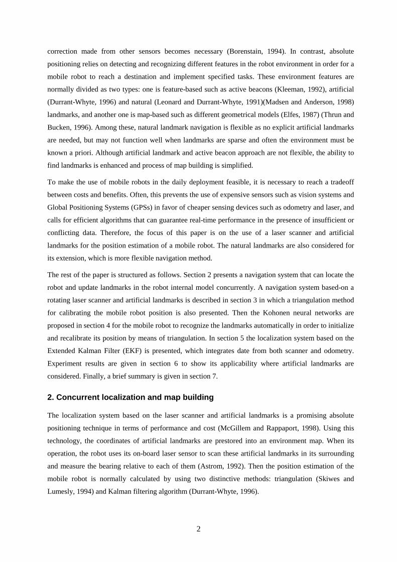
Figure 1 shows the block diagram of our navigation system that is able to implement concurrent
localization and map building automatically. It is a close-loop navigation process for position
initialization, position updating and map building.
Figure 1 Concurrent localization and map building
The system consists of three parts: an initialization part, an EKF part, and a map-building part. The
initialization part includes a triangulation algorithm, which is based on angle measurements from the
laser scanner. Kohonen Neural Networks are used here to identify the landmarks being detected and
achieve correct match between sensor data and the real world. The EKF part aims to fuse measuring
data from different sensors, and reduce individual sensor uncertainties. More details are presented in
section 4. In contrast, the task of the map building is to update and maintain the internal world model of
the mobile robot. A recursive least square algorithm is adopted to optimize the landmark position
LaserScanner
Sonarsensors
OpticalEncoders
Mobile Robot
AngleMeasurements
RangeReadings
OdometryCalculation
Triangulation Algorithm
Landmark Map
Matching? Updating
Prediction
Building Map
Estimated position
Initial position
Lost?Yes
No
Extended Kalman Filtering
Env
iron
men
t&
Lan
dmar
ks
Initialization
4
during operation of the mobile robot. The key idea is to optimize the internal landmark model during
the robot operation and add any natural landmark that is consistently detected by the laser scanner into
the localization process. The choice of the least square criteria is of course based on assumption that
measurement errors are Gaussian distribution.
3. Navigation system
3.1 Laser scanner and artificial landmarks
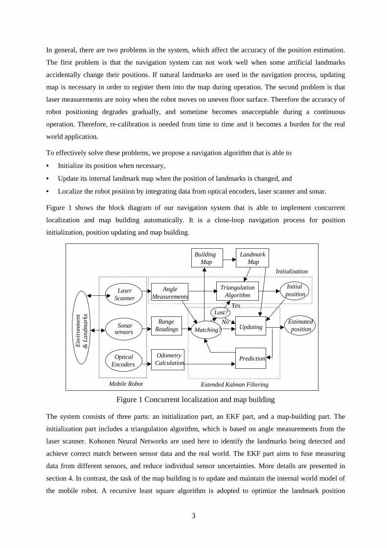
Research here is based on an industrial robotic system that uses artificial landmarks for localization. A
rotating laser scanner is used to measure the angle between the robot base line and the beam line from
either the leading or the falling edge of artificial landmarks in the horizontal plane. As shown in figure
2, the laser scanner is situated on the top of the physical center of the robot, scanned 360° in azimuth up
to 50m range at a constant speed of 2Hz. Note that an infrared laser beam (870nm) from a HeNe laser
diode emits energy of 0.5 mw, which is eye safe. As can be seen, there are 6 landmarks in this
environment, namely 621 ,...,, BBB .
Figure 2 Landmarks and an on-board laser scanner
The landmarks are currently in the form of single strip for easy detection at a long distance, instead of
traditional bar-coded. All landmarks have an identical size of 50cm in length and 10cm in width. The
positions of landmarks are surveyed in advance and pre-stored into the robot memory in a format of the
looking-up table, represented by the coordinates in the world frame:
where ),( yixi bb is the coordinates of the i'th landmarks and N is the total number of landmarks in use.
These landmarks can return strong reflective signals to the scanner, i.e. the area inside dotted lines in
figure 2. The reflected light from these landmarks is measured by a photodetector inside the scanner.
The scanner outputs the relative angles (with respect to the robot frame) measured by the scanner
encoder at the falling edge of each landmark. The measurement variance would increase when the
)1(),...],(),...,,[(],...,...,[ 111 yixiyxNi bbbbBBB ==ℜ
B1
B6
B5
B3
B2
B4
Mobile Robot
5
mobile robot moves around. This is because the vibration of the laser scanner would appear when the
floor surface is not smooth.
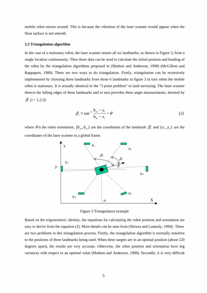
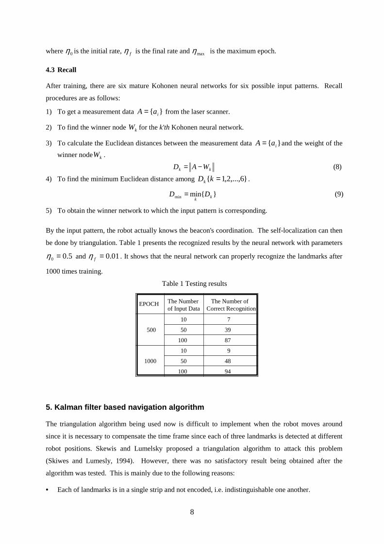
3.2 Triangulation algorithm
In the case of a stationary robot, the laser scanner senses all six landmarks, as shown in Figure 3, from a
single location continuously. Then these data can be used to calculate the initial position and heading of
the robot by the triangulation algorithms proposed in (Madsen and Anderson, 1998) (McGillem and
Rappaport, 1988). There are two ways to do triangulation. Firstly, triangulation can be recursively
implemented by choosing three landmarks from those 6 landmarks in figure 3 in turn when the mobile
robot is stationary. It is actually identical to the "3 point problem" in land surveying. The laser scanner
detects the falling edges of three landmarks and in turn provides three angle measurements, denoted by
iβ (i = 1,2,3):
)2(tan 1 θβ −−−
= −
lxi
lyii xb
yb
where θ is the robot orientation, ),( yixi bb are the coordinates of the landmark iβ and ),( ll yx are the
coordinates of the laser scanner in a global frame.
Figure 3 Triangulation example
Based on the trigonometric identity, the equations for calculating the robot position and orientation are
easy to derive from the equation (2). More details can be seen from (Skiwes and Lumesly, 1994). There
are two problems in this triangulation process. Firstly, the triangulation algorithm is normally sensitive
to the positions of three landmarks being used. When three targets are in an optimal position (about 120
degrees apart), the results are very accurate. Otherwise, the robot position and orientation have big
variances with respect to an optimal value (Madsen and Anderson, 1998). Secondly, it is very difficult
X
Y
xl
yl θ
β1
β2
b3
b4b5
b6
b2
b1
6
to identify which landmark has been detected if all landmarks are identical. Mismatch is more likely to
happen in practice when obstacles obscure one or more landmarks in the robot surroundings.
Alternatively, we can use all landmarks to make a least square solution with redundant observations so
that the individual solutions do not depend on the specific choice of the landmarks. This solution is non-
linear, and however, the equations can readily be linearized and used with the standard least square
algorithm. The advantage of this approach is that the redundant observations can be used to check and,
hopefully, eliminate blunders in the observation automatically (misidentification of the targets, etc.)
This approach can readily be automated and is, indeed, very popular in surveying. But it needs more
computation time comparing with the first approach.
4. Kohonen neural network for landmark detection
Since the laser scanner can only measure the angles to the different landmarks, and cannot distinguish
one landmark from another, a key problem is how to determine the correspondence between the
measured angle and the landmark (Astrom, 1992). Therefore, the initialization of the robot position is
normally done manually. Also, re-calibration is done manually when the mobile robot gets lost. This is
not convenient for real-world applications. It is necessary to find a feasible way to initialize the position
of a mobile robot automatically, which is addressed in this section.
4.1 Kohonen neural networks Kohonen neural networks have a structure arranged in a linear or planar manner, guided in particular by
finding in neurobiology. Their adjacent neurons react to similar stimuli that come from the natural
environment and are perceived by the sense organs. This algorithm is an unsupervised technique, and
also called self-organizing feature map (Fukushima et al., 1983). When the algorithm has converged,
the prototype vectors corresponding to nearby points on the feature map grid have nearby locations in
input space. It has been used in the self-localization process for a mobile robot (Janet et al., 1995).
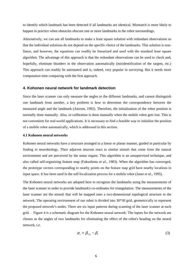
The Kohonen neural networks are adopted here to recognize the landmarks using the measurements of
the laser scanner in order to provide landmark's co-ordinates for triangulation. The measurements of the
laser scanner are the stimuli that will be mapped onto a two-dimensional topological structure in the
network. The operating environment of our robot is divided into 30*30 grid, geometrically to represent
the proposed network’s nodes. There are six input patterns during scanning of the laser scanner at each
grid. . Figure 4 is a schematic diagram for the Kohonen neural network. The inputs for the network are
chosen as the angles of two landmarks for eliminating the effect of the robot's heading on the neural
network, i.e.
)3(1 iii ββα −= +
7
So, there are five inputs in the network and six input patterns for six landmarks. The robot can get one
of the six input patterns during each scanning circle at each grid. We built up six networks to
correspond to the six input patterns. During training stage, six networks are trained according to the six
input patterns from laser scanner located in different grids respectively. When the neural networks
mature, the input patterns can be recognized by the corresponding network that has minimum summary
of the Euclidean distance between the network's weights and the input pattern.
Figure 4 Kohonen neural network
4.2 Training the network The Winner-Take-All learning algorithm is adopted here to train the parameters for the Kohonen neural
networks to locate the robot. Assume that the network weights are Wij, and the input data is A={ai} ,
where i=1,2,…, 5, j=1,2,…,30 for six landmarks situation in this research. The winner node WN is
determined by
The winner node and its neighbors are updated by
where ε is the epoch of the learning, εη is the learning rate parameter and εN is the neighborhood
size at the given epoch.
The learning rate and the neighborhood size are adapted with the epoch as follows
)4(min,
ijji
N WAWA −=−
)5(),()()1( εεη NnWAkWkW nnn ∈−+=+
)7(
4
12
1
4
12
1
1
3
5
max
maxmax
max
εε
εεε
εε
ε
<
<<
<
��
��
�
=N
)6(0max
0 ηεε
ηηηε −
−= f
54321 ααααα
8
where 0η is the initial rate, fη is the final rate and maxη is the maximum epoch.
4.3 Recall
After training, there are six mature Kohonen neural networks for six possible input patterns. Recall
procedures are as follows:
1) To get a measurement data }{ iaA = from the laser scanner.
2) To find the winner node kW for the k'th Kohonen neural network.
3) To calculate the Euclidean distances between the measurement data }{ iaA = and the weight of the
winner node kW .
4) To find the minimum Euclidean distance among }6,...,2,1{ =kDk .
5) To obtain the winner network to which the input pattern is corresponding.
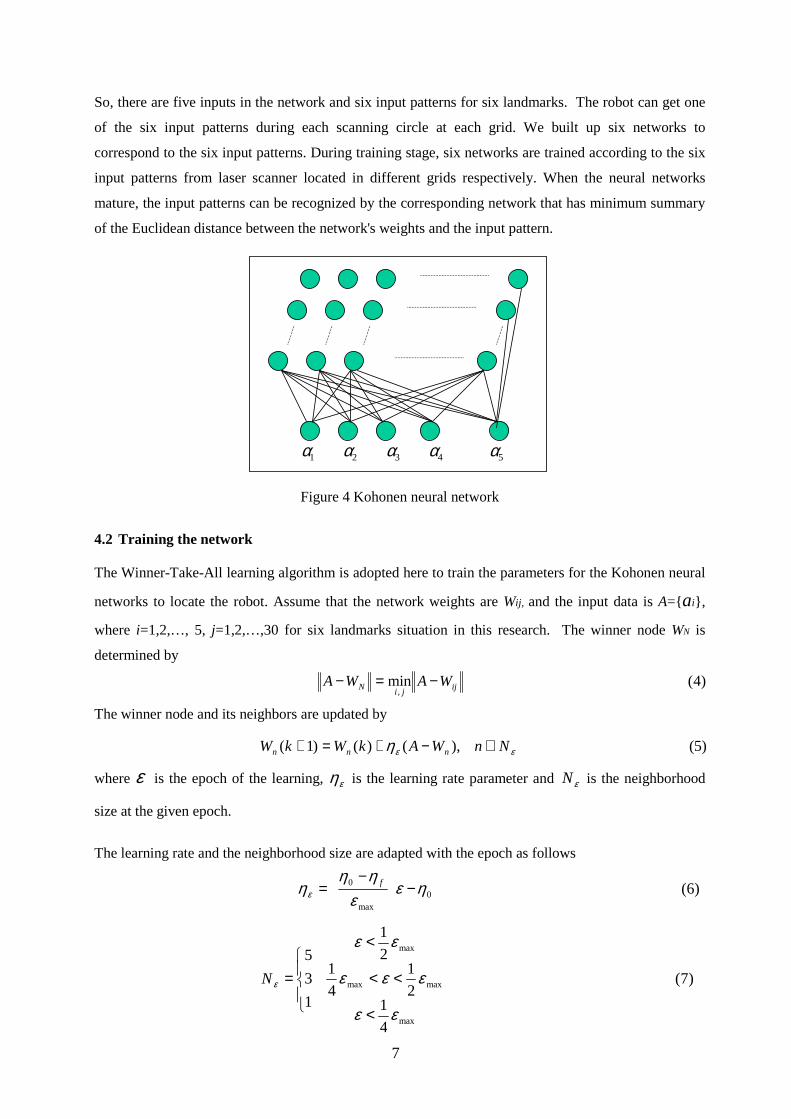
By the input pattern, the robot actually knows the beacon's coordination. The self-localization can then
be done by triangulation. Table 1 presents the recognized results by the neural network with parameters
5.00 =η and 01.0=fη . It shows that the neural network can properly recognize the landmarks after
1000 times training.
Table 1 Testing results
5. Kalman filter based navigation algorithm
The triangulation algorithm being used now is difficult to implement when the robot moves around
since it is necessary to compensate the time frame since each of three landmarks is detected at different
robot positions. Skewis and Lumelsky proposed a triangulation algorithm to attack this problem
(Skiwes and Lumesly, 1994). However, there was no satisfactory result being obtained after the
algorithm was tested. This is mainly due to the following reasons:
• Each of landmarks is in a single strip and not encoded, i.e. indistinguishable one another.
)8(kk WAD −=
)9(}{minmin kk
DD =
EPOCH The Number of Input Data
The Number ofCorrect Recognition
500
1000
10
50
100
10
50
100
7
39
87
9
48
94
9
• Noisy readings come from the laser scanner as some angle measurements are caused by random
objects.
• In general, the robot environment is non-convex. Therefore, not all landmarks can be seen by the
laser scanner. Moreover some landmarks may be obscured by dynamic objects such as humans and
other robots.
Therefore, the Extended Kalman Filter (EKF) has been used in the localization process (Leonard and
Durrant-Whyte, 1991), which is addressed here. The Kalman filter algorithm is a natural choice for
robot localisation since it provides a convenient way to fuse the data from multiple sensors, e.g. the
laser scanner and odometry in this work. However, it normally requires a linear dynamic model and a
linear output model. However, in this research, both models are nonlinear as follows:
where f(x(k), u(k)) is the nonlinear state transition function of the robot. w(k) ~ N(0, Q(k)) indicates a
Gaussian noise with zero mean and covariance Q(k). h(Bi, x(k)) is the nonlinear observation model and
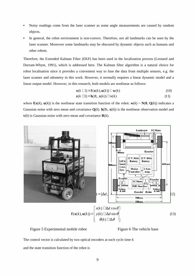
v(k) is Gaussian noise with zero mean and covariance R(k).
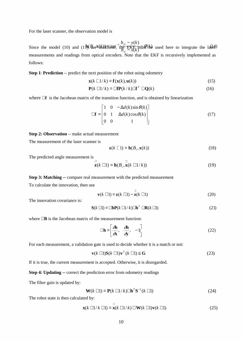
Figure 5 Experimental mobile robot Figure 6 The vehicle base
The control vector is calculated by two optical encoders at each cycle time k:
and the state transition function of the robot is
)12(],[)( Tdk θ∆∆=u
)13(
)(
sin)(
cos)(
))(),((
���
�
�
���
∆+∆+∆+
=θθ
θθ
k
dky
dkx
kk uxf
)11()())(,()1(
)10()())(),(()1(
kkBk
kkkk
i vxhz
wuxfx
+=++=+
10
For the laser scanner, the observation model is
Since the model (10) and (11) are nonlinear, the EKF must be used here to integrate the laser
measurements and readings from optical encoders. Note that the EKF is recursively implemented as
follows:
Step 1: Prediction -- predict the next position of the robot using odometry
where ∇f is the Jacobean matrix of the transition function, and is obtained by linearization
Step 2: Observation -- make actual measurement
The measurement of the laser scanner is
The predicted angle measurement is
Step 3: Matching -- compare real measurement with the predicted measurement
To calculate the innovation, then use
The innovation covariance is:
where ∇B is the Jacobean matrix of the measurement function:
For each measurement, a validation gate is used to decide whether it is a match or not:
If it is true, the current measurement is accepted. Otherwise, it is disregarded.
Step 4: Updating -- correct the prediction error from odometry readings
The filter gain is updated by:
The robot state is then calculated by:
)14()()(
)(tan))(,( 1 k
kxb
kybkB
xi
yii θ−
−−
= −xh
)17(
100
)(cos)(10
)(sin)(01
���
�
�
���
∆∆−
=∇ kkd
kkd
θθ
f
)18())(,()1( kBk i xhz =+
)19())/1(,()1( kkBk i +=+∧∧xhz
)20()1()1()1( +−+=+∧
kkk zzv
)16()()/()/1(
)15())(),(()/1(
kkkkk
kkkkT QffPP
uxfx
+∇∇=+
=+
)21()1()/1()1( ++∇+∇=+ kkkk T RhhPS
)22(1,, ��
��
−=∇
yh
xh
h∂∂
∂∂
)23()1()1()1( GvSv ≤+++ kkk T
)24()1()/1()1( 1 +∇+=+ − kkkk TShPW
)25()1()1()/1()1/1( ++++=++∧
kkkkkk vWxx
11
The covariance is updated by:
Step 5: Return to Step 1 to recursively implement four steps above.
The algorithm is essentially very simple although it hides some very useful features. It produces the
estimate of the current robot position at each cycle by integrating odometry data with only one angle
measurement from the laser scanner. Recursively, it combines every new measurement with
measurements made in the past to estimate the robot position, or "make a compromise". This can be
seen as a pseudo "triangulation" technique in a dynamic sense.
6. Experimental results
The proposed algorithm was implemented in our car-like mobile robot (Hu and Brady, 1997). As shown
in figure 5, the mobile robot has four wheels with pneumatic tyres, measuring 100cm (length) x 60cm
(width) x 120cm (height). It has a weight of 100kg and a maximum speed of 1m/s. Two front wheels
serve for steering and two rear wheels serve for traction. Incremental encoders (two 500
count/revolution) are fixed onto two rear wheels via 3:1 ratio pulley and belts. More detailed
configuration can be seen from figure 6.
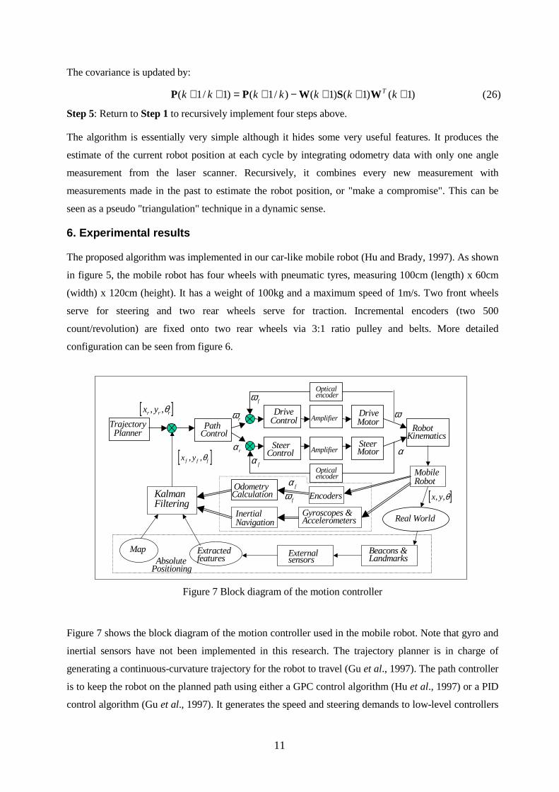
Figure 7 Block diagram of the motion controller
Figure 7 shows the block diagram of the motion controller used in the mobile robot. Note that gyro and
inertial sensors have not been implemented in this research. The trajectory planner is in charge of
generating a continuous-curvature trajectory for the robot to travel (Gu et al., 1997). The path controller
is to keep the robot on the planned path using either a GPC control algorithm (Hu et al., 1997) or a PID
control algorithm (Gu et al., 1997). It generates the speed and steering demands to low-level controllers
PathControl
Drive Control
SteerControl
Amplifier
Amplifier
DriveMotor
SteerMotor
Robot Kinematics
Opticalencoder
Opticalencoder
OdometryCalculation
α
ω f
α f
ωr
αr
ω f
α f
Real World
ω
MobileRobot
Encoders
Gyroscopes &Accelerometers
InertialNavigation
KalmanFiltering
[ ]x yr r r, ,θ
[ ]x yf f f, ,θ
[ ]x y, ,θ
Beacons &Landmarks
Map Extractedfeatures
Externalsensors Absolute
Positioning
Trajectory Planner
)26()1()1()1()/1()1/1( +++−+=++ kkkkkkk TWSWPP
12
based on errors between the desired trajectory and the actual trajectory estimated by the EKF. A PID
control algorithm has been used in the drive and steering controllers for maintaining stable speed and
steering angle.
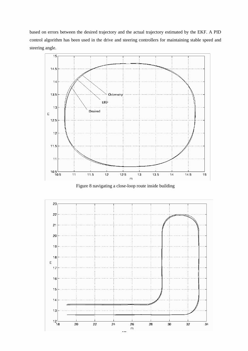
Figure 8 navigating a close-loop route inside building
13
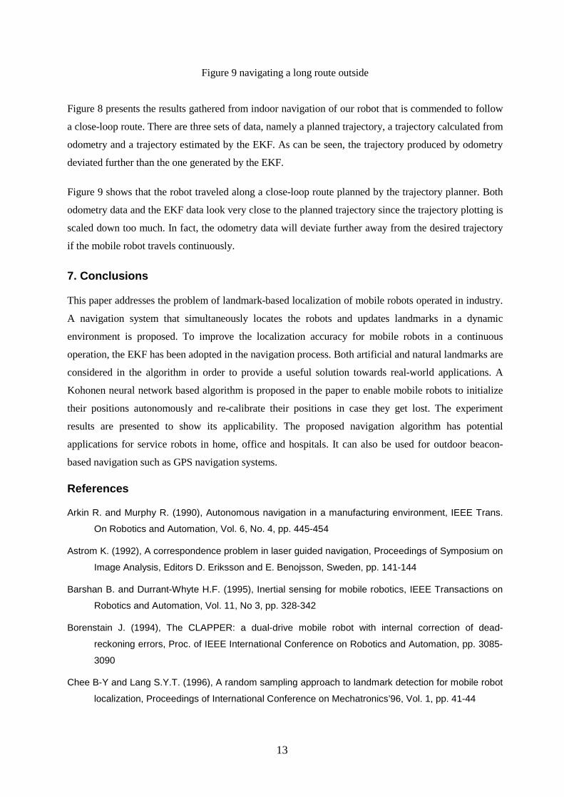
Figure 9 navigating a long route outside
Figure 8 presents the results gathered from indoor navigation of our robot that is commended to follow
a close-loop route. There are three sets of data, namely a planned trajectory, a trajectory calculated from
odometry and a trajectory estimated by the EKF. As can be seen, the trajectory produced by odometry
deviated further than the one generated by the EKF.
Figure 9 shows that the robot traveled along a close-loop route planned by the trajectory planner. Both
odometry data and the EKF data look very close to the planned trajectory since the trajectory plotting is
scaled down too much. In fact, the odometry data will deviate further away from the desired trajectory
if the mobile robot travels continuously.
7. Conclusions
This paper addresses the problem of landmark-based localization of mobile robots operated in industry.
A navigation system that simultaneously locates the robots and updates landmarks in a dynamic
environment is proposed. To improve the localization accuracy for mobile robots in a continuous
operation, the EKF has been adopted in the navigation process. Both artificial and natural landmarks are
considered in the algorithm in order to provide a useful solution towards real-world applications. A
Kohonen neural network based algorithm is proposed in the paper to enable mobile robots to initialize
their positions autonomously and re-calibrate their positions in case they get lost. The experiment
results are presented to show its applicability. The proposed navigation algorithm has potential
applications for service robots in home, office and hospitals. It can also be used for outdoor beacon-
based navigation such as GPS navigation systems.
References
Arkin R. and Murphy R. (1990), Autonomous navigation in a manufacturing environment, IEEE Trans.
On Robotics and Automation, Vol. 6, No. 4, pp. 445-454
Astrom K. (1992), A correspondence problem in laser guided navigation, Proceedings of Symposium on
Image Analysis, Editors D. Eriksson and E. Benojsson, Sweden, pp. 141-144
Barshan B. and Durrant-Whyte H.F. (1995), Inertial sensing for mobile robotics, IEEE Transactions on
Robotics and Automation, Vol. 11, No 3, pp. 328-342
Borenstain J. (1994), The CLAPPER: a dual-drive mobile robot with internal correction of dead-
reckoning errors, Proc. of IEEE International Conference on Robotics and Automation, pp. 3085-
3090
Chee B-Y and Lang S.Y.T. (1996), A random sampling approach to landmark detection for mobile robot
localization, Proceedings of International Conference on Mechatronics’96, Vol. 1, pp. 41-44
14
Durrant-Whyte H.F. (1996), An autonomous guided vehicle for cargo handling applications,
International Journal of Robotics Research, Vol. 15, No. 5, pp. 407-440
Elfes A. (1987), Sonar-based real-world mapping and navigation, IEEE Journal of Robotics and
Automation, RA-3 (3), pp. 249-265
Fukushima K., Miyake S., and Ito T. (1983), "Recognition: A neural network model for a mechanism of
visual pattern recognition", IEEE Transactions on Systems, Man and Cybernetics, Vol. SMC-13,
No.5, pp. 826-834
Gu D., Hu H., Brady M., Li F. (1997), Navigation System for Autonomous Mobile Robots at Oxford,
Proceedings of International Workshop on Recent Advances in Mobile Robots, Leicester, U.K.,
pp. 24-33
Hu H., Brady M., Probert P. (1993), Trajectory Planning and Optimal Tracking for an Industrial Mobile
Robot, Proceedings of SPIE's International Symposium on Mobile Robots VIII, Vol. 2058, Boston,
USA, pp. 152-163
Hu H. and Brady M. (1997), Dynamic Global Planning with Uncertainty for Autonomous Mobile Robots
in Manufacturing, IEEE Transactions on Robotics and Automation, Vol. 13, No. 5, pages 760-766
Hu H., Gu D., Brady M. (1998), A Modular Computing Architecture for Autonomous Robots, in the
International Journal of Microprocessors and Microsystems, Vol. 21, No. 6, pp. 349-362
Janet J.A., Gutierrez-Osuna R., Chase T.A., White M., Luo R.C. (1995), "Global self localization for
autonomous mobile robots using self-organizing Kohonen neural networks", Proceedings of
International Conference on Intelligent Robots and Systems, pp. 504-509
Kleeman L. (1992), Optimal estimation of position and heading for mobile robots using ultrasonic
beacons and dead reckoning, Proc. of IEEE Int. Conf. on Robotics and Automation, pp. 2582-
2587
Leonard J. and Durrant-Whyte H. (1991), Mobile robot localization by tracking geometric beacons, IEEE
Transactions on Robotics and Automation, Vol. 7, pp. 376-382
Madsen C.B. and Andersen C.S. (1998), Optimal landmark selection for triangulation of robot position,
International Journal of Robotics and Autonomous Systems, Vol. 23, No. 4, pp. 277-292
McGillem C.D. and Rappaport T.S. (1988), Infrared location system for navigation of autonomous
vehicles, Proceedings of International Conference on Robotics and Automation, pp. 1236-1238
Skewis T. and Lumesly V. (1994), Experiments with a mobile robot operating in a cluttered unknown
environment, Journal of Robotic Systems, 11(4), pp. 281-300
Thrun S. and Bucken A. (1996), Integrating grid-based and topological maps for mobile robot
navigation, Proceedings of the 13th National Conference on AI, Portland Oregon, pp. 128-133