land and soil monitoring: a guide for soe and regional - envirolink
TRANSCRIPT

Land and Soil Monitoring: A guide for SoE and regional council reporting 2009
Tips for using this document
Tips for using this document
Navigating the pdf The pdf has been set to open up with a Bookmark pane on the left hand side of the screen and a page view on the right.
Bookmarks are the easiest way to navigate this pdf on screen. Clicking on a bookmark will take you directly to the section indicated. For this reason, the guide’s Contents pages have not been bookmarked as the Bookmark pane is identical to the Contents pages and functions better than a Contents page with links would function1.
The Bookmarks are structured like a nested file directory i.e. sub-sections are below sections and sections are below chapters. To expand or collapse the nested structure, click on the plus or minus (+ or -) signs next to the Bookmark names.
Links have also been created where a website reference or a reference to another part of the guide appears. Your cursor will change to a pointing finger if you hover over these links and a click will take you to the website or page concerned. To return to your original position, use the Bookmarks pane.
You can also use Acrobat’s search function to find all references to a particular topic. On the menu bar select Edit/Search. A search pane will appear enabling you to enter the word or phrase you wish to find.
Printing This pdf file has been set up to print double-sided on A4 paper. For this reason blank pages have been inserted to enable each new chapter to start on a right hand page. You will need to specify double-sided printing (flip on long edge) in your printer settings.
The guide has also been structured to allow each chapter to be printed independently. Consequently, while there is a main table of contents at the beginning of the document, each chapter also has its own (more detailed) table of contents. For this reason appendices and references have also been kept with their associated chapters (rather than being collated at the end of the document).
To print:
The whole guide Print pages 3 to 178
Only Chapter 1: Overview Print pages 13 to 18
Only Chapter 2: Design of sampling programmes Print pages 19 to 38
1 Links in pdfs can only take you to a specified page whereas Bookmarks can take you to a specific section on a page.

Land and Soil Monitoring: A guide for SoE and regional council reporting 2009
Tips for using this document
Only Chapter 3: Soil quality monitoring Print pages 39 to 100
Only Chapter 4: Assessing soil stability Print pages 101 to 128
Only Chapter 5: Trace element monitoring Print pages 129 to 178
Copyright Please take note of the copyright conditions and referencing requirements for this guide (reproduced from the inside front cover of the document).
© 2009 Land Monitoring Forum
This document may be stored and distributed electronically and printed in-house or photocopied without prior permission of the publisher/copyright holder. However, its format cannot be altered and it cannot be sold in any form without the publisher/copyright holder’s permission.
If excerpts from this manual are used in other documents, they must be referenced according to the following format: Chapter author(s) last name, Chapter author(s) initials. Date. “Chapter title” in Land and Soil Monitoring: A guide for SoE and Regional Council Reporting; New Zealand.
Published by the Land Monitoring Forum, New Zealand.
Cover and divider photographs © 2004 Peter Singleton. Title page: Lismore. Chapter 1: Hamilton. Chapter 2: Te Kopuru. Chapter 3: Oamaru. Chapter 4: Kumara. Chapter 5: Te Kowhai.

Land and Soil Monitoring: A guide for SoE and regional council reporting
LANDMONITORINGFORUM

© 2009 Land Monitoring Forum
This document may be stored and distributed electronically and printed in-house or photocopied without prior permission of the publisher/copyright holder. However, its format cannot be altered and it cannot be sold in any form without the publisher/copyright holder’s permission.
If excerpts from this manual are used in other documents, they must be referenced according to the following format: Chapter author(s) last name, Chapter author(s) initials. Date. “Chapter title” in Land and Soil Monitoring: A guide for SoE and Regional Council Reporting; New Zealand.
Published by the Land Monitoring Forum, New Zealand.
Cover and divider photographs © 2004 Peter Singleton. Title page: Lismore. Chapter 1: Hamilton. Chapter 2: Te Kopuru. Chapter 3: Oamaru. Chapter 4: Kumara. Chapter 5: Te Kowhai.

Acknowledgements The Land Monitoring Forum thanks the following people and organisations for their contributions: The Ministry for the Environment for funding both the development of the
Soil Quality Monitoring chapter and the editing and formatting of the document (except Chapter 5).
Environment Waikato for funding the editing and formatting of Chapter 5. Wayne Smith, Environment Bay of Plenty, who chaired the Land Monitoring
Forum over the years during which time the 500 Soils project was implemented and reviewed and these guidelines were developed.
Wayne Bettjeman, Kirsty Johnston, Brent King and Justine Daw who have supported the ongoing development of this work and the objectives of the Land Monitoring Forum over the years.
Chris Frampton, statistician, who provided valued advice on sampling design for monitoring soil quality and soil stability.
Jeremy Cuff and John Phillips for significant contributions to the content and editing of Chapter 3.
A number of people contributed to development of the point sample analysis procedure described in Chapter 4. Malcolm Todd, Tony Thompson, Peter Fantham, Reece Hill, Dave Cameron, and Wayne Smith encouraged its development and trial. Andrew Haig, Mark Williams, Tim Watson, Gareth Evans, Michelle Hosking, Myles Hicks and Dan Borman facilitated the method’s transition to a GIS-based procedure. Terry Crippen, Andrew Burton, Daimen Jones, Tony Thompson and Colin Gray have implemented various operational improvements while undertaking point samples. Amy Taylor has improved table layouts and report formats.
Northland Regional Council, Auckland Regional Council, Environment Waikato, Environment Bay of Plenty, Hawke’s Bay Regional Council, Taranaki Regional Council, Gisborne District Council, Horizons, Marlborough District Council, Tasman District Council, Environment Canterbury, and Southland Regional Council, for supporting their NLMF delegates and enabling them to contribute to these guidelines.
Groundwork Associates for their editing and desktop publishing assistance.


Land and Soil Monitoring: A guide for SoE and regional council reporting 2009
Table of Contents v
Contents Chapter 1: Overview.....................................................................................1 1 Introduction........................................................................................3
1.1 Environmental performance indicators: The Pressure-State-Response model .......... 3 1.2 Purpose and status of this guide....................................................................................... 4 1.3 Scope of this guide .............................................................................................................. 5
Chapter 2: Design of sampling programmes .............................................7 1 Introduction......................................................................................11 2 Setting objectives............................................................................11
2.1 Key elements...................................................................................................................... 11 2.2 Attributes............................................................................................................................ 12 2.3 Area ..................................................................................................................................... 13
3 Sampling ..........................................................................................13
3.1 Random representative sampling................................................................................... 13 4 Sample units.....................................................................................14
4.1 Area based units................................................................................................................ 14 4.2 Cluster point units ............................................................................................................ 15 4.3 Point units .......................................................................................................................... 15
5 Stratification .....................................................................................16 6 Trend monitoring..............................................................................17
6.1 Choosing sample units for trend monitoring................................................................ 17 6.2 Determining sampling frequency for trend monitoring ............................................. 17
7 Accuracy and precision.................................................................18
7.1 Accuracy ............................................................................................................................. 18 7.2 Precision ............................................................................................................................. 18 7.3 Sampling error................................................................................................................... 19
8 Pilot studies ......................................................................................20 9 Designing a monitoring programme - key considerations ........20 10 Case studies.....................................................................................22
10.1 Case Study 1: Ambient concentrations of selected organochlorides in soils............ 22 10.2 Case Study 2: Rural land use on Auckland soils .......................................................... 23 10.3 Case Study 3: 500 Soils ..................................................................................................... 24

Land and Soil Monitoring: A guide for SoE and regional council reporting 2009
Table of Contents vi
References...................................................................................................25 Additional reading......................................................................................25 Chapter 3: Soil quality monitoring .............................................................27 1 Introduction......................................................................................31 2 Why monitor soil quality?................................................................31 3 Why these soil quality indicators?..................................................32 4 Sample programme design ...........................................................36
4.1 Stratification....................................................................................................................... 36 4.2 Sample numbers (sample size, n).................................................................................... 39 4.3 Sampling frequency .......................................................................................................... 39 4.4 Time of collection .............................................................................................................. 40
5 Sampling methodology ..................................................................41
5.1 Site selection....................................................................................................................... 41 5.2 In-field sampling technique............................................................................................. 42
6 Laboratory methods........................................................................46
6.1 Laboratory selection.......................................................................................................... 47 6.2 Archive ............................................................................................................................... 47
7 Data interpretation ..........................................................................47
7.1 Total Carbon target ranges (%w/w) .............................................................................. 48 7.2 Total Nitrogen target ranges (%w/w) ........................................................................... 48 7.3 Mineralisable N target ranges (ug/g) ............................................................................ 49 7.4 pH target ranges................................................................................................................ 49 7.5 Olsen P target ranges........................................................................................................ 50 7.6 Bulk density target ranges (t/m3 or Mg/m3) ................................................................ 50 7.7 Macroporosity target ranges (-10 kPa) (%) .................................................................... 51
8 Data management and storage....................................................51 Appendix I ...................................................................................................52
Determining the number of nationally representative samples ........................................... 52 Appendix II ..................................................................................................54
Template for site management history..................................................................................... 54 Soil Quality Monitoring.............................................................................................................. 54
Appendix III .................................................................................................58
Required Laboratory Methods for Soil Quality Monitoring ................................................. 58 Soil preparation ........................................................................................................................... 58 Drying and grinding ................................................................................................................... 58 Moisture content method ........................................................................................................... 59

Land and Soil Monitoring: A guide for SoE and regional council reporting 2009
Table of Contents vii
Total C method ............................................................................................................................ 60 Total N method............................................................................................................................ 61 Mineralizable N method............................................................................................................. 62 Soil pH in water method ............................................................................................................ 64 Olsen P method ........................................................................................................................... 66 Bulk density method................................................................................................................... 66 Macroporosity method ............................................................................................................... 70
Appendix IV.................................................................................................81
The New Zealand Land Cover Database ................................................................................. 81 What is it and what can it be used for? .................................................................................... 81 Why was it created? .................................................................................................................... 81 Who will find it useful and why?.............................................................................................. 82 The land cover classes................................................................................................................. 83
References...................................................................................................86 Chapter 4: Assessing soil stability 89 1 Introduction 93
1.1 Definitions of indicators................................................................................................... 93 1.2 Point sample analysis ....................................................................................................... 94
2 Survey design 95
2.1 Measurement from aerial photographs ......................................................................... 95 2.2 A point sample on a topographic map grid .................................................................. 96
3 Recording data 98
3.1 Point identification number............................................................................................. 99 3.2 Grid reference .................................................................................................................... 99 3.3 Land use ............................................................................................................................. 99 3.4 Secondary vegetation...................................................................................................... 102 3.5 Land stability ................................................................................................................... 102 3.6 Nature of disturbance..................................................................................................... 103 3.7 Landform.......................................................................................................................... 104 3.8 Bare soil ............................................................................................................................ 105
4 Storing data 106
4.1 Recording data from conventional aerial photographs............................................. 106 4.2 Recording data from orthophotos ................................................................................ 106 4.3 Editing data...................................................................................................................... 106 4.4 Storing repeat data.......................................................................................................... 106
5 Data analysis 107
5.1 Data processing methods............................................................................................... 107 5.2 Types of analysis ............................................................................................................. 107 5.3 Summary tables ............................................................................................................... 108

Land and Soil Monitoring: A guide for SoE and regional council reporting 2009
Table of Contents viii
6 Statistical interpretation 108 6.1 Photo interpretation error .............................................................................................. 108 6.2 Sampling error................................................................................................................. 108 6.3 Precision of measurements ............................................................................................ 109 6.4 Sample representativeness............................................................................................. 110 6.5 Tests for significance of comparisons........................................................................... 111 6.6 Extracting sub-sets from regional data ........................................................................ 113
7 Documents, their use and environmental interpretation 113
7.1 Standard reports.............................................................................................................. 114 7.2 Report contents and focus.............................................................................................. 114
8 References 115 Chapter 5: Trace element monitoring.....................................................117 1 Introduction....................................................................................121 2 Basic concepts and definitions....................................................121
2.1 Trace elements ................................................................................................................. 121 2.2 Heavy metals ................................................................................................................... 121 2.3 Partitioning between soils and soil pore water........................................................... 122 2.4 Interpretation of reported results ................................................................................. 122 2.5 Relationship to contaminated land investigation....................................................... 124
3 General characteristics ................................................................125
3.1 Background and typical concentrations ...................................................................... 125 3.2 Essential and non-essential trace elements.................................................................. 128 3.3 Behaviour of trace elements in soils ............................................................................. 131 3.4 Sources of trace elements in productive soils ............................................................. 138
4 Sampling for trace elements ........................................................148
4.1 General approach and specific recommendations ..................................................... 148 5 Analysis ..........................................................................................150
5.1 What trace elements could be measured? ................................................................... 150 5.2 Types of extractions for measuring trace elements in soils....................................... 151 5.3 Common methods of analysis for trace elements....................................................... 153 5.4 Data interpretation.......................................................................................................... 154
6 References .....................................................................................165

Land and Soil Monitoring: A guide for SoE and regional council reporting 2009
List of figures and tables ix
List of figures and tables
Figures Title Page
Figure 1.1: The Pressure-State-Response model 3
Figure 2.1: Comparison of sample units. 5
Figure 2.2: Stratification according to area attributes. 6
Figure 2.3: Accuracy and precision. 8
Figure 4.1: NZMS 260 topographic map sheet grid with hectare square sample points centred on each 2km intersection overlaying an orthophoto.
98
Figure 4.2: Cluster sample of 100 dots around a sample point. 105
Figure 5.1: Relationship between health status and concentration for an essential element.
128
Figure 5.2: Relationship between health status and concentration for an essential element.
130
Figure 5.3: Functional groups that fix trace elements present in soil organic matter. 133
Figure 5.4: Inorganic hydroxyl groups on the goethite (α-FeO(OH)) surface. 133
Figure 5.5. A silicon oxide sheet. 134
Figure 5.6: Interrelationships between trace elements in organisms. 137
Figure 5.7: Processes involved in cycling of trace elements between the atmosphere, lithosphere and hydrosphere.
140
Figure 5.8: Flowchart showing steps to synthesis of nitrogen fertilisers. 145
Tables Title Page
Table 3.1: National soil quality monitoring indicators. 34-35
Table 3.2: Levels of land use classification for national and regional stratification. 37
Table 3.3: Soil stratification hierarchy. 38
Table 3.4: Primary Land Use Types for sampling. 38
Table 3.5: Recommended re-sampling frequencies for different land uses. 40
Table 3.6: Recommended procedures for analyses. 46
Table 3.7: Overall coefficients of variance of physical, chemical and biological properties used to measure soil quality. The variance is the sum of any systematic, spatial and land use effects.
52
Table 3.8: Preparing reagents for Mineralizable N method. 62
Table 3.9: Preparing buffers for Soil pH in water method. 64

Land and Soil Monitoring: A guide for SoE and regional council reporting 2009
List of figures and tables x
Table 3.10: Preparing reagents for Olsen P method. 66
Table 3.11: Preparing standards for Olsen P method. 67
Chapter 3 Appendix IV: Target Classes for Land Cover Database Version 84
Table 4.1: Error margins (at 95% confidence) associated with point count estimates for various sample sizes.
97
Table 4.2: Land use category codes. 100-101
Table 4.3: Secondary land use codes. 101
Table 4.4: Land stability codes. 102
Table 4.5: Soil disturbance codes. 103
Table 4.6: Landform codes. 104
Table 4.7: Landform codes for points lacking soil. 105
Table 5.1: Concentration ranges (mg/kg) of 13 trace elements in soils in different regions of New Zealand.
127
Table 5.2: Average background concentrations of 33 elements in Waikato soils (0-10 cm), ranked in decreasing concentration order.
129
Table 5.3: Essential major and trace elements for animal and plant health. 126
Table 5.4: Examples of fixation and release for applied soil cadmium. 136
Table 5.5: Concentration ranges (mg/kg) of selected trace elements in soil conditioners and fertilizers.
144
Table 5.6: Concentrations (mg/kg dry weight) of eight elements in garden composts tested by Environment Waikato.
145
Table 5.7: Concentrations (mg/kg dry weight) of eight elements in fertilisers tested by Environment Waikato.
146
Table 5.8: Copper and zinc loadings on soils under some common horticultural crops.
147-148
Table 5.9: Common instrumental methods used for analysis of trace elements. 153-154
Table 5.10: Common trace element deficiencies in plants. 156
Table 5.11: Background topsoil concentrations of trace elements published by regional councils.
158
Table 5.12: Guideline values for selected trace elements in agricultural soils. 159-164

Chapter 1
Overview

Land and Soil Monitoring: A guide for SoE and regional council reporting 2009
Overview 2

Land and Soil Monitoring: A guide for SoE and regional council reporting 2009
Overview 3
1 Introduction Section 35(2) (a) of the Resource Management Act 1991, places a legislative and administrative responsibility on regional councils to monitor and report on the state of the environment in their regions.
State of the Environment (SoE) monitoring measures and monitors human activities and their effects on the environment using environmental performance indicators. Over time environmental reporting will: raise the level of knowledge about the state of New Zealand’s environment; strengthen our ability to report on environmental health and trends; provide the tools for effective evaluation of policy; and establish the information base for more informed policy and management decisions.
To be powerful and informative, monitoring and reporting ideally needs to be nationally consistent. This requires agreed guidelines, including protocols and methods. To this end, the Land Monitoring Forum (LMF) has compiled this guide to help regional council staff undertaking land monitoring. LMF members are drawn from regional council staff throughout New Zealand and all have roles relating to land monitoring.
1.1 Environmental performance indicators: The Pressure-State-Response model The Pressure-State-Response (PSR) model (see Figure 1), provides a suitable framework for SoE monitoring and reporting. It has been applied in many other countries and is recognised as a useful framework for indicator development and reporting worldwide.
Figure 1: The Pressure-State-Response model
Pressures on the environment
National
Regional
Local
Global Central government
policies and actions Local government
policies and actions Community/sector
attitudes and actions Individual/household
attitudes and actions
Information
State of the environment and natural resources
Societal responses
Perceptions of the state of the environment
Direct pressures - Biological stresses
Indirect pressures - Human activities - Natural events

Land and Soil Monitoring: A guide for SoE and regional council reporting 2009
Overview 4
The Organisation for Economic Co-operation and Development first developed the PSR framework for environmental indicators. It is based on a concept of causality. Human activities exert pressures on the environment, changing both the quality and quantity of natural resources. These changes alter the state, or condition, of the environment. Human responses to these changes include any organised behaviour that aims to reduce, prevent or mitigate undesirable change or environmental results.
The PSR model asks three fundamental questions:
What are the pressures on the environment? This identifies environmental issues and their causes.
What is the state of the environment? This tells us what to monitor where, relative to the issues.
What is being done about these issues? This identifies policy goals and management actions for the issues.
Most regional councils have traditionally focused on the PSR model’s State indicators although some less well-resourced councils are only now starting to consider these in their monitoring programmes. State indicators require a particularly high level of scientific and statistical robustness, which this guide intends to address.
However, because of the rapidly changing pressures on New Zealand’s land environment (such as land use intensification), regional councils increasingly need to develop early warning indicators to help manage their land resource more proactively. While State indicators are extremely important in terms of councils’ environmental reporting commitments, Pressure indicators are arguably even more important in terms of councils’ commitments to effectively and sustainably manage the land resource into the future.
Pressure indicators – perhaps with the exception of Land Cover – are generally at an earlier stage of development than State indicators. Nevertheless, this guide outlines these indicators and their current status, as a benchmark and to earmark them for future development through the LMF.
For completeness the guide also includes chapters on topics for which protocol development has been more limited. This has the benefit of: highlighting where LMF should focus future effort in protocol development; and providing complete coverage of land aspects that require monitoring.
Therefore this guide is a living document and future updates can be expected as new methodologies develop and existing ones are refined.
1.2 Purpose and status of this guide The approaches in this guide are technically robust, based on the best available knowledge and information at this time. They have been through a rigorous process of expert design and extensive peer review, intended to remove the burden of technical justification that councils sometimes face.
The LMF’s intention, through this guide, is to widely promote the adoption of scientifically robust and consistent methodologies among regional councils. This has a range of benefits, the most obvious being to enable aggregation of land monitoring information to a national level. However – irrespective of national or international reporting requirements and commitments – there are significant benefits to regional councils in terms of aggregation (at least to multi-regional level) where similar land environments straddle a number of adjacent regions. This enables efficiencies such as shared use of reference sites for soil quality between adjacent regional councils and even aggregation of soil quality data on similar impacted sites

Land and Soil Monitoring: A guide for SoE and regional council reporting 2009
Overview 5
for comparison. This can give regional councils access to larger shared datasets which can increase the robustness and the ability to detect any trends in the data.
1.3 Scope of this guide This guide includes agreed approaches to the key aspects of land resource management in New Zealand.
Chapter 2: Design of sampling programmes. Covers the statistical and scientific requirements of effective monitoring programmes.
Chapter 3: Soil quality monitoring. Addresses national indicators, sampling design and methodology, laboratory methods, data interpretation and storage for soil quality monitoring.
Chapter 4: Assessing soil stability. Outlines use of point sampling analysis to estimate the state of soil disturbance and its change over time.
Chapter 5: Trace element monitoring. Examines the character, behaviour and interaction of inorganic trace elements; issues arising from their accumulation and recommendations for sampling programme design, data analysis and interpretation.
As stated previously, this guide simply reflects agreed best practice. Regional councils may choose to adapt their approach according to regionally relevant factors such as resourcing capability, priorities and needs in relation to other competing issues. However, in doing so they must weigh up the advantages and disadvantages of any variation.
The LMF encourages the adoption of the approaches in this guide and welcomes feedback on their use and future development.
Feedback on this guide should be addressed to:
The Convenor Land Monitoring Forum [email protected]

Land and Soil Monitoring: A guide for SoE and regional council reporting 2009
Overview 6

Chapter 2
Design of sampling programmes
Author: C. Frampton.

Land and Soil Monitoring: A guide for SoE and regional council reporting 2009
Design of Sampling Programmes 8.

Land and Soil Monitoring: A guide for SoE and regional council reporting 2009
Design of Sampling Programmes 9.
Contents 1 Introduction ..................................................................................... 11
2 Setting objectives ........................................................................... 11
2.1 Key elements.......................................................................................................................11
2.2 Attributes ............................................................................................................................12
2.2.1 Direct attributes..................................................................................................................12 2.2.2 Indirect attributes...............................................................................................................12
2.3 Area......................................................................................................................................13
3 Sampling.......................................................................................... 13
3.1 Random representative sampling....................................................................................13
3.1.1 Simple random sampling..................................................................................................13 3.1.2 Systematic random sampling...........................................................................................13
4 Sample units .................................................................................... 14
4.1 Area based units.................................................................................................................14
4.1.1 ‘Weighting’ of area units...................................................................................................14 4.2 Cluster point units .............................................................................................................15
4.3 Point units ...........................................................................................................................15
5 Stratification..................................................................................... 16
6 Trend monitoring............................................................................. 17
6.1 Choosing sample units for trend monitoring ................................................................17
6.2 Determining sampling frequency for trend monitoring ..............................................17
7 Accuracy and precision ................................................................ 18
7.1 Accuracy..............................................................................................................................18
7.2 Precision ..............................................................................................................................18
7.3 Sampling error....................................................................................................................19
7.3.1 Formula for calculating sampling units..........................................................................19 8 Pilot studies...................................................................................... 20
9 Designing a monitoring programme - key considerations ....... 20
10 Case studies.................................................................................... 22
10.1 Case Study 1: Ambient concentrations of selected organochlorides in soils
(Buckland, S.J., Ellis, H.K and Salter, R.T.; (1998)) ........................................................22
10.2 Case Study 2: Rural land use on Auckland soils (Hicks, D.L. (2000)) ........................23
10.3 Case Study 3: 500 Soils (MfE Project Number 5089*)....................................................24
References .................................................................................................. 25
Additional reading ..................................................................................... 25

Land and Soil Monitoring: A guide for SoE and regional council reporting 2009
Design of Sampling Programmes 10.

Land and Soil Monitoring: A guide for SoE and regional council reporting 2009
Design of Sampling Programmes 11.
1 Introduction This chapter defines, explains and justifies the statistical and scientific requirements of effective monitoring programmes. It deals exclusively with establishing a monitoring protocol to efficiently describe soil and land attributes. It does not provide the information necessary to develop a specific experimental design to address putative cause-effect relationships.
Monitoring provides descriptive information on the current state of attributes or provides longitudinal data on the trends or relative trends of these attributes. Without experimental manipulation of sites/plots and adequate replication it cannot resolve cause-effect dilemmas. In many circumstances it seems expedient to address these dilemmas with single time-point or temporal monitoring. However, the confounding among multi-causal agents means that such studies are inherently flawed.
For example: You wish to explore the association between grazing intensity and soil quality properties by locating sites with varying grazing histories and then measuring their soil quality. The grazing histories are very likely to be linked (confounded) with other soil measures (moisture, nutrients, drainage, fertility etc.) which make these areas appropriate for higher grazing intensities. Therefore, the simple effects of grazing on soil quality cannot be determined.
When it is not possible to use an ideal monitoring programme design (for example, due to resource constraints), the compromises need to be identified. You must consider whether a sub-optimal design will actually provide the appropriate information to usefully address your objective(s). To achieve this you need to clearly and explicitly define your objectives.
2 Setting objectives Before you develop your monitoring programme, you need an explicit statement of the objectives(s). Keep referring to your objective(s) as you develop your protocol to ensure that the protocol will address them. If you have a number of objectives then state and prioritise all of them.
As you develop your monitoring protocol, you will need to make key decisions at each step. Making the ‘correct’ decision usually depends on maintaining the link between the monitoring protocol and your objectives.
2.1 Key elements Two key elements required within an objective are: explicit statements of the attributes or processes to be measured, the area within which they are to be measured.

Land and Soil Monitoring: A guide for SoE and regional council reporting 2009
Design of Sampling Programmes 12.
2.2 Attributes General statements about soil or water quality lack sufficient detail for an objective. So, for example, BOD, nitrate levels or other measures should be explicitly stated within the objective as indices/measures of quality. Additionally, the units associated with these measures should be clearly defined. This is particularly important when attributes or processes are assessed from randomly sampled management units (e.g. farms or fields) rather than areas. (e.g. % erosion/ha, or % erosion/farm).
Attributes tend to fall into one of two possible types: direct and indirect attributes.
2.2.1 Direct attributes Direct attributes are those where the measurements made have an intrinsic interpretation relevant to the primary monitoring objective. For example, if pH, top-soil depth or BOD are being measured and no further interpretation apart from the levels per-se is intended, then these are direct attributes.
Direct attributes are prone to being ‘over-interpreted’, e.g. a low pH or shallow top-soil being interpreted as indicative of depleted or degraded soils.
2.2.2 Indirect attributes Frequently the specific attributes of interest are not readily amenable to monitoring (e.g. erosion). In these situations, it is customary to assess ‘practices’ (e.g. cultivation) or surrogates (e.g. top-soil depth) which are believed to impact on or be related to the attribute of interest. It is then inferred that changes in practices or surrogates will directly relate to changes in the attributes of interest.
If carried out appropriately, monitoring practices will enable you to make valid conclusions on the status of attributes. However, you need to fully quantify the inferred association of practices with attributes (e.g. stocking levels with nitrates or soil compaction) before you can draw any conclusions about the attributes. The relationship between attributes and practices is likely to be non-linear, so you will not be able to directly equate proportional changes in practices to changes in attributes.
Designs that adequately quantify the cause-effect relationship between processes and attributes are complicated. The relationship needs to be established over a full range of practice intensities over appropriate time intervals. To construct these combinations and monitor impacts on attributes over time, it is important that the attributes’ baseline levels are comparable and that the combinations are replicated over an adequate range of environmental conditions.
This elaborate prospective monitoring programme design is unlikely to appeal in many situations, as it takes time to deliver results and is likely to be very expensive. To overcome this problem and establish the association between the practice and the attribute, it is common to use cross-sectional monitoring of attributes and relate this to historical information on exposure to the process. While this approach is attractive, it has strong potential for confounding between the historical processes and other management or environmental issues. For example, areas which have been frequently cultivated may also have more fertile soils and may have been exposed to other forms of intensive management.

Land and Soil Monitoring: A guide for SoE and regional council reporting 2009
Design of Sampling Programmes 13.
These concerns also apply when interpreting surrogate levels. Is there a direct relationship between the surrogate and the attribute? When different areas are being compared were they comparable prior to any management procedure or interference?
2.3 Area Your objective should also state and justify, the exact area to be sampled. Merely defining a general geographic locality (e.g. Nelson) does not allow for the inevitable complications associated with any sampling area (e.g. accessible, non-urban, >500 ASL). These specifics will also usually involve exact statements on the small-scale requirements for sampling units (e.g. soil cores to be taken where soil depth is > 10 cm) so that the exact horizon to be sampled, and any other requirements, are explicitly defined. Decisions on these specific requirements must be appropriately melded with the study objectives. If logistics/resource limitations dictate that only certain samples can be taken, then this point should be reflected in the study objectives.
3 Sampling
3.1 Random representative sampling For soil and land monitoring it is not usually feasible to measure attributes throughout the entire monitoring area (i.e. take a census). Therefore, samples must be taken from the monitoring area and the results from these samples presumed to represent the whole area. A common exception to this is where you can monitor attributes or practices from aerial photographs of the entire area. Whatever sampling method you use, you must maintain clear records of the GPS/Grid references chosen. The scale of the GPS/Grid references should reflect the size of the sampling units. For more about aerial assessment of attributes see Chapter 4: Survey design - photography. Two methods for selecting representative samples are described below.
3.1.1 Simple random sampling This method is the most likely to produce a genuinely representative sample. With simple random sampling, all units within the monitoring area have the same probability of being selected in the sample. One method of selecting random sampling units is to create grid squares over a map of the monitoring area and randomly select x and y coordinates that fall within the area.
A disadvantage of the simple random sample is that it is likely to be inefficient to locate and sample the selected units.
3.1.2 Systematic random sampling Where simple random sampling is impossible or inefficient, a standard compromise is to locate random transects (random starting and random bearings) throughout the area and position monitoring points systematically (at regular intervals) along these transects.

Land and Soil Monitoring: A guide for SoE and regional council reporting 2009
Design of Sampling Programmes 14.
An extension to this method, particularly where data are sampled from aerial photographs, is to overlay a grid system on a map of the area and sample at each intersection point.
These systematically random approaches have logistical advantages over simple random sampling. However, they rely on the following assumptions: sample units are independent of each other; and positioning monitor points at regular intervals does not lead to non-
representative sampling by coinciding with systematic variation in the measured attributes (e.g. ridges tend to systematically coincide with the spacing defined between units and are therefore over-sampled).
4 Sample units There may be many options available when selecting sample units to monitor individual attributes. Some attributes/processes lend themselves to area based units (e.g. erosion and land-use). Others suit point or cluster point units (e.g. levels within soil or water strata).
There are three sampling possibilities described below: area based units, cluster point units and point units (see Figure 2.1).
4.1 Area based units When areas are considered appropriate, the main consideration is the size of the sample unit. The final size is usually a compromise between the need for areas large enough to allow you to accurately assess proportions in different categories, (e.g. land-use) and yet small enough to enable you to delimit the area and assess it in a reasonable time.
Additional considerations include the efficiencies associated with different combinations of sample unit size and number. If there is a significant cost associated with locating each sample unit, then select fewer, larger units. If the primary cost is in the assessment of the area and location costs are minimal, then select more, smaller units.
4.1.1 ‘Weighting’ of area units When sampling units comprise areas rather than points, it is sometimes convenient to choose sample units of differing sizes, particularly when ‘use’ is being monitored with management units, e.g. fields.
The key issue associated with this is when results are expressed in terms of area rather than management units.
For example, if you are monitoring poor cultivation practices and assessing them at the field (management unit) level but want to express results per unit area. Rather than stating what percentage of the fields is poorly cultivated, you need to state what percentage of the area is poorly cultivated.
In these circumstances it is not adequate to express the result for each sample unit in terms of area and then average these and derive measures of variation from them. When you calculate the mean and variation, each sample unit must be weighted in

Land and Soil Monitoring: A guide for SoE and regional council reporting 2009
Design of Sampling Programmes 15.
direct proportion to each area sampled. For example, two fields of twenty and two hectares do not contribute equally in the calculation of the percentage of the area that is poorly cultivated.
4.2 Cluster point units Cluster point units are where more than one point is sampled within each sampling area. For example, fields are selected and a number of soil cores are taken from each field to estimate a single attribute value for the field. The rationale for sampling more than one point is to obtain a precise estimate of the attribute for each sample.
The number of points chosen for each unit is largely determined by the relative costs of locating the sampling units and taking each additional point within the unit. An additional and equally important consideration is the variability of the attributes within the sample unit. The greater the variability the more points required.
4.3 Point units Point units take single assessments at each randomly located position. When taking these samples, you must ensure that the exact location (e.g. position for a soil core) is randomly selected. This avoids the conscious or subconscious selection of units which are favourable for sampling within the larger randomly selected area. This consideration also applies to selecting individual points within clusters.
Figure 2.1: Comparison of sample units.
Note: In this example the cluster points units have six replicates, whereas the single point units have fifteen. There will be less variation among the six replicates (each has a mean of six pseudo-reps) from the cluster sampling than among the fifteen single point replicates.
X X
X
X X
X X
X X
X X
X
X X X
Point units Area based units Cluster point units
xxxxxx
xxxxxx
xxxxxx
xxxxxx
xxxxxx
xxxxxx

Land and Soil Monitoring: A guide for SoE and regional council reporting 2009
Design of Sampling Programmes 16.
5 Stratification Stratification is the process of subdividing a monitoring area to maximise differences in the attributes of interest between strata and minimise variation within each stratum. A stratum is an area in which the attribute being measured is relatively homogenous and usually there are profound differences in the attribute between strata. Strata are then sampled with sufficient replication of sampling units so that generalisations may be made about each.
Stratification serves two related purposes: it enables generalisations to be made about each stratum. This assumes that
the inherent differences between strata would make statements regarding all strata combined largely irrelevant.
it separates the inherent differences between strata from the variation among the sample units. This means attribute estimates will be more precise and the confidence intervals associated with the estimates will be smaller.
Stratification can effectively reduce the sample sizes required for specific levels of statistical confidence.
Usually stratification can be planned prior to sampling so that adequate replication can be used for each stratum. However, distinct differences among sample units may not manifest until samples are collected. In this situation stratification is still appropriate but there will potentially be an imbalance of replicates between the strata. In these circumstances, add more replicates to the strata with small numbers.
If you require overall estimates of attribute levels despite large differences between strata then these estimates need to be based on weighted estimates from each stratum. These weightings would usually be in direct proportion to the area of each stratum.
Example: Using strata Figure 2.2 shows an area containing grass and gully sections. If your objective was to sample this area for soil attributes, it would seem likely that the attributes would vary between the Grass and Gully areas. Therefore, you would stratify the area into two strata. This would lead to minimal variation within each stratum, allow you to make estimates for each stratum and an overall estimate (weighted on actual areas).
Figure 2.2: Stratification according to area attributes.
Grass Grass
Gully ______

Land and Soil Monitoring: A guide for SoE and regional council reporting 2009
Design of Sampling Programmes 17.
6 Trend monitoring Sometimes a monitoring objective specifically relates to the current status of an attribute. However, it is more common for the objective to relate to the changing status of an attribute i.e. stable, improving or declining. Cross-sectional monitoring (monitoring at a single point in time to assess current levels and spatial variability in levels) does not allow you to infer any potential cause-effect relationships. At best it may suggest hypotheses to be further explored with longitudinal trend monitoring. The key distinction between these strategies is that with trend monitoring your programme design emphasis is on the variability in temporal changes rather than the inherent spatial variability which is the focus of a cross-sectional sample.
6.1 Choosing sample units for trend monitoring Many monitoring objectives require attributes to be monitored repeatedly over time to determine trends in the attributes. The key decision to make with trend monitoring is whether you will: repeatedly sample the same sample units; or select a new sample on each occasion.
The advantage of repeatedly sampling the same units is that comparisons are not weakened by having different sample units involved in the comparison. Fewer sample units are required to achieve the same precision. This advantage of reduced replication can only be achieved if exactly the same sample units are re-sampled. If there is a large additional cost associated with marking and returning to the same sample units, or there is a likelihood that exactly the same sample units are not re-sampled, then the potential benefits of repeatedly sampling the same units may not be sufficient to justify this strategy.
6.2 Determining sampling frequency for trend monitoring When deciding on sampling frequency there are two important points to consider: Sampling frequency should reflect the size of the anticipated or measured
changes. During periods of rapid change, monitoring should be more frequent.
Some attributes may go through annual/seasonal cycles (e.g. soil moisture) which are not directly relevant to the monitoring objective. In this case, monitor attributes at the same stage within this cycle, so that trends are not confused with standard cyclic changes.

Land and Soil Monitoring: A guide for SoE and regional council reporting 2009
Design of Sampling Programmes 18.
7 Accuracy and precision For any monitoring programme to usefully address its objectives, measurements need to be accurate and sufficiently precise. This allows you to meet your objectives with an efficient use of resources.
7.1 Accuracy Accuracy is the extent to which measured levels reflect the genuine levels within the monitoring area.
For example, if vegetation cover monitoring consistently overestimates true cover, by ignoring open areas within larger forested areas, then the assessments are inaccurate and/or biased. Accuracy also requires that the sample units being monitored (replicates) and the actual measurements being made (e.g. ground cover) are defined and the monitoring area is clearly delimited so that the measure of accuracy is obvious.
In determining the appropriateness of the accuracy and of a monitoring programme you need to consider your programme’s objective(s). For example, the accuracy of a monitoring programme for assessing relative change (e.g. erosion rates under different management levels) maybe very different to the accuracy of the same programme for assessing actual levels at a single point in time. This is a consequence of the inaccuracies potentially ‘cancelling out’ when measuring the relative levels or changes between areas.
7.2 Precision Precision defines both the random variation between repeat short interval counts on the same sample units (monitoring error) and the inherent random or systematic variation in the attributes throughout a monitoring area (sampling error).
For example, if an attribute is generally variable (e.g. soil depth) then replicate counts within the monitoring area may vary considerably as some sample units have deep levels and others are very shallow. Both components (monitoring and sampling error) need to be considered when attempting to improve precision so that you can make useful statements about the attributes within the monitoring area.
Figure 2.3: Accuracy and precision.
Neither accurate nor precise
Accurate and precise
Precise but not accurate
Accurate but not precise

Land and Soil Monitoring: A guide for SoE and regional council reporting 2009
Design of Sampling Programmes 19.
7.3 Sampling error To manage sampling error you can: Monitor consistently. Control any monitoring elements which could
contribute to variation. This is usually achieved by having a clear, standardised method for measuring attributes at each sample unit.
Stratify the area (see Section 5. Stratification) and adjust the sample size within strata or throughout the monitoring area to achieve the required level of precision.
The sampling error associated with measuring actual levels may be very different from the sampling error of a measure of change in these levels. This may occur when an attribute is very variable throughout the monitoring area but is changing in a very uniform way across sample units. It has large implications for the precision of these measures and consequently for the sample size calculations.
7.3.1 Formula for calculating sampling units The number of sampling units required can be established given that there is an estimate of the inherent variability among sampling units and the desired precision is determined.
The standard formula for calculating the requisite number of sampling units to achieve a desired level of precision (over all the monitoring area or within individual strata) is:
Sample size = (4 x Variance) / (desired 95% confidence interval width)
…where variance is the estimated or assessed variance among sampling units.
The desired width of the confidence interval (level of precision) needs to be defined. This represents the precision required for the attribute being measured in the monitoring area and is often stated as a percentage of the mean level, e.g. 20% of the mean. In other words we can be 95% confident that if the attribute were ‘censused’ (i.e. all possible sampling units measured) throughout the monitoring area then the mean level would be within this confidence interval.
Example We wish to estimate the proportion of land in a particular soil type that is in
cultivation. We estimate this proportion to be 0.25 and we wish to estimate this to within
10% of the proportion, i.e. so the 95% confidence interval is +/- 0.025. The variance of a proportion is [proportion x (1-proportion)] i.e. 0.25x0.75. Therefore the required sample size is 4x.25x.75/0.0252 = 1200

Land and Soil Monitoring: A guide for SoE and regional council reporting 2009
Design of Sampling Programmes 20.
8 Pilot studies A considerable amount of information is required to develop an efficient monitoring protocol, including: the inherent variability in the attribute(s); the measured variability in the attribute(s); the accuracy of measurements; and the resources required for each sampling unit.
Sometimes there is sufficient information to estimate these but in other circumstances there may be a clear justification for a pilot study to provide the details. Ideally the pilot study may provide replicates that can be used for the monitoring programme but this is not always the case.
Pilot studies tend to be under-utilised as a tool for refining monitoring protocols, being seen primarily as an additional cost. However, if they are well defined and constructed they will usefully add to a monitoring programme and potentially avoid many of the problems associated with inconclusive surveys. A single well-conceived pilot study may assist any monitoring programme.
9 Designing a monitoring programme - key considerations
Objective The objective for the programme should be explicit and specific. If a programme is addressing more than one objective each should be individually stated and designed.
Attributes The individual attributes to be measured should be stated. If these involve the use of surrogates or indirect measures then this should also be stated.
Monitoring area The area from which the replicate samples are to be selected should be outlined. Any general exclusion criteria within this area should be stated.
Sampling units The units to be used as replicates for the statistical summaries should be defined. If this is likely to include the bulking of subsamples then this should be outlined. The criteria specifically defining the sampling units and their size also need to be included. A justification for the number of replicates based on the inherent variability between replicates should be included. If the precision cannot be estimated in this way from existing data then consider the possibility of pilot trials.

Land and Soil Monitoring: A guide for SoE and regional council reporting 2009
Design of Sampling Programmes 21.
Sampling The details on how replicates are to be selected and from what sampling frame need definition. Details on any stratification, the justification for it and the allocation of sampling units within each stratum should also be included.
Timing When the programme is monitoring trends, at what intervals the sampling is to take place should detailed. Justification for the choice of times and intervals should be stated.

Land and Soil Monitoring: A guide for SoE and regional council reporting 2009
Design of Sampling Programmes 22.
10 Case studies
10.1 Case Study 1: Ambient concentrations of selected organochlorides in soils (Buckland, S.J., Ellis, H.K and Salter, R.T.; (1998))
Objective To assess the ambient concentrations of specific organochlorides in NZ soils.
Attributes Concentrations of the defined organochlorides as measured through standard assaying procedures.
Monitoring area New Zealand
Sampling units 10km by 10km grid square, with the ‘sampling station’ located at the centre or at one of the corners of this square. For the urban areas sites were located (non-randomly) in parks and reserves that met appropriate clearly defined criteria.
Each replicate comprised a number of subsamples, 27 for the rural sampling, arranged at regular intervals in a triangle originating from the ‘sampling station’. For some rural areas the results from 2 sampling stations were combined. For the urban areas either 36 (4 x 3 x 3) or 48 (4 x 4 x 3) subsamples were collected for each sample so that the results from 4 localities were combined, with each locality having 9 or 12 samples collected in a grid pattern.
Sampling The country was stratified into 8 geographic areas and, within each, information was sought on each of 5 land types/uses. All types did not appear within each stratum so 36 samples were collected. A sixth land type/use (metropolitan area) was sampled in Christchurch and Auckland where 6 and 9 samples were collected respectively. The sample units for the 4 rural land types were randomly selected, the two urban types were subjectively located. The sampling and sub-sampling locations had to meet a number of requirements, which are explicitly stated for both the rural and urban sites.
Timing This was a single, cross-sectional survey.

Land and Soil Monitoring: A guide for SoE and regional council reporting 2009
Design of Sampling Programmes 23.
10.2 Case Study 2: Rural land use on Auckland soils (Hicks, D.L. (2000))
Objective To assess the current spatial prevalence and distribution of predominant land uses within the Auckland region.
Attributes 13 predefined explicit land use categories.
Monitoring area The Auckland regional area, excluding non-rural zoned land and the outlying Gulf islands.
Sampling units 3918 corner points from a 1km map grid overlaid on aerial photographs. Each unit uniquely allocated to one of the 13 categories.
Sampling Systematic random sampling of the sites from the corners of the grid-map. No a priori stratification of units. Post stratification based on soil types and leading to small sub-groups.
Timing This was a single, cross-sectional survey.

Land and Soil Monitoring: A guide for SoE and regional council reporting 2009
Design of Sampling Programmes 24.
10.3 Case study 3: 500 Soils (MfE Project Number 5089*)
Objective To assess the soil quality of New Zealand soils.
Attributes 13 chemical, biological and physical attributes representing a range of quality indices.
Monitoring area Ostensibly New Zealand, in reality a participating subset of regional councils.
Sampling units Fields with sub-sampling within each field. Subsamples taken within a 50m transect, the position and number depending on the attribute. Subsamples are bulked.
Sampling Sites subjectively located and post-stratified on land-use, cover and soil type. The representativeness of the sample checked by comparison with national soil type data.
Timing Initially cross-sectional although additional sites have been added in subsequent years as the intent was to monitor trends.
Land and Soil Monitoring: A guide for SoE and regional council reporting 2009
Design of Sampling Programmes 25.
References Buckland, S.J., Ellis, H.K and Salter, R.T.; (1998). Organochlorines in New Zealand:
Ambient concentrations of selected organochlorines in soils. MfE Report, Ministry for the Environment, Wellington.
Hicks, D.L. (2000). Rural land use on Auckland’s soils. Contract report prepared for Auckland Regional Council.
Sparling, G. P., Rijkse, W., Wilde, R. H., van der Weerden, T., Beare, M. H., Francis, G. S. (2001). Implementing soil quality indicators for land. Research report for 2000-2001 and Final Report for MfE Project Number 5089. Landcare Research Contract Report: LC0102/015, Hamilton, Landcare Research.
Additional reading Fowler, J., Cohen, L. and Jarvis, P. (1998). Practical statistics for field biology 2nd.
John Wiley & Sons Ltd. West-Sussex England. 259pp.
Green, R.H. (1979). Statistical methods and sampling design for environmental biology. Wiley-Interscience, NY. 257pp.
Sparling, G. P., Rijkse, W., Wilde, R. H., van der Weerden, T., Beare, M. H., Francis, G. S. (2001). Implementing soil quality indicators for land. Research report for 2000-2001 and Final Report for MfE Project Number 5089. Landcare Research Contract Report: LC0102/015, Hamilton, Landcare Research.
Trangmar, B.B., Yost, R.S. and Uehara, G. (1985). Application of Geostatistics to spatial studies of soil properties. Advances in Agronomy 38, 45-9.
Underwood, A.J. (1997). Experiments in Ecology: their logical design and interpretation using Analysis of Variance. Cambridge University Press. Cambridge, England.
Webster, R. (1977). Quantitative and numerical methods in soil classification and soil survey. Clarendon, Oxford.

Land and Soil Monitoring: A guide for SoE and regional council reporting 2009
Design of Sampling Programmes 26.

Chapter 3
Soil quality monitoring
Authors: R.B. Hill and G.P. Sparling.

Land and Soil Monitoring: A guide for SoE and regional council reporting 2009
Soil quality monitoring 28.

Land and Soil Monitoring: A guide for SoE and regional council reporting 2009
Soil quality monitoring 29.
Contents
1 Introduction......................................................................................31
2 Why monitor soil quality?................................................................31
3 Why these soil quality indicators?..................................................32
4 Sample programme design ...........................................................36
4.1 Stratification....................................................................................................................... 36
4.1.1 Land use type..................................................................................................................... 36 4.1.2 Soil Order ........................................................................................................................... 37
4.2 Sample numbers (sample size, n).................................................................................... 39
4.3 Sampling frequency .......................................................................................................... 39
4.4 Time of collection .............................................................................................................. 40
5 Sampling methodology ..................................................................41
5.1 Site selection....................................................................................................................... 41
5.2 In-field sampling technique............................................................................................. 42
5.2.1 Describing the soil profile ................................................................................................ 42 5.2.2 Site description .................................................................................................................. 42 5.2.3 Setting a transect ............................................................................................................... 43 5.2.4 Bulked cores for chemical analyses ................................................................................ 43 5.2.5 Intact cores for physical analyses.................................................................................... 44 5.2.6 Spade samples for aggregate stability............................................................................ 44 5.2.7 Stony soils........................................................................................................................... 45
6 Laboratory methods........................................................................46
6.1 Laboratory selection.......................................................................................................... 47
6.2 Archive ............................................................................................................................... 47
7 Data interpretation ..........................................................................47
7.1 Total Carbon target ranges (%w/w) .............................................................................. 48
7.2 Total Nitrogen target ranges (%w/w) ........................................................................... 48
7.3 Mineralisable N target ranges (ug/g) ............................................................................ 49
7.4 pH target ranges................................................................................................................ 49
7.5 Olsen P target ranges........................................................................................................ 50
7.6 Bulk density target ranges (t/m3 or Mg/m3) ................................................................ 50
7.7 Macroporosity target ranges (-10 kPa) (%) .................................................................... 51

Land and Soil Monitoring: A guide for SoE and regional council reporting 2009
Soil quality monitoring 30.
8 Data management and storage....................................................51
Appendix I ...................................................................................................52
Determining the number of nationally representative samples ................................................ 52
Appendix II ..................................................................................................54
Template for site management history.......................................................................................... 54
Soil Quality Monitoring................................................................................................................... 54
Appendix III .................................................................................................58
Required Laboratory Methods for Soil Quality Monitoring ...................................................... 58
Soil preparation ........................................................................................................................... 58 Drying and grinding ................................................................................................................... 58 Moisture content method ........................................................................................................... 59 Total C method ............................................................................................................................ 60 Total N method............................................................................................................................ 61 Mineralizable N method............................................................................................................. 62 Soil pH in water method ............................................................................................................ 64 Olsen P method ........................................................................................................................... 66 Bulk density method................................................................................................................... 69 Macroporosity method ............................................................................................................... 70
Appendix IV.................................................................................................81
The New Zealand Land Cover Database ...................................................................................... 81
What is it and what can it be used for? .................................................................................... 81 Why was it created? .................................................................................................................... 81 Who will find it useful and why?.............................................................................................. 82 The land cover classes................................................................................................................. 83
References...................................................................................................86

Land and Soil Monitoring: A guide for SoE and regional council reporting 2009
Soil quality monitoring 31.
1 Introduction This chapter provides step-by-step instructions for monitoring, recording, analysing and using soil quality data for environmental reporting. It describes: the need for soil quality monitoring, the indicators to be used at a national level, sampling design and methodology, laboratory analytical methods, data interpretation, data management and storage.
Indicators of soil contamination (the accumulation of potentially toxic chemicals and/or pathogenic organisms) are covered in Chapter 5 of this guide.
2 Why monitor soil quality? Declining levels of organic matter and increasing soil compaction and acidification have been apparent for some time in New Zealand under some land uses. The soil ecosystem has multiple roles in the environment, as it maintains productivity, provides habitats and buffers against pollution of adjacent water resources. Poor soil quality results in lower agricultural yields, a less resilient soil and land ecosystem and greater contamination of adjacent water bodies.
Soils can also be viewed in terms of degradation and depletion. Each has adverse effects on soil quality, plant productivity and ecosystem functions.
Degraded soils can be damaged in several ways: Structurally, by physical compaction and loss of aggregate stability.
Compacted soils are often slow draining, becoming water-logged when wet and as a result poorly aerated. This results in an unsuitable environment for plant roots and soil organisms. Compaction causes lower yields, higher production costs and reduced profitability. Increased run-off may reduce water quality.
Through soil acidification, salinity and desertification. These are major causes of degradation in other parts of the world but are very localised in New Zealand.
Depleted soils have lost components essential for healthy plant and soil biology. They may be: depleted in nutrients, because nutrient stocks are not being replaced as fast as
they are removed; too acidic for some crops if insufficient lime is applied to counter natural
acidification processes; and/or depleted in organic matter and therefore more prone to rapid structural
decline and less able to retain nutrients in the topsoil and supply plant nutrients from organic reserves. If nutrients are not retained within soils they can contaminate surface and groundwater;

Land and Soil Monitoring: A guide for SoE and regional council reporting 2009
Soil quality monitoring 32.
soils low in biological activity are less able to detoxify wastes and degrade contaminants and residues.
The idea that managing soil health is a function of regional councils is a new concept (at least for some). Unlike the Water and Soil Conservation Act 1967, the Resource Management Act 1991 (RMA) has a purpose of sustainable management. In Section 5 it incorporates the requirement to maintain the life supporting capacity of land and ecosystems. Soils are living ecosystems and support a range of life forms. Hence the concept of maintaining soil health is embodied in the purpose of the RMA.
Section 30 of the RMA empowers regional councils to control land for the purposes of soil conservation. In this context, soil conservation includes both soil health and soil intactness (erosion).
This section supports the underlying principle defined in the RMA. It describes the aim for land monitoring as:
the maintenance and enhancement of the quality, productivity and life supporting capacity of soils and soil ecosystems.
The Land Monitoring Forum (LMF) considers the primary regional objectives for soil quality monitoring to be to: Provide an early-warning system to identify the negative effects of primary
land uses on long-term soil productivity (physical, chemical, biological). Track specific, identified issues relating to the effects of land use on long-
term soil productivity (which may also be district/area specific). Utilise these results for State of the Environment (SoE) reporting and policy
development. Integrate with other regional monitoring (e.g. water, especially
groundwater).
3 Why these soil quality indicators? Many soil properties have been proposed as indicators of soil quality. To be a useful indicator, the soil property needs to be noticeable and able to inform us about the soil’s condition.
The accepted definition of soil quality is:
the capacity of a soil to function within ecosystem boundaries to sustain biological productivity, maintain environmental quality and promote plant and animal health.
Soil quality indicators should be: quantitative and measurable; responsive within the time scale specified; interpretable; cost effective; scientifically justifiable; socially acceptable;

Land and Soil Monitoring: A guide for SoE and regional council reporting 2009
Soil quality monitoring 33.
internationally recognised; preferably part of historical monitoring procedures.
There is no single test for soil quality, because there are many things about soil that affect its quality rating including fertility, physical condition, amount of humus, and biology.
After three years of trials (1998-2001) over many hundreds of sites, the LMF has agreed on seven key indicators and two optional indicators (for intensively cultivated land such as vegetable production). The indicators have been selected for use on “normal” soils – not on contaminated or eroded soils which have their own special indicators.
The seven key indicators of soil quality set out in this guide can be grouped into three categories: the biological component (measured by total carbon, total nitrogen and
mineralisable nitrogen); the chemical component (measured by soil pH and Olsen P); the physical component (measured by bulk density and macroporosity).
These indicators are set out in Table 3.1, along with an explanation of why the indicator was selected and the issue that it monitors.

Land and Soil Monitoring: A guide for SoE and regional council reporting 2009
Soil quality monitoring 34.
Table 3.1: National soil quality monitoring indicators. A
pplic
able
to
All s
oils
and
la
nd u
ses
All s
oils
and
la
nd u
ses
All s
oils
and
la
nd u
ses.
All s
oils
and
la
nd u
ses.
All s
oils
and
la
nd u
ses
Issue
ad
dre
ssed
Org
anic
mat
ter
dep
letio
n
C lo
ss fr
om so
il
Org
anic
N re
serv
es fo
r pl
ant
nut
ritio
n
Pote
ntia
l for
N le
achi
ng
N b
uild
-up
in so
ils
Rese
rves
of p
lant
av
aila
ble
N
Pote
ntia
l for
N le
achi
ng
at ti
mes
of l
ow p
lant
d
ema
nd.
Rem
edia
tion
may
be
need
ed to
gro
w so
me
crop
s.
Som
e he
avy
met
als m
ay
beco
me
solu
ble
and
bi
oava
ilabl
e.
Dep
letio
n of
nut
rient
s. In
dic
ate
s whe
ther
soils
be
ing
“min
ed”
and
if so
cu
rrent
land
use
may
re
quire
ma
inte
nanc
e ap
plic
atio
ns o
f fer
tilise
r.
Exce
ssiv
e nu
trien
ts (r
isk to
w
ater
way
s)
Why
is th
is m
easu
re im
porta
nt?
Org
anic
mat
ter h
elps
soils
reta
in
moi
stur
e a
nd n
utrie
nts,
and
giv
es
good
soil s
truct
ure
for w
ater
m
ovem
ent a
nd ro
ot g
row
th.
Nitr
ogen
(N) i
s an
esse
ntia
l nut
rient
for
plan
ts a
nd a
nim
als.
Mos
t N in
soil i
s w
ithin
the
orga
nic
ma
tter f
ract
ion,
an
d to
tal N
giv
es a
mea
sure
of t
hose
re
serv
es.
Not
all t
he o
rgan
ic m
atte
r N c
an b
e us
ed b
y pl
ants
; soi
l org
anism
s cha
nge
the
N to
form
s tha
t pla
nts c
an
use.
M
iner
alisa
ble
N g
ives
a m
easu
re o
f ho
w m
uch
orga
nic
N is
ava
ilabl
e to
th
e pl
ant
s, a
nd th
e a
ctiv
ity o
f the
or
gani
sms.
Mos
t pla
nts a
nd so
il ani
mal
s hav
e an
op
timum
pH
rang
e fo
r gro
wth
. In
dig
enou
s spe
cies
are
gen
era
lly
tole
rant
of a
cid
con
diti
ons b
ut
intro
duc
ed p
astu
re a
nd c
rop
spec
ies
requ
ire a
mor
e al
kalin
e so
il.
Phos
phor
us (P
) is a
n es
sent
ial n
utrie
nt
for p
lant
s and
ani
mal
s. Pl
ants
get
thei
r P
from
pho
spha
tes i
n so
il. M
any
soils
in
New
Zea
land
hav
e lo
w a
vaila
ble
phos
phor
us, a
nd P
nee
ds t
o be
ad
ded
for a
gric
ultu
ral u
se. H
owev
er,
exce
ssiv
e le
vels
can
incr
ease
loss
to
wat
erw
ays,
cont
ribut
ing
to
eutro
phic
atio
n.
Soil q
ualit
y in
form
atio
n
Org
anic
mat
ter
C c
onte
nt
Org
anic
mat
ter
N c
onte
nt
Read
ily
dec
ompo
sed
or
gani
c N
Soil a
cid
ity
Plan
t-ava
ilabl
e ph
osph
ate
Units
mg
C/
cm3
mg
N/
cm3
µg
N/c
m3
pH
µg
P/cm
3
Ind
icat
or
Tota
l C
Tota
l N
Min
eral
isabl
e N
(ana
erob
ic
incu
batio
n m
etho
d)
Soil p
H
Olse
n P
Soil
prop
erty
Org
anic
m
atte
r and
hu
mus
Ferti
lity
and
ac
idity

Land and Soil Monitoring: A guide for SoE and regional council reporting 2009
Soil quality monitoring 35.
A
pplic
able
to
All s
oils
and
land
us
es
All s
oils
and
land
us
es, b
ut n
eed
s in
tact
cor
es
whi
ch m
ay b
e d
iffic
ult t
o ob
tain
on
ston
y so
ils (s
ee
met
hod
s sec
tion)
Usef
ul fo
r cr
oppi
ng a
nd
horti
cultu
re so
ils.
A p
ossib
le
alte
rnat
ive
phys
ical
mea
sure
on
ston
y so
ils
whe
re it
may
not
be
pos
sible
to g
et
an
inta
ct c
ore
All s
oils
and
land
us
es, p
artic
ular
ly
usef
ul fo
r cr
oppi
ng a
nd
horti
cultu
ral s
oils
whe
re so
il ch
arac
teris
tics
belo
w 1
0 cm
ca
n in
fluen
ce c
rop
grow
th a
nd
dra
ina
ge.
Issue
ad
dre
ssed
Ad
vers
e ef
fect
s on
pla
nt
grow
th.
Pote
ntia
l for
in
crea
sed
run-
off a
nd
nutri
ent l
osse
s to
surfa
ce
wat
ers
Ad
vers
e ef
fect
s on
pla
nt
grow
th d
ue to
poo
r roo
t en
viro
nmen
t, re
stric
ted
ai
r acc
ess a
nd N
-fixa
tion
by c
love
r roo
ts, i
nfer
s po
or d
rain
age
and
in
filtra
tion
(see
abo
ve)
A m
easu
re o
f the
stab
le
crum
bs in
soil t
hat a
re o
f a
des
irabl
e siz
e, a
nd
resis
t co
mpa
ctio
n,
slaki
ng, a
nd c
appi
ng o
f se
edbe
ds.
Shal
low
tops
oils
sugg
est
the
soil i
s you
ng, o
r er
oded
. Pro
file
dep
th is
im
porta
nt fo
r wat
er
stor
age
and
root
ex
tens
ion.
Com
pact
ion
at d
epth
will
resu
lt in
slo
w d
rain
age,
w
ater
logg
ing,
and
can
lim
it ro
ot p
enet
ratio
n to
gr
eate
r dep
ths.
Why
is th
is m
easu
re im
porta
nt?
Com
pact
ed so
ils w
ill no
t allo
w w
ater
or
air
to p
enet
rate
, do
not d
rain
eas
ily
and
rest
rict r
oot g
row
th
Mac
ropo
res a
re im
porta
nt fo
r air
pene
tratio
n in
to so
il, a
nd a
re th
e fir
st
pore
s to
colla
pse
whe
n so
il is
com
pact
ed
A st
able
“cr
umbl
y” te
xtur
e le
ts w
ater
qu
ickl
y so
ak in
to so
il, d
oesn
’t d
ry o
ut
too
rapi
dly
, and
allo
ws r
oots
to
spre
ad e
asily
.
Dee
p to
psoi
ls pr
ovid
e a
good
root
ing
med
ium
, and
a d
eep
prof
ile a
llow
s th
e ro
ots t
o a
cces
s wa
ter.
Pres
ence
of
ston
es c
an in
terfe
re w
ith
mac
ropo
rosit
y an
d a
ggre
gate
st
abilit
y m
easu
res.
Mot
tles i
nfer
poo
r d
rain
age
.
Soil q
ualit
y in
form
atio
n
Soil
com
pact
ion
Deg
ree
of so
il ae
ratio
n an
d
com
pact
ion
How
resis
tant
so
il cru
mbs
are
to
bre
akag
e
Dep
th o
f to
psoi
l, po
tent
ial
root
ing
dep
th,
pres
ence
of
ston
es, l
imiti
ng
horiz
on (e
.g.,
com
pact
ed
laye
r)
Units
mg/
m3
%v/
v
Mea
n w
t d
iam
(m
m)
Ind
icat
or
Bulk
den
sity
Mac
ropo
rosit
y (p
ores
that
d
rain
at -
10
kPa.
Agg
rega
te
stab
ility
Soil p
rofil
e d
escr
iptio
n to
>0
.5 m
Soil p
rope
rty
Phys
ical
co
nditi
on

Land and Soil Monitoring: A guide for SoE and regional council reporting 2009
Soil quality monitoring 36.
4 Sample programme design Designing a monitoring programme involves a number of components including stratification, sampling intensity, and frequency and timing of sampling (for more about sampling also refer to Appendix 1.
4.1 Stratification Stratification is a useful means of monitoring soil quality at a national and regional scale for reporting purposes. Hill et al. (2003) determined that Land Use Type (LUT) and Soil Order contributed to the variability of soil quality indicators at a national scale. This section describes strata classes and outlines the method for stratification.
4.1.1 Land use types The primary Land Use Types are based on a combination of the land cover classes from the Land Cover Database 1 (LCBD1) (see Table 3.2) and land use classes determined by the LMF. Appendix IV provides further information about the Land Cover Database.
The national stratification will likely involve aggregation of data collected from more refined strata at a regional level. Hence soil and land use criteria will in effect be “multi-level” to facilitate regional and sub-regional levels.
A nested hierarchical classification has been developed by the LMF consisting of three levels of detail and a comparison with Land Cover Database 1 Classes (Table 3.2). A more detailed comparison with Land Cover Database classes (from both LCDB 1 and LCDB 2) is provided in Appendix IV.

Land and Soil Monitoring: A guide for SoE and regional council reporting 2009
Soil quality monitoring 37.
Table 3.2: Levels of land use classification for national and regional stratification.
LCDB 1 Class Level 1 Level 2 Level 3
Primarily Horticulture
Cropping and horticulture
Horticulture:
Orchards
Vineyards/berry-fruit
Type/time
Cropping:
Arable
cropping, usually with a winter fallow or cover crop
Rotations/cultivation/time
Cropping:
Mixed: has crop rotation including a pasture ley
Vegetable growers: typically with multiple vegetable crops each year
Rotations/cultivation/time
Planted Forest
Exotic vegetation
Plantation forest Species/rotation/silviculture
Indigenous Forest and some Scrub and/or Shrubland
Indigenous vegetation
Forest
Shrubland dominated by indigenous spp.
Forest type/association
Primarily Pastoral
Pastoral systems
Intensive pastoral systems:
Dairy
Intensive beef
Time/irrigation/stocking rate
System/stocking
Extensive pastoral systems:
Sheep/beef
Deer
Pasture/stocking
Pasture/stocking
Scrub and/or Shrubland
Shrubland/ scrub
Shrubland dominated by exotic spp.
Scrub type e.g. gorse
Shrubland dominated by indigenous spp.
Scrub type e.g. manuka
Tussock Tussock Tussock Grazed/ungrazed
4.1.2 Soil Order Soil Order is the highest level of classification in the New Zealand Soil Classification (NZSC) (Hewitt, 1998). The NZSC provides a means of communicating, recognising and correlating soils within New Zealand by drawing together soils with similar and important properties (Hewitt, 1998). Soil Order provides a means for stratifying soils from around New Zealand at a broad level to help explain the variability of soil characteristics. Hewitt defines and classifies 15 Soil Orders (Hewitt, 1998). At a regional level Soil Series or Soil Type may be useful

Land and Soil Monitoring: A guide for SoE and regional council reporting 2009
Soil quality monitoring 38.
soil stratification criteria. Combining these into a hierarchy provides a framework for aggregating soils at a regional level for a meaningful national stratification (Table 3.3).
See the References section for additional reading material on soil classification and description.
Table 3.3: Soil stratification hierarchy.
Soil classification based Soil taxonomic based
Level 1 Level 2 Level 3 Level 4
Soil Order Soil Group Soil Series Soil Type
e.g.
Pumice Soils
e.g.
Orthic Pumice Soils
e.g.
Taupo series
e.g.
Taupo sand
Taupo loamy sand
The broad stratification recommended for sampling is on the basis of primary Land Use Type and Soil Order. Sample reps are stratified by Land Use Type and weighted according to the most common Soil Order for the particular Land Use Type. This follows the recommendation for national soil quality monitoring sampling stratification (Hill et al., 2003). The primary Land Use Types are:
Table 3.4: Primary Land Use Types for sampling.
Land Use Type Description
Cropping and horticulture Horticulture: orchards, vineyards and berry crops. Typically in rows, with or without grass cover between rows.
Cropping: land cultivated for one or more crops each year. Typically involving tillage for seedbed preparation and harvest.
Plantation forest Typically exotic pine or Eucalyptus to produce timber for construction, pulp and paper.
Indigenous vegetation Typically beech or broadleaf Podocarp forest with understorey species (ferns etc); but could also include wetland and coastal habitat and indigenous dominated scrubland.
Intensive pastoral farming Permanent grass-legume pastures. Typically used for dairy farming or beef cattle.
Extensive pastoral farming Permanent pastures or grasslands (including tussock grasslands). Typically used for sheep and beef.
Cropping and horticulture
Horticulture: orchards, vineyards and berry crops. Typically in rows, with or without grass cover between rows. Cropping: land cultivated for one or more crops each year. Typically involving tillage for seedbed preparation and harvest.
Plantation forest Typically exotic pine or Eucalyptus to produce timber for construction, pulp and paper.

Land and Soil Monitoring: A guide for SoE and regional council reporting 2009
Soil quality monitoring 39.
Indigenous vegetation Typically beech or broadleaf Podocarp forest with understorey species (ferns etc); but could also include wetland and coastal habitat and indigenous dominated scrubland.
Intensive pastoral farming Permanent grass-legume pastures. Typically used for dairy farming or beef cattle.
Extensive pastoral farming Permanent pastures or grasslands (including tussock grasslands). Typically used for sheep and beef.
4.2 Sample numbers (sample size, n) Sampling previously conducted at a national level was statistically analysed by Hill et al. (2003) in a review to determine the sample size requirements for soil quality. The sample sizes were based on the initial set of samples undertaken by the 500 Soils Project 1999 – 2001 and calculated during the review project. Appendix I discusses the issues surrounding these numbers in more detail.
Hill et al. (2003) determined that about 500 samples nationally was sufficient when samples were stratified using the six Land Use Type classes in Table 3.2 (Level 1 classes). In theory, this provides some guidance for sampling requirements at a regional level (i.e. a similar number of samples would be needed at a regional level if the same range of Land Use Types and soil indicator variability were expected (Pers. Comm. C. Frampton)). However, given most regions are likely to be less variable in terms of soil quality and Land Use Types they will require a smaller sample size to represent the true population. In practice, a sample size for each Land Use Type should contain more than 30 samples (Pers. Comm. G. Sparling). In addition, samples within Land Use Type strata should be weighted according to the most common Soil Order (by area) for the particular Land Use Type.
In a statistical sense the sample size for each Land Use Type should aim to be confident of estimating the most variable soil indicator (e.g. bulk density) to a predetermined confidence and variance about its mean value e.g. 95% confident that the mean level +/-20% is achieved.
4.3 Sampling frequency To identify trends for each indicator, sites will need to be re-sampled over time. The frequency of re-sampling will depend upon the anticipated rate of change. This will vary according to the vulnerability of the soil, the type of land use, how long that land use has occurred at the site and whether management practices have changed significantly.
Soils may take many years to reach an equilibrium or “steady state”. For example, Parshotam and Hewitt (1995) estimated it would take at least 50 years for the organic matter in a degraded semi-arid land in Otago to rebuild to its non-degraded level. Haynes and Tregurtha (1999) estimated that organic matter decline under intensive vegetable production in Pukekohe took 80 years to reach a new, much lower, equilibrium. Sparling et al. (2000) noted that other soil properties (total N, bulk density) took up to 50 years to establish equilibrium. In contrast, soil

Land and Soil Monitoring: A guide for SoE and regional council reporting 2009
Soil quality monitoring 40.
fertility (pH, Olsen P) can show very rapid changes following fertiliser and lime applications.
Table 3.5: Recommended re-sampling frequencies for different land uses.
Land Use Purpose of monitoring Frequency Examples
Arable cropping. Intensive pastures
Monitor accumulative effects of land use over several years
Show effect of changed land use on soil characteristics
Every 1–3 years
Compare continuous cropping with mixed cropping. Monitor organic matter status. Soil recovery after compaction or depletion
Extensive pastures and horticulture
Monitor slowly changing soil properties
Every 2–5 years
Monitor nutrient status to look for depletion
Plantation Forestry
Soil changes during forest development
Every 5–10 years plus after harvest and after re-planting.
Forest cycles take 20–30 years, with most change occurring around harvest and re-planting
Indigenous vegetation
Get information on what soils were like before development for agriculture and forestry
Every 10 –20 years
Sample forest reserve to establish baseline data. Mature forests would be expected to have reached equilibrium
It is likely that most regional councils will have well in excess of 50 monitoring sites. For continuity, it is recommended that a few of the sites be sampled each year. To resample 50 sites might take a 5 – 10 year cycle but the exact mix of sites could be altered so that those that require more frequent sampling are included more often, while those with less intensive requirements are sampled less frequently.
4.4 Time of collection There are a number of seasonal and weather related variables that need to be managed or avoided when designing the monitoring programme. The main ones are: The preferred sampling time for pastures and forestry is in springtime as
obtaining representative, uncontaminated samples is difficult when soils are under moisture deficit (excessively dry), frozen, or waterlogged.
The preferred sampling time for cropping soils is just before harvesting operations.
Horticultural crops can usually be sampled in springtime, but if there are concerns over soil disturbance or excessive trafficking by machinery, then sampling should be as for cropping soils, before the harvesting operations are completed.
Some soil properties in the monitoring set are responsive to short-term management effects. Allowances need to be made if the site has, for example, recently received lime or fertiliser, or been trampled by stock, otherwise the

Land and Soil Monitoring: A guide for SoE and regional council reporting 2009
Soil quality monitoring 41.
values obtained for pH, Olsen P, bulk density and porosity will not be representative of the “normal” soil condition. Unless it is desirable to specifically study short-term trends, allow for a recovery or “settling down” period of several weeks. At least 1 month should be allowed to elapse between an application of fertiliser and sampling, 2 months if organic fertiliser is used (Aichberger and Back, 2001). If such a delay is not practical, then note the site condition in the field records and interpret the analytical results with caution.
To follow trends through time scales greater than one year, re-sample sites at the same time of the year as the original sampling.
Deer farmers prefer sampling in November or February. This is to avoid fawn disturbance and the roar, for personal safety.
5 Sampling methodology The LMF recommends following the sampling methodology outlined below to ensure consistency between results gathered from different regions and over time.
5.1 Site selection Sites should be selected to represent the major soils and land uses. This is done to reduce bias. Site selection can be done initially from regional vegetation cover maps, satellite or aerial photographs and soil maps to identify Land Use Type and Soil Order combinations within the area. A Geographic Information System (GIS) can be useful for combining the above information layers to narrow down the parts of the region from which potential sites (and their landowners) can be selected.
Once potential sites have been identified they should be confirmed by contacting the landowner and by site visits. Experience has shown that on-site visits and soil profile checking are essential to confirm the site is as mapped. It is useful to have a contingency list of sites in case those originally selected have subsequently changed in land use, or do not conform to the mapped Soil Order.
Criteria to be considered when selecting and confirming sites include: Is the site representative of its type, and does it agree with the mapped land
use and Soil Order? Is the landowner willing to provide access? Are the any problems with access and in removing soil samples? Will the site be accessible for future sampling? Can information on current use and management be obtained? Is the land use history known? Are there any planned future changes in land use?
In most instances there will be a limit on the number of samples that can be collected. In these situations consideration should be given to targeted sampling of land uses of concern and whether the sampling will be spatially representative of the areas under the different land uses. It may be justifiable to sample land use and soil combinations in a small area because they are a potential higher risk category and of local concern. Any set should include baseline samples from representative soils under undisturbed indigenous vegetation, to show how agricultural

Land and Soil Monitoring: A guide for SoE and regional council reporting 2009
Soil quality monitoring 42.
development has changed the soils. Potentially these sites may form a baseline to show “natural” changes arising from external factors such as from climate change.
Note: These baseline samples do not represent the “targets” for soil quality under other land uses.
5.2 In-field sampling technique Sampling in the field comprises: describing the site, digging a small pit to characterise and identify the soil profile, setting out a 50 m transect, collecting samples for soil chemical analyses at 2 m spacing along the
transect, taking three “undisturbed” soil cores at 15 m, 30 m and 45 m along the
transect for soil physical analyses, taking three spade samples for aggregate stability analyses.
The sampling techniques are described in Sections 5.2.4 to 5.2.7.
5.2.1 Describing the soil profile A soil profile pit must be dug to confirm the site is on the correct soil and to provide a basic soil profile description. Ideally, the soil profile pit should be 1 metre deep (usually into parent material), but a 50cm profile pit is acceptable if supplemented with augering to extend the assessment below 50cm. Profile description should conform to Milne et al. (1995) and be classified into the Soil Order, group and subgroup (Hewitt, 1998) to provide categories for stratification.
Soil classification is essential to match the site with comparable sites in other regions. The use of a trained pedologist is highly recommended for establishing a site. Typically they are required to ensure that the selected site has a soil type that matches the desired soil type identified through the process outlined in Section 5.1. If a trained pedologist is not available the very minimum information must include: the soil classification (order, group and subgroup), soil type, the depth of A horizon, total potential rooting depth, the nature and depth of any limiting horizons.
5.2.2 Site description A site description must be completed. The minimum site information must include: the person undertaking the sampling, their affiliation, location, land owner or manager and their postal address, local contact person, map reference (preferably using hand-held GPS units), soil series and soil classification, current land use,

Land and Soil Monitoring: A guide for SoE and regional council reporting 2009
Soil quality monitoring 43.
land use during the previous 10 years, present vegetation, slope, elevation, landform, annual precipitation, parent material, soil drainage class, the nature and date of any extreme events such as flooding, landslips etc.
Additionally the site management history needs to be completed by or with the landowner. A form for this is provided in Appendix II.
5.2.3 Setting a transect Lay out a 50m transect using a measuring tape. The transect should be on a visually uniform strip, representative of the area to be sampled.
The transect size and shape should suit the landscape. In more uniform and expansive landscapes longer transect lengths would be preferable. In restricted areas, such as orchards and some horticultural sites, shorter transects may be needed. Zig-zag or grid sampling is acceptable, provided the minimum spacing can be maintained (Giltrap and Hewitt 2004) and the transect follows the landscape contour.
Allow 10m clearance from any obstruction or disturbed area such as tracks, fence lines, shelter belts, stock camps, water troughs, streams, drainage ditches and buildings. For highly confined sites, an X or W transect of total length 50m is acceptable.
The transect’s location must be accurately recorded to enable relocation for future samples. Ideally define the start and end of the transect with GPS coordinates. Alternatively, or additionally, the location can be sketched onto a detailed aerial photo (at least 1:10000) or a sketch map which shows the location relative to landmarks such as fences, trees, tracks etc.
5.2.4 Bulked cores for chemical analyses Collect 25 soil cores to 10cm depth at 2 metre intervals along the 50m transect using a 2.5cm diameter tube auger. A sample depth of 10 cm (compared with 15 cm often used for cropping and 7.5 cm for pasture sites) is preferred because it is likely to incorporate the topsoil for a range of land use types (pers. comm., G. Sparling). For some forest sites the litter material will be considerable. This “forest floor” material must be cleared before sampling the mineral soil. A “cup auger” with a fixed 10cm depth is a useful tool as it allows you to collect several cores in the stainless steel cup, before bagging.
Bulk all 25 cores from the one transect into a polyethylene bag (medium gauge). Label the bags using a waterproof marker and also write on a tag attached to the neck of the bag, include information such as: the date of sampling, site ID, land use and the sampler’s name. Seal the bag with a rubber band and store in a cool, dark container such as a large chilly-bin. Dispatch to the laboratory for analysis as soon as practicable. If storage for more than 1–2 days is needed, store the samples in the dark at 3–5°C.

Land and Soil Monitoring: A guide for SoE and regional council reporting 2009
Soil quality monitoring 44.
5.2.5 Intact cores for physical analyses Collect three undisturbed core samples for physical analyses at 15m, 30m and 45m positions along the transect. It is important that the structure and fabric of the soil core is disturbed as little as possible to get an accurate measure of porosity and bulk density. This protocol recommends sampling a 75 mm long core to protect the central part of the core from physical damage. The laboratory sub-samples a smaller core from this sample. The material used for the core liner can be PVC, aluminium, or stainless steel.
Sampling method 1. Place the core liner (75 mm depth by 100 mm diameter) on the surface of the
soil from which the core sample is to be taken. Press the liner into the soil, pushing downwards on the ring with a block of wood.
2. Cut around the outer part of the liner with a sharp knife and continue pressing down until the soil is approximately 5 mm below the top of the liner.
3. Carefully dig the liner with intact core of soil out of the surrounding soil, taking care not to break away the soil from the base of the liner.
4. Cut off excess soil below the bottom of the liner using a large spatula or knife.
5. Add a marker label to identify the site and wrap the entire liner and core with self-adhesive plastic film (kitchen wrap).
6. Pack into a padded crate for transport to the laboratory, taking care not to fracture the cores. Dispatch to the laboratory for analysis as soon as practicable. Store the samples at 3–5°C if storage for more than 1–2 days is needed.
5.2.6 Spade samples for aggregate stability Take triplicate samples for aggregate stability measures from the same transect positions as the soil cores (15m, 30m and 45m).
Sampling method 1. Cut a vertical block of soil approximately 10cm square (10cm high x 10cm
wide) and 1–3cm thick from a fresh vertical soil face using a knife and a trenching spade. Avoid smearing and compressing the block.
2. If necessary, take more than one slice; about 500g of the 2–4mm fraction is needed for the wet sieving test.
3. Place the slice into a polythene bag, seal and label with site identification. If necessary, samples should be stored at 3–5°C until analysis.

Land and Soil Monitoring: A guide for SoE and regional council reporting 2009
Soil quality monitoring 45.
5.2.7 Stony soils Stony soils present problems particularly when trying to collect intact cores for soil physical analyses and when making soil bulk density determinations. If intact cores cannot be obtained because the soil is too stony, then the following procedure should be used. The method relies on digging a hole to the required depth, calculating the volume, and weighing the excavated contents.
You will need: a balance capable of weighing 10kg (a spring balance is suitable), plastic sheeting, a 10cm screen for sieving, a bucketful of dry sand (or other suitable uniform material) for backfilling.
The volume of the excavated hole is calculated by measuring its dimensions, or by backfilling and weighing the mass of backfill material, as explained below.
Sampling method 1. At each of three locations within each site, preferably where the intact cores
were to be collected, dig a rectangular hole approximately 20cm high x 20cm wide x 10cm depth.
2. Sieve the excavated soil through a 10cm sieve and record the weight of stones remaining on the sieve (a bucket is handy for this).
3. Weigh the sieved material, mix and bag up a 200–500g subsample for later analysis in the laboratory.
4. If the form is sufficiently regular calculate the volume of the hole by careful measuring. In cases where large stones have caused an irregular form, line the hole with a thin plastic sheet and backfill with dry sand, plastic chips or other suitable material. Lighter materials are useful if the site is not easily accessible with a vehicle. You will need to know the volume occupied by a known weight of your chosen backfill material. If more convenient, the plastic lined hole can be filled with water (provided it is level). Record the weight of dry backfilling material or volume of water needed to fill the hole.
5. In the laboratory, weigh the subsample and sieve through a 2mm sieve to remove any stones, then record the weight of the stones.
6. Measure the water content of the sieved material and calculate the fine earth fraction bulk density and stone content for each location. If required, the fine material separated from the stones can then be repacked to its original density into soil physics rings and used to characterise the porosity and moisture characteristics of that fraction. The data will not be as reliable or interpretable as that obtained from intact cores because of the various manipulations.
For practical reasons it may be necessary to restrict soil physical measurements on stony soils to bulk density determinations only, and rely on the soil profile description to deduce whether there is soil compaction.

Land and Soil Monitoring: A guide for SoE and regional council reporting 2009
Soil quality monitoring 46.
6 Laboratory methods Details about soil preparation for laboratory analyses and the preferred analytical methods are given in Appendix III. Many of the methods described are referred to in more detail by Blakemore et al. (1987).
Table 3.6: Recommended procedures for analyses.
Total C and N Analyses using high temperature combustion methods.
Soil pH Measured by glass electrode in a slurry of 1 part by weight of soil to 2.5 parts water.
Olsen P Extraction by shaking for 2 hours at 1:20 ratio of air-dry soil to 0.5 M NaHCO3 at pH 8.5, filtered, and the phosphate concentration measured by the molybdenum blue reaction using Murphy-Riley reagent.
Mineralisable N Estimated by the anaerobic incubation method. Moist soil is incubated under waterlogged conditions (5 g equivalent dry weight with 10 ml water) for 7 days at 40°C. The increase in ammonium-N extracted in 2 M KCl over the 7 days gives a measure of potentially mineralisable N.
Water release Used to calculate porosity. Calculated from drainage on pressure plates at specific tensions (Gradwell and Birrell, 1979).
Dry bulk density Measured on a subsample core of known volume dried at 105°C (Gradwell and Birrell, 1979). The weight of the oven-dry soil, expressed per unit volume, gives the bulk density. The bulk density is also needed to calculate porosity.
Particle density Measured by the pipette method as described by Claydon (1989). The particle density information is needed to calculate total porosity (see below).
The total porosity Calculated from the formula: St = 100[1- (pb/pp)] (Klute, 1986), where St is total porosity, pp is the particle density and pb is the dry bulk density.
Macroporosity Calculated from the total porosity and moisture retention data: Sm= St - θ where Sm is macroporosity, St is total porosity, and θ is the volumetric water content at -10 kPa tension (Klute, 1986).
Aggregate stability
Calculated from the mean weight diameters of aggregates remaining on 2mm, 1 mm and 0.5 mm sieve after wet sieving.
Note: Subsamples of moist soil are used to determine potentially mineralisable N. Air-dry, sieved (<2 mm) subsamples are used for the other chemical analyses. Intact soil cores (triplicate) are used for soil physical analyses. Spade samples are used for the aggregate stability test.
Chemistry data is normally described by the laboratory on a gravimetric basis (weight/weight), and soil physical data on a weight/weight (bulk density) or volume/volume basis (macroporosity). Chemical data can be converted to a volumetric basis (weight/volume) by multiplying by the bulk density. Expressing results on a volumetric basis is useful for comparing soils of different bulk density.

Land and Soil Monitoring: A guide for SoE and regional council reporting 2009
Soil quality monitoring 47.
6.1 Laboratory selection The LMF recommends use of a recognised and registered laboratory. A number of factors should be considered when selecting a laboratory.
A desirable New Zealand standard for the laboratory to have attained is NSZ/ISO/IEC17025. This standard involves the laboratory in the regular exchange of materials with other registered laboratories and the use of common reference standards. There are four or five laboratories with this registration. Many more laboratories have ISO 9002 registration but this is of less value. ISO registration only shows that procedures are documented and registration itself is not a guarantee of analytical accuracy.
It is essential that methodologies are standardised and documented. Soils are monitored over time and it is important that current data can be compared with archival data. Laboratories must be able to supply conversion factors in the event of any method changes and are expected to be able to provide standard quality control checks against standard analyses. The provision of laboratory data in electronic format as well as hard copy is of advantage for compilation and data aggregation.
Contracts for laboratory analysis of soil samples should follow the methods described in Appendix III.
6.2 Archive A physical sample of the soil should also be stored for reference and for re-analysis if required. To be useful, the soil sample should be drawn from the < 2mm fraction, air-dried, with at least 500g available for future and retrospective analyses. Physical samples should be stored in screw-top glass jars, at 18–25°C and clearly labeled.
7 Data interpretation Data collected for soil quality monitoring needs to be placed in an interpretive framework to identify the sites which do not meet soil quality targets. Interpretive frameworks are still under development, particularly when examining environmental rather than production criteria. In particular, the wide diversity of crop requirements under the “cropping and horticulture” land use means that the target values (critical limits) for that land use are not explicit. This may therefore require development of specific interpretive values for such sites depending on the crop, land use practices and soil attributes.
However, useful values, grouped according to land use and Soil Orders, have been derived by two expert panel workshops. The combined wisdom of some 25 soil scientists resulted in the determination of critical values for soil quality assessment for the predominant Soil Orders under a number of different land uses. These are summarised in Sections 7.1-7.7.
The soil quality rankings for each soil property in the dataset are shown in the following tables. Figures in bold show the suggested target range (or critical limit)

Land and Soil Monitoring: A guide for SoE and regional council reporting 2009
Soil quality monitoring 48.
for each soil property, to be used in “by exception” reporting. The values are the same as used in the Landcare Research website soil quality interpretation tool SINDI (Version 3)1 except for macroporosity which uses revised target ranges (Mackay et al, 2006).
7.1 Total Carbon target ranges (%w/w)
Very depleted Depleted Normal Ample
Allophanic 0.5 3 4 9 12
Semi-arid, Pumice & Recent
0 2 3 5 12
Organic exclusion
All other Soil Orders 0.5 2.5 3.5 7 12
Notes:
Applicable to all land uses. Organic soils by definition must have >15% total C content, hence C content
is not a quality indicator for that order and is defined as an “exclusion”. Target ranges for cropping and horticulture are also poorly defined.
7.2 Total Nitrogen target ranges (%w/w)
Very depleted Depleted Normal Ample High
Pasture 0 0.25 0.35 0.65 0.70 1.0
Forestry 0 0.10 0.20 0.60 0.70
Cropping and horticulture
exclusion
Notes:
Applicable to all Soil Orders. Target ranges for cropping and horticulture are not specified as target values
will depend on the specific crop grown.
1 See http://sindi.landcareresearch.co.nz/

Land and Soil Monitoring: A guide for SoE and regional council reporting 2009
Soil quality monitoring 49.
7.3 Mineralisable N target ranges (ug/g)
Very low Low Adequate Ample High Excessive
Pasture 25 50 100 200 200 250 300
Forestry 5 20 40 120 150 175 200
Cropping and horticulture
5 20 100 150 150 200 225
Notes:
Applicable to all Soil Orders. Target ranges for cropping and horticulture are poorly defined.
7.4 pH target ranges
Very acid Slightly acid Optimal Sub-
optimal Very
alkaline
Pastures on all soils except Organic 4 5 5.5 6.3 6.6 8.5
Pastures on Organic soils 4 4.5 5 6 7.0
Cropping and horticulture on all soils except Organic
4 5 5.5 7.2 7.6 8.5
Cropping and horticulture on Organic soils
4 4.5 5 7 7.6
Forestry on all soils except Organic 3.5 4 7 7.6
Forestry on Organic soils exclusion
Notes: Applicable to all Soil Orders. Target ranges for cropping and horticulture are general averages and target
values will depend on the specific crop grown. Exclusion is given for forestry on organic soils as this combination is unlikely
because of windthrow.

Land and Soil Monitoring: A guide for SoE and regional council reporting 2009
Soil quality monitoring 50.
7.5 Olsen P target ranges
Very low Low Adequate Ample High
Pasture on Sedimentary and Allophanic soils
0 15 20 50 100 200
Pasture on Pumice and Organic soils 0 15 35 60 100 200
Cropping and horticulture on Sedimentary and Allophanic soils
0 20 50 100 100 200
Cropping and horticulture on Pumice and Organic soils
0 25 60 100 100 200
Forestry on all Soil Orders 0 5 10 100 100 200
Notes: Sedimentary soil includes all other Soil Orders except Allophanic (volcanic
ash), Pumice, Organic, and Recent (AgResearch classification system).
7.6 Bulk density target ranges (t/m3 or Mg/m3)
Very loose Loose Adequate Compact Very compact
Semi-arid, Pallic and Recent soils 0.3 0.4 0.9 1.25 1.4 1.6
Allophanic soils 0.3 0.6 0.9 1.3
Organic soils 0.2 0.4 0.6 1.0
All other soils 0.3 0.7 0.8 1.2 1.4 1.6
Notes: Applicable to all land uses. Target ranges for cropping and horticulture are poorly defined.

Land and Soil Monitoring: A guide for SoE and regional council reporting 2009
Soil quality monitoring 51.
7.7 Macroporosity target ranges (-10 kPa) (%) Very low Low Adequate High
Pastures, cropping and horticulture
0 6 101 30 40
Forestry 0 8 10 30 40
Notes: Revised based on Mackay et al., (2006). Applicable to all Soil Orders. Target ranges for cropping and horticulture are poorly defined.
8 Data management and storage Archival material comes in three forms: numeric data from laboratory analyses, text and pictures from site and soil descriptions, the physical soil samples.
Archiving of physical soil samples is covered in Section 6.2.
A standardised soil quality monitoring scheme with consistent sampling and methodology allows data to be compared and benchmarked across regions. This can economise on resources because data on analogous, but geographically divided, sites can be examined and compared. However, if information is being collected and stored at a local level, a means to access data in other localities is needed.
The logical solution would be the development of a nationally centralised data management and electronic storage facility, with internet access available to interested parties. To allow ready incorporation into such a centralised database, regional data needs to be stored in an electronic format which is compatible with commonly used software.
The exact location of the facility is irrelevant, but clearly security, long-term storage and accessibility need to be guaranteed. This could be a central government function, or delegated to a regional council, CRI or other suitable organization. The stewardship will incur costs and how these costs are met in the short and longer term would need to be addressed.

Land and Soil Monitoring: A guide for SoE and regional council reporting 2009
Soil quality monitoring 52.
Appendix I
Determining the number of nationally representative samples The design of a sampling programme will depend on the soil quality information that is required. It is therefore important to define the objectives of the monitoring, and also the level of precision required. The variability of items in the minimum data set differs and will include a combination of spatial and temporal variability, plus laboratory error. Variability of items in the recommended minimum data set is given in Table 3.7. Experience suggests that variance in soil properties can be as high within a relatively short distance as at larger distances.
Soil properties that show large changes in response to land use can have large coefficients of variance (CV) but still show significant differences. Macroporosity remains a useful measure, even though it has a high CV, because there are correspondingly large changes in the means in response to land use pressures.
Table 3.7: Overall coefficients of variance of physical, chemical and biological properties used to measure soil quality. The variance is the sum of any systematic, spatial and land use effects.
Physical characteristics
Co-efficient of Variance (%)
Chemical and biological
characteristics
Co-efficient of Variance (%)
Bulk density 7.2 pH 2.3
Particle density 1.2 Total C 9.4
Total porosity 3.5 Total N 8.6
Macroporosity 29.4 Olsen P 15.6
Aggregate stability 14.7
It is important to define the level of precision required before rejecting a soil property because the CV may appear high. A high CV can be lowered by increased replication.
Sampling and analytical work is time consuming and expensive, so it is important only to take as many samples as needed. The number of samples is determined by the variability and the degree of precision needed. The number of samples needed to give an answer within the required margin of error can be estimated from the variance (assuming a normal distribution around the mean). If the variance is not known, it can be estimated from the formula s2 = (R/4)2 , where R is the estimated range in measurements. The sample size (N), is then given by N = t2s2/D2 where t is the Students t value at the desired level of confidence, s2 is the variance and D is size of the difference to be detected.

Land and Soil Monitoring: A guide for SoE and regional council reporting 2009
Soil quality monitoring 53.
Example Suppose we measure bulk density on 15 soil samples. We get a mean (Mg/m2) and standard deviation of 0.8±0.05. The variance (s2) is thus 0.0025 (square of the standard deviation). If we want to detect a difference (D) of 0.02 between samples at a 90% probability of being correct, how many samples are needed? We apply the formula N = t2s2/D2. For 90% probability, t = 1.64, thus:
N = (1.64 x 1.64 x 0.0025)/(0.02 x 0.02) = 16.8
We need to collect 17 samples to detect a difference of 0.02.
That seems a lot; perhaps a difference of 0.05 Mg/m2 would be acceptable. So reapplying the formula
N = (1.64 x 1.64 x 0.0025)/(0.05 x 0.05) = 2.7
Three samples would be adequate to detect a difference of 0.05 Mg/m2.
As shown above, the number of samples will depend on the degree of stratification, the level of certainty required, and the soil property being measured (some properties such as Olsen P are more variable than others like soil pH). There are potentially more than 150 land use and Soil Order combinations; but the reality is that some combinations will have no representatives, because that particular land use does not occur on that Soil Order. Also many of the Soil Orders and some land uses can be grouped for some characteristics.
Of the combinations that are represented in a region, a sampling programme should endeavour to have at least 5 representatives in that cell.
The ideal of having the frequency of sampling proportional to the area of land use, and of having a minimum of 5 representatives per cell category, may not be attainable when resources are limited. A defensible regional strategy is to sample sites that are thought to be “at risk” of soil deterioration – known as “targeted” sampling. Included within the sample sites should be some low-risk and undisturbed sites to provide a basis for comparison.
An advantage of using standardised sampling and analyses, and nationally consistent soil and land use categories, is that individual examples can be combined across regions, so that on a national basis the target of 5 representatives per cell can be obtained. Analyses of the 500 Soils data showed that for combined Soil Orders and 6 or 8 land use categories, for most soil properties a total of 500 sites was sufficient to detect a 20% change in the mean with a 95% level of confidence. Sample numbers should be sufficient to detect at least 20% change in the
mean at the 95% confidence level. If the variance is known, the number of samples can be calculated using the
formula shown above. As a general rule, have a minimum of 5 representatives in each category/cell.

Land and Soil Monitoring: A guide for SoE and regional council reporting 2009
Soil quality monitoring 54.
Appendix II
Template for site management history
Soil Quality Monitoring
Contact and Land Use Description Check Sheet Sample number Sampled by
Date
Location
Accompanied by map/photo/sketch plan plus summary sheet)
Landowner Occupier Yes No
If No is occupier Manager Sharemilker Lessee
Is landowner contact person? Yes No
Landowner name
Property address
Landowner postal address
Landowner Phone
Fax
Occupier Is occupier contact person? Yes No
Occupier name
Address (residential/postal)
Occupier Phone

Land and Soil Monitoring: A guide for SoE and regional council reporting 2009
Soil quality monitoring 55.
Fax
Contact person Contact name
Address (residential/postal)
Contact Phone
Fax
Current Land Use Details Present Land Use
Description of management type/approach
Duration of present land use
Vegetation cover
dominant
secondary/sub-dominant
Crop/stock type
Crop/stocking rates
Age of crop/pasture
Irrigation Yes No annual depth
Effluent application Yes No
type, frequency, rate etc
Crop rotation sequence/grazing system
Artificial drainage Yes No

Land and Soil Monitoring: A guide for SoE and regional council reporting 2009
Soil quality monitoring 56.
Drainage type
Frequency of cultivation
Current annual fertiliser regime/application rates
Date and rate of last fertiliser application to sample paddock
Fertiliser History – past 5 years (if different from above)
Broad-scale chemical applications past 5 years
Other management information
Land Use History Approximate time cleared from native bush

Land and Soil Monitoring: A guide for SoE and regional council reporting 2009
Soil quality monitoring 57.
Sequence of land uses with approx. dates (or best guess) including fertiliser history (if known)

Land and Soil Monitoring: A guide for SoE and regional council reporting 2009
Soil quality monitoring 58.
Appendix III
Required Laboratory Methods for Soil Quality Monitoring
Soil preparation Chemical analyses The 25 individual cores are bulked and mixed before analysis. Discard any adhering vegetation. Sieve through <6 mm or 2 mm mesh, and discard roots, macrofauna, and stones remaining on the sieve.
If soil needs to be dried (e.g. from waterlogged sites) to permit handling, then a cold air fan with continual mixing of the soil is recommended, or spread the soil on trays in a cold-room with frequent mixing (Shen et al. 1987). In either case, the intention is to avoid any heating or localised rapid drying of the soil.
Storage of moist soil for extended periods is not recommended as there will be a change in soil properties. If absolutely necessary, moist soil should be stored in loosely-sealed polyethylene bags at 5°C.
Moist soil is used for the mineralisable N test, dried soil is used for the other chemical measurements. Once air-dried the soil can be stored in sealed containers at room temperature.
Drying and grinding Samples are dried as soon as they arrive at the laboratory to minimise biological transformations and other chemical reactions. If the sample size is too large, reduce it by coning and quartering. Only complete this step after the sample has been dried and homogenised.
Plant and root material are removed by hand then the samples are dried in a forced-air convection drier at 35 °C for approximately 5 days. The actual time depends on factors such as sample size, moisture content, texture and organic matter content. Large rock fragments are removed before the sample is ground in a roller grinder to pass a 2mm sieve. The ground soil is mixed and a subsample taken for analysis. For methods which require a small sample weight (< 1.0 g) a subsample is taken from the < 2mm portion and further ground in a ring mill to < 0.25mm. In some cases, air-drying changes soil properties to such an extent that field-moist samples are used instead e.g. anaerobic mineralisable nitrogen.

Land and Soil Monitoring: A guide for SoE and regional council reporting 2009
Soil quality monitoring 59.
Moisture content method Most soil chemical and biochemical analyses are carried out on oven-dry (105oC) samples. However, oven drying causes irreversible changes so some analyses need to be carried out on field moist samples (wetted until they achieve a particular moisture tension) or air-dried samples (dried at a temperature of no more than 35oC). All final results must be converted to an oven dry weight basis.
Drying procedure 1. Make all weighings to 3 decimal places.
2. Weigh a labelled aluminium or glass dish with lid and record the weight (w1).
3. Accurately weigh approximately 5g of soil sample into the dish and record weight (w2).
4. Dry at 105oC for 8-24 hours (overnight) to a constant weight.
5. Remove from oven, fit lid, cool and reweigh (w3).
Note: Because oven-dry soil rapidly picks up water vapour from the atmosphere (even in some desiccators), it is necessary to reweigh as soon as the dish is cool enough to handle, but before it cools to room temperature. If large numbers of samples are being weighed it is necessary to remove only about 10 dishes from the oven at one weighing.
Calculation of results Moisture Content (%MC) = (w2 - w3 ) / (w3 - w1 ) x 100
where: w1 = weight of tin, w2 = tin + fresh weight of soil, w3 = tin + oven dried weight of soil
Moisture Factor (MF) = 1+ (%MC/100)
Converting analyses to an oven-dry weight basis when results are presented on a fresh or air-dried weight basis:
Oven-dry weight = Result x MF

Land and Soil Monitoring: A guide for SoE and regional council reporting 2009
Soil quality monitoring 60.
Total C method The recommended method for determining total C and N is by high temperature combustion. High temperature combustion causes less potential pollution than dichromate oxidation as there is no toxic Cr salts produced, nor boiling of highly concentrated acids. If high temperature instruments such as the Leco FP-2000 CNS Analyser are not available, then dichromate oxidation and titration should be used for total C, and Kjeldahl digestion for total N (see Blakemore et al 1987).
Leco FP-2000 CNS Analyser The Leco FP-2000 is a microcomputer based instrument used to measure carbon, nitrogen and sulphur in a wide range of solid and liquid samples.
The sample is weighed into a ceramic boat and loaded into the furnace where it is combusted in a stream of oxygen. The combustion process produces CO2, N2, NOx and SO2. Passing through a heated catalyst further reduces the NOx to N2. The CO2 and SO2 are measured by infrared detection while the N2 is measured by thermal conductivity. Further details are available in the instrument instruction manual (Leco Corporation, 1994).
Note that high temperature combustion methods are usually more efficient than wet oxidation for organic C and Kjeldahl digestion for total N. Conversion factors will need to be derived in order to compare the different methods.

Land and Soil Monitoring: A guide for SoE and regional council reporting 2009
Soil quality monitoring 61.
Total N method High temperature combustion is the preferred method for total N determination. It is normally analysed in conjunction with Total C (see Total C method above). Kjeldahl digestion should be used if high temperature combustion methods are not available (see Blakemore et al 1987). To convert between the two methods the efficiency of the two methods needs to be compared and conversion factors derived.
Refer to the manufacturer’s manual for operation of the instruments.

Land and Soil Monitoring: A guide for SoE and regional council reporting 2009
Soil quality monitoring 62.
Mineralizable N method This method provides an index of the amount of N that is potentially mineralisable over time. The method is that of Keeney (1982) based on Bremner (1965). Their approach is based on the mineralisation of soil organic N by soil microbes, but is carried out under waterlogged conditions. Microbial immobilisation of N is very much less under the anaerobic conditions that develop in waterlogged soils. The method is therefore particularly suitable for soils with a high C:N ratio, such as forest litter layers and unimproved soils and peats, where microbial immobilisation under normal aerobic incubation can result in no net mineralisation of N.
Table 3.8: Preparing reagents for Mineralizable N method.
Reagent Method
Potassium chloride, 2.5M Dissolve 186.4g in water and make up to 1 litre.
Stock Ammonium Standard (100µg NH4-N/mL)
Weigh 0.4720g ammonium sulphate, (NH4)2SO4, dried at 110oC, dissolve and make up to 1 litre in a volumetric flask with deionised water.
Working Ammonium Standards (KCl)
Pipette 0, 2, 4, 6, 8, and 10mL stock ammonium standard into 100mL volumetric flasks. To all add 20mL deionised water then make to volume with 2.5 M KCl. These standards contain 0, 2, 4, 6, 8, and 10µg NH4-N/mL in 2 M KCl. Solutions are stable for about 6 months.
Procedure 1. Weigh 5g (oven dry equivalent) of soil into 30mL Universal bottle and add
10mL of water. For low density peat soils use 1-2g oven dry equivalent of soil or use 5g moist soil. Cap tightly and incubate at 40oC for 7 days.
2. Weigh a second 5g sample directly into a 150mL extraction bottle, add 10 mL water and 40mL 2.5M KCl. Cap and extract on a reciprocal shaker, at 200rpm, for 1 hour. Include two blanks with no soil.
3. After extraction, filter the solutions through Toyo 5C filter paper and collect in a Universal bottle. Store at 4oC or freeze until analysis.
4. After 7 days remove the incubated samples, shake briefly to mix the contents, and quantitatively transfer the soil-water mixture to a 150mL extraction bottle using the 40mL of 2.5M KCl reagent to wash out universal.
5. Shake and filter as per Step 3.
6. Measure ammonium concentrations in the extracts using an Auto-Analyzer as described in Method 4A.II by Blakemore et al (1987) or an equivalent method. Present results as µgN/g oven-dry soil.
7. Anaerobic mineralised nitrogen is calculated from the increase in ammonium-N between day 7 and day 0. Results are expressed as µgN/g soil.

Land and Soil Monitoring: A guide for SoE and regional council reporting 2009
Soil quality monitoring 63.
References Bremner, J.M. (1965). Organic nitrogen in soils. In W.V. Bartholomew and F.E.
Clark (eds.) Soil nitrogen. Agron. Monogr. 10. ASA, Madison, WI. pp. 93–132.
Keeney, D.R. (1982). Nitrogen - availability indicies. In: Page, A.L. (ed). Methods of soil and plant analysis - Part 2 chemical and microbiological properties. 2nd edition. American Society of Agronomy, Madison, Wisconsin. Pp. 711-73.

Land and Soil Monitoring: A guide for SoE and regional council reporting 2009
Soil quality monitoring 64.
Soil pH in water method Soil pH is a measure of the activity of ionised H (H+) in the soil solution. This is one measure of the acidity or alkalinity of the soil. Soil acidity or alkalinity can greatly influence plant growth. Generally within New Zealand, soils tend towards acidity (low pH). For optimal pasture and crop production, pH values of 5.5-6.5 are often recommended. Soil acidity is usually controlled by the application of lime. Some types of fertilisers (e.g. ammonium sulphate) tend to reduce soil pH. Many soil chemical and biological reactions are controlled by the pH of the soil solution: solubility of various compounds, relative bonding of ions to exchange sites, and the activity of various microrganisms. Measurements of whole soil pH using fresh soil as opposed to air-dried soil have been found to equate better to the pH of soil solution, particularly for soils with low electrical conductivity and for soils that are not fertilised.
The following conditions are important for reproducible pH measurements (Blakemore et al 1987): moistness of soil, suspension medium, ratio of soil to suspension medium, degree of stirring, the positioning of electrodes.
Results obtained using water will be about 0.5-1.0 units higher than those obtained with salt suspensions.
Table 3.9: Preparing buffers for Soil pH in water method.
Buffer Method
pH 7 Buffer Using commercially available tablets or sachets make up fresh solution monthly and store at 4oC.
pH 4 Buffer 0.05 M Potassium Hydrogen Phthalate. Dissolve 1.02g KOOC.C6H4.COOH in deionised water and make up to mark in 100-mL volumetric flask. Note buffer is pH 4.0 at 20oC and pH 4.1 at 25oC. Make up fresh monthly and store at 4oC.
Procedure 1. Weigh 4g of soil (field moist, <4mm) into a Universal bottle (2 replicates).
2. Add 10mL distilled water. This final ratio of soil to suspension medium is the standard international ratio of 1:2.5. For soils very high in organic matter content (peats) a wider ratio (1:5 or 1:20) should be used to obtain workable slurries.
3. Mix thoroughly with a glass rod until all soil crumbs are dispersed.
4. Cover and leave overnight.
5. Immediately prior to pH measurement calibrate the pH meter using pH 4 and pH 7 buffers. Buffers should be held at room temperature for at least 2 hours prior to measurement. Thoroughly rinse the electrode with water, and dab dry with tissue, between all measurements.
6. Measure pH of the samples by carefully placing the bulb of the combined electrode halfway between the soil/water interface (so as not to disturb soil

Land and Soil Monitoring: A guide for SoE and regional council reporting 2009
Soil quality monitoring 65.
interface). Wait for the reading to equilibrate and remain steady for 30 s. Replicate measurements should give results within 0.1 pH unit.
Reference Blakemore L.C., Searle P.L. and Daly B.K (1987). Methods for chemical analysis of
soils. NZ Soil Bureau Scientific Report 80, Lower Hutt, DSIR Soil Bureau.

Land and Soil Monitoring: A guide for SoE and regional council reporting 2009
Soil quality monitoring 66.
Olsen P method The determination of available P (Pi) follows the procedure of Brookes et al (1982). It is based on the method of Olsen et al (1954) which uses an extraction with bicarbonate to estimate the plant-available phosphorus in soil (it is commonly referred to as Olsen P). Sodium bicarbonate acts through a pH and ion effect to remove phosphorus in solution plus some labile exchangeable P. Many extraction techniques for "plant available" phosphate have been developed. The bicarbonate extraction method is suitable over a wide range of soil types and pH values (Kamprath and Watson, 1980). Phosphate in solution is determined colorimetrically using the Murphy Riley method (Murphy and Riley, 1962) as described by Blakemore et al. (1987). Interference from organic matter dissolved in solution can be decreased by decolourising with activated, acid-washed, charcoal added to the extract. Polyacrylamide is an alternative (less messy) decolourising agent provided the colour in the extracts is not excessive. Polyacrylamide also flocculates colloids and speeds filtration of clay soils.
The sodium ions in the bicarbonate extract also displace K+ ions from negatively charged sites on the soil colloids. Thus, the extract includes soil solution K plus “exchangable” K and together they constitute the readily available K pool in soils (McLean and Watson, 1985).
Table 3.10: Preparing reagents for Olsen P method.
Reagent Method
Extracting reagent (0.5 M NaHCO3)
Dissolve 42.0 g sodium hydrogen carbonate in distilled water and dilute in about 980 ml. Adjust pH to 8.5 by adding approximately 50% sodium hydroxide drop by drop and make up to 1 litre. To prevent pH changes in the reagent, make up fresh and adjust pH immediately before use (Cowling et al. 1986).
Superfloc, 0.2% Dissolve 0.6 g A2100 polyacrilamide in 300 ml distilled water.
Hydrochloric acid, 43% v/v Add 43 ml conc HCl for every 57 ml deionised water.
Activated charcoal, Darco G80
This brand of charcoal is sufficiently pure to use as supplied but other propriety brands can contain a large amount sof Pi. The Pi can be removed by heating charcoal to >60°C in a beaker with the 43% HCl, allow to cool, rinse firstly with water, then NaHCO3 and then again with water. Place the activated charcoal on a Buchner funnel to extract residual water and dry the charcoal in an oven.
Murphy-Riley Reagent A (double strength), 1.2% ammonium molybdate, 0.1mg/ml antimony, 2.5 M sulphuric acid
Dissolve 60g (NH4)6Mo7O24.4H2O in 1 litre water. The rate of solution may be increased by warming, but do not heat above 60oC. Cool the solution. Dissolve 1.3343g antimony potassium tartrate in 250ml water. Add both of the dissolved reagents to 2500ml of 5 M H2SO4 (705 ml conc. H2SO4 made to 2500ml with water). Mix thoroughly, make to 5 litres. This solution is stable at room temperature if stored in dark bottles.
Murphy-Riley Reagent B In each 100ml of reagent A dissolve 1.056g ascorbic acid and mix. This reagent must be made as required as it does not keep for more than 24 hours.

Land and Soil Monitoring: A guide for SoE and regional council reporting 2009
Soil quality monitoring 67.
Table 3.11: Preparing standards for Olsen P method.
Standard Method
Stock Solution (100 µg P/ml) Dissolve 0.1968g potassium dihydrogen phosphate, KH2PO4, in deionised water and make up to 500 ml in a volumetric flask.
Working Standards (0-10 µg P/ml)
Pipette 0, 0.5, 1, 1.5, 2, and 2.5ml of stock solution into 25ml volumetric flasks and make up to mark with deionised water. These standards contain 0, 2, 4, 6, 8 and 10 g P/ml respectively.
Procedure 1. Acid wash glassware before analysis: soak for several hours in 10% HCl and
rinse thoroughly with distilled water.
2. Determine whether a decolourising step is necessary. Extracts from high organic matter soils with low inorganic phosphorus organic matter will precipitate when the acidic Murphy-Riley Reagent is added and may cause colour interference at 882 nm. Perform an extraction to determine the extractable P concentration in the soil. If the P concentration is high, i.e. only a small aliquot of filtrate (1-2ml) is required for analysis, organic matter in this solution is unlikely to interfere.
3. Weigh out 4g oven dry equivalent weight of soil (3 reps) in 250ml plastic centrifuge bottles.
4. To all bottles add 80ml NaHCO3. The temperature of the extractant is a source of variability. Olsen et al (1954) found that extractable P increased by 0.43µgP/g for each degree rise in temperature between 20oC and 30oC for soils containing 5-40 µgP/g. Include 2 reagent blanks. As the amount of phosphorus extracted is time dependent, it is important that the addition of reagents and later filtering is done without delay.
5. Cap bottles and shake end-over-end at ca. 60 rpm for 2 hours. Note: both shaking time and speed can affect the amount of element extracted. This is particularly true in the case of P (Olsen and Sommers 1982).
6. Add approximately 1ml superfloc to each bottle, swirl and filter through Whataman 42 (or equivalent) filter paper into Universal bottles, collecting approximately 20ml filtrate.
7. Cap and store at 4°C if not analysed immediately.
8. The decolourising step, if necessary, must be carried out quickly as organic P hydrolyses under acid conditions. Transfer 10ml filtrate to 100ml plastic specimen bottle (remaining filtrate kept at 4oC may be used for Total P analysis). Add 1ml 43% HCl (carefully so foam does not escape) and swirl several times.
9. Add 2 scoops of activated charcoal, then a further 1ml of HCl. Swirl and filter immediately through GF/C into universal bottles.
10. Treat standards and blanks similarly.
11. Pipette 5ml sample filtrate or standard solution into a 25ml volumetric flask. Add 2ml double strength Murphy Riley Reagent B, make up to 25ml with distilled water and mix.

Land and Soil Monitoring: A guide for SoE and regional council reporting 2009
Soil quality monitoring 68.
12. Leave for 30 minutes for colour to develop. With ascorbic acid reductant maximum colour is produced in 10 minutes and is stable for 24 hours.
13. Read absorbance at 882nm. Another less sensitive peak at 660nm can also be used.
NB: When cleaning the volumetric flasks afterwards use acetone first to remove any traces of the colour reagent.
Calculation of Results Prepare a standard curve of g P/ml against absorbance to calculate unknowns.
g P/ml = mX + c
where: X = sample peak height (mm), m = regression slope coefficient, c = regression constant
Bicarbonate Pi (µgPg-1 soil) = (S-B)x(V+v)/w
where: S = sample (µgP/ml), B = blank (µgP/ml), V = extracting volume (ml), v = soil water (ml), w = soil oven-dry weight (g)
References Blakemore, L.C., Searle, P.L. and Daly, B.K (1987). Methods for chemical analysis of
soils. NZ Soil Bureau Scientific Report 80, Lower Hutt, DSIR Soil Bureau.
Brookes, P.C, Powlson, D.S and Jenkinson, D.S (1982). Measurement of microbial biomass phosphorus in soil. Soil Biology and Biochemistry 14, 319-329.
Cowling, J.C., Speir, T.W. and Percival, H.J. (1987). Potential problems with the determination of Olsen and Microbial P of soils due to the instability of 0.5M sodium bicarbonate. Communications in Soil Science and Plant Analysis. 18 (6), pp. 637-652.
Kamprath, E.J. and Watson, M.E. (1980). Conventional soil and tissue tests for assessing the phosphorus status of soils. In F.E. Khasawneh et al. (eds.) The role of phosphorus in agriculture. ASA, CSSA, and SSSA. Madison, WI. pp. 433–469.
McLean, E.O. and Watson, M.E. (1985). Soil measurements of plant-available potassium. In. R.D. Munson. (ed.) Potassium in agriculture. ASA, CSSA, and SSSA, Madison, WI. pp. 277–308.
Murphy, J. and Riley, J. (1962). A modified single solution method for the determination of phosphate in natural waters. Anal Chim Acta 27:31–36.
Olsen, S., Cole, C., Watanabe, F., Dean, L. (1954). Estimation of available phosphorus in soils by extraction with sodium bicarbonate. USDA Circular Nr 939, US Gov. Print. Office, Washington, D.C.
Olsen, S.R. and Sommers, L.E. (1982). Phosphorus. In: Page, A.L. et. Al. (eds). Methods of Soil Analysis, Part 2, 2nd edn, Agron Monogr 9. ASA and ASSA, Madison WI, pp 403–430.

Land and Soil Monitoring: A guide for SoE and regional council reporting 2009
Soil quality monitoring 69.
Bulk density method Dry bulk density gives an indication of whether a soil is loose or compacted, and provides a factor to convert any soil properties measured on a weight basis to a volume equivalent. Intact cores or soil blocks are needed (see Section 5.2.4) and bulk density measurements can be conveniently combined with moisture release characteristics to measure porosity and available water.
Procedure 1. Inspect the top and bottom of each core sample to check that the surfaces are
level with the ends of the brass liner. If necessary, trim the soil surfaces with a razor until they are level with the ends of the liner. The brass liner rings used by Landcare Research are 30 mm high and hold a volume of 68.6 cm3 of soil; other similar liners are acceptable. All the liners are numbered and weighed prior to use. The procedure described here allows the soil in the liner to be subsampled in case it is needed for other analyses.
2. Weigh the soil core + liner to 3 decimal places and record on the worksheet as Mass of Liner + Soil at sampling. Subtract the liner weight to get the mass of soil at sampling.
3. Remove the core from its liner by pushing it out with your fingers. Place the extruded soil sample into its weighed water content dish. If desired take subsamples at this point.
4. Weigh the water content dish and soil to 3 decimal places, and record on the worksheet as Mass of Dish + Wet Soil.
5. Place the water content dishes of soil into an oven and dry overnight at 105 - 110°C with the lids of the water content dishes open.
6. Remove the water content dishes of soil from the oven and replace the lids. When cool, weigh the dishes of dry soil to 3 decimal places and record on the worksheet as Mass of Dish + Dry Soil. Calculate weight of water (dish plus wet soil, minus dish plus dry soil), and the weight of dry soil (dish plus dry soil minus weight of dish).
7. Calculate the gravimetric water content Water content (%) = weight of water /weight of dry soil x 100
8. Apply the water content figure to the original weight of moist soil in the liner to get the soil dry weight when sampled. Dry weight = (Weight of moist soil x 100)/(100 + % water content)
9. Calculate the dry bulk density by dividing the dry mass (g weight) of soil by the volume (cm3) of the liner. Bulk density = Soil dry weight/Volume of liner
Acceptable S.I. units are g cm 3 or the equivalent Mg m 3. Bulk densities for mineral soils typically range between 0.8–1.3 Mg m 3, and for organic soils (peats) 0.1–0.5 Mg m-3.

Land and Soil Monitoring: A guide for SoE and regional council reporting 2009
Soil quality monitoring 70.
Macroporosity method Macropores are the larger pores that are the main route by which air enters soil. They are the first pores to be lost when soil is compacted. In the literature the size range for defining macropores varies between 30 and 3000 µm. The LMF decided that a tension of –10 kPa would be used to calculate macroporosity (explained below). This corresponds to a pore size of around 30 µm. Other organisations routinely use –5 kPa tensions to calculate macroporosity and care should be taken to make sure the desired tension has been used.
Method To calculate macroporosity it is necessary to know the bulk density, particle density, and volumetric water content at –10 kPa.
Bulk density and particle density are first used to calculate total porosity.
Total Porosity (%) = (1 - (Bulk density / Particle density)) x 100
Then to calculate macroporosity
Macroporosity (%) = Total Porosity - (Volumetric water content at -10 kPa)
The method to calculate bulk density is given above. Methods to measure the particle density and volumetric water content are given below. Intact soil cores are required for these measurements (See Section 5.2.4 for the method to take intact soil cores for soil physical samples).
Particle density Particle density is the ratio of mass of dry solids (particles) to the volume those solids occupy. This volume excludes pore spaces between and within particles. The units are Mg/m3. In this method the mass is determined by weighing. The volume is calculated from the mass (and density) of water displaced by the soil particles when placed into a density bottle.
Calibration of density bottles Clean, dry 50ml density bottles are weighed to 3 decimal places. The density bottles are filled with de-aired water and then placed in a circulating water bath (25°C) to come to constant temperature. The bottles are removed, bottle stoppers are inserted and the outside of the bottles thoroughly dried with a towel. The bottles of water are weighed to 3 decimal places.
Note: The mass of the density bottle always includes its stopper. Care must be taken to ensure each bottle is always weighed with its own stopper.
This calibration procedure need only be carried out periodically provided the same bottles and stoppers are used each time.
Calibration Procedure 1. Open the vacuum desiccator inlet and outlet valves.
2. Open the gas ballast valve on the vacuum pump.
3. Turn on the vacuum pump and leave it running for 10 minutes to warm up.

Land and Soil Monitoring: A guide for SoE and regional council reporting 2009
Soil quality monitoring 71.
4. While the vacuum pump is warming up, weigh each density bottle to 3 decimal places, and record as Mass of Bottle on a calibration worksheet.
5. Remove the density bottle stopper.
6. Half fill the density bottles with distilled water.
7. After the vacuum pump has had at least 10 minutes to warm up, close the vacuum desiccator inlet valve.
8. Place the density bottles into the vacuum desiccator.
9. Close the gas ballast valve on the vacuum pump.
10. Close the vacuum desiccator inlet and outlet valves. Vacuum has now been applied to the density bottles. After a few minutes, the water in the density bottles should begin to bubble.
11. Leave the bottles in the desiccator with the pump running and the desiccator inlet tap open for approximately 30 minutes.
12. Close desiccator inlet valve.
13. Gradually open the desiccator outlet valve. Care must be taken to ensure this valve is opened slowly. If the outlet valve is opened too quickly, the rapid intake of air is capable of knocking the density bottles over.
14. Completely fill the density bottles with distilled water.
15. Repeat evacuation procedure.
Note: When the bottles are full, some water may be lost from the bottles when bubbling occurs. This is not a problem during the calibration procedure, as this water can be replaced at the end of the process. However, care must be taken during the actual particle density measurement to ensure this does not happen.
16. Remove the density bottles from the vacuum desiccator.
17. Place a 300mL beaker of distilled water into the vacuum desiccator.
18. Repeat evacuation, applying a vacuum to the beaker of distilled water for approximately 30 minutes.
19. While the beaker is in the vacuum desiccator, place the density bottles into a circulating water bath running at a temperature of 25°C for approximately 30 minutes. Check, and if necessary adjust, the water level in the water bath to slightly below the neck of the density bottle.
20. Close the vacuum desiccator inlet and outlet valves.
21. Remove the beaker from the vacuum desiccator.
22. Open the vacuum desiccator inlet valve.
23. Open the gas ballast valve on the vacuum pump, and leave the vacuum pump running for at least 10 minutes.
24. Use the water in the beaker to top up the density bottles, until they are completely full of water.
25. Leave the bottles for a further 10 minutes in the water bath.
26. Remove the density bottles from the water bath.
27. Turn off the water bath heater.

Land and Soil Monitoring: A guide for SoE and regional council reporting 2009
Soil quality monitoring 72.
28. Replace the bottles stoppers, taking care to ensure that each bottle has its own stopper inserted.
29. Thoroughly dry the density bottles with a towel.
30. Weigh the density bottles to 3 decimal places, and record the weight as Mass of Bottle +Water on the calibration worksheet.
31. Turn off the vacuum pump.
32. Empty the density bottles and allow to dry.
Measuring particle density 1. 10 - 15g of < 2 mm ground oven dried soil is placed into a 50mL density
bottle. The bottle is weighed to 3 decimal places and recorded as Mass of Bottle + Soil on a worksheet.
2. A small amount of distilled water is added to the bottle until the sample appears saturated. The bottle is then placed into a vacuum desiccator and a vacuum is gradually applied to the sample. Care must be taken as the sample will bubble vigorously and it is important not to lose any material from within the bottle. The bubbling can be controlled by regularly decreasing and increasing the vacuum inside the desiccator.
3. Over a period of 2 - 3 hours distilled water is gradually added to the bottle, applying the vacuum to the sample following each incremental addition of water, until the bottle has been filled to the base of the neck.
4. Once the bubbling has ceased and the sample has been under full vacuum for at least 1 hour, the bottle is transferred to a circulating water bath set at 25°C to come to constant temperature.
5. After about 30 minutes, the bottle is removed from the water bath and the bottle stopper is inserted. The outside of the bottle is then dried thoroughly with a towel and the bottle weighed to 3 decimal places, the mass recorded as Mass of Bottle+Water+Soil on the worksheet. The results can then be calculated.
Apparatus Mortar and pestle, small funnel, 50mL glass density bottles, vacuum desiccator connected to a vacuum pump capable of reaching 1 x 10⁻³ Mb, circulating water bath set to 25° C, 300mL beaker, distilled water, balance (400g capacity, 0.001g readability), worksheet.
Note: The mass of the density bottle always includes its stopper. Care must be taken to ensure each bottle is always weighed with its own stopper.
Procedure 1. Open the vacuum desiccator inlet and outlet valves.
2. Open the gas ballast valve on the vacuum pump.
3. Turn on the vacuum pump and leave it running for 10 minutes to warm-up.
4. While the vacuum pump is warming up, using a mortar and pestle, grind the oven dry soil to approximately < 2 mm, or use 2 mm mesh sample.

Land and Soil Monitoring: A guide for SoE and regional council reporting 2009
Soil quality monitoring 73.
5. Using a small funnel, place approximately 10 - 15g of oven-dry soil into a clean, dry, 50mL density bottle.
6. Weigh the bottle and soil to 3 decimal places, and record as Mass of Bottle + Soil, on the worksheet.
7. Add a small amount of distilled water to the density bottle until the sample appears saturated.
8. After the vacuum pump has had at least 10 minutes to warm up, close the vacuum desiccator inlet valve.
9. Place the density bottles into the vacuum desiccator.
10. Close the gas ballast valve on the vacuum pump.
11. Close the vacuum desiccator outlet valve.
12. Slowly open the vacuum desiccator inlet valve.
Note: Vacuum has now been applied to the density bottles. After a few seconds bubbling will occur. It is important to take care that material is not ejected from the density bottle due to this bubbling. It may be necessary to close the desiccator inlet valve, and gradually open the desiccator outlet valve, to reduce the vacuum, in order to control the bubbling. Once the bubbling has died down the inlet and outlet valves can be closed again. This decreasing and increasing of the vacuum will need to be carried out several times.
The above steps should be carried out over a period of 2 - 3 hours.
13. Once the initial vigorous bubbling has ceased, close the vacuum desiccator inlet valve.
14. Gradually open the vacuum desiccator outlet valve.
15. Add distilled water to the density bottles, until they are approximately half full.
16. Repeat evacuation and open.
17. Add distilled water to the density bottles, until they are approximately half full.
18. Repeat evacuation and open.
19. Add distilled water to the density bottles, until they are filled to the base of the neck.
20. Repeat evacuation and open, taking extra care to ensure material is not ejected from the bottle due to bubbling.
21. Once all the bubbling has ceased, leave the bottles for a further 1 hour, under full vacuum.
22. Close the vacuum desiccator inlet valve.
23. Gradually open the vacuum desiccator outlet valve.
24. Remove the density bottles from the vacuum desiccator.
25. Place a 300mL beaker of distilled water into the vacuum desiccator.
26. Repeat evacuation applying a vacuum to the beaker of distilled water for approximately 30 minutes.

Land and Soil Monitoring: A guide for SoE and regional council reporting 2009
Soil quality monitoring 74.
27. While the beaker is in the vacuum desiccator, place the density bottles into a circulating water bath running at a temperature of 25°C for approximately 30 minutes. Check, and if necessary adjust, the water level in the water bath to slightly below the neck of the density bottle.
28. Close the vacuum desiccator inlet valve.
29. Gradually open the vacuum desiccator outlet valve.
30. Remove the beaker from the vacuum desiccator.
31. Open the vacuum desiccator inlet valve.
32. Open the gas ballast valve on the vacuum pump, and leave the vacuum pump running for at least 10 minutes.
33. Use the water in the beaker to top up the density bottles, until they are completely full of water.
34. Leave the bottles for a further 10 minutes in the water bath.
35. Remove the density bottles from the water bath.
36. Turn off the water bath heater.
37. Replace the bottles stoppers, taking care to ensure that each bottle has its own stopper inserted.
38. Thoroughly dry the density bottles with a towel.
39. Weigh the density bottles to 3 decimal places, and record the as Mass of Bottle +Water + Soil on the worksheet.
Calculations
Particle Density (t/m3) = (0.99707 x (BS - B)) / (BW - (BWS - (BS - B)))
Where:
BS = Mass of bottle + soil (g)
B = Mass of bottle (g)
BW = Mass of bottle + water (g)
BWS = Mass of bottle + water + soil (g)
0.99707 = Density of water at 25 ° C (t/m3)
Total porosity Total porosity is the proportion of the volume of a soil that is occupied by air or water (i.e. the voids). It is calculated from the bulk density and particle density using the relationship:
Total Porosity (%) = (1 - (Bulk density / Particle density)) x 100

Land and Soil Monitoring: A guide for SoE and regional council reporting 2009
Soil quality monitoring 75.
Volumetric water content at –10 kPa Method
Prepare the core 1. Inspect the top and bottom of each core sample to check that the surfaces are
level with the ends of the brass liner. If necessary, trim the soil surfaces with a razor until they are level with the ends of the liner.
2. Weigh the soil core + liner to 3 decimal places and record on the worksheet as Mass of Liner + Soil at sampling.
3. Place the core onto the ceramic plate, on top of a piece of filter paper. Place a plastic disc on top of the core. It is good practice to keep the cores in order by placing the cores clockwise from the brass inlet on the ceramic plate.
4. Place the plate of cores into an empty plastic tray.
5. Taking care not to splash the cores, add water to the tray until the plate surface is covered by 3 - 5 mm of water.
6. Allow the plate of cores to sit for approximately 1 hour and then add another 10 mm of water.
7. Repeat until the water level is just below the top of the cores. Do not submerge the cores. This gradual wetting from the base of the cores will ensure the soil structure is not damaged during the saturation process.
8. Leave the plate of cores to saturate overnight. Most soils will reach saturation in 16 hours, however some may require more time.
9. When the cores are fully saturated the plate of cores is ready for a tension to be applied.
Prepare the ceramic plate A ceramic extraction plate consists of a ceramic plate approximately 28 cm in diameter which is sealed on one side by a thin rubber diaphragm. An internal screen between the diaphragm and the plate provides a passage for water to flow. An outlet stem running through the ceramic plate connects the passage to the outlet tube. The ceramic plates are quite strong, however they can break if dropped or struck. If, after a period of time, the flow rate of an extraction plate drops due to calcium carbonate deposits on the plate surface, they can be removed by careful sanding with fine sandpaper. Deposits in the pores of the plate can be removed by flooding the plate surface with a 10% solution of hydrochloric acid then applying pressure to the plate to flush the solution through. The plate will then require a similar flush with distilled water.
Prior to using the ceramic plates, they must be fully saturated with water. This is achieved by fully submerging the plate in water and soaking for several days prior to using the plate. The process can be sped up considerably if a length of plastic tubing is attached to the plate and water drawn through the plate by a simple water vacuum pump.

Land and Soil Monitoring: A guide for SoE and regional council reporting 2009
Soil quality monitoring 76.
Procedure for saturation of a ceramic extraction plate 1. Fill a large plastic tray with water.
2. Attach a short extraction tube fitting to the brass outlet on the plate.
3. Fit a 5cm long x 3mm diameter steel tube to the short extraction tube.
4. Fit a 1.5m x 5mm plastic tube to the steel tube.
5. Place the plate into the plastic tray of water and fully submerge.
6. Attach the free end of the plastic tubing to an inlet of a water vacuum pump. Check that if the pump has more than one inlet, that the unused inlets are clamped shut.
7. Turn on the vacuum water pump. This will draw water through the plate and along the plastic tube.
8. Leave the water vacuum pump running until large amounts of air no longer appear inside the plastic tube. This will take approximately 2-3 hours.
9. Clamp the plastic tube shut, and detach it from the water vacuum pump.
10. Turn off the water vacuum pump.
11. Submerge the free end of the plastic tubing in the water and remove the clamp from the tubing. Water will be drawn back into the plate for a few seconds.
12. Remove the free end of the plastic tubing from the water, hang it down to the floor and place it over a large beaker. Water should now begin to slowly drip from the end of the plastic tubing.
13. Remove any trapped bubbles of air from the tubing by gently tapping the tubing. Guide the air towards the free end of the tubing. It may be necessary to bend the tubing slightly to achieve this.
14. Leave the plate submerged, with the plastic tubing hanging down, and the water slowly dripping out the end of the tube until there are no more air bubbles appearing in the tube. This will probably take approximately an hour.
15. Clamp the plastic tubing shut. The plate is now ready for use.
Note: If the plate is to be used at tensions > -10 kPa a clamp should be applied to the short extraction tube fitting just above the brass outlet on the plate. The plastic tubing and 5 cm long x 3 mm diameter steel tube must then be removed as they are not required at tensions > 10 kPa.

Land and Soil Monitoring: A guide for SoE and regional council reporting 2009
Soil quality monitoring 77.
Volumetric water content at –10 kPa 1. Place the plate of prepared cores inside a large plastic bag on the appropriate
shelf of the tension table ready to apply the desired tension. Allow the long plastic tube to protrude out of the plastic bag.
2. Put the free end of the long plastic tube attached to the extraction plate, into the tension table water container. Check that the water level in the container is at the level marked, and that the water level line is exactly the correct distance below the surface of the ceramic plate, to apply the desired tension. To apply a tension of –10 kPa there must be 100 cm difference in height from ceramic plate surface to the water level marker.
3. Remove the clamp from the plastic tube and check the tube is free of air bubbles. If necessary, move any bubbles along the tube towards the water container, by bending and tapping the tube. Take care to keep the end of the tube submerged in the water container. If there are a large number of air bubbles, it may be necessary to remove the core samples, and re-saturate the plate.
4. Cover the plastic bag containing the plate of cores with a sheet of plastic and a towel to minimise evaporation.
5. Maintain the water level in the water container at the mark by removing any excess water with a syringe.
6. Leave the cores to drain to equilibrium. Equilibrium is reached when the water level in the container has remained static for at least 24 hours. At a tension of -10 kPa, this should take approximately 5-7 days.
7. The core samples are weighed, then extruded into a tared water content dish. The dishes of soil are weighed and then dried overnight at 105 - 110 °C. The dishes of dry soil are then weighed and the weight of soil and weight of water calculated.
8. Weigh the soil core + liner to 3 decimal places and record on the worksheet as Mass of Liner + Moist Soil.
9. Remove the core from its liner by pushing it out with fingers. Place the extruded soil sample into a weighed (tared) water content dish.
10. Weigh the water content dish and soil to 3 decimal places, and record on the worksheet as Mass of Dish + Moist Soil in the Water Content measurement after final tension section.
11. Place the water content dishes of soil into an oven and dry overnight at 105 - 110°C with the lids of the water content dishes open.
12. Remove the water content dishes of soil from the oven and replace the lids. When cool, weigh the dishes of dry soil to 3 decimal places and record on the worksheet as Mass of Dish + Dry Soil in the Water Content measurement after final tension section.
13. From the measurements taken calculate the soil dry weight and the weight of water.
14. Convert the soil mass to volume using the bulk density measure (Volume of soil = Mass of soil/ Bulk density). The volume of water can be considered

Land and Soil Monitoring: A guide for SoE and regional council reporting 2009
Soil quality monitoring 78.
equivalent to the volume with an assumed mass of 1. Calculate the volumetric water content
Volumetric water content (%) = (Vol of water)/(Mass of Dry Soil/Dry Bulk Density) x 100
References Elrick, D.E. and Tanner, C.B. (1955). Influence of Sample pretreatment on soil
moisture retention. Soil Science Society of America Proc. 19: 279 - 282.
Gradwell, M.W. (1972). Methods for Physical Analysis of Soils in "New Zealand Soil Bureau Scientific Report 10C". Department of Scientific and Industrial Research, New Zealand.
Klute, A. (1986). Water Retention: Laboratory methods Pp 635 - 662 "Methods of Soil Analysis Part 1" Agronomy, No 9, American Society of Agronomy, Madison, Wisconsin.
McQueen, D.J. (1993). Glossary of Soil Physical Terms. Landcare Research New Zealand Ltd.

Land and Soil Monitoring: A guide for SoE and regional council reporting 2009
Soil quality monitoring 79.
Aggregate stability method Aggregate stability by wet sieving indicates the resistance of soil aggregates to stress imposed by rapid wetting and mechanical abrasion.
Soil sampling Samples should be collected when the soil is moderately moist, avoiding sampling under very dry or very wet conditions. The sample size is generally approximately 15 cm x 15 cm (spade width x spade width) to a depth of 10 cm. Samples should always be handled with care to avoid any compaction of aggregates (i.e. don't drop or stack samples). Chill samples until analysis.
Sample processing Sieve field moist samples through a 4 mm sieve by very gently breaking up clods and shaking through the sieve. Avoid forcing aggregates through the sieve as this can create artificial 'aggregates'. Sieve the <4 mm sample through a 2 mm sieve by shaking only. When all <2 mm soil has fallen through the sieve retain the sample remaining on the sieve (i.e. retain the aggregates between 2 and 4 mm in diameter) for analysis. Place this sample on a tray in the drying cupboard until air dry. If air dried samples are to be stored or transported ensure they are placed in pottles (rather than bags) as they are very vulnerable to disintegration in this state. Extreme care should be taken with samples once air dried.
Analysis
(using wet sieve)
1. Ensure wet siever is on level ground.
2. Place the sieve nests in the mechanical siever, ensuring the sieves in each nest are in the descending order of 2, 1 and 0.5mm.
3. Fill wet siever with water so that water will just cover a soil sample on the top sieve at all times (i.e. the point where water just starts to lap up the side of the wet siever when the siever is on, but before water laps up the side of the sieve nests - to avoid potentially losing soil).
4. From each sample of air dried 2-4 mm aggregates weigh out a 50g sample for wet sieving and a 10g sample to determine moisture content. These weights can vary but the actual weight used must be recorded (to 2 decimal places). Aggregate stability should not be determined if the usable soil sample is less than about 25g as the accuracy of results below this is unknown. When using a sample of this size, moisture can be determined by only using 4g of soil (minimum).
5. Place the 50g soil sample carefully onto the top sieve (spread out to cover most of the sieve surface).
6. After wet sieving for the 20 minutes carefully remove each nest of sieves from the water.
7. Using a white, plastic photo developing tray and a low pressure hose wash out the sample remaining on each sieve into a pottle (each pottle should be previously weighed to 2 decimal places).

Land and Soil Monitoring: A guide for SoE and regional council reporting 2009
Soil quality monitoring 80.
8. Pour off most excess water from each pottle after settling for a few minutes (be careful to not lose unsettled soil).
9. Place pottles and moisture content samples in oven at 105oC overnight. Depending on how much water is initially poured off they may require more time than this to dry.
10. Weigh all oven dry samples (to 2 decimal places). As the pottle weight has already been determined, weigh the total weight of pottle and soil. Make up 5g/l sodium hexametaphosphate ((NaPO3)6) solution. This is a dispersing agent to allow soil minerals to pass through a sieve, leaving stones on the surface.
11. To the 2, 1 and 0.5 mm aggregate fractions in the pottles, add 100, 50 and 25ml of (NaPO3)6, respectively.
12. Place a top on each pottle and shake on an orbital shaker for at least 6 hours.
13. For each pottle, wash the contents onto a 0.5mm sieve and rinse through the soil minerals, leaving the stones on the surface.
14. Using the photo developing tray and a low pressure hose wash out the stone sample remaining on the sieve back into the original pottle.
15. Pour off excess water from each pottle after settling for about a minute.

Land and Soil Monitoring: A guide for SoE and regional council reporting 2009
Soil quality monitoring 81.
Appendix IV
The New Zealand Land Cover Database
What is it and what can it be used for? The New Zealand Land Cover Database (LCDB) is a Crown database that translates satellite images of New Zealand into information about the different types of land cover that exist on the ground. This information can be used, over time, to monitor and report on the changes to the state of our environment and provide the basis for better resource management decisions, more efficient use of natural resources and improved environmental management.
Some examples of uses for the database are: To show and monitor the extent of native and exotic forests, pastureland,
wetlands, coastal sand dunes and urban land throughout New Zealand. To calculate the amount of carbon locked up in vegetation. To identify changes in vegetation in areas that are vulnerable to erosion or
fire. To monitor changes in land use, for example, between farming and forestry,
and to show the rate and degree of urbanisation. To identify the condition of our biodiversity, areas at risk from development,
and opportunities for protection and enhancement.
Why was it created? The New Zealand Land Cover Database provides a nationally consistent land cover classification to meet both international obligations and domestic needs.
International obligations New Zealand’s obligations relating to: United Nations Framework Convention on Climate Change, including the
Kyoto Protocol reporting requirements. United Nations Environment Programme and Food and Agriculture
Organisation efforts towards harmonisation of data collection for land cover and land use.
The “Montreal Process” reporting requirements; i.e. the Working Group on Criteria and Indicators for the Conservation and Sustainable Management of Temperate and Boreal Forests.
The Ramsar Convention on Wetlands (which incorporates a wetland inventory).
The Convention on Biological Diversity.
Domestic needs Infrastructure planning, e.g. for future plantation forest industry roading
requirements.

Land and Soil Monitoring: A guide for SoE and regional council reporting 2009
Soil quality monitoring 82.
Resource management planning e.g. water requirements for an expanded viticulture industry.
Protection and enhancement of biodiversity. Environmental, economic and social reporting.
Who will find it useful and why? The land cover database will be an invaluable resource for many sectors.
Ministry for the Environment It will provide an important foundation for many aspects of their work, including: the carbon monitoring system on which our greenhouse gas inventory is
based, monitoring the state of the environment for land use management (e.g.
identifying areas at risk from soil erosion), biosecurity control (e.g. monitoring the spread/ control of weeds such as hieracium in the South Island High Country),
monitoring the implementation of the Resource Management Act 1991, implementation of the Biodiversity Strategy through identifying trends in
biodiversity condition and management. Department of Conservation The Department of Conservation requires accurate and up-to-date land cover information to carry out its responsibilities in the protection and enhancement of indigenous biodiversity, for example: to identify trends in the extent and condition of indigenous vegetation and
habitat, to help identify forests according to protected status, to identify priorities for reserve acquisition and management, to identify the extent of fragmentation of forest areas.
Ministry of Agriculture and Forestry Uses land cover information to: maintain the National Exotic Forest Description and land use information for
the agricultural and horticultural sectors, identify the extent and location of indigenous forests, monitor land cover change, e.g. conversion of marginal farm land to scrub
and forestry, monitor and evaluate policy outcomes, e.g. the East Coast Forestry Scheme,
West Coast Forest Accord, monitor the impacts of erosion, harvesting and irrigation, infrastructural planning, e.g. preparing for the harvesting of exotic forests,
assessing future water requirements of new and expanding primary sector industries,
biosecurity, e.g. ensuring information is available for forest health surveys. Regional Councils and Territorial Local Authorities These organizations could use the database in implementing their resource management planning functions under the Resource Management Act 1991. For example:
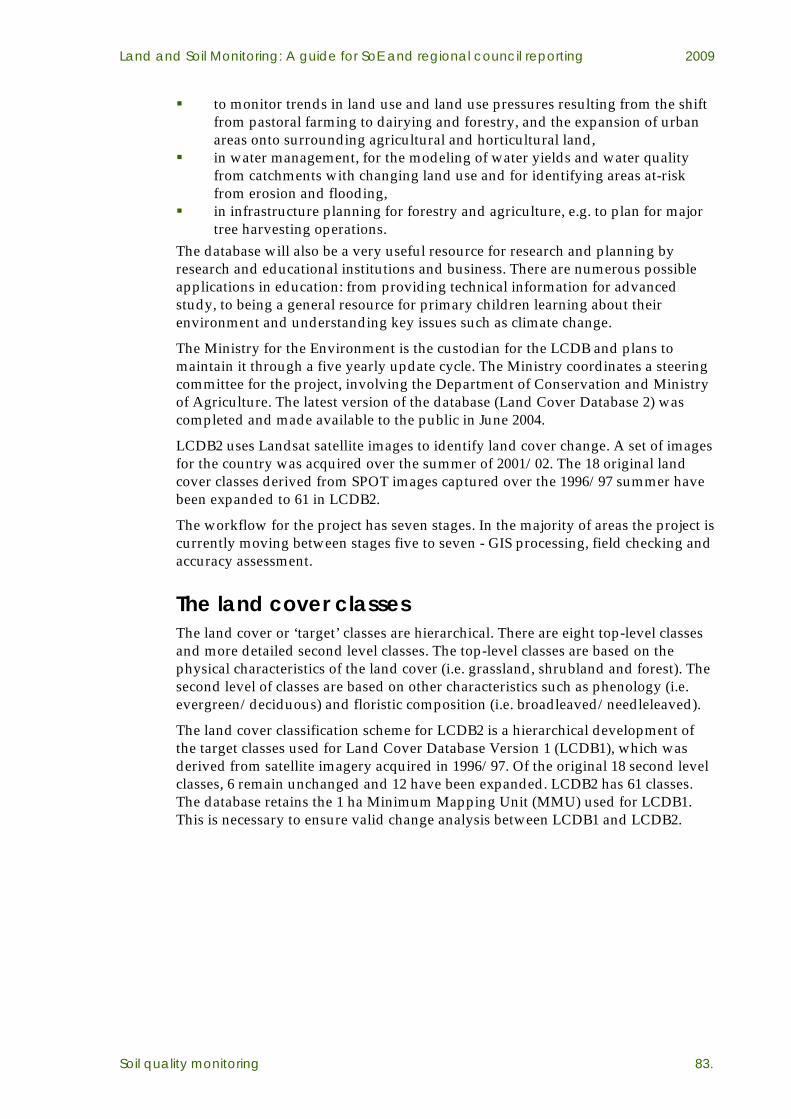
Land and Soil Monitoring: A guide for SoE and regional council reporting 2009
Soil quality monitoring 83.
to monitor trends in land use and land use pressures resulting from the shift from pastoral farming to dairying and forestry, and the expansion of urban areas onto surrounding agricultural and horticultural land,
in water management, for the modeling of water yields and water quality from catchments with changing land use and for identifying areas at-risk from erosion and flooding,
in infrastructure planning for forestry and agriculture, e.g. to plan for major tree harvesting operations.
The database will also be a very useful resource for research and planning by research and educational institutions and business. There are numerous possible applications in education: from providing technical information for advanced study, to being a general resource for primary children learning about their environment and understanding key issues such as climate change.
The Ministry for the Environment is the custodian for the LCDB and plans to maintain it through a five yearly update cycle. The Ministry coordinates a steering committee for the project, involving the Department of Conservation and Ministry of Agriculture. The latest version of the database (Land Cover Database 2) was completed and made available to the public in June 2004.
LCDB2 uses Landsat satellite images to identify land cover change. A set of images for the country was acquired over the summer of 2001/02. The 18 original land cover classes derived from SPOT images captured over the 1996/97 summer have been expanded to 61 in LCDB2.
The workflow for the project has seven stages. In the majority of areas the project is currently moving between stages five to seven - GIS processing, field checking and accuracy assessment.
The land cover classes The land cover or ‘target’ classes are hierarchical. There are eight top-level classes and more detailed second level classes. The top-level classes are based on the physical characteristics of the land cover (i.e. grassland, shrubland and forest). The second level of classes are based on other characteristics such as phenology (i.e. evergreen/deciduous) and floristic composition (i.e. broadleaved/needleleaved).
The land cover classification scheme for LCDB2 is a hierarchical development of the target classes used for Land Cover Database Version 1 (LCDB1), which was derived from satellite imagery acquired in 1996/97. Of the original 18 second level classes, 6 remain unchanged and 12 have been expanded. LCDB2 has 61 classes. The database retains the 1 ha Minimum Mapping Unit (MMU) used for LCDB1. This is necessary to ensure valid change analysis between LCDB1 and LCDB2.

Land and Soil Monitoring: A guide for SoE and regional council reporting 2009
Soil quality monitoring 84.
Target Classes for Land Cover Database Version 2
Ist Order Class LCDB1 Class LCDB2 Class
1 Urban area 1 Built-up area
2 Urban open space 2 Urban parkland
3 Surface mine
4 Dump
Artificial surfaces 3 Mines and dumps
5 Rural infrastructure
4 Coastal sand 10 Coastal sand and gravel
11 River and lakeshore gravel and rock
12 Landslide
13 Alpine gravel and rock
14 Permanent snow and ice
Bare or lightly vegetated surfaces
5 Bare ground
15 Alpine grass/herbfield
20 Lake and pond
21 River Water bodies
6 Inland water
22 Estuarine open water
30 Short-rotation cropland
31 Vineyard Cropland
9 Primary horticulture
32 Orchard and other perennial crops
40 High-producing exotic grassland
10 Primarily pastoral
41 Low-producing exotic grassland
42 Short tussock grassland
43 Tall tussock grassland
Grassland 11 Tussock grassland
44 Depleted tussock grassland
Sedgeland 7 Inland wetland 45 Freshwater sedgeland/rushland
46 Saltmarsh Saltmarsh
8 Coastal wetland
47 Flaxland
50 Bracken fern
51 Gorse and broom
52 Manuka/kanuka
53 Matagouri
54 Broadleaved indigenous hardwoods
55 Sub-alpine shrubland
Scrub and/or shrubland
12 Scrub
56 Mixed exotic shrubland

Land and Soil Monitoring: A guide for SoE and regional council reporting 2009
Soil quality monitoring 85.
57 Grey scrub
13 Mangroves 60 Mangrove
14 Major shelterbelts 61 Major shelterbelts
62 Afforestation (not imaged)
63 Afforestation (imaged post LCDB 1)
64 Pine forest – harvested
65 Pine forest – open canopy
66 Pine forest – closed canopy
15 Planted forest
67 Other exotic forest
16 Willows and poplars 68 Deciduous hardwoods
Forest
17 Indigenous forest 69a to 69u
Indigenous forest classes from FSMS 6 (18 in total)
Unclassified 18 Unclassified 70 Unclassified
For further information see www.mfe.govt.nz/issues/land/land-cover-dbase.html

Land and Soil Monitoring: A guide for SoE and regional council reporting 2009
Soil quality monitoring 86.
References Aichberger, K. and Bäck, J. (2001). The Austrian soil sampling procedure tested in a
field study (CEEM-project). The Science of The Total Environment, 264 (1-2), 8 January 2001, pp 175-180.
Blakemore L.C., Searle P.L. and Daly B.K (1987). Methods for chemical analysis of soils. NZ Soil Bureau Scientific Report 80, Lower Hutt, DSIR Soil Bureau.
Bremner, J.M. (1965). Organic nitrogen in soils. In W.V. Bartholomew and F.E. Clark (eds.) Soil nitrogen. Agron. Monogr. 10. ASA, Madison, WI. pp. 93–132.
Brookes, P.C, Powlson, D.S and Jenkinson, D.S (1982). Measurement of microbial biomass phosphorus in soil. Soil Biology and Biochemistry 14, 319-329.
Carter, M.R., Gregorich, E.G., Anderson, D.W., Doran, J.W., Janzen, H.H., Pierce, F.J. (1997). Concepts of soil quality and their significance. In Soil Quality for Crop Production and Ecosystem Health, Gregorich E.G., Carter, M.R. Eds.; Elsevier: Amsterdam: 1-19.
Clayden, B. and Hewitt, A. E. (1989). Horizon notation for New Zealand soil. Division of Land and Soil Sciences, Lower Hutt.
Claydon, J.J. (1989). Determination of particle size distribution in fine grinded soils - pipette method. Division of Land and Soil Sciences Technical Record LH5. DSIR, Lincoln.
Cornforth, I.S. (1999). Selecting indicators for assessing sustainable land management. Journal of Environmental Management, 56, 173-179.
Cowling, J.C., Speir, T.W. and Percival, H.J. (1987). Potential problems with the determination of Olsen and Microbial P of soils due to the instability of 0.5M sodium bicarbonate. Communications in Soil Science and Plant Analysis. 18 (6), pp 637-652.
Doran, J.W., Coleman, D.C., Bezdicek, D.F., Stewart, B.A. Eds. (1994). Defining Soil Quality for a Sustainable Environment: SSSA Special Publication Vol. 35; Soil Science Society of America: Madison: Wisconsin, 244 pp.
Elrick, D.E. and Tanner, C.B. (1955). Influence of Sample pretreatment on soil moisture retention. Soil Science Society of America Proc. 19: 279 - 282.
Haynes, R. J. and Tregurtha, R. (1999). Effects of increasing periods under intensive arable vegetable production on biological, chemical and physical indices of soil quality. Biology & Fertility of Soils 28, 259-266.
Hewitt, A. E. (1998). New Zealand Soil Classification 2nd Edition, Manaaki Whenua Landcare Research, Lincoln.
Hill, R.B., Sparling, G., Frampton, C., Cuff, J. (2003). National Soil Quality Review and Programme Design. Technical Paper 75, Land. Ministry for the Environment, Wellington.
Giltrap, D. J. and Hewitt, A. E. (2004). Spatial variability of soil quality indicators in New Zealand soils and land uses. New Zealand Journal of Agricultural Research, 47, pp. 167-177.

Land and Soil Monitoring: A guide for SoE and regional council reporting 2009
Soil quality monitoring 87.
Gradwell, M.W. (1972). Methods for Physical Analysis of Soils in "New Zealand Soil Bureau Scientific Report 10C". Department of Scientific and Industrial Research, New Zealand.
Gradwell, M.W., and K.S. Birrell. (1979). Methods for physical analysis of soils. New Zealand Soil Bureau Sci. Rep. 10C. Dep. of Sci. and Ind. Res., Lower Hutt, New Zealand.
Kamprath, E.J. and Watson, M.E. (1980). Conventional soil and tissue tests for assessing the phosphorus status of soils. In F.E. Khasawneh et al. (eds.) The role of phosphorus in agriculture. ASA, CSSA, and SSSA. Madison, WI. pp. 433–469.
Karlen, D.L., Mausbach, M.J., Doran, J.W., Cline, R.G., Harris, R.F., Schuman, G.E. (1997). Soil Quality: A concept, definition, and framework for evaluation (A guest editorial). Soil Science Society of America Journal, 61, pp. 4-10.
Keeney, D.R. (1982). Nitrogen - availability indicies. In: Page, A.L. (ed). Methods of soil and plant analysis - Part 2 chemical and microbiological properties. 2nd edition. American Society of Agronomy, Madison, Wisconsin. Pp. 711-735.
Klute, A. (1986). Water Retention: Laboratory methods. Methods of Soil Analysis Part 1. Agronomy, No 9, American Society of Agronomy, Madison, Wisconsin. Pp 635 – 662.
Larson, W.E. and Pierce, F.J. (1994). The dynamics of soil quality as a measure of sustainable management. In Defining Soil Quality for a Sustainable Environment; Doran, J.W., Coleman, D.C., Bezdicek, D.F., Stewart, B.A., Eds.; SSSA Special Publication No 35, 37-51; Soil Science Society of America: Madison, WI.
Leco Corp. (1994). Leco Corp. (analytical instrument manufacturer). Advanced Materials and Processes. 145(6) (June 1994). pp. 42 (1).
Mackay, A.D., Simcock, R., Sparling, G.P., Vogler, I., Francis, G. (2006). Macroporosity. Internal SLURI report. AgResearch, Hamilton.
McLean, E.O. and Watson, M.E. (1985). Soil measurements of plant-available potassium. In. R.D. Munson. (ed.) Potassium in agriculture. ASA, CSSA, and SSSA, Madison, WI. pp. 277–308.
McQueen, D.J. (1993). Glossary of Soil Physical Terms. Landcare Research New Zealand Ltd.
Milne, D., Clayden, B., Singleton, P. L., Wilson, A. D. (1995). Soil description handbook (Revised Edition), Manaaki Whenua Press, Lincoln.
Murphy, J. and Riley, J. (1962). A modified single solution method for the determination of phosphate in natural waters. Anal Chim Acta 27:31–36.
Olsen, S., Cole, C., Watanabe, F., Dean, L. (1954). Estimation of available phosphorus in soils by extraction with sodium bicarbonate. USDA Circular Nr 939, US Gov. Print Office, Washington, D.C.
Olsen, S.R. and Sommers, L.E. (1982). Phosphorus. In: Page, A.L. et. al. (eds). Methods of Soil Analysis, Part 2, 2nd edn, Agron Monogr 9. ASA and ASSA, Madison WI, pp 403–430.
Parshotam, A. and Hewitt, A. E. (1995). Application of the Rothamsted carbon turnover model to soils in degraded semi-arid land in New Zealand. Environment International 21, 693-697.

Land and Soil Monitoring: A guide for SoE and regional council reporting 2009
Soil quality monitoring 88.
Resource Management Act 1991. Wellington, New Zealand Government Printer.
Shen, S.M., Brookes, P.C., Jenkinson, D.S. (1987). Soil respiration and measurement of microbial biomass C by the fumigation technique in fresh and air-dried soil. Soil Biol Biochem 19:153 – 158.
Singer, M.J. and Ewing, S. (1999). Soil Quality. In Interdisciplinary aspects of soil science, Section 11 Handbook of Soil Science; (Sumner, Malcolm.E. Ed.); CRC Press: New York,: 272-298.
Sojka, R.E. and Upchurch, D.R. (1999). Reservations regarding the soil quality concept. Soil Science Society of America Journal, 63 (5), 1039-1054.
Sparling, G.S., Rijkse, W., Wilde, H., van der Weerden, T. J., Beare, M. H., Francis, G. S. (2000). Implementing soil quality indicators for land: Research Report for 1998/1999. Landcare Research Contract Report: 9900/108, Hamilton, Landcare Research.
Sparling, G. P., Rijkse, W., Wilde, R. H., van der Weerden, T., Beare, M. H., Francis, G. S. (2001). Implementing soil quality indicators for land. Research report for 2000-2001 and Final Report for MfE Project Number 5089. Landcare Research Contract Report: LC0102/015, Hamilton, Landcare Research.

Chapter 4
Assessing soil stability
Authors: A.S. Burton, A. Taylor and D. L. Hicks.

Land and Soil Monitoring: A guide for SoE and regional council reporting 2009
Assessing soil stability 90.

Land and Soil Monitoring: A guide for SoE and regional council reporting 2009
Assessing soil stability 91.
Contents
1 Introduction.......................................................................................93
1.1 Definitions of indicators..................................................................................................... 93
1.1.1 Soil stability ................................................................................................................... 93 1.1.2 Soil disturbance............................................................................................................. 94 1.1.3 Soil intactness ................................................................................................................ 94 1.1.4 Soil quality ..................................................................................................................... 94
1.2 Point sample analysis ......................................................................................................... 94
2 Survey design....................................................................................95
2.1 Measurement from aerial photographs ........................................................................... 95
2.1.1 Selecting photography ................................................................................................. 95 2.1.2 Interpreting photos....................................................................................................... 96 2.1.3 Viewing scale................................................................................................................. 96
2.2 A point sample on a topographic map grid .................................................................... 96
2.2.1 Determining sample size ............................................................................................. 96 2.2.2 Locating sample points ................................................................................................ 97
3 Recording data.................................................................................98
3.1 Point identification number............................................................................................... 99
3.2 Grid reference ...................................................................................................................... 99
3.3 Land use ............................................................................................................................... 99
3.4 Secondary vegetation ....................................................................................................... 102
3.5 Land stability ..................................................................................................................... 102
3.6 Nature of disturbance....................................................................................................... 103
3.7 Landform............................................................................................................................ 104
3.8 Bare soil .............................................................................................................................. 105
4 Storing data.....................................................................................106
4.1 Recording data from conventional aerial photographs (contacts or enlargements)106
4.2 Recording data from orthophotos .................................................................................. 106
4.3 Editing data........................................................................................................................ 106
4.4 Storing repeat data............................................................................................................ 106
5 Data analysis...................................................................................107
5.1 Data processing methods................................................................................................. 107
5.1.1 Manual count .............................................................................................................. 107 5.1.2 Pivot table .................................................................................................................... 107 5.1.3 Spreadsheet analysis .................................................................................................. 107
5.2 Types of analysis ............................................................................................................... 107
5.3 Summary tables................................................................................................................. 108

Land and Soil Monitoring: A guide for SoE and regional council reporting 2009
Assessing soil stability 92.
6 Statistical interpretation .................................................................108
6.1 Photo interpretation error................................................................................................ 108
6.2 Sampling error................................................................................................................... 108
6.3 Precision of measurements .............................................................................................. 109
6.3.1 Point counts ................................................................................................................. 109 6.3.2 Cluster samples........................................................................................................... 110
6.4 Sample representativeness............................................................................................... 110
6.4.1 Point counts ................................................................................................................. 110 6.4.2 Cluster samples........................................................................................................... 110
6.5 Tests for significance of comparisons............................................................................. 111
6.5.1 Test that proportions in the same class for two samples are significantly different on the same date ......................................................................................................... 111 6.5.2 Test that the proportion of a sample falling into a particular class has changed significantly between two dates ............................................................................... 112 6.5.3 Cautionary note .......................................................................................................... 112
6.6 Extracting sub-sets from regional data .......................................................................... 113
6.6.1 Cautionary note .......................................................................................................... 113 7 Documents, their use and environmental interpretation ............113
7.1 Standard reports................................................................................................................ 114
7.2 Report contents and focus ............................................................................................... 114
8 References ......................................................................................115

Land and Soil Monitoring: A guide for SoE and regional council reporting 2009
Assessing soil stability 93.
1 Introduction The objective of this chapter is to provide a procedure for assessing soil stability, soil intactness and soil disturbance, and their change over time. A procedure is needed because councils have a statutory responsibility to collect information about the state of the environment for their regions (Section 35, Resource Management Act). How well soil is being kept in place as a resource for farming, forestry and conservation; and how much soil is being lost through erosion, deposition, or land use-related disturbance, are necessary components of a good State of the Environment (SoE) report. Since the Act was passed in 1991, councils have trialed different ways to monitor soil, so the measures and techniques have developed over time. The method outlined in this chapter has been previously known as soil erosion, soil stability, soil intactness or soil disturbance monitoring, depending on each council’s focus. Its inclusion in the LMF Land and Soil Monitoring guidelines is intended to provide a standard procedure, with clear descriptions of the components that are reported as indicators and how to measure them, while allowing councils sufficient flexibility to focus on components relevant to their regions. The procedure has mainly been applied at a regional scale, to obtain information about soil for SoE reports. Councils have often found additional uses for the data, such as summaries of land use; details about vegetation associated with different land uses; assessing the extent of vegetative soil conservation measures; or sourcing facts and figures for various policy documents and publications. Some councils have also applied the procedure at a detailed scale, to monitor catchments or management zones. This chapter has been written with these uses in mind also.
1.1 Definitions of indicators 1.1.1 Soil stability
Characterises whether soil is: stable; unstable but inactive (erosion-prone); recently eroded; freshly eroding.
It provides an assessment of soil’s susceptibility to disturbance by natural processes, past and present, as well as a framework for assessing disturbance by land use. The assessment relates to soil, not to underlying weathered regolith or unweathered rock. Between 1998 and 2008, several point sample survey reports used the term “soil state” to denote soil stability. “Soil state” might be interpreted as encompassing other assessments such as soil structure, fertility or biological activity. This manual substitutes soil stability to clarify what this chapter’s point sample procedure is designed to assess.

Land and Soil Monitoring: A guide for SoE and regional council reporting 2009
Assessing soil stability 94.
1.1.2 Soil disturbance Relates to whether soil is currently at risk of removal or re-position, either through natural processes (erosion, deposition) or land use-related activities (cultivation, vegetation clearance, earthworks). Soil disturbance manifests itself as: decrease in thickness; increase in exposed area; movement of soil on-site; or removal of soil off-site.
The disturbance may reduce land's productive capacity on-site. Off-site, it may create environmental pressures, notably if soil enters water bodies. The procedure described in this chapter uses change in exposed area as an indicator.
1.1.3 Soil intactness Expresses whether soil is currently staying in place. A decrease in soil intactness occurs when soil is disturbed, either by natural processes or by land use. Soil intactness manifests itself as the inverse of soil disturbance i.e. increase in thickness; decrease in exposed area; no movement of soil on-site; or no removal of soil off-site.
The procedure described in this chapter uses change in vegetated area as an indicator.
1.1.4 Soil quality There are other ways for soil to decline, notably: break-down of structure by machine compaction or animal treading; loss of nutrients by removal of produce, leaching to groundwater, or
volatilisation to the atmosphere; and decrease in topsoil depth by oxidation of organic matter, combustion or
shrinkage after draining. These declines are commonly thought of as changes in a soil's condition, quality or health. They cannot be assessed through the point sample analysis technique described in this chapter. The soil quality monitoring chapter should be followed instead.
1.2 Point sample analysis Point sample analysis is a statistical technique that has long been applied in the natural sciences, to extract sample data from field sites, aerial photographs, or maps. The particular technique described in this chapter, has been designed to ascertain soil stability, intactness and disturbance.

Land and Soil Monitoring: A guide for SoE and regional council reporting 2009
Assessing soil stability 95.
The technique was devised by Dr Douglas Hicks of Ecological Research Associates, and has been refined progressively since its inception in 1998. To date it has been used by eight regional councils and unitary authorities. Reports relating to each survey are listed in Section 8: References. Other techniques were trialed by councils prior to and during this period, following the Ministry for Environment’s recommendations (Williams and Mulcock, 1996). A review commissioned by the Ministry (Lambrechtsen and Hicks, 2001) outlines the different monitoring techniques and their use under New Zealand conditions. It was completed to assist local government in the development and choice of techniques for regional soil erosion monitoring programmes. The Land Monitoring Forum (LMF) recognises the point sample analysis technique as most suitable for monitoring soil stability, intactness and disturbance at a catchment and regional scale. Combined with other monitoring techniques it will have value for monitoring at a national scale. It meets most requirements of local and central government for SoE reporting, being: suitable for all land uses, including urban; hierarchical i.e. finer sub-divisions allow more detail at regional and
catchment levels; simple, robust, easily understood, and easily repeated; and relatively cheap and quick.
2 Survey design Key features of survey design are measurement from aerial photographs, and a point sample located on a topographic map grid.
2.1 Measurement from aerial photographs The reasons for selecting this technique are: Digital aerial photographs are now available for all parts of New Zealand. They enable a region-wide sample to be collected faster than by field
measurement at sample points. A region-wide sample enables firm identification of where soil disturbance
occurs. Current land use and associated vegetation can also be recorded from the
aerial photos.
2.1.1 Selecting photography Assessments are presently carried out using aerial photography, though satellite images may be used in the foreseeable future. As the assessment is a “snapshot” in time the complete survey area should be photographed in a compact time period (preferably within twelve months). Photographs need to be clear enough to allow accurate assessment. A pixel size no greater than 1 metre is recommended. This will allow effective identification of landscape characteristics, down to a viewing scale of 1:2,500. If a point sample analysis is to be used for region-wide SoE reporting, photography of the survey area should be orthorectified and stored in a geographic information

Land and Soil Monitoring: A guide for SoE and regional council reporting 2009
Assessing soil stability 96.
system (GIS), to enable accurate geo-referencing of sample points. However point analysis may also be applied to unrectified aerial photographs. This would be useful for special purpose investigations at catchment scale, where comparisons with historic photography are sometimes needed.
2.1.2 Interpreting photos The analyst carrying out the survey needs advanced photo-interpretation and basic GIS and database management skills. The assessment procedure adopted for recently completed regional surveys uses on-screen aerial photo interpretation within a GIS framework. This allows keyboard data entry into a database while photographic interpretation is carried out. It also allows the referencing of other available data layers such as vegetation surveys, digital terrain models and previous survey information. Earlier surveys (both regional and catchment) entailed point sampling from contact prints or enlargements of aerial photographs. This can still be done using the procedure described in this chapter; but requires greater time for the manual location of points (map grid intersections) on the prints/enlargements; also for subsequent data entry from recording sheets.
2.1.3 Viewing scale The point sample analysis should be carried out at a viewing scale of 1:10 000 or greater. This is a minimum scale for good photo-interpretation of landscape data. If using orthophotographs in a GIS, the observer may zoom to larger scales to inspect detail at points when necessary, and to smaller scales to view points in the context of surrounding terrain. Measurements may be made at any scale between 1:10,000 and 1 :2,500.
2.2 A point sample on a topographic map grid Reasons for selecting this strategy are : Orthophoto coverage is amenable to direct overlay of one of the topographic
map grids; New Zealand Map Grid (NZMG) or New Zealand Transverse Mercator (NZTM).
The map grid, although spatially non-random, provides a random sample of the underlying terrain, because soils and land uses are irregularly distributed in geographic space
Spacing can be varied e.g. 1 km by 1km for smaller regions, 3 km by 3 km for larger, providing sufficient points to represent region-wide figures.
Points on a map grid, stored in a council's geographic information system (GIS), can be easily relocated for resurvey.
2.2.1 Determining sample size Sampling density is determined by the area to be sampled, divided by the number of points needed to obtain the required error margin. For region-wide sampling it is expressed as square kilometres per point. For catchment-scale sampling, it is expressed as points per square kilometre.

Land and Soil Monitoring: A guide for SoE and regional council reporting 2009
Assessing soil stability 97.
The number of points needed can be determined by deciding on an acceptable margin of error. Statistical sampling theory is used to work out the required sample size. Kolmogorov’s formula provides a preliminary estimate :
n = (1.36/e)2
where n is sample size and e is maximum divergence between sample and population distributions.
For instance, n = 1000 randomly located points would provide a sample size that estimates a distribution (for any parameter e.g. bare soil) to within e = +-4.3% of the true distribution at the 95% confidence level.
Table 4.1: Error margins (at 95% confidence) associated with point count estimates for various sample sizes.
Sample size (n) Error margins (e)
100 13.6%
250 8.6%
500 6.1%
1000 4.3%
2500 2.7%
5000 1.9%
10000 1.4%
In regional point sample surveys to date, calculated error margins for most data items have been considerably better than Kolmogorov’s formula suggests. Provided a regional point total exceeds about 2000, past experience suggests the following sample error margins (+- 2 standard errors at 95% confidence) are practical targets: 1.0% for point counts (proportion containing intact or disturbed soil), 0.1% for cluster measurements (area of vegetated or bare soil).
There will always be instances where a target error margin is exceeded for identifiable reasons (see Section 6.2 : Sampling Error). This need not be a concern so long as most data items fall within the target range.
2.2.2 Locating sample points Sample points are surrounded by a defined area in which land characteristics are assessed. Consideration of the defined area’s characteristics is important because data recorded at an exact point, or a small area around a point, will often be misleading. For example, if a point happens to be on a pine tree in the middle of a grassed paddock it should be recorded as pasture with scattered trees, not as pine forest. If a point lies on grass in a paddock that is a mix of pasture with scattered trees, it should not be recorded as clean pasture. Only recording erosion when bare ground lies exactly under each point, would result in under-recording of the erosion’s extent. To overcome these and similar issues, the sampling area is delineated by one hectare centered on each point. A square shape (Figure 4.1) facilitates measuring areas or percentages, using a dot grid superimposed on the photograph.

Land and Soil Monitoring: A guide for SoE and regional council reporting 2009
Assessing soil stability 98.
At some points, land use boundaries will be encountered within the one hectare area. In this situation there are two options. The first is to record whichever land use occupies the greater area, then record the lesser land use as associated vegetation. An alternative is to drag the one-hectare square sideways or up and down until it is on a single land use. This option enables any secondary vegetation associated with the greater land use to be recorded, but has the disadvantage that it departs from the random sampling properties of a regular grid. A map grid is the most suitable tool for placing sample points. Regional point sample surveys carried out to date have used either the New Zealand Map Grid or its recent replacement the New Zealand Transverse Mercator Grid. Sampling points have been established on these grids at the grid intersections. Spacings at 1km by 1km through to 3km by 3km have been used depending on the number of points required. GIS procedures can generate points and squares at the corresponding spacing. They are a quick way to provide the required number of points for the survey area, and make it easy to relocate sample points for resurveying.
Figure 4.1: NZMS 260 topographic map sheet grid with 1 hectare square sample points centred on each 2km intersection overlaying an orthophoto.
3 Recording data The following attributes form a core data set for reporting soil intactness, when a region-wide point sample is undertaken for SoE reporting. Some variation in detail may be required for different regions’ surveys and can be accommodated, provided the data can be aggregated back to the core data set as described below. For example, it may be important to record avocado orchards separately from other orchards where the former are regionally significant e.g. Bay of Plenty. The core data set is mostly recorded as single-letter alphabetic codes. This feature has the following advantages : quick data entry; easy sorting; word labels can be substituted for single letters, if need be; and codes can be sub-divided by adding an extra letter or character e.g. asterix.
Three exceptions to alphabetic coding are : the recording of percentage bare soil as an integer number (1 to 100);
Land and Soil Monitoring: A guide for SoE and regional council reporting 2009
Assessing soil stability 99.
computer generation of a point identification number; and a matching eight-digit map grid reference.
Additional data recording codes (or subdivisions of existing codes) are usually needed when undertaking a special purpose point sample e.g. extent or condition of soil conservation measures within a catchment. The capacity to accommodate extra user-defined codes adds flexibility to the standard data recording method described in this chapter. The only requirements when adding these, are to : define them, avoid using a code that already denotes something else, ensure that additional codes can be aggregated back to the core data set.
3.1 Point identification number A unique reference number for each sample point, from 1 to x is recorded. This is required for sample data checks and useful when querying the database for points with specific features.
3.2 Grid reference Use the New Zealand Map Grid for an existing survey, or the New Zealand Transverse Mercator for a new one. The means of adjusting from one reference system to the other will be simple. Record the grid reference to four digits easting and four digits northing. This is essential if the same points are to be located for a future re-survey. It also enables point data to be analysed relative to other spatial data stored in the GIS; for instance the Land Cover Database or Land Resource Inventory. A GIS can generate grid references automatically; but if point sampling is performed manually from old photographs, it becomes necessary to identify points on, and read grid references off, a printed map.
3.3 Land use The land use categories chosen will depend on the level of information required from the survey. For example, where horticulture is widespread in a district or catchment it may be beneficial to differentiate the various types. It is important when selecting individual categories that they can be aggregated back to the New Zealand Land Cover Database (LCDB1 or LCDB2). This is currently the most suitable system to use for national monitoring. The following land use categories have been used as a base set for a number of completed surveys, and should be used as a minimum data set for future surveys. They are readily aggregated back or matched directly to the class sets of LCDB1 and 2. (See Chapter 3: Appendix IV).
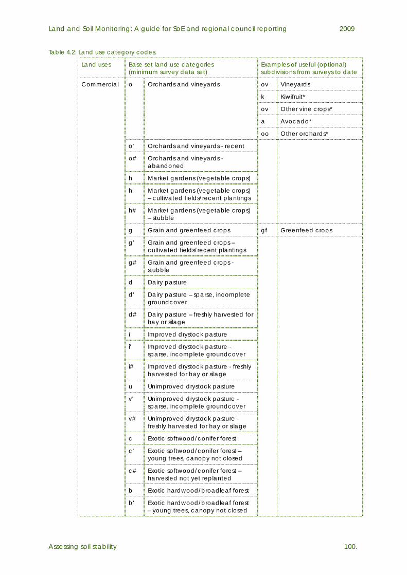
Land and Soil Monitoring: A guide for SoE and regional council reporting 2009
Assessing soil stability 100.
Table 4.2: Land use category codes.
Land uses Base set land use categories (minimum survey data set)
Examples of useful (optional) subdivisions from surveys to date
ov Vineyards
k Kiwifruit*
ov Other vine crops*
a Avocado*
o Orchards and vineyards
oo Other orchards*
o' Orchards and vineyards - recent
o# Orchards and vineyards - abandoned
h Market gardens (vegetable crops)
h' Market gardens (vegetable crops) – cultivated fields/recent plantings
h# Market gardens (vegetable crops) – stubble
g Grain and greenfeed crops gf Greenfeed crops
g' Grain and greenfeed crops – cultivated fields/recent plantings
g# Grain and greenfeed crops - stubble
d Dairy pasture
d' Dairy pasture – sparse, incomplete groundcover
d# Dairy pasture – freshly harvested for hay or silage
i Improved drystock pasture
i' Improved drystock pasture - sparse, incomplete groundcover
i# Improved drystock pasture - freshly harvested for hay or silage
u Unimproved drystock pasture
v' Unimproved drystock pasture - sparse, incomplete groundcover
v# Unimproved drystock pasture -freshly harvested for hay or silage
c Exotic softwood/conifer forest
c' Exotic softwood/conifer forest – young trees, canopy not closed
c# Exotic softwood/conifer forest – harvested not yet replanted
b Exotic hardwood/broadleaf forest
Commercial
b' Exotic hardwood/broadleaf forest – young trees, canopy not closed

Land and Soil Monitoring: A guide for SoE and regional council reporting 2009
Assessing soil stability 101.
b# Exotic hardwood/broadleaf forest – harvested not yet replanted
f Native (natural) forest
f# Native (natural) forest – recently cleared
s Native (natural) scrub sf Fern scrub (bracken, crown fern, ring fern)
s# Native (natural) scrub – recently cleared
x Exotic scrub
x# Exotic scrub – recently cleared
t Tussock grass
a Alpine herbfield? sa Sub-alpine scrub
e exotic herbaceous weeds
w wetland vegetation (rushes, sedges, raupo, flax)
m coastal vegetation (sand-binding or salt-tolerant plants)
mc Native (natural) sand-binding plants
Conservation
mg Mangroves
A second set of codes is not needed for analyzing soil intactness/disturbance, but has to be used when points fall on features such as those given below. For these land uses no other attributes are normally recorded (but may be if needed by a council for some other purpose).
Table 4.3: Secondary land use codes.
Secondary land use feature codes Example of simplified coding from Tasman 2004 survey
by Farm buildings, yards, dwellings (including lifestyle homes)
bg Indoor agriculture (glasshouses, hydroponics, poultry sheds, pig sheds)
bi Industrial buildings on rural sites
bi Farm buildings, yards, rural industrial sites and irrigation ponds
qm Quarries and mines q Quarries and mines
rr Rural roads, railways and airfields r Roads, railways and airfields
uo Urban open space (parks, playing fields, waste ground)
ub Urban buildings (houses, factories, shops, public buildings)
ur Urban roads, railways and airfields
ur Urban buildings, open spaces, roads and airfields
wb Waterbodies
sl Shorelines

Land and Soil Monitoring: A guide for SoE and regional council reporting 2009
Assessing soil stability 102.
3.4 Secondary vegetation The same codes as above are used to indicate when another vegetation type is intermingled with the main land use. For example; land use = u and secondary vegetation = s denotes unimproved pasture with native scrub. To add further information to the secondary vegetation code, relating to the state of the land cover in cropland or grassland: absence of an asterix or the like denotes extensive secondary vegetation e.g. us
denotes unimproved dry stock pasture with clumps of natural scrub, a speech mark denotes scattered secondary vegetation e.g. us’, shelterbelts are denoted by an asterisk e.g. b*; hedgerows by an ampersand
e.g. b@. In scrub or forest: secondary vegetation emerging through canopy (or in canopy gaps) is
normally recorded without any suffix e.g. xs is exotic scrub with natural scrub emerging through canopy; sx is natural scrub with canopy gaps occupied by exotic scrub,
a speech mark may be used to denote sparse secondary vegetation in canopy gaps e.g. sx’ is natural scrub where canopy gaps are occupied by sparse exotic scrub (interspersed with bare soil or rock).
3.5 Land stability These codes are not essential for analysing current soil disturbance. However in surveys to date, they have been prerequisite to ascertaining the extent and timing of past disturbance.
Table 4.4: Land stability codes.
Land stability codes Description
s Stable surfaces; vegetated Show no sign of past erosion. Have a smooth appearance and are completely vegetated (unless topsoil is disturbed by land use).
u Erosion-prone, unstable surfaces; inactive, vegetated
Unstable surfaces, inactive, vegetated: show signs of past erosion but are currently not eroding. Erosion scars have healed and are well vegetated. Erosion has usually occurred at least a decade prior to photography.
r Eroded, unstable surfaces; recently disturbed, revegetating
Unstable surfaces, recently disturbed, revegetating. Erosion scars are partially vegetated, surface is still rough. Erosion feature is identifiable and has usually occurred in the decade prior to photography.
e Eroding, unstable surfaces; freshly disturbed, bare
Unstable surfaces, freshly disturbed, bare: easily identifiable erosion feature, active with much bare ground. Has usually occurred in the year prior to photography. Recording a point as eroding does not mean that 100% of the surrounding one-hectare area is eroding; it denotes erosion is occurring on soil under the land use that’s being practiced in the point’s immediate vicinity.

Land and Soil Monitoring: A guide for SoE and regional council reporting 2009
Assessing soil stability 103.
3.6 Nature of disturbance These codes are essential for noting where soil is currently disturbed. From them, stability is measured inversely i.e. where soil is currently in place. In particular, the codes differentiate between soil disturbance caused by erosion or deposition; and soil disturbance caused by land use (exposing bare soil to risk of erosion or deposition). The categories chosen will depend on the level of information required. Only two codes are required for SoE reporting but regional council surveys usually require a more detailed set of codes.
Table 4.5: Soil disturbance codes.
Core codes for SoE Reporting Suggested codes for regional council use
a Exposed by land use-related activities
c Exposed by cultivation
n Exposed by natural erosion or deposition
x Exposed by harvest
y Exposed by spraying
z Exposed by grazing
t Exposed by farm or forest track (not sealed)
d Exposed by drain excavation, cleaning or tile drainage
Topsoil
e Exposed by earthworks
l Landslide or slip
u Slump or flow
a Debris avalanche
ll Large slope failure
p Tunnel (under-runner)
g Open gully
Subsoil
lg Large gully
b Stream bank scour
s Stream bank deposition
w Wind erosion or deposition of sand
h Sheetwash and windblow scalds (excluding sand)
br Rock outcrops, rockfalls or scree deposits
Other
ge Geothermal activity
Topsoil disturbance is generally due to land use. It is recorded where visible on s and u surfaces. It is not recorded where visible on r and e surfaces, as in these cases it is associated with, and over-ridden by, subsoil or other disturbance. Subsoil and Other disturbances are generally due to natural processes, but may be exacerbated by land use. They are recorded where visible on r and e surfaces. These

Land and Soil Monitoring: A guide for SoE and regional council reporting 2009
Assessing soil stability 104.
categories can be readily aggregated back to erosion types in the NZLRI classification and may prove useful when interrogating information from both datasets.
3.7 Landform The following landforms are recorded. They are not essential for ascertaining soil disturbance, but may be useful for other analyses.
Table 4.6: Landform codes.
Core landform codes Optional additional landform codes
m Mountains (high, bare or sparsely vegetated)
m' Mountains – distinct colluvial footslopes
s Steeplands (low, densely vegetated)
s' Steeplands – distinct colluvial footslopes
h Hill country (hillsides, ridges, spurs)
h' Hill country – distinct colluvial footslopes
d Downlands, plateaux d' Downlands – distinct colluvial footslopes
t Raised terraces and plains
f Floodplains
fp Protected floodplains
w Wetlands
wd Drained wetlands
u Active sand dunes (bare)
ur Old dune ridges (vegetated)
uf Old dune flats (vegetated)
tc Raised coastal terraces
fc Coastal flats
Additional landform codes need to be used at points which lack soil. For these landforms no other attributes are recorded. Some of these categories can be sub-divided if extra information is required.

Land and Soil Monitoring: A guide for SoE and regional council reporting 2009
Assessing soil stability 105.
Table 4.7: Landform codes for points lacking soil.
Landform codes Example of code subdivision from EBOP 2005 survey
l Lake
p Pond
la Large river (alluvial)
a Small river or stream
a River or stream
ls Large river (rock channel)
e Estuary
b Beach
r Intertidal rock platform
c Cliff/bluff/gorge
d Dune
3.8 Bare soil The measurement of bare soil was not undertaken in early surveys but is now an essential part of the survey method. Bare soil due to land use is recorded for s and u surfaces. The convention is not to record it for r or e surfaces, where it may be present but is over-ridden by bare soil attributed to natural disturbance. Bare soil due to natural processes is recorded for e surfaces. The convention is not to record it for r surfaces, where it may be present but is diffuse amongst revegetation. Cluster sampling is used to measure the percentage of bare soil. It entails recording the incidence of bare soil at each of 100 dots set in a 10 x 10 grid within a one hectare area around the sample point. The number of dots with bare soil is recorded as an attribute.
Figure 4.2: Cluster sample of 100 dots around a sample point.

Land and Soil Monitoring: A guide for SoE and regional council reporting 2009
Assessing soil stability 106.
4 Storing data In recently completed surveys, sample point locations have been stored in a GIS map layer. These are cross-referenced to a GIS attribute table which contains the raw data. Any GIS software can be used provided that the data is saved in a delimited format. In this format data can be readily exported to spreadsheet programmes (such as Excel) and other statistical analysis tools. This facilitates future access and re-analysis.
4.1 Recording data from conventional aerial photographs (contacts or enlargements) Manually record data on a check-sheet next to the contact or enlargement. It is quicker to do this and then subsequently enter the data into a computer, than to constantly turn back and forth between the contact print (viewed through a magnifier or stereoscope) or enlargement (viewed by eye on a desk-top) and a computer on another desk.
4.2 Recording data from orthophotos Key data into a point-linked menu which is displayed on-screen next to the point and then store it in a GIS attribute table. Standard GIS procedures exist for setting up menus and attribute tables. Advantages of storing data in an attribute table include the ability to: query tables to find points where no data have been recorded or data have
been incorrectly recorded; and export tables to spreadsheets for subsequent editing and analysis.
4.3 Editing data Codes used to record data can be altered once they are entered into spreadsheets by using “find and replace” facilities. These facilities can be useful for: correcting data that have been wrongly coded; adding extra codes (after overlaying other GIS data layers or cross-referencing
to printed maps); and codifying comments (which are annotated on checksheets or in attribute
tables).
4.4 Storing repeat data In the event that a point sample is repeated, it is best to store new data in a separate attribute table, identical in structure to the original. This avoids the risk of accidentally overwriting data from the original survey. Copy the new and original

Land and Soil Monitoring: A guide for SoE and regional council reporting 2009
Assessing soil stability 107.
attribute tables into separate spreadsheets. After checking and correcting new data, copy the relevant columns from both spreadsheets into a separate, larger spreadsheet for comparison. Always copy and cross-check either the point number or the grid reference columns from both tables. These precautions avoid operating directly on either of the attribute tables during data analysis. Copying columns from one to the other would risk mismatches, which are hard to detect and difficult to rectify.
5 Data analysis
5.1 Data processing methods There are three options; manual count, pivot table or spreadsheet analysis. Deciding which to use depends on individual preference and available time.
5.1.1 Manual count A sorted spreadsheet can be printed for each combination of codes e.g. all e (freshly eroding points) on Us (unimproved pasture with extensive scrub cover). Points can then be manually counted and summary statistics (e.g. proportions, percentages and error margins) calculated by keying point totals into a small spreadsheet that contains appropriate formulae. It is a time consuming procedure.
5.1.2 Pivot table Pivot tables can be generated from Microsoft Excel, to obtain counts for each combination of codes. It is quicker than the manual count method but complicated. Point totals still need to be transferred to a customised spreadsheet (or software package) to obtain statistics.
5.1.3 Spreadsheet analysis “Sort” and “count” operations can be used in a spreadsheet program such as Apple Works or Microsoft Excel. This method is just as quick but less complicated than the pivot table method. Data for any particular combination of codes are copied into extra columns in an analysis spreadsheet, which is set up for calculating summary statistics. Some adjustments to spreadsheet formats have been needed for each survey, to match individual councils’ requirements for data analysis and presentation. The alternative would be data transfer to a standard statistical package such as SAS. However, using a statistical package might well take longer than analysing the data in a “customised” spreadsheet.
5.2 Types of analysis For regional SoE reporting, point counts are expressed as percentages of the region wide sample, for: land stability; soil disturbance;

Land and Soil Monitoring: A guide for SoE and regional council reporting 2009
Assessing soil stability 108.
type of disturbance; and bare soil by type of disturbance.
The analysis may be (and usually is) repeated for each land use in the region. Additional analyses, not essential for SoE reporting (though often requested), can be completed for vegetation (composition/condition), and soil conservation measures. For vegetation, point counts are expressed as percentages of each land use, for: primary vegetation (sparse, dense, harvested); and associated secondary vegetation (type; whether scattered or extensive).
For soil conservation measures, point counts are expressed as percentages of stable and unstable land under each use, for: vegetative soil conservation cover (absent, scattered or extensive)
and as percentages of land under each soil conservation cover for: bare soil.
5.3 Summary tables Regardless of the chosen data processing method, its results are entered into a final set of spreadsheets. These are used to print summary tables for inclusion in reports. Their format is amenable to graph generation. Graphs are not normally included in reports (see Section 7. Documents, their use and environmental interpretation), though several surveys have graphed key statistics from the tables, for inclusion in councils’ SoE publications. Some council staff have subsequently used the tables to generate their own customised graphs for internal use or external publicatio
6 Statistical interpretation
6.1 Photo interpretation error This can be ascertained by randomly selecting 100 points and assessing them in the field. The speed of field checking can be increased by adding a filter to select points within a fixed distance from a road. These points will not be random with respect to roads, but they should still be random with respect to the recorded parameters (land use, secondary vegetation, soil stability, soil disturbance, landform). The only caveat to this is the possible influence of a road on soil disturbance and the nature of disturbance where a point lands on it or immediately next to it. For the completed surveys to date photo-interpretation accuracy has typically been in the 85% to 95% range. Most errors are simply confusion of land use etc. with another that is similar. There are few instances of completely false identification of a point as something quite unrelated.
6.2 Sampling error Point counts are expressed as percentages of the sample or sub-sample being assessed.

Land and Soil Monitoring: A guide for SoE and regional council reporting 2009
Assessing soil stability 109.
For percentages based on point counts, sample error is calculated at a 95% confidence level using the formula:
± 2 s.e. = 1.96 * sqrt (p(100-p)/n)
where:
s.e. = standard error
sqrt = square root
p = percentage from point count
n = number of points
For percentages based on cluster samples (to measure bare ground around points), sample error is calculated at a 95% confidence level using the formula:
2 s.e. = 1.96 * s/sqrt(n)
where:
s.e. = standard error
s = standard deviation of mean percentage for clusters
sqrt = square root
n = number of clusters
Sample error analysis should be carried out for all tables in the survey report, to ascertain how closely sample data match true figures for the region or catchment being surveyed. When comparing data from successive surveys, the same point sample should be used to ensure that any changes between two dates are real. No additional sampling error applies at the second date of survey (as would be the case if two different point samples were compared).
6.3 Precision of measurements Precision of measurements is calculated from the number of sample points which underpin each percentage. It is given by:
i*100/n
where:
i = Point count
n = Sample size (or sub-sample)
6.3.1 Point counts For point counts, where the soil stability in a sub-sample is calculated as a percentage of for example 100 points, the precision of calculation is +- 1%. Where it is calculated as a percentage of a lower number of points e.g. 10, the precision is +-10%. At the level of one-way splits e.g. land uses region wide, precision of measurement is very high because n is always several thousand points for the region.

Land and Soil Monitoring: A guide for SoE and regional council reporting 2009
Assessing soil stability 110.
At the level of two-way splits e.g. secondary vegetation within a land use, precision is still high provided a land use, or other parameter, is common i.e. several hundred points, but becomes low for uncommon categories i.e. less than a hundred points. Precision can become a problem for three-way splits e.g. fresh erosion amongst different categories of secondary vegetation (soil conservation cover) within a land use. Here some categories are numerous, while others are small, sometimes falling below ten points and the sampling error becomes large.
6.3.2 Cluster samples For cluster samples (measurements around a point), precision of measurement at an individual point is always +-1%, so long as the recommended 100 point measuring grid is used.
6.4 Sample representativeness Sample representativeness may be interpreted from sample error margins. Simply, a sample error margin denotes there is 95% confidence that a sample percentage for some parameter is within +/- x% of the true figure for a region. Report tables contain numerous sample error margins for different parameters, so some guidance is offered here about their interpretation.
6.4.1 Point counts High margins of error are associated with: Land uses where sample point numbers are low, because they occupy a small
percentage of the region. For example in the Auckland survey (Thompson and Hicks 2009) coastal vegetation was 0.5 percent of the region and had a sample error of+- 0.2 percent.
Primary or secondary cover components which are associated with a widespread land use but are uncommon. For example from Auckland’s (2009) survey, coastal vegetation associated with natural forest (1 point out of 383; 0.3 percent of the region; sample error +-0.5 percent). In such instances, there is certainty that the primary/secondary cover is a small component of associated vegetation, and its error margin is large relative to the percentage, simply because the percentage is so small.
6.4.2 Cluster samples High margins of error may still be attached to cluster-sampled data. Instances where error margins are in the 1 to 10% range, are caused by one or two points in a category having a percentage that greatly differs from the rest. This can occur in two situations. The first is where there are enough points to establish a statistical distribution. Here a high error margin reflects a genuine spread in the data. A typical example from Auckland’s (2009) survey: sparse primary cover under intensive uses had 51 points with bare soil and a sample error of +- 6.9 percent. Most of the points are partly covered by emerging crops, but some are freshly cultivated and still have close to 100% bare soil.

Land and Soil Monitoring: A guide for SoE and regional council reporting 2009
Assessing soil stability 111.
The second situation is where a category’s point numbers fall below 10. Here, the error margin can be wide because there are not enough points to establish a reliable statistical distribution. An example from Auckland’s (2009) survey is rank grass secondary cover in natural forest (5 points), where a single anomalous point distorts the distribution for bare soil, giving an average of 22% and an error margin of +-23.9 percent. There are simply too few points in this particular sub-sample to be confident that it indicates either the average value or the likely spread.
6.5 Tests for significance of comparisons When comparing point counts e.g. proportion of points with eroded soil under two land uses, a large number of statistical tests are available for use with enumeration statistics (numbers and proportions of observations falling into various classes). Of these, the following two are recommended on the grounds that they are: applicable to a variety of distributions, non-normal as well as normal; convenient for pairwise comparison between sub-samples; easy to calculate; and standard tests used by professional statisticians.
They will cover most situations where council staff may wish to test the significance of summary statistics before making statements about soil stability, soil disturbance, vegetation cover, or vegetation condition.
6.5.1 Test that proportions in the same class for two samples are significantly different on the same date
Example Unstable, revegetated surfaces (u) are recorded on 26 out of 30 sites in pasture with space-planted trees (Ib). The equivalent proportion for sites in pasture with scattered remnant scrub (Is’) is 19 out of 40.
p1 = 0.87 (26/30)
p2 = 0.48 (19/40)
The null hypothesis is H : p1 = p2
N1p1 + N2p2 p0 =
N1 + N2 = 0.65
p1 - p2
z = √p0(1-p0)(1/N1 + 1/N2)
= 3.39
Read z0.5a and z1-0.5a from z distribution table
Reject hypothesis if :
z < z0.5a 3.39 < -1.95 ?

Land and Soil Monitoring: A guide for SoE and regional council reporting 2009
Assessing soil stability 112.
or
z>z1-0.5a 3.39 > +1.95 ?
The null hypothesis is rejected. There is 95% confidence that the two proportions are significantly different i.e. unstable surfaces in pasture are less disturbed where trees have been space-planted compared with where remnant scrub has been left.
6.5.2 Test that the proportion of a sample falling into a particular class has changed significantly between two dates
Example Surfaces have been freshly/recently eroded on 19 out of 27 sites in pasture where remnant scrub is present. Assume that when the sites are re-surveyed in 5 years, the new proportion is 22 out of 27: Construct a contingency table
First date
In Out
Second date
In f1=16 f2=6 22
Out f3=3 f4=2 5
Total 19 8 27
p2 - p3 = f2/N - f3/N= 0 .11
se = √f2 + f3 - (f2 -f3)2/N= 0 .11
The null hypothesis is H : p2 = p3
z = p2 - p3/se = 1.00
Read z0.5a and z1-0.5a from z distribution table
Reject hypothesis if
z < z0.5a 1.00 < -1.95 ?
or
z>z1-0.5a 1.00 > +1.95 ?
The null hypothesis is not rejected. There is not 95% confidence that the changes are significant i.e. the apparent increase in erosion may be an artefact of the small sub-sample size.
6.5.3 Cautionary note In many instances council staff will not need to use these tests. Where sub-sample sizes are large and differences in proportions are substantial, values for the two sub-samples often lie outside each other’s error margins, so the conclusion is obvious. Statistical tests should be applied as a check only if there is an element of doubt. Some good rules of thumb are:

Land and Soil Monitoring: A guide for SoE and regional council reporting 2009
Assessing soil stability 113.
test a large difference in proportions if one or both sub-samples are small; and test two large sub-samples if there is a small difference in proportions.
6.6 Extracting sub-sets from regional data Data for region-wide point samples are usually stored in a council’s GIS for other uses besides SoE reporting. From a statistical viewpoint, it is safe to conduct sub-regional analyses of land use, associated vegetation, and soil stability, so long as the number of points in the subset exceeds approximately 500. Examples are local authority districts, large territorial areas, catchments, or sub-catchment management zones. Error margins for point counts and proportions will be larger than for the regional sample, typically in the 1-5% range. However changes in land use or vegetation cover between two dates are often sufficiently large to lie outside these error margins. It is safe to conduct sub-regional analyses of soil disturbance, where the number of points in a subset exceeds 100. Bare soil (disturbed) and vegetated soil (intact) are calculated from cluster samples around each point, so error margins will usually be tight, typically less than 1%. For sub-samples within a subset e.g. bare soil within a single vegetation cover associated with a land use, it is often possible to obtain a reliable percentage with a small error margin from the cluster data (bare soil), even where sub-sample size is less than 20. In this situation, one can be confident that one has a good measure of bare soil within that particular vegetation cover. However, in circumstances where for example, the sub-sample is 20 points drawn from a catchment subset of only 100 points, the error margin will be high, so one could not be confident that one has a good measure of that vegetation’s extent throughout the catchment.
6.6.1 Cautionary note In short, the point sample analysis technique has been designed to provide statistical data for regions. Region-wide samples are sufficiently large that they can also provide valid data for reasonably large subdivisions within a region. However, data analysis will not be reliable for soil intactness/disturbance in an area of land any smaller than 100 km2, or for land use/vegetation cover/soil stability in an area smaller than 500km2.
7 Documents, their use and environmental interpretation Various surveys have been completed by regional councils throughout New Zealand. Often the survey data is used for SoE reporting where the Pressure - State - Response Framework is commonly used. Not all data recorded in the survey is essential for this reporting and interpretation and reporting will vary in style depending on why and who the survey is being carried out for. It is recommended that complete surveys be viewed to gain an understanding of the data use and presentation possibilities. These are generally freely available from the councils that have carried out the surveys and are listed in the references.

Land and Soil Monitoring: A guide for SoE and regional council reporting 2009
Assessing soil stability 114.
7.1 Standard reports Up to four reports are drafted to a standard format consistent with LMF reporting requirements, then modified after review by council staff. The standard formats greatly reduce preparation time, and also ensure that data presentations are comparable amongst regions. Methods used to survey land stability and soil disturbance in the X region:
This is a record of survey procedure, and is needed to facilitate any future repeat point samples.
Land stability and soil disturbance in the X region: This is an essential council source of information for use in its regional SoE report. It contains summary statistics for land stability and soil disturbance, region-wide and by land use. When a point sample is repeated, an appendix is added to the second report, comparing current with previous results. These comparisons provide the basis for observations about change between sample dates.
Vegetation associated with land uses in the X region; and Vegetative soil conservation cover in the X region.
The latter two are useful additional documents to have, as sources of information about ancillary topics such as condition of planted cover, retention/regeneration of natural cover, planting of exotic or natural vegetation as a conservation measure, and revegetation’s impact on soil disturbance.
7.2 Report contents and focus Each report contains: An outline of the brief, and how it has been met. Presentation of point sample results as tables with brief accompanying text. Conclusions covering what the point sample shows, region-wide and for
specific land uses. Appendices including lengthier interpretations of point sample results, if
required for specific topics. The intention is to provide a readable account of why the survey has been done, and what it has found. Any discussion about what might need to be done about land use on particular soil types, or erosion under particular land uses, is avoided. That is not part of the brief for SoE reporting - though doubtless will be a subject for discussion amongst council staff once they have read a report’s contents.

Land and Soil Monitoring: A guide for SoE and regional council reporting 2009
Assessing soil stability 115.
8 References Burton, A.S. (2004). Soil Intactness Monitoring Programme for the Tasman District.
Tasman District Council. Crippen, T.F. (1999). Sand country erosion monitoring survey for the State of the
Environment Report. Report prepared for Horizons.mw. Crippen, T.F. (1999a). Hill country erosion monitoring survey for the State of the
Environment Report. Contract report for Horizons.mw. Crippen T.F., Scholes P. (2001). Gisborne Point Sampling Provisional Data Summary
and Comments. Contract report to Gisborne District Council. Crippen, T. and Hicks, D. (2004). Soil intactness assessment of the Wellington
Region. Report prepared for the Greater Wellington Regional Council. Hicks, D.L. (2000). Technical Appendices to: Rural land use on Auckland's soils; soil
erosion in Auckland's hill country; soil erosion in Auckland's sand country. Contract reports prepared for Auckland Regional Council.
Hicks, D.L. (2000a). Rural land use on Auckland’s soils. Contract report prepared for Auckland Regional Council.
Hicks, D.L. (2000b). Soil erosion in Auckland’s hill country. Contract report prepared for Auckland Regional Council.
Hicks, D.L. (2000c). Soil erosion in Auckland’s sand country. Contract report prepared for Auckland Regional Council.
Hicks, D.L. (2002). Scoping Paper: Pilot survey of map sheet T26. Contract report prepared for Wellington Regional Council.
Hicks, D.L. (2003). Soil intactness assessment of the Waikato region in 2003. Contract report prepared for Environment Waikato.
Hicks, D.L. (2005). Soil stability in the Bay of Plenty. Prepared for Environment Bay of Plenty.
Lambrechtsen, N.C. and Hicks, D.L. (2001). Soil intactness/erosion monitoring techniques: a literature review, Technical Paper 62. Ministry for the Environment.
Thompson, A. J. and Hicks, D. L. (2009). Vegetative Soil Conservation Cover in the Auckland Region 2007. Prepared for Auckland Regional Council. Auckland Regional Council Document Type TR 2009/014.
Williams, J. M. and Mulcock, C. M. (1996). National environmental indicators: building a framework for a core set. Land : review of international literature, draft framework and indicators. Agriculture New Zealand.

Land and Soil Monitoring: A guide for SoE and regional council reporting 2009
Assessing soil stability 116.
Chapter 5
Trace element monitoring
Authors: N.D Kim and M.D Taylor.

Land and Soil Monitoring: A guide for SoE and regional council reporting 2009
Trace element monitoring 118.

Land and Soil Monitoring: A guide for SoE and regional council reporting 2009
Trace element monitoring 119.
Contents 1 Introduction................................................................................... 121
2 Basic concepts and definitions ................................................... 121
2.1 Trace elements ..................................................................................................................121
2.2 Heavy metals ....................................................................................................................122
2.3 Partitioning between soils and soil pore water ...........................................................122
2.4 Interpretation of reported results ..................................................................................122
2.4.1 Conventional weight/weight units...............................................................................122 2.4.2 Utility of weight/volume units......................................................................................123 2.4.3 Checklist ............................................................................................................................123
2.5 Relationship to contaminated land investigation........................................................124
2.5.1 Contaminated land investigations.................................................................................124 2.5.2 Soil monitoring for SoE reporting..................................................................................124
3 General characteristics ............................................................... 125
3.1 Background and typical concentrations .......................................................................125
3.1.1 Definition ..........................................................................................................................125 3.1.2 Estimating background concentrations ........................................................................125
3.2 Essential and non-essential trace elements ..................................................................128
3.3 Behaviour of trace elements in soils ..............................................................................131
3.3.1 The range of chemical properties...................................................................................131 3.3.2 Dominant sorptive phases ..............................................................................................132 3.3.3 Key controls ......................................................................................................................135 3.3.4 Interactions between trace elements .............................................................................137
3.4 Sources of trace elements in productive soils ..............................................................138
3.4.1 Natural sources ................................................................................................................138 3.4.2 Anthropogenic sources ...................................................................................................139 3.4.3 Perturbation of biogeochemical cycles..........................................................................140 3.4.4 Potential issues for resource managers.........................................................................141 3.4.5 Types of guidelines..........................................................................................................142 3.4.6 Significant anthropogenic sources in New Zealand agricultural soils.....................143 3.4.7 Significant anthropogenic sources in New Zealand horticultural soils ...................147
4 Sampling for trace elements ....................................................... 148
4.1 General approach and specific recommendations ......................................................148
4.1.1 Methods of sampling.......................................................................................................148 4.1.2 Storage of fresh samples .................................................................................................149 4.1.3 Frequency of sampling....................................................................................................149 4.1.4 Time of sampling .............................................................................................................149 4.1.5 Sampling tools ..................................................................................................................149 4.1.6 Cleaning sampling equipment.......................................................................................149 4.1.7 Composition of the sampling team ...............................................................................149 4.1.8 Archiving soil samples ....................................................................................................150

Land and Soil Monitoring: A guide for SoE and regional council reporting 2009
Trace element monitoring 120.
5 Analysis.......................................................................................... 150
5.1 What trace elements could be measured? ....................................................................150
5.1.1 Common environmental suite........................................................................................150 5.1.2 Multi trace element suite.................................................................................................150
5.2 Types of extractions for measuring trace elements in soils........................................151
5.2.1 Extraction-based methods ..............................................................................................151 5.2.2 Direct methods .................................................................................................................152
5.3 Common methods of analysis for trace elements .......................................................153
5.3.1 Analysis of trace elements ..............................................................................................153 5.3.2 Quality control..................................................................................................................154
5.4 Data interpretation...........................................................................................................154
5.4.1 General comments ...........................................................................................................154 5.4.2 Interpretation of excess trace element concentrations in soils...................................155 5.4.3 Interpretation of deficiency trace element concentrations in soils............................155 5.4.4 Background assessments of trace elements published by regional councils...........157 5.4.5 Guideline values for selected trace elements in agricultural soils ............................158
6 References .................................................................................... 165

Land and Soil Monitoring: A guide for SoE and regional council reporting 2009
Trace element monitoring 121.
1 Introduction The purpose of this chapter is to provide a guide for monitoring inorganic trace elements in soils for the purposes of State of the Environment (SoE) and regional council reporting. Assessing trace elements in isolation is unwise as their behaviour is strongly influenced by other soil properties, such as pH and mineralogy. For example, iron and manganese can be considered controlling elements as they affect the chemistry of other elements. Trace organic contaminants are not specifically addressed in this chapter. However the sampling approach for persistent organic compounds (such as DDT) is usually the same as that used for trace elements. For non-persistent organic compounds, factors such as volatility and degradation after sampling need to be taken into account.
2 Basic concepts and definitions
2.1 Trace elements About 99% of the earth’s crust is composed of only ten major elements: oxygen, silicon, aluminium, iron, calcium, potassium, sodium, magnesium, titanium and phosphorus. Generally, the remaining elements in the Periodic Table are termed “trace elements”. They are usually present in the earth’s crust at concentrations of less than 100 mg/kg (parts per million). However, in some cases, the term “trace element” or “trace metal” is extended to cover five of the major metals listed above: iron, calcium, potassium, sodium and magnesium. Deficiency or excess of trace elements in soils can have a major bearing on soil health despite their low concentrations. Trace element chemistry in soils involves a range of dynamic biogeochemical processes. These may include: adsorption and desorption interactions with various solid phases; changes in oxidation states and chemical speciation; competition with other trace elements; complexation with various ligands; involvement in microbial metabolism; and uptake in plants and animals.
Some trace elements are essential micronutrients for plants and animals. Others are not. However, both essential and non-essential elements can become toxic at higher concentrations.

Land and Soil Monitoring: A guide for SoE and regional council reporting 2009
Trace element monitoring 122.
2.2 Heavy metals Heavy metals are all trace elements but their definition is imprecise. Two common definitions are: A trace element with a density greater than 6 g/cm3.
However, not all trace elements are metals in their elemental form (e.g. arsenic and selenium are non-metals) and so it can be argued that in this case the term “heavy element” would be better.
At public perception level, a highly toxic element. Use of the term “heavy metal” tends create uncertainty and is not recommended when reporting monitoring results. It is preferable to use “trace element”.
2.3 Partitioning between soils and soil pore water Trace elements adsorbed to the surfaces of solid phases in soil exist in dynamic equilibria with trace elements in soil pore water. Typically more than 99% of elements are associated with the solid phases at any time. In addition, the solid phases are themselves made up of various major and trace elements. Generally, the concentration in the solid phases is 500-5000 times higher than in the associated soil pore water. For these reasons, concentrations of trace elements in environmental solid phases are at levels of parts per million (ppm), whereas trace elements in associated aqueous phases tend to be present at parts per billion (ppb) levels and below.
2.4 Interpretation of reported results 2.4.1 Conventional weight/weight units
Results for trace element determinations are typically reported in units of mg/kg, which is one of several ways to express a part per million (ppm). A part per million (or part per billion, ppb) is a weight-per-weight measurement. For clarity, the various ways in which a ppm or ppb may be expressed are outlined below.
Solids: 1 part per million = 1 µg/g = 1 mg/kg = 1 g/tonne 1 part per billion = 1 ng/g = 1 µg/kg = 1 mg/tonne
Aqueous liquids: When referring to results for water samples in ppm or ppb units, an implicit assumption is made that 1 mL of water weighs 1 g. 1 part per million = 1 µg/mL = 1 mg/L = 1 g/m3 1 part per billion = 1 ng/mL = 1 µg/L = 1 mg/m3
To convert ppm to ppb units, multiply the result by 1000. For example, 0.052 mg/kg = 52 µg/kg.

Land and Soil Monitoring: A guide for SoE and regional council reporting 2009
Trace element monitoring 123.
In recent years there has been a shift away from reporting using the terms part per million (ppm) or part per billion (ppb), probably because they are a little ambiguous as they do not convey any information about the sample type. For example, the figure 0.5 ppb could be used to describe 0.5 µg/kg (which would in these units imply a solid sample), and 0.5 µg/L (which implies a liquid). Trace element results from commercial laboratories are usually reported on a dry weight basis, and relate to the amount which can be extracted using a strong acid digestion (this is variously called the total fraction, the total acid recoverable fraction, or the pseudo-total fraction). For most trace elements this type of acid digestion recovers everything that is available to be recovered. A number of other partial extraction methods are used to recover only a particular fraction of the total trace element content (see Section 5). Sampling depth is also important to bear in mind because concentrations of some trace elements change with depth.
2.4.2 Utility of weight/volume units Where the soil bulk density has been measured, the trace element content can also be expressed on a weight/volume basis, e.g. mg/cm3. It has been suggested that this unit more closely represents the physical reality of trace element uptake in the plant root zone because of the way that plant roots fill a certain volume of soil. Conversion to weight/volume units is useful to compare soil with markedly different bulk densities (e.g. a peat soil compared with a mineral soil). Weight/volume units have not been widely adopted and no published soil guidelines are expressed in these units. However, they do not represent loss of data. Rather, conversion to weight/volume units generates an additional variable for each sample result. The main downside to this approach is that a soil bulk density measurement needs to be carried out (ideally on each sample) along with the trace element determinations.
2.4.3 Checklist In comparing results between surveys, it is good practice to check: units (and convert if necessary); that the results are reported on a dry weight basis; that an equivalent extraction method has been used; that sampling depth is the same.

Land and Soil Monitoring: A guide for SoE and regional council reporting 2009
Trace element monitoring 124.
2.5 Relationship to contaminated land investigation Many trace elements are also hazardous substances (as defined under the HSNO Act) at higher concentrations. Consequently trace element determinations of soils are also carried out in contaminated land (also called contaminated site) investigations. The RMA definition of contaminated land is:
(a) if there is an applicable national environmental standard on contaminants in soil, the land is more contaminated than the standard allows; or
(b) if there is no applicable national environmental standard on contaminants in soil, the land has a hazardous substance in or on it that—
(i) has significant adverse effects on the environment; or
(ii) is reasonably likely to have significant adverse effects on the environment.
However, some distinct differences of focus exist between soil monitoring for SoE reporting and that for contaminated land investigation.
2.5.1 Contaminated land investigations These focus on the detailed examination of an individual property. The property specific requirements of a contaminated site investigation include: assessment of land-use activities that may have caused contamination and
their locations; identification of contaminants; a soil (and often groundwater) sampling programme; and quantification of pathways and risks.
The requirements for such investigations are provided in the Ministry for the Environment’s Contaminated Land Management Guidelines series (MfE 2003, 2004a, 2004b, 2006, 2007).
2.5.2 Soil monitoring for SoE reporting This usually involves collection of a single (composite) soil sample from one part of each property. The value of each sample is then more to do with what it represents (e.g. a dairy farm) as one survey point in a larger sampling programme. In general, it would not be valid to identify an individual property as contaminated land on the basis of a single composite soil sample collected as part of a regional council monitoring programme (Ministry for the Environment guidance). A finding that a percentage of samples from different properties exceeds a given guideline might be used as a trigger for further investigation. Such investigation could include: an assessment of causes, trends, significance, management options; assessment of the applicability of the guideline; or a detailed site-specific investigation of a given property, if this is warranted.

Land and Soil Monitoring: A guide for SoE and regional council reporting 2009
Trace element monitoring 125.
3 General characteristics
3.1 Background and typical concentrations 3.1.1 Definition
The background concentration (or natural background) of trace elements is the concentration that would exist in the absence of human input. Background concentrations of trace elements in soil can vary on a sub-regional level depending on soil type, with the greatest variations probably being between peat soils and other mineral soils. The Ministry for the Environment’s Contaminated Land Management Guideline number 4 (MfE 2006) defines background concentration as:
An estimate of the natural concentration of a substance (element, compound or mixture) that would exist in the absence of any anthropogenic input, usually on a regional, sub-regional or catchment basis. For chemical elements in soils, the background concentration is expected to show some broad-scale variation depending on the nature of the geochemical parent materials.
A site is considered to be above background concentrations when the concentration of a contaminant is clearly higher than its background concentration. In determining this, reference may be made to factors such as the upper confidence limit (95% UCL) of the background concentration, the number of samples collected and their representativeness, observed or expected variability associated with sampling and analysis, and applicable guideline values.
The term background concentration should not be confused with the typical concentration or current average. In productive soils, depending on the element and land use involved, the current average may be higher than, lower than, or equal to, the background concentration. The current average reflects the balance of inputs and outputs of a given trace element in soil under a given land management regime.
3.1.2 Estimating background concentrations Background concentrations can be estimated by using one of three methods: Soil sampling at native reserve sites where no direct human use has occurred.
This is the most common method. Uncertainty about the history of a site can make it difficult to determine whether it does represent a “true” background location. However, this approach is more applicable in New Zealand than in many other countries because atmospheric inputs of trace elements to soils from industrial sources are often negligible. Background sites are usually well removed from urban areas.
Retrospective analysis of archived soil samples.

Land and Soil Monitoring: A guide for SoE and regional council reporting 2009
Trace element monitoring 126.
Determination of the intercept of an element-element scatter plot to estimate
background concentrations in productive soils, without recourse to actual background sites. However, this only applies in cases where a good correlative relationship exists between two anthropogenically-derived elements, and it has been shown that one source is responsible for all of the observed enrichment.1
Trace elements naturally fall into several concentration groups, which in order of magnitude terms, do not tend to change much from location to location. As a guide to typical and naturally occurring background levels, typical concentration ranges of 13 trace elements in soils different regions of New Zealand are provided in Table 5.1, and “true” background concentrations of 33 elements in Waikato soils are provided in Table 5.2.
Table 5.1: Concentration ranges (mg/kg) of 13 trace elements in soils in different regions of New Zealand.2
Element Symbol ARC (2002) 0 - 15 cm depth
ECAN (2007) 0 - 15 cm depth
ECAN (Percival et al 1996) “A horizon”
GWRC (Sulzberger and Whitty 2005) 0 - 15 cm depth
MDC (2007) 0 – 10cm depth
Arsenic As 0.4 – 12 0.9 – 36.9 <2 - 7 2 - 6
Boron B <2 – 255 2 – 41
Barium Ba 9 – 313 300 – 2000
Cadmium Cd 0.05 – 0.63 0.01 – 0.34 0.04 – 0.9 <0.1 – 0.2 0.1 – 0.5
Cobalt Co 0.2 – 166 1.5 – 12
Chromium Cr 2 – 124 4.6 – 26.4 15 – 120 6 – 21 9 - 62
Copper Cu 1 – 89 2.3 – 7.1 6 – 35 3 – 25 8 - 27
Mercury Hg <0.03 – 0.42 0.01 – 0.1 <0.1 – 2.6
Manganese Mn 13 – 2500 66 – 1780
Nickel Ni 1 – 320 2.9 – 20.7 2 – 100 4 - 21 4 - 35
Lead Pb <1.5– 60 3.63 – 57.3 6 – 38 5 – 79 7 - 23
Tin Sn 0.35 – 3.9
Vanadium V 9 – 366
Zinc Zn 10 – 1160 12.1 – 116 21 – 118 24 – 201 27 - 102
1 An example is the strong relationship between phosphorus (P) and fluorine (F) in productive soils, where by
mass balance it can be shown that all the additional P and F can be accounted for by use of phosphate fertilisers. In this case the y-intercept of a P-F scatterplot provides an estimate of the background concentration of F.
2 For some elements and regions, the highest reported values represent the impact of anthropogenic influence. This is most evident for lead.

Land and Soil Monitoring: A guide for SoE and regional council reporting 2009
Trace element monitoring 127.
Table 5.2: Average background concentrations of 33 elements in Waikato soils (0-10 cm), ranked in decreasing concentration order. 3
Element Symbol Average (mg/kg) Range (mg/kg) Number of sites
Aluminium Al 19100 750 – 70000 25
Iron Fe 18000 550 – 43500 25
Calcium Ca 2150 390 – 8470 25
Magnesium Mg 857 140 – 3500 25
Manganese Mn 765 27 – 2960 29
Potassium K 551 170 – 1600 25
Phosphorus P 446 174 – 1660 25
Fluorine F 192 16 – 288 20
Sodium Na 180 90.0 – 590 25
Barium Ba 86.0 14.8 – 280 25
Vanadium V 36.3 5.00 – 32.0 23
Zinc Zn 27.6 8.30 – 65.0 27
Strontium Sr 22.5 5.30 – 61.0 25
Copper Cu 13.1 2.2 – 28.0 29
Lead Pb 10.4 2.57 – 32.1 29
Lanthanum La 9.68 0.37 – 36.0 25
Cobalt Co 8.06 1.18 – 32.8 25
Rubidium Rb 7.86 0.93 – 23.0 25
Chromium Cr 4.73 0.16 – 27.8 29
Arsenic As 4.53 0.44 – 25.3 29
Lithium Li 3.85 0.20 – 13.0 24
Boron B 3.19 1.00 – 8.70 21
Nickel Ni 3.03 0.56 – 14.0 25
Caesium Cs 1.43 0.09 – 5.30 25
Tin Sn 1.00 0.19 – 2.60 27
Uranium U 0.616 0.058 – 2.50 27
Molybdenum Mo 0.674 0.11 – 1.80 25
Thallium Tl 0.173 0.01 – 0.60 25
Bismuth Bi 0.161 0.03 – 0.40 20
Cadmium Cd 0.135 0.03 – 0.47 42
Mercury Hg 0.124 0.03 – 0.50 29
Silver Ag 0.097 0.01 – 0.32 21
Antimony Sb 0.073 0.02 – 0.17 21
3 All results relate to the total acid recoverable fraction, except for fluorine, which is total fluorine. It is common to report trace element results to three significant figures (as illustrated here).

Land and Soil Monitoring: A guide for SoE and regional council reporting 2009
Trace element monitoring 128.
3.2 Essential and non-essential trace elements Too little or too much of an essential trace element can have a detrimental effect on an organism’s health (Figure 5.1).
Figure 5.1: Relationship between health status and concentration for an essential element. (Diagram by Phil Jones, Environment Waikato).
An element may be non-essential in some organisms but essential in others, or only essential in some organisms (see Table 5.3).

Land and Soil Monitoring: A guide for SoE and regional council reporting 2009
Trace element monitoring 129.
Table 5.3: Essential major and trace elements for animal and plant health.
Essential to all animals & plants
Essential to several classes of animals & plants
Essential to a wide variety of species in one class
Essential to one or two species only
Calcium (Ca) Cobalt (Co) Boron (B) Aluminum (Al)
Carbon (C) Iodine (I) Bromine (Br) Barium (Ba)
Chlorine (C) Molybdenum(Mo) Chromium (Cr) Lithium (Li)
Copper (Cu) Silicon (Si) Fluorine (F) Nickel (Ni)
Hydrogen (H) Vanadium (V) Strontium (Sr)
Iron (Fe)
Magnesium (Mg)
Manganese (Mn)
Nitrogen (N)
Oxygen (O)
Phosphorus (P)
Potassium (K)
Selenium (Se)
Sodium (Na)
Sulphur (S)
Zinc (Zn)
Each essential element has an “optimal window” of concentration for optimising health conditions. The size of this window varies from element to element. One of the narrowest is that of selenium. In contrast, for non-essential elements, there are no adverse health effects associated with very low concentrations (Figure 5.2).

Land and Soil Monitoring: A guide for SoE and regional council reporting 2009
Trace element monitoring 130.
Figure 5.2: Relationship between health status and concentration for an essential element. (Diagram by Phil Jones, Environment Waikato).
Some non-essential heavy metals are lead, cadmium, mercury, thallium, antimony, gold, silver, palladium and uranium. Normally there is a threshold concentration for non-essential elements that must be exceeded before detrimental effects begin to occur. Sometimes there is no apparent threshold and toxicity begins as soon as the organism is exposed to the element (e.g. radioactive elements). In setting soil guidelines for protection of human health, elements with a threshold are treated differently from those with one. Most elements not listed in Table 5.3 are probably non-essential. However, it can be difficult to establish that a given element is definitely non-essential. This is because the ubiquitous nature of many elements makes it difficult to completely exclude them from the diets of test subjects (e.g. laboratory rodents). In practical terms, the fact that a usually toxic element could also be an “ultra-micronutrient” may not matter. For example, there are suggestions that very low levels of arsenic may be essential in mammals but natural concentrations in the environment are such that arsenic deficiency is never encountered. In relation to toxicity it should also be noted that: To become toxic, an element needs a pathway into an organism. Risks are
often considered using the source pathway receptor model. Both essential and non-essential trace elements become toxic at higher
concentrations. Toxicity can strongly depend on the exact chemical forms (species) of the
element (e.g. organo-tins are more toxic than inorganic tin compounds). A distinction is also made between acute and chronic toxicity. Acute toxicity is
caused by exposure to a high dose over a short time period. Chronic toxicity results from long-term (and lower level) exposure. Trace elements that biomagnify or bioaccumulate can cause both types of toxicity.
For essential elements, deficiency can be as bad as toxicity.

Land and Soil Monitoring: A guide for SoE and regional council reporting 2009
Trace element monitoring 131.
3.3 Behaviour of trace elements in soils 3.3.1 The range of chemical properties
Trace elements appear throughout the Periodic Table. As might be expected, biogeochemical cycles of trace elements and their behaviour in soils show a full range of chemical properties, for example: Some elements predominantly exist as cations (e.g. cadmium, Cd2+aq or
[CdOH]+aq) and others as anions (e.g. fluorine exists as fluoride, F-) or oxyanions (e.g. arsenic exists mainly as either arsenate or arsenite).
Some are more mobile than others (e.g. zinc is more mobile than copper). Some form a wide range of organic compounds, e.g. selenium, or a select few
important organic compounds, e.g. methylmercury, CH3Hg+, whereas others do not.
The chemistry of some is dominated by changes in oxidation state under normal environmental conditions, e.g. manganese and iron.
One or two have a significant vapour phase (e.g. mercury, arsines, radon-222). Many have multiple isotopes, some of which are quite radioactive (e.g.
rubidium-87). Despite this diversity, one general feature often dominates the overall chemistry of trace elements in soils. This is the sorption equilibria that exist between trace elements and selected major phases that are present in soils.
Terms: If a reference describes an element being adsorbed by a substrate, it is
associated with the surface of the solid phase; whereas if the element is absorbed, it is taken inside.
Sorption is also called fixation or sequestration. The term “sorption” is usually taken to include all processes by which an
element becomes immobilised (fixed, or sequestered) in association with a soil solid phase: i.e. adsorption, absorption, chelation (a strong type of bonding that can occur in organic matter) and precipitation. It is difficult to discriminate between these three processes experimentally.
In soils the term “sorption equilibrium” represents the overall average of processes by which an element is immobilized and released to a soil solid phase. It is the aggregate sum of a multitude of individual equilibria. At equilibrium the majority of a trace element is usually associated with the solid phase and the minority is in soil pore-water. Various processes can work to shift this overall equilibrium resulting in more of a trace element entering soil pore-water.
Substances not sequestered may be termed nonsorbed, and the reverse process to adsorption is desorption.
In general, the direction of the sorption equilibrium determines the proportion of a trace element that is available (e.g. for uptake in plants or other organisms) and the element’s overall mobility (i.e. how quickly leaching or movement with groundwater will occur). The available and mobile fractions are loosely approximated by the proportion of a trace element that is already in soil pore-water, plus the proportion which is available to be readily released from solid phases to soil pore-water.

Land and Soil Monitoring: A guide for SoE and regional council reporting 2009
Trace element monitoring 132.
Factors that work to shift the sorption equilibrium change an element’s mobility and availability. It is therefore important to consider which solid phases are mostly responsible for sorption of trace elements and the circumstances under which trace elements are retained by solid soil phases or released to soil pore-water.
3.3.2 Dominant sorptive phases The major phases in soils (and sediments) which are most important in relation to the fixation and release of heavy metals are: organic matter; hydrated iron and manganese oxides; aluminosilicates; carbonates (under oxidising conditions); sulphides (under reducing conditions); phosphates.
The first three (organic matter, hydrated iron and manganese oxides, and clay minerals) are the most important and function by adsorption, absorption and chelation. The last three (carbonates, sulphides, and phosphates) are generally of secondary importance but become significant under certain conditions. They can immobilize metals by adsorption, absorption and coprecipitation. The first three phases are discussed in more detail below. Most solid phases in soils are capable of some trace element fixation. However, these three tend to dominate because of their high surface areas, charge characteristics or abundance of functional groups. For trace elements, “soil chemistry is surface chemistry”4.
3.3.2.1 Organic matter The role of organic matter in soils is complex, but generally they have a high surface area and a wide range of metal-binding “functional” groups (see Figure 5.3).
4 Quotation attributed to Cyril Childs; formerly of Chemistry Department, Victoria University.

Land and Soil Monitoring: A guide for SoE and regional council reporting 2009
Trace element monitoring 133.
Figure 5.3: Functional groups that fix trace elements present in soil organic matter.
In Figure 5.3 mercury, lead and cadmium form strong bonds with sulphur groups. It is common to find these elements mainly associated with the soil organic matter. Oxidation of soil organic matter (ultimately resulting in carbon dioxide and water) can cause these elements to be released.
3.3.2.2 Hydrated iron and manganese oxides5 Iron and oxygen are common on the earth’s surface and readily react together to form the hydrated iron oxides (“rusts”) that give soils much of their brown colour. Manganese is less abundant than iron but has a similar chemistry. Most hydrated iron and manganese oxides in soils are either amorphous or present as fine micro-crystals and thus possess very high surface areas (e.g. in some soils, 1% of ferrihydrite may account for 80% of the total available surface area). This behaviour is partly because of their tendency to partially dissolve and re-precipitate through reduction and oxidation reactions (respectively) under the normal range of environmental conditions.
Figure 5.4: Inorganic hydroxyl groups on the goethite (α-FeO(OH)) surface.
5 And to a lesser extent those of aluminium
O
— S —OH
O
Sulphonic
Sulphur donor —SH Sulphydryl
Nitrogen donors
Oxygen donors
Ring NH Imidazole
— NH 2
Amino
—C—OH Carboxyl
Ring OH Phenol
—C— Carbonyl
O O
Oxygen atoms: large open circles Hydrogen atoms: small filled circles Iron atoms: small open circles

Land and Soil Monitoring: A guide for SoE and regional council reporting 2009
Trace element monitoring 134.
The surface charge on this type of binding site varies with pH: (–O-, –OH or –OH2+). Under New Zealand soil conditions, iron oxides often carry a net positive charge and manganese oxides a net negative charge. Iron and manganese can be considered controlling elements, as they partly control the chemistry of other elements. So, it is useful to also measure these elements along with trace elements.
Example Arsenic, which is usually present in soil solution as the arsenate oxyanion (AsO43-) is strongly associated with soil iron oxides. Arsenic is released when these are reduced (Fe3+ in the iron oxide becomes soluble Fe2+aq).
3.3.2.3 Clay minerals Clay minerals (aluminosilicates) occur when tetrahedral sheets of silicon oxide cross-link with octahedral sheets of aluminium oxide. They are made up of two main types of binding groups: the inorganic hydroxyl group (either aluminol Al-O- or silanol Si-O-) and rings of surface oxygen atoms called siloxane ditrigonal cavities (Figure 5.5).
Figure 5.5. A silicon oxide sheet.
Some features of clay mineral sorption of trace elements are: Their capacity for adsorption due to their small size and layered structure,
which results in large surface areas (up to 270 m2/g). Their tendency to have a permanent negative surface charge (and thus attract
positively charged elements). This is due to the partial replacement of Si4+ by Al3+ in the tetrahedral layer, and Al3+ by Fe2+ or Mg2+in the octahedral layer.
They are often partially coated with iron and manganese oxides and /or organic matter, themselves strong metal sequesters. Clean clays tend to be white - most clays extracted from soils are brown due to the surface coatings of metal oxides and/or organic matter.

Land and Soil Monitoring: A guide for SoE and regional council reporting 2009
Trace element monitoring 135.
Aluminosilicates minerals can bind a wide range of elements and may become particularly important in soils where the content of other adsorptive phases (organic matter and metal oxides) is low.
3.3.3 Key controls A range of interrelated factors influence the sorption equilibrium of trace elements in soils i.e. the extent to which a trace element is sorbed or released. These include: nature of the adsorptive surface (which includes the concept of cation
exchange capacity); nature of the element – including its concentration and chemical form; pH; redox potential (whether the conditions are oxidising or reducing); presence of competing cations or anions in the soil solution; ionic strength of the soil solution; presence of complexing agents in soil solution; influence of micro-organisms; temperature; time.
After the first two factors listed above (nature of adsorptive surface and of the element) soil pH and redox potential are usually regarded as the most important external controls.
3.3.3.1 Influence of pH For positively charged elements (cations), adsorption decreases as the acidity increases (decreasing pH), primarily due to competition between protons (H+
aq ions) and the trace element for surface sites. Protons compete strongly for sorption sites, and behave as if they were a polyatomic metal cation. Conversely, for negatively charged trace elements (anions), an increase in acidity can cause an increase in adsorption – to the maximum anion adsorption capacity of the soil . Soil pH also influences the species of the metal in solution and the rate of dissolution/formation of solid phases.
3.3.3.2 Influence of oxidation and reduction (redox) potential The influence of oxidising or reducing conditions is more complex. In general terms, hydrated iron and manganese oxides are formed through oxidation (Fe2+aq becomes Fe3+) but are vulnerable to being dissolved by reduction (the reverse reaction). Organic matter is a reduced form of carbon which is susceptible to oxidation. Similarly, sulphide minerals represent reduced forms of sulphur. In cases where these are significant their oxidation causes release of any associated trace elements, as well as generating acid.
Example An example of the two factors working together is acid mine drainage at sulphide mine tailings sites, such as the Tui Mine tailings site at Mt Te Aroha. Here, the ongoing reaction of the sulphide minerals with oxygen from the air and rainwater changes sulphide (S2-) to soluble sulphate (SO42-), generating sulphuric acid in the process. Metals are released from the tailings through both the initial oxidation and subsequently through acid leaching.

Land and Soil Monitoring: A guide for SoE and regional council reporting 2009
Trace element monitoring 136.
In the example above, cadmium is released through the oxidation of organic matter, while arsenic is released through the reduction of iron oxides. Fixation of trace elements by soils should not be viewed as a one-way process, but as a dynamic and partially reversible equilibrium process. Soils can act as buffers by fixing trace elements, but also act as reservoirs for trace element release. For example, cadmium is most strongly associated with soil organic matter, but this doesn’t mean that other sorptive phases are unimportant. Examples of common processes that may result in fixation or release of cadmium are provided in Table 5.4.
Table 5.4: Examples of fixation and release for applied soil cadmium.6 (Kim, 2005).
Immobilization process Remobilization processes Example
Adsorption to exchange sites (these can be over a range of soil phase types including those listed below).
Decrease in soil pH; increase in alternative exchangeable cations; increase in natural or synthetic complexation agents in soil solution.
Use of zinc-based dithiocarbamate fungicide (e.g. Mancozeb, Propineb) on crops. These supply both an exchangeable metal (zinc) and a strong cadmium complexing agent (dithiocarbamate).
Adsorption to clay minerals.
As above. Progressive soil acidification through nitrification.
Adsorption to carbonate minerals (however, the carbonate content of New Zealand soil is low to begin with.)
As above. Carbonates themselves dissolve more readily below pH 5.
Soil acidification through nitrification or addition of phosphate fertiliser.
Adsorption to, and encapsulation within, hydrated soil iron and manganese oxides.
Decrease in soil pH. Amorphous iron and manganese oxides dissolve under reducing conditions, releasing their retained metal.
Seasonal shift to reducing conditions in the subsoil; reducing conditions in the rhizosphere (zone around the plant root containing dead cells: an area of intense biological activity accompanied by significant pH and redox changes).
Adsorption and chelation by organic matter.
Decrease in soil pH. Loss of soil organic matter. Progressive degradation of humic acids, a process which becomes more rapid as conditions become more oxidising.
Loss of soil organic matter through cropping; soil shift to more oxygen rich environment through ploughing; oxidising conditions in the rhizosphere; smaller fragments of organic matter (the fulvic acid fraction) can act in the opposite direction, extracting the soil metal.
Fixation as a sulphide. Shift to oxidising conditions.
Turning the soil over.
6 In general, the strength of cadmium fixation increases with each entry down the table.

Land and Soil Monitoring: A guide for SoE and regional council reporting 2009
Trace element monitoring 137.
3.3.4 Interactions between trace elements Trace elements in organisms show both competitive and cooperative interrelationships with each other. Known relationships are summarised in Figure 5.6 where an arrow from A to B indicates that: administration of A may influence (reduce or enhance) the toxicity of B, or administration of B may inhibit the beneficial effects of A.
The outlined elements differ from others in possessing predominantly anionic chemistry e.g. arsenic and selenium form oxy-anions in solution.
Figure 5.6: Interrelationships between trace elements in organisms.
Examples Supplementing diets with zinc can result in copper deficiency. In soils, excess molybdenum results in copper deficiency. The toxicity of lead is heightened by calcium deficiency (hence the instruction
to drink plenty of milk in cases of acute lead poisoning). However, the lipids present in milk may serve to increase lead absorption.
Selenium ameliorates the effects of mercury and cadmium poisoning. Selenium methionine is used to treat dental personnel who are chronically exposed. This amelioration results from the formation of sulphur-rich seleno-proteins. The size and high concentrations of SH groups in seleno-proteins make them more attractive targets for mercury and cadmium than some of the other more sensitive binding sites available in cells.
Dietary intakes of copper and zinc can lower absorption of cadmium. Arsenic is acutely toxic because the body confuses the arsenate oxyanion for
the essential phosphate oxyanion. The arsenate is “used” by the body as if it were phosphate, except that reactions where it is incorporated are adversely affected. Arsenate strongly disrupts ATP synthesis as a result of the formation of unstable arsenate esters at one step in the metabolic reaction.
These relationships come about for many reasons, including:

Land and Soil Monitoring: A guide for SoE and regional council reporting 2009
Trace element monitoring 138.
similarities between elements in ionic radius, molecular appearance, or bonding characteristics; and
involvement in the same metabolic pathways.
3.4 Sources of trace elements in productive soils 3.4.1 Natural sources
Most trace elements7 occur naturally in soils – see Table 5.2 for an indication of natural background concentrations. Natural sources for addition of trace elements to soils include: weathering of parent rocks, decomposing vegetation, living plants (biogenic release), forest fires, volcanoes, sea-salt spray.
The first two of these categories result in the release of metals directly to soils, whereas the primary release from the other categories is to the atmosphere. The atmosphere acts as an efficient vehicle for the global dispersal of metals. Sources that release metals to the atmosphere, indirectly cause additions to soils via dispersal followed by atmospheric deposition (which can be wet or dry). These natural sources of metals to soils are discussed further below. Weathering of parent rocks during the process of soil formation.
Igneous rocks contain trace elements which have been isomorphically substituted into the crystal lattice. Sedimentary rocks contain elements were sorbed by, or were already present in, the original sedimentary material. For example, lead (Pb) is strongly sorbed by organic matter, so that the concentration of lead in dark shales is high.
Biogenic release from living plants to the atmosphere. Plants naturally release large quantities of “non-methane” hydrocarbons, the two dominant components of which are isoprene and terpene. These volatile organic chemicals form strong complexes with many trace metals, and may account for 30–50% of global natural emissions of metals to the atmosphere (Nriagu, 1989). The other important form of biogenic metal release is that associated with particulate organic carbon.
Release from decomposing vegetation and forest fires. Metals retained by the plant during its lifetime are returned to the soil as the plant decomposes or burns.
Release from volcanic activity. Volcanoes and fumaroles are another important natural source of heavy metals to the atmosphere (and thus to soils). Although volcanic activity is less frequent in nature than the other natural sources, metal concentrations in volcanic emissions can be very high. For example, the concentration of cadmium in air above a hot vent at Mount Etna, Sicily has been measured as 30,000 ng/m3. This represents an enrichment factor of 7.5 x 10⁵,based on a typical concentration in remote areas of about 0.04 ng/m3.
7 Exceptions are elements that exist only as short-lived isotopes. Technetium (Tc) does not occur naturally.

Land and Soil Monitoring: A guide for SoE and regional council reporting 2009
Trace element monitoring 139.
Release from sea-salt spray. Sea-salt spray is airborne particulates generated at the ocean-atmosphere interface by ejection and evaporation. This is again a source of metals primarily to the atmosphere, and subsequently to soils by atmospheric deposition. Soils in coastal areas tend to be enriched in sodium.
3.4.2 Anthropogenic sources Anthropogenic sources of heavy metals to soils are numerous, but usually fall into one of the following categories: Application of fertilisers, manures or soil conditioners where the trace
element is either present intentionally, or as an impurity. Nitrogen fertilisers usually have a low trace element content (are relatively “clean”) because they are manufactured from natural gas. Limestones also tend to have lower concentrations of trace elements, although there can be significant variation depending on their source. Conversely, phosphate rock contains several trace element impurities at concentrations well above their crustal averages, and this relative enrichment is reflected, to varying degrees, in the different types of phosphate fertilisers. Human and animal sewage sludges can have high concentrations of some trace metals.
Application of pesticides that contain a trace element as part of their formulation, whether as the active ingredient or part of the chemical structure. The trace elements may be present due to applications in the past e.g. lead arsenate was formerly used on orchards, and the soil in many old orchards contains arsenic at above residential guideline values. In other cases, the use is ongoing, e.g. copper fungicides are still widely used.
Fossil fuel combustion followed by atmospheric deposition. This particularly applies to urban areas and land on the urban fringe. Sources include wood used for domestic home heating, coal, oil, diesel and petrol. The use of leaded petrol in particular has caused the global dispersion of lead. This has resulted in lead levels in New Zealand urban soils which are significantly higher than background concentrations.
Primary and secondary metal production and other manufacturing processes. On a global scale, stack and fugitive emissions from metal industries represent a diffuse anthropogenic source of trace elements to soils. However most deposition to soil remains within the continent or hemisphere of origin. In New Zealand heavy industry is not prevalent thus diffuse atmospheric inputs to soils from this source are usually negligible, though localised impacts do occur.
Use, weathering, and combustion or other disposal of metal containing industrial products. These sources can be stationary or mobile. For stationary objects the influence is localised e.g. galvanised power poles or CCA treated fence posts. Galvanised (zinc-coated) iron structures lose significant quantities of zinc and soil in the runoff soakage area under a power pylon can contain very high levels of zinc. Soil immediately adjacent to and underneath CCA treated fence posts contains elevated concentrations of copper, chromium and arsenic as these chemicals leach from the wood. Cars are a mobile source. As the paint on cars weathers, it loses some of its inorganic pigment (often still lead-based) to the rainwater. Cars also shed small fragments of tyre rubber, which contains about 10,000 mg/kg zinc.

Land and Soil Monitoring: A guide for SoE and regional council reporting 2009
Trace element monitoring 140.
3.4.3 Perturbation of biogeochemical cycles The physical world with which we are in contact can be classed into four major subdivisions: atmosphere (5.14 x 10¹⁵ tonnes of air), hydrosphere (1.5 x 10¹⁸ tonnes of freshwater, ice, ocean water and dissolved
salts), lithosphere (2.4 x 10¹⁹ tonnes of the Earth’s crust to 17 km), biosphere (8x 10¹² tonnes of living things, mainly organic material). The
biosphere is a thin film on the Earth’s surface. Cycling of metals between these four spheres (biogeochemical cycling) occurs as a result of interchanges of matter and energy. The associated energy types include solar radiation, mechanical energy, chemical energy and the earth’s thermal energy. Important transport routes between the three inanimate spheres are summarized in Figure 5.7.
Figure 5.7: Processes involved in cycling of trace elements between the atmosphere, lithosphere and hydrosphere (adapted from Fergusson, 1990).
Before the global industrial age, metal fluxes between the four spheres due to natural biogeochemical cycling were (more or less) at steady-state. Metal inputs into a given environmental compartment were, on the whole, balanced by outputs to other compartments. Since then the widespread anthropogenic use or dispersal of trace elements has meant that fluxes from anthropogenic sources are now substantially larger than the approximately steady-state fluxes associated with natural sources. This has resulted in a perturbation in biogeochemical cycles where input rates into some compartments have overwhelmed the available output paths, leading to a gradual accumulation of metals in those compartments. One of the results of this perturbation is a net accumulation of some trace elements in soils, terrestrial environments, and the food chain and biosphere.

Land and Soil Monitoring: A guide for SoE and regional council reporting 2009
Trace element monitoring 141.
Evidence that some trace elements have been accumulating in the biosphere since the onset of the global industrial age has been collected by four independent lines of scientific enquiry: inventory-modelling, source-receptor modelling, retrospective analyses of archived soil samples, and direct measurements of atmospheric metal deposition rates. On average, agricultural soils tend to accumulate trace contaminants at a much faster rate than global soils due to direct additions, e.g. fertilisers, pesticides and soil conditioners. Soils can also become depleted or deficient in some trace elements as a result of the increased losses associated with particular land use practices. The significance of these changes is often unknown, but in some cases soil resource capacity could be potentially lost through the accumulation (or deficiency) of one or more trace elements, e.g. through decreased microbial function, onset of phytotoxicity, non-compliance with food standards, adverse effects on stock health or productive capacity, and non-compliance with soil guidelines designed to protect human health. Other impacts caused as a result of the soil acting as both a sink and reservoir for contaminant elements may include the potential for contamination of groundwater as concentrations in soil increase, toxicity to terrestrial invertebrates and (through the food-web) wildlife, and progressive accumulation of trace elements in freshwater lake sediments or coastal areas (offsite receiving environments).
This wider context has some significance to the New Zealand regulatory environment, as the purpose of the Resource Management Act (Section 5) is to promote the sustainable management of natural and physical resources, and includes within that aims of safeguarding the life-supporting capacity of soil, water and ecosystems.
3.4.4 Potential issues for resource managers The potential problems that can arise from the accumulation of a trace element in soil are wide-ranging. Some come about as a direct result of concentrations passing toxic thresholds, whereas others result from more subtle secondary effects.
Soil resource and agricultural sustainability issues Poisoning of soil organisms – from microbes to invertebrates. This may have a
range of consequences. One of the most serious for agriculture is reduction in nitrogen fixation by soil microbes, which can result in increased fertiliser nitrogen inputs and therefore increased costs.
Toxicity to plants (grass, herbage or crops). Toxicity to grazing animals. Induction of deficiency in another (essential) element.
Potential human health and trade issues Breaking of food standards in crops grown in or on the soil. Breaking of food standards in animal products. Increased dietary intakes in the human population.
Land use flexibility issues Inability to convert to a more sensitive productive use e.g. conversion of
pastoral land to cropping.

Land and Soil Monitoring: A guide for SoE and regional council reporting 2009
Trace element monitoring 142.
Inability to subdivide for residential use without rehabilitation e.g. arsenic in old orchard soils and residential subdivisions.
Off-site issues Off-site migration and accumulation in rural lake bed sediments. Risk of long-term contamination of rural groundwater through wide-scale
leaching. Secondary poisoning through excess accumulation in terrestrial or aquatic
food chains. The list of impacts from too little of an essential element is not as extensive. Insufficiency of a trace element in soil will result in a general decrease in production in both plants and animals, with the potential for stock death in extreme cases. A soil trace element deficiency also tends to translate to a deficit in the human diet, as is well-known for iodine. Not all elements trigger all issues.
3.4.5 Types of guidelines Guidelines for trace elements in soils can (in principle) be developed to cover any of the issues identified above (Section 3.4.4). For example, a given guideline might be intended to cover one or more of the following: 1. protection of soil microbial health; 2. protection of soil invertebrates (e.g. earthworms); 3. protection of plant health (phyto-toxicity); 4. prevention of micronutrient deficiency; 5. protection of higher wildlife (e.g. insectivorous birds); 6. protection of groundwater; 7. suitability for root and leafy vegetable production from a food standard point
of view; 8. suitability for grain production from a food standard point of view; 9. suitability for animal production (including protection of grazing stock
health). 10. protection of human health. In practice: Guideline types 1-3 are often combined to allow use of a single number to protect all soil organisms (ecological receptors). Guideline types 7-9 may be developed for the purposes of protecting trade, as well as meeting food standards. Guideline 4 may be a figure below which deficiency of an essential element will occur, or might represent the level above which a second element reduces availability of the primary element and therefore causes deficiency. Before applying a guideline, it is important to ascertain what it is designed to protect. Very few guidelines protect all of the receptor classes listed above. See Table 5.11 (Section 5.4.4) for guideline values used to indicate excess concentrations of nine trace elements in soils.

Land and Soil Monitoring: A guide for SoE and regional council reporting 2009
Trace element monitoring 143.
3.4.6 Significant anthropogenic sources in New Zealand agricultural soils
In addition to fertilisers and soil conditioners, a surprisingly wide variety of trace element formulations are used as animal remedies, dietary supplements or veterinary medicines and are sources of trace elements to soils. However, for many of these, the usage and loading rates are such that they are not a significant source. The following are some of the more significant sources of trace element inputs to New Zealand pastoral soils.
Phosphate fertilisers Over recent years, New Zealand soils have received over 2 million tonnes of superphosphate fertiliser per annum. The major constituents added to soils from superphosphate are phosphorus (P), calcium (Ca) and sulphate (SO42-) (superphosphate is 40% calcium sulphate). Use of superphosphate results in the gradual accumulation of cadmium (Cd), fluorine (F) and uranium (U), as these are contaminants of phosphate rock. Historically, this source has accounted for virtually all (over 95%) of the additional cadmium and fluorine in pastoral soils, and about 75% of the uranium (Kim et al, 2008).
Example Historic accumulation rates of Cd, F and U in Waikato soils are estimated to have averaged 2600 µg F/kg/yr, 5-7 µg Cd/kg/yr and 19 µg U/kg/yr. Single superphosphate contains up to 24 mg/kg cadmium, which in this product corresponds to a voluntary industry limit of 280 mg Cd/kgP, although concentrations in recent years may have been less than this. More refined phosphates such as diammonium phosphate (DAP) generally have a lower cadmium content. The fluorine content of superphosphate is in the region of 1-3% (10,000 – 30,000 mg/kg), with a typical New Zealand estimate being about 15,000 mg/kg. At this concentration, ingestion of superphosphate by grazing stock would be sufficient to cause fluorosis ( “phosphate poisoning”). Various sources suggest that 60 mg/kg would be a reasonable upper estimate of the average historic uranium content of New Zealand superphosphate fertilisers. The current average may be significantly higher than this depending on the main source of phosphate rock. The reported uranium content of phosphate rock from Morocco is about 140 mg/kg (Menzel 1968).
Facial eczema remedies Approximately 370 zinc containing products are registered for use as veterinary medicines or animal remedies.8 In pastoral farming, they are used as antibiotics, antidotes, antifungals, anti-inflammatories, antimicrobials, bactericides, coccidiostats, ectoparasiticides, endoparasiticides, fungicides, oral
8 A register of veterinary medicines, animal remedies and plant compounds is maintained by the New
Zealand Food Safety Authority (NZFSA); a register of licensed pesticides is maintained by the Environmental Risk Management Authority (ERMA).

Land and Soil Monitoring: A guide for SoE and regional council reporting 2009
Trace element monitoring 144.
nutrient/electrolytes, parenteral nutrient/electrolytes, probiotics, and skin/coat conditioners. The main use of zinc in pastoral farming is as a facial eczema preventative. In comparison loadings from the other uses are insignificant. The main use of zinc in pastoral farming is in facial eczema remedies. Animals are dosed with zinc oxide or sulphate to disrupt the protein structure of the fungal toxin responsible for liver damage. Dosing can involve spraying on pasture, use in stock water, or ingestion of a bolus. Regardless of how the treatment is applied, most of the ingested zinc is eventually excreted back onto the soil. Zinc is regarded mainly as an urban storm-water contaminant but on a farm property where facial eczema remedies have been used, annual zinc loading rates can exceed urban loadings and have been estimated as 5 kg/ha/yr for a beef farm, 5.8 kg/ha/yr for a sheep farm and 6.7 kg/ha/yr for a dairy farm. Widespread use of facial eczema remedies appears to have caused a significant increase in average zinc in Waikato soils from a background concentration of 30 mg/kg to a current average of 60 mg/kg, and with over 10% of properties exceeding 100 mg/kg. The estimated annual average accumulation rate is 700 µg Zn/kg/yr. Transfer to waterways of a proportion of the zinc from pastoral farming is also causing zinc to accumulate in rural lake sediments.
Other soil treatments Other soil conditioners and fertilisers also contain trace elements to varying degrees – examples are given in Table 5.5.
Table 5.5: Concentration ranges (mg/kg) of selected trace elements in soil conditioners and fertilizers9
Element Limestones Manures Nitrogen fertilisers
Phosphate fertilisers
Sewage sludges
Arsenic 0.1to 24.0 3 to 25 2.2 to 120 2 to 1,200 2 to 26
Cadmium 0.04 to 0.1 0.3 to 0.8 0.05 to 8.5 0.1to 170 2 to 1,500
Chromium 10 to 15 5.2 to 55 3.2 to 19 66 to 245 20 to 40,600
Copper 2 to 125 2 to 60 <1 to 15 1 to 300 50 to 3,300
Mercury 0.05 0.09 to 0.2 0.3 to 2.9 0.01to 1.2 0.1to 55
Manganese 40 to 1,200 30 to 550 — 40 to 2,000 60 to 3,900
Nickel 10 to 20 7.8 to 30 7 to 34 7 to 38 16 to 5,300
Lead 20 to 1,250 6.6 to 15 2 to 27 7 to 225 50 to 3,000
Uranium — — — 30 to 300 —
Zinc 10 to 450 15 to 250 1 to 42 50 to 1,450 700 to 49,000
9 After Kabata-Pendias and Pendias, 2001

Land and Soil Monitoring: A guide for SoE and regional council reporting 2009
Trace element monitoring 145.
Cadmium, fluorine and uranium in phosphate fertiliser have each been discussed above. Nitrogen fertilisers tend to have a fairly low trace element content, because they are manufactured from natural gas (mainly methane, CH4) and air (dinitrogen, N2) (see Figure 5.8), although some exceptions exist (see Table 5.5).
Figure 5.8: Flowchart showing steps to synthesis of nitrogen fertilisers.
A range of fertilisers are also deliberately fortified with various trace elements (e.g. Table 5.6 and Table 5.7.)
Table 5.6: Concentrations (mg/kg dry weight) of eight elements in garden composts tested by Environment Waikato.
Product As Cd Cr Cu Hg Ni Pb Zn
Compost 2 0.1 58 30 < 0.1 28 2.4 101
Organic compost 2 0.2 16 37 < 0.1 10 4.3 173
Organic compost 12 0.3 118 37 < 0.1 56 37 127
Organic sheep pellets 3 0.3 33 24 < 0.1 15 3.6 121
Patio & tub mix < 2 0.3 88 38 < 0.1 40 3.1 31
Patio & tub mix < 2 0.2 49 29 < 0.1 24 2.7 44
Peat moss < 2 < 0.1 12 4 < 0.1 7 1.6 8
Pelletised sheep manure < 2 0.4 30 25 < 0.1 15 3.5 130
Pot tub & barrel mix < 2 0.1 60 19 < 0.1 28 2.2 32
Potting mix < 2 0.3 63 25 < 0.1 29 2.3 46
Potting mix < 2 0.2 44 50 < 0.1 20 2.8 36
Potting mix < 2 0.1 32 59 < 0.1 15 2.3 36
Power-50 vermicast 2 0.7 36 78 < 0.1 21 10.5 82
Seed mix < 2 0.1 57 55 < 0.1 27 3.3 78
Seed raising mix < 2 0.1 25 67 < 0.1 12 2.1 127
Seed raising mix < 2 < 0.1 37 11 < 0.1 17 3 19
Carbon dioxide
Nitrogen
Other synthetic nitrogen fertilisers
Ammonium nitrate
Hydrogen
Ammonia
Natural gas
Nitric acid
Urea
Water

Land and Soil Monitoring: A guide for SoE and regional council reporting 2009
Trace element monitoring 146.
Table 5.7: Concentrations (mg/kg dry weight) of eight elements in fertilisers tested by Environment Waikato.
Product As Cd Cr Cu Hg Ni Pb Zn
Acid fertilizer 7 11.6 67 14.6 < 0.1 221 3.2 92
Blood & bone < 1 0.03 6.6 3.3 < 0.1 2 0.1 79.8
Blood & bone fertilizer < 1 < 0.02 3 2.8 < 0.1 1 0.5 77
Citrus fertilizer 5 8.9 61 14.1 0.5 178 2.5 77
Dicalcium phosphate 5 5.83 139 12.9 < 0.1 16 10.8 221
Dolomite lime 1 0.14 4 1.1 < 0.1 2 5.5 8
Dried blood < 1 < 0.02 3 3.6 < 0.1 1 < 0.1 13
Garden lime 3 0.4 3 76.4 < 0.1 4 1.4 76
General garden fertilizer 8 10.3 65 34.5 0.6 156 3.3 102
General garden food 5 8.7 64 27.2 0.2 209 2 85
Granular all purpose plant food 6 54 222 965 < 0.1 234 1.4 719
Gro-plus blood & bone < 1 0.23 19 8 < 0.1 8 1.5 72
Gro-plus citrus food 4 19.8 166 630 < 0.1 209 1.3 470
Gro-plus complete garden food 6 83.6 264 1230 < 0.1 281 1.5 790
Gro-plus Garden lime 2 0.22 14 18.9 < 0.1 13 3.1 22
Gro-plus sulphate of potash < 1 0.14 3 10.3 < 0.1 2 0.3 3
Gro-plus super phosphate 8 23.8 109 241 < 0.1 22 2.5 129
Gro-plus tomato food 4 12.5 204 12.3 < 0.1 211 1.5 103
Gypsum < 1 < 0.02 < 1 < 0.5 < 0.1 < 1 2 1
Lawn food 6 8.62 67 15.2 0.5 187 2.9 66
Nitrophoska blue 1 1.3 11 15.3 < 0.1 2 0.8 97
Potato food 8 15.8 40 17.3 0.2 11 3.9 118
Soluble all purpose plant food 0.11 88 < 0.2 182
Superphosphate 22.5 29 5.4 143
The main element introduced through liming is of course calcium. The trace elements introduced via lime depend on the source but can include the geochemically-associated elements magnesium, strontium and barium, among others. Sewage sludges (biosolids) are well-known sources of several trace elements – most notably cadmium, zinc, copper and lead. Suggested limits for trace elements in different grades of biosolids are provided in “Guidelines for the Safe Application of Biosolids to Land in New Zealand” (New Zealand Water and Wastes Association,

Land and Soil Monitoring: A guide for SoE and regional council reporting 2009
Trace element monitoring 147.
2003). Some manures can be highly enriched in some trace elements. Manures from piggeries (or established effluent ponds associated with piggeries) can contain high concentrations of zinc and copper and new or historic poultry litter can contain elevated levels of arsenic, depending on whether the birds have been treated with Roxarsone (a coccidiostat). Although used over only limited land areas, flue dust from Portland cement manufacture (which is a rich source of potassium) is also significantly enriched in the toxic element thallium, which accumulates in treated soil. When potassium is required it is often added in the form of potassic superphosphate, rather than as a straight potassium salt.
3.4.7 Significant anthropogenic sources in New Zealand horticultural soils
Most horticultural soils receive high loadings of various pesticides as well as some of the same inputs as pastoral soils (e.g. phosphate fertilisers). Although the majority of pesticides are organic compounds, and break down relatively readily, a handful of fungicides introduce a significant incidental trace element loading to soils. These are:
Copper containing compounds Copper is contained as part of the active ingredient of 128 registered pesticides. Of these, copper based fungicides (e.g. copper oxychloride) represent the biggest use in horticulture.
Dithiocarbamate fungicides Dithiocarbamates (DTCs) are regarded as the most cost effective and broad spectrum fungicides available for use in horticulture and the most important fungicide class (Holland and Rahman, 1999). As at 1988, world-wide use stood at between 25000 and 35000 tonnes per year,10 and New Zealand use was estimated as 366 tonnes per year. Several common dithiocarbamates contain a metal (or metals11) as stabilising agents. These include sodium, iron, manganese and zinc. DTCs do break down in soil, but in doing so they leave their metal load behind. Annual loadings of copper and zinc from fungicides on horticultural soils are reasonably predictable because the pesticide spray schedules for different horticultural crops are known. The estimated loadings for ten common crops are itemised in Table 5.8.
Table 5.8: Copper and zinc loadings on soils under some common horticultural crops (Mills et al., 2004).
Crop Copper loading rate (kg/ha/yr) Zinc loading rate (kg/ha/yr)
Maize 0 0
Potatoes 0.6 7.48
Onions 6 2.4
Kiwifruit 2.2 0
10 www.inchem.org/documents/ehc/ehc/ehc78.htm 11 Mancozeb is a polymeric dithiocarbamate containing both manganese and zinc.
Land and Soil Monitoring: A guide for SoE and regional council reporting 2009
Trace element monitoring 148.
Asparagus 1.3 0
Apples 4.48 1.4
Avocadoes 16.93 1.4
Grapes 4.4 4.5
4 Sampling for trace elements This section focuses on the sampling of productive soils for SoE purposes, with some overlap into broad-acre contaminated land assessment. It is not intended to cover hot-spot sampling of contaminated sites. For information about sampling methods in contaminated sites refer to MfE’s Contaminated Land Management Guidelines found at: www.mfe.govt.nz/issues/hazardous/contaminated/guidelines.html
4.1 General approach and specific recommendations
4.1.1 Methods of sampling Recommendation: Take a composite sample comprising 25 or more individual cores (0-10 cm depth) taken at appropriate intervals over a transect of length fitting the landscape unit being assessed. Zig-zag or grid sampling is acceptable, provided the minimum spacing can be maintained and the transect follows the landscape contour. Usually a straight transect of 50 m, with 2 m sampling, will suffice.
The key objective of sampling is to collect a representative sample of the landscape unit being assessed. The soil sampling protocol outlined in Chapter 3: Soil Quality Monitoring can be used as a guide as to how sample soils for trace element analysis. Although trace elements were not specifically investigated in the trial that this soil sampling protocol is based on Giltrap and Hewitt (2003), their results can still act as a guide. They concluded that a 5 m transect was adequate to collect representative samples for soil pH, but that a transect of >30 m was required for Olsen P and mineralisable N, and >100 m for total C, total N, and C:N ratio. Transect length can vary depending on land use as this affected variability; croplands had the lowest variability, followed by pasture and plantation forests. Indigenous forest soils had double the short-range variability of cropland soils. There was no effect of soil order. Experience indicates that transects about 50 m long and at least 25 samples appears adequate. The soil depth recommended by the protocol is also relevant for trace element analysis. More specific studies may be undertaken if the surface 0-10 cm and soil profile examination suggest there may be a problem, or to clarify if an element is being added through aerial deposition or anthropogenic activity e.g. surface enrichment can be assessed by comparing 0-10cm samples with their corresponding 10-20 cm ones (Kim et al. 2008). For some specific trace elements, such as F, where soil ingestion is the main exposure pathway, a shallower sampling depth can be used, e.g. 0-4 cm.

Land and Soil Monitoring: A guide for SoE and regional council reporting 2009
Trace element monitoring 149.
4.1.2 Storage of fresh samples There is no established holding time limitation for solid samples collected for trace element analysis. The US EPA 200.2 states”solid samples require no preservation prior to analysis other than storage at 4°C”.
4.1.3 Frequency of sampling Recommendation: 5 yearly.
To identify trends in trace element concentrations, soils need to be sampled periodically from the same sites. For most trace elements, five years is probably an adequate sampling interval. Sampling more frequently is unlikely to identify any changes in soil trace element concentrations from sources such as fertiliser or fungicide applications e.g. average accumulation rates for Cd are about 6.6 µg/kg/yr (MAF 2008), so an increase of 33 µg/kg (0.033 mg/kg) could be expected after 5 years, close to current detection limits.
4.1.4 Time of sampling Recommendation: Take seasonal, climatic and practical factors into account when determining the time of the year to collect soil samples.
Follow the protocols outlined in Section 4.4 of Chapter 3: Soil quality Monitoring.
4.1.5 Sampling tools Recommendation: Stainless steel sampler.
Tools should preferably be constructed of stainless steel. Core augers, coring kits, soil samplers with and without buckets, are all suitable.
4.1.6 Cleaning sampling equipment Recommendation: Extra care needed.
Trace elements are more susceptible to contamination than other elements and compounds usually analysed in soil quality monitoring. The usual care is needed to ensure equipment is cleaned to remove soil particles and detergent or other cleaners thoroughly rinsed off with purified water.
4.1.7 Composition of the sampling team Recommendation: A pedologist familiar with the area.
It is desirable to have a pedologist who is familiar with the area to carry out a soil description. Follow the protocols outlined in Section 5 of Chapter 3: Soil quality monitoring.

Land and Soil Monitoring: A guide for SoE and regional council reporting 2009
Trace element monitoring 150.
4.1.8 Archiving soil samples Analysis techniques for trace elements are constantly improving so allowing assessment of more elements than can be done with current technology. Also, understanding of what type of analysis best matches environmental impacts is getting better and future tests may be quite different from the current norm. Therefore, soils sampled should be stored for future reference and for reanalysis if required. The soil sample should be stored air-dried and sieved to < 2mm. Samples should be stored in screw-top glass or plastic jars at room temperature. Consideration should be given to the traceability of samples and data should current soils/land officers leave.
5 Analysis This section focuses on the types of trace elements that could be analysed in soils for the purposes of SoE monitoring, the most appropriate measurement of trace elements to undertake, methods of trace element analysis and interpretation of trace element data.
5.1 What trace elements could be measured? There are several suites of trace elements that could be measured in soils for SoE monitoring. These include: nutrient or essential trace elements, contaminant or non-essential trace elements, trace elements that are effective at controlling the mobility and availability of
other trace elements. A comprehensive discussion of the sources, roles and functions of essential, non-essential and controlling trace elements has already been covered in Section 3.
5.1.1 Common environmental suite Includes: As, Cd, Cr, Cu, Pb, Ni and Zn. It is recommended that a suite of the most common environment-impacting elements should be measured as a minimum for SoE monitoring, These trace elements can accumulate in soils as a result of common agricultural and horticultural land use activities and are most likely to have a negative effect on soil quality. It is recommended that F and U are added to this suite for intensive pasture land use sites where phosphate fertiliser has been applied. The analysis of this suite of trace elements is readily available from commercial analytical laboratories.
5.1.2 Multi trace element suite Includes: Al, Sb, As, Ba, Bi, B, Cd, Cs, Ca, Cr, Co, Cu, Fe, La, Pb, Li, Mg, Mn, Hg, Mo, Ni, P, K Rb, Se, Ag, Sr, Tl, Sn, U, V, and Zn (see Table 5.2 for element names) A larger suite of trace elements could be measured if a more intensive trace element monitoring programme is required to better characterise the total system (as described in Section 3 (especially Section 3.3.4)). This suite includes essential, non-

Land and Soil Monitoring: A guide for SoE and regional council reporting 2009
Trace element monitoring 151.
essential and controlling trace elements. F is excluded, although its measurement is recommended, because it needs separate analysis. Iodine is also excluded, but is deficient in some soils, and would require a separate analysis method. Analysis of this suite of trace elements is available from commercial analytical laboratories at approximately four times the cost of the common environmental element suite. One of the advantages with the larger multi trace element suite is assessment of trace element interactions may be carried out (see Section 3.3.4 on trace element interactions).
5.2 Types of extractions for measuring trace elements in soils
Recommendations: Use a total recoverable trace element extraction method - US EPA 200.2 for all elements except fluorine. If using an EDTA extraction, or equivalent, use in addition to (not instead of) a strong acid extraction.
The recommended method for extracting fluorine in soil is extraction using an alkali-fusion.
5.2.1 Extraction-based methods Most instrumental techniques used for analysis of trace elements, particularly at low concentrations, require a liquid sample. This means the trace element has to be extracted from the soil before analysis. Typically an acid extraction is used to achieve this (also called an acid digestion). As discussed in Section 3, the behaviour and forms of trace elements that exist in soils are controlled to a large extent by the presence and amounts of sorptive phases. The various forms of trace elements include soluble ions and complexes, metal hydroxides, sulphides, precipitates, and insoluble complexes. Trace elements are present in a wide range of different forms in soils, thus numerous methods have been developed to measure these forms. The choice of method is therefore important because different methods extract, chelate and solubilise specific trace element fractions in soils. For example: The soluble trace element fraction, which is considered the most immediately
available to receptors such as plants and sorption by soil biota, is measured in the soil pore water extracted from soils. In a research setting, pore water is typically extracted from soils by centrifugation or extracted in situ using porous suction cups. It is then filtered and trace elements measured directly.
Bio-available trace element concentrations, which include both soluble and readily exchangeable trace element fractions have been estimated using many different techniques. These have included using a range of varying strength chemical extractants such as dilute salts, complexing agents and mild acids; different types of ion-exchange resins; sequential extraction procedures and also isotope dilution techniques.
Bio-accessible trace element concentrations in soils are composed of the fraction of the trace element that is released from the soil during processes like digestion into solution, making it available for absorption. The best accepted

Land and Soil Monitoring: A guide for SoE and regional council reporting 2009
Trace element monitoring 152.
analysis methods are gastro or gastrointestinal analogue tests which attempt to mimic the biochemical conditions in the human/animal gastrointestinal tract.
Total or total acid recoverable trace element concentrations, which represent all or all the potentially recoverable trace elements in soils have been estimated by dissolving or extracting soils with various combinations of strong acids. Virtually all regulatory guidelines and standards relate to total or total acid recoverable concentrations.
It is generally accepted that in many circumstances a measure of trace element bioavailability or bio-accessibility is more suitable than a measure of the total trace element concentration in soil. However, there is still no agreement as to what is the most appropriate and practical methods of assessing trace element bioavailability and bio-accessibility. If it is a residential site with elevated soil lead, then a measure of bio-accessibility could be relevant, while a measure of bioavailability may be more relevant for a site with elevated soil cadmium where the risk is plant uptake. At present, there is no research consensus as to what is the most appropriate measure of trace elements in soils. Recent policy assessments in both New Zealand and the UK have concluded that at present, several significant barriers would need to be overcome before bio-accessibility could be incorporated into risk assessments in a general way (e.g. Gaw et al., 2006). Current barriers include: lack of international consensus; lack of policy support or regulatory acceptance, and for human exposure: lack of information about relative bio-accessibility from
foods and questions around the validity of adjusting toxicological intakes for contaminants.
Total recoverable trace element extraction method For SoE monitoring, the total recoverable trace element concentration should be measured as a minimum and any partial extraction methods such as EDTA can still be used in specific situations, where the research need warrants. The total recoverable trace element extraction method i.e. US EPA 200.2 has become the standard used for trace element analysis in New Zealand soils due to its safety, analytical precision and ease of use. It is readily available at most commercial laboratories. The USEPA adopted the term ”total recoverable metal” because it more accurately defined the analyte concentration available for analysis following acid solubilisation than ”total metal”. Preparing the sample involves drying and grinding the sample, passing it through a 2 mm sieve to produce a homogeneous sample, and then taking a subsample of the soil material for digestion. Hydrochloric and nitric acids are used to dissolve the sample. This digestion method does not totally destroy the silica matrix and does not fully extract strongly interstitially held metals, but represents the readily extractable fraction of the metals present. NB. This method is not suitable for analysis of F in soils which need to be analysed separately as discussed below.
5.2.2 Direct methods Some techniques do not require acid digestion of samples, but are capable of measuring the total trace element concentration by some form of direct analysis of

Land and Soil Monitoring: A guide for SoE and regional council reporting 2009
Trace element monitoring 153.
the soil. These techniques still (usually) require some form of sample preparation. The most common example is X-ray Fluorescence (XRF).12 XRF can be particularly useful for those elements that do not dissolve readily from the soil matrix in strong acid, or which do not stay in solution. These tend to be major (rather than trace) elements. Titanium (Ti) and silicon (Si) are two examples.
5.3 Common analysis methods for trace elements 5.3.1 Analysis of trace elements
Recommendations:
The benchmark method for analysing most trace elements from soil extracts is Inductively Coupled Plasma Mass Spectrometry (ICP-MS).
For elements naturally present at mid-range or higher concentrations, several optical spectroscopic (as distinct from mass spectrometric) methods may also be used. The current benchmark method is Inductively Coupled Plasma Optical Emission Spectrometry (ICP-OES).
Special approaches may be required for accurate measurement of particular elements– e.g. low-level selenium measurement may require a method such as Hydride Generation Atomic Absorption Spectroscopy (HG-AAS).
The recommended method for analysing fluorine is extraction using an alkali-fusion (instead of an acid extraction), followed by work-up and analysis using a fluoride Ion-Selective Electrode (ISE). This method developed by Massey University and also offered by Hill Laboratories (Hamilton). Fluorine in solution can also be analysed by some ICP-OES instruments.
Once dissolved, a range of instrumental methods can be used for analysis including Inductively Coupled Plasma Mass Spectrometry (ICP-MS), Inductively Coupled Plasma Optical Emission Spectrometry (ICP-OES), Graphite Furnace Atomic Absorption Spectrometry (GFAAS) or Flame Atomic Absorption Spectrometry (Table 5.9). All of these techniques require skilled operators and the laboratory carrying out the analysis must have good quality control procedures.
Table 5.9: Common instrumental methods used for analysis of trace elements. 13
Instrumental method Advantages Disadvantages
Inductively Coupled Plasma − Mass Spectrometry (ICP-MS)
Low detection limits for most elements; multi-element
Requires liquid sample; higher than optimal detection limits for some elements (Hg, Se) due to polyatomic or isobaric interferences
Inductively coupled plasma − optical emission spectrometry (ICP-OES)
Reasonably low detection limits; multi-element
Only moderate detection limits for some trace elements of interest
12 Less widely applied examples include Scanning Electron microscopy with Energy-Dispersive X-ray (SEM-EDX), and Instrumental Neutron Activation Analysis (INAA). 13 Note that all instrumental techniques can be subject to a range of physical, chemical and other interferences. The analyst’s job is to ensure the results are as accurate (close to the true value) and precise (as closely grouped) as possible.

Land and Soil Monitoring: A guide for SoE and regional council reporting 2009
Trace element monitoring 154.
Flame atomic absorption spectrometry (FAAS)
Inexpensive, good accuracy
One element at a time so may be slow turnaround. Poor detection limits for some trace elements of interest
Graphite furnace AAS Low detection limits One element at a time so may be slow turnaround. HCl quickly degrades furnace tubes, necessitating regular replacement
X-ray fluorescence (XRF) Acid digestion not required; multielement; provides the total concentration. Some reliable portable (field) instruments are now available
Poor detection limits for some trace elements of interest
5.3.2 Quality control Trace element analysis should be undertaken by a recognised and registered laboratory. A desirable New Zealand Standard is NZS/ISO/IEC 17025:2005 which incorporates the aspects of ISO 9000 relevant to testing laboratories.
5.4 Data interpretation 5.4.1 General comments
Trace element data needs to be interpretable with respect to soil health and quality. For example, at what concentrations does a specific trace element become excessive, or deficient and have a negative effect on the ecological receptors in soils, such as terrestrial species, i.e. plants, soil invertebrates and wildlife or soil microbial function? As is the case for any other soil parameters that are measured as part of soil quality monitoring programmes, it is difficult to define the upper and lower concentration targets for individual trace elements in soils and determine how they may relate to soil quality. For example, there are only a limited number of guideline soil trace element values available in New Zealand to assess the protection of ecological receptors, i.e. excess soil trace element concentrations. Furthermore, there is no consensus as to the derivation of the methodology used to calculate values and the level of protection these values provide. As a consequence, for many specific trace elements, overseas eco-toxicological data is all that is available. With respect to trace element deficiency in soils, data for New Zealand is even more limited, being restricted to only a handful of trace elements and receptors i.e. crop types and organisms.

Land and Soil Monitoring: A guide for SoE and regional council reporting 2009
Trace element monitoring 155.
5.4.2 Interpretation of excess trace element concentrations in soils
There are currently a number of documents available, primarily developed for the management of contaminated land, that have soil guideline values (SGV) that could be used to interpret SoE trace element data. Soil guideline values are defined as the concentration of a contaminant, including trace elements, to which humans and/or ecological receptors can be exposed with an acceptable level of risk. The Ministry for the Environment has published the “Contaminated Land Management Guideline No. 2 – hierarchy and application in New Zealand of environmental guideline values (MfE 2007)” to provide guidance as to which SGVs to use for interpretation of contaminated land information,. This publication lists a set of reference documents and provides background information on the guideline values they contain. It also provides guidance in selecting appropriate guideline values. This document is accompanied by the Environmental Guideline Value (EGV) database (available online at www.mfe.govt.nz/issues/hazardous/contaminated/egv-database.html) which contains the guideline values provided in the reference documents and provides a user-friendly reference to them. The guidelines referenced in this document can be used to give an indication if values for specific trace elements are at concentrations in soils that are likely to have a negative effect on soil quality. These specifically include factors such as soil microbial function, soil invertebrate populations, phytoxicity, animal health, the protection of groundwater and the protection of human health.
5.4.3 Interpretation of deficiency trace element concentrations in soils
Although methods for measuring trace elements in soil have been developed, there has been little calibration of soil concentrations to plant or animal responses in New Zealand. As a result, animal or plant tissue sampling and analysis are often the preferred methods of determining trace element deficiency in soils rather than analysis of the soil itself. However, as discussed in Section 3, trace element concentrations in soils are naturally occurring and their concentrations are to a large extent controlled by their parent material. As a consequence, some specific soil orders are naturally more vulnerable to trace element deficiency than other soil orders. For example, Pumice and Pallic soils are naturally low in Se; Podzols and Pallic soils are low in Mo; Peats, Podzols, Pumice and Pallic soils can show Cu deficiency; Pumice and some Brown soils are low in Co. Probably a useful suite of trace elements to analyse for the deficiencies that are likely to occur in plants and animals would include: B, Co, Cu, I, Fe, Mn, Se and Zn, and possibly Cl and F. Table 5.10 shows a range of the trace elements that may be deficient in various pasture species and the best time to test for these deficiencies.

Land and Soil Monitoring: A guide for SoE and regional council reporting 2009
Trace element monitoring 156.
Table 5.10: Common trace element deficiencies in plants.
Trace Element Species Timing
Mo, B Clover Summer
Cu, Mo Mixed herbage Early spring
Co, Zn, Mn Mixed herbage Mid to late spring
Se Mixed herbage Early autumn

Land and Soil Monitoring: A guide for SoE and regional council reporting 2009
Trace element monitoring 157.
5.4.4 Background assessments of trace elements published by regional councils
Estimation of background concentrations has been presented in Section 3.1.2 and examples presented in Table 5.1 and Table 5.2. Assessments of trace element background ranges have been published by Auckland Regional Council (2002), Canterbury Regional Council (Percival et al., 1996 and Environment Canterbury 2007), Greater Wellington (Sulzberger and Whitty, 2003), Marlborough District Council (2007) and Environment Waikato (Kim et al., 2008). Different sampling strategies and analysis techniques were used by each region (Table 5.11). Given the variation in region, sampling strategy and analysis, the results are remarkably consistent for many elements. Elements that showed major differences between studies are: Barium is ten times higher in Canterbury than Auckland or the Waikato.
These results may be real or due to analysis by XRF rather than acid digestion. Zinc has a maximum ten times higher in Auckland volcanic soils than that in
Auckland non-volcanic soils, and soils from Canterbury, Wellington and the Waikato.
Nickel and chromium are geochemically connected as seen in the higher maximums of the Auckland and Canterbury results.
These results emphasise the need to screen the data used for setting typical background values for soil investigations and the careful consideration of statistical outliers within their geological setting. Some of the higher results may reflect land contaminated by anthropogenic activity, despite the surveys being designed to focus on background sites. For example, zinc contamination is common around structures made of galvanised iron, and for cadmium, fluorine and uranium some pastoral background sites are influenced by phosphate fertiliser drift. The most distinct natural effect that has been noted to date is that significantly higher concentrations of nickel and chromium occur in areas derived from basalt.

Land and Soil Monitoring: A guide for SoE and regional council reporting 2009
Trace element monitoring 158.
Table 5.11: Background topsoil concentrations of trace elements published by regional councils.
Auckland (2002)
Canterbury (Percival et al., 1996)
Wellington (Sulzberger and Whitty, 2003)
Waikato (Kim et al., 2008)
Sampling Strategy
1 spade sample 150mm deep
1 spade sample “A horizon”
Composite 4 cores 150mm deep
Composite 40 cores 100mm deep
Analysis Acid digestion XRF Acid digestion Acid digestion
Element Range mg kg-1
Range mg kg-1
Range mg kg-1
Average mg kg-1
Range mg kg-1
F 190 70-300
Ba 8-350 300-2000 97 15-310
V 8-370 68 5-300
Zn 9-1160 21-118 24-201 28 11-58
Sr 19 5-57
Cr 2-125 15-120 6-21 18 1-150
Cu 1-90 6-35 3-25 16 4-55
Pb <1.5-65 6-38 4.5-180 11 3-32
La 11 2-65
Rb 7.6 1.1-22
Co 1.5-12 5.9 0.90-28
As <2-7 5.1 1.0-25
Li 3.9 0.60-9.4
Ni 0.9-320 2-100 4-21 3.9 0.56-21
B 2.9 1.0-8.5
Cs 1.6 0.30-5.3
Sn <0.7-4 1.14 0.38-2.6
U 0.79 0.19-2.5
Mo 0.76 0.23-1.80
Tl 0.22 0.057-0.60
Hg <0.03-0.45 <0.1-2.6 0.19 0.019-0.50
Bi 0.18 0.059-0.40
Cd 0.04-0.9 <0.1-0.2 0.11 0.030-0.30
Ag 0.11 0.030-0.32
Sb 0.076 0.020-0.17
5.4.5 Guideline values for selected trace elements in agricultural soils
The potential issues for resource managers that can be caused by either a deficiency or excess of a trace element in agricultural soils are discussed in Section 3.4.4 Possible types of guidelines that could be used to assist resource managers have

Land and Soil Monitoring: A guide for SoE and regional council reporting 2009
Trace element monitoring 159.
been discussed in Section 3.4.5. A compilation of guideline values for nine commonly assessed trace elements in soils is provided in Table 5.12.
Table 5.12: Guideline values for selected trace elements in agricultural soils.
Arsenic
Guideline source document
Concentration (total recoverable, mg/kg dry weight)
Rationale - what the guideline is intended to do
Level of confidence
BSG 20 Protection of plants (avoid phytotoxicity) Medium
TTG 10-30 Human and plant health protection Medium
C&O'H MRGV
12 for Auckland (set at upper end of background)
Protect most (95% of) ecological receptors including microbial processes (limited data)
Low
C&O'H SRGV 22
Indicate where significant adverse effects are likely to be occurring to 50% of ecological receptors (limited data)
Medium
Boron
Guideline source document
Concentration (water soluble, mg/kg dry weight)
Rationale - what the guideline is intended to do
Level of confidence
TTG 3 (water soluble) Protection of plants (avoid phytotoxicity). Medium
Cadmium
Guideline source document
Concentration (total recoverable, mg/kg dry weight)
Rationale – what the guideline is intended to do
Level of confidence
BSG 1
Minimise uptake in animal and crop products, avoid barriers to trade. Authors indicate it should also protect soil microbial health and groundwater.
Medium
TTG - - -
C&O’H MRGV 1
Protect most (95% of) ecological receptors including microbial processes
High
C&O’H SRGV 12
Indicate where significant adverse effects are likely to be occurring to 50% of ecological receptors
High
CCME 1.4
Protect human and ecological health (agricultural soils). Currently selected as a contaminated land investigation threshold following CLMG#2 in the absence of New Zealand full risk-based guideline for human health.
High
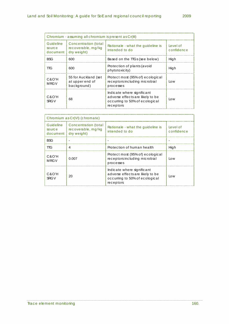
Land and Soil Monitoring: A guide for SoE and regional council reporting 2009
Trace element monitoring 160.
Chromium - assuming all chromium is present as Cr(III)
Guideline source document
Concentration (total recoverable, mg/kg dry weight)
Rationale - what the guideline is intended to do
Level of confidence
BSG 600 Based on the TTGs (see below) High
TTG 600 Protection of plants (avoid phytotoxicity) High
C&O'H MRGV
55 for Auckland (set at upper end of background)
Protect most (95% of) ecological receptors including microbial processes
Low
C&O'H SRGV 68
Indicate where significant adverse effects are likely to be occurring to 50% of ecological receptors
Low
Chromium as Cr(VI) (chromate)
Guideline source document
Concentration (total recoverable, mg/kg dry weight)
Rationale - what the guideline is intended to do
Level of confidence
BSG - - -
TTG 4 Protection of human health High
C&O'H MRGV 0.007
Protect most (95% of) ecological receptors including microbial processes
Low
C&O'H SRGV 20
Indicate where significant adverse effects are likely to be occurring to 50% of ecological receptors
Low

Land and Soil Monitoring: A guide for SoE and regional council reporting 2009
Trace element monitoring 161.
Copper
Guideline source document
Concentration (total recoverable, mg/kg dry weight)
Rationale - what the guideline is intended to do
Level of confidence
BSG 100
Protection of plants (avoid phytotoxicity). Authors indicate it should also protect soil microbial health and groundwater.
Medium
TTG 40, 130
40 mg/kg: protection of human health, but not regarded as reliable due to documented problems with guideline derivation. 130 mg/kg: protection of plants
Low for human health; High for plant protection
C&O'H MRGV
45 for Auckland (set at upper end of background)
Protect most (95% of) ecological receptors including microbial processes
Medium
C&O'H SRGV 135
Indicate where significant adverse effects are likely to be occurring to 50% of ecological receptors
High
Lead
Guideline source document
Concentration (total recoverable, mg/kg dry weight)
Rationale – what the guideline is intended to do
Level of confidence
BSG 300
Protect human health, plants, and grazing animals. Authors indicate it should also protect soil microbial health and groundwater.
Medium
TTG - - -
C&O’H MRGV
60 for Auckland (set at upper end of background)
Protect most (95% of) ecological receptors including microbial processes
High
C&O’H SRGV 100
Indicate where significant adverse effects are likely to be occurring to 50% of ecological receptors
High
CCME 70
Protect human and ecological health (agricultural soils). Currently selected as a contaminated land investigation threshold following CLMG#2 in the absence of New Zealand full risk-based guideline for human and ecological health.
High

Land and Soil Monitoring: A guide for SoE and regional council reporting 2009
Trace element monitoring 162.
Mercury
Guideline source document
Concentration (total recoverable, mg/kg dry weight)
Rationale - what the guideline is intended to do
Level of confidence
BSG 1
Set to remain in keeping with overseas limits for loading of biosolids. Should protect against uptake and bioaccumulation; considered to be conservative
Medium
TTG - - -
C&O'H MRGV 0.7
Protect most (95% of) ecological receptors including microbial processes
Low
C&O'H SRGV 65
Indicate where significant adverse effects are likely to be occurring to 50% of ecological receptors.
Medium
CCME 6.6
Protect human and ecological health (agricultural soils). Currently selected as a contaminated land investigation threshold following CLMG#2 in the absence of New Zealand full risk-based guideline for human and ecological health.
High
Nickel
Guideline source document
Concentration (total recoverable, mg/kg dry weight)
Rationale – what the guideline is intended to do
Level of confidence
BSG 60
Protection of plants (avoid phytotoxicity). Authors indicate it should also protect soil microbial health and groundwater.
Medium
TTG - - -
C&O’H MRGV
35 for Auckland (set at upper end of background)
Protect most (95% of) ecological receptors including microbial processes
Low
C&O’H SRGV 110
Indicate where significant adverse effects are likely to be occurring to 50% of ecological receptors.
Medium
CCME 50
Protect human and ecological health (agricultural soils). Currently selected as a contaminated land investigation threshold following CLMG#2 in the absence of New Zealand full risk-based guideline for human and ecological health.
High

Land and Soil Monitoring: A guide for SoE and regional council reporting 2009
Trace element monitoring 163.
Zinc
Guideline source document
Concentration (total recoverable, mg/kg dry weight)
Rationale - what the guideline is intended to do
Level of confidence
BSG 300 Protection of plants (avoid phytotoxicity). and soil microbial health.
Medium
TTG - - -
C&O'H MRGV
180 for Auckland (set at upper end of background)
Protect most (95% of) ecological receptors including microbial processes
Low
C&O'H SRGV 200
Indicate where significant adverse effects are likely to be occurring to 50% of ecological receptors.
High
CCME 200
Protect human and ecological health (agricultural soils). Currently selected as a contaminated land investigation threshold following CLMG#2 in the absence of New Zealand full risk-based guideline for human and ecological health.
High

Land and Soil Monitoring: A guide for SoE and regional council reporting 2009
Trace element monitoring 164.
Source document key Abbreviation Short title Full reference
TTG Timber Treatment Guidelines (1997)
Ministry for the Environment and Ministry of Health, 1997. Health and Environmental Guidelines for Selected Timber Treatment Chemicals
BSG Biosolids Guidelines (2003)
New Zealand Water and Wastes Association (NZWWA), 2003. Guidelines for the Safe Application of Biosolids to Land in New Zealand.
C&O'H MRGV
Cavanagh and O’Halloran Minimal Risk Guideline Value (2006)
Cavanagh JE and O’Halloran K, 2006. Development of Soil Guideline Values Protective of Ecological Receptors in the Auckland Region: Parts 1 and 2. Landcare Research Contract Reports: LC0506/065 and LC0506/179. Prepared for Auckland Regional Council.
C&O'H SRGV
Cavanagh and O’Halloran Serious Risk Guideline Value (2006)
Cavanagh JE and O’Halloran K, 2006. Development of Soil Guideline Values Protective of Ecological Receptors in the Auckland Region: Parts 1 and 2. Landcare Research Contract Reports: LC0506/065 and LC0506/179. Prepared for Auckland Regional Council.
CCME
Canadian Councils of Ministers of the Environment (2002)
CCME (Canadian Council of Ministers of the Environment), 2002. Canadian Environmental Quality Guidelines.
CLMG#2
Contaminated Land Management Guideline No.2
Ministry for the Environment, 2003. Contaminated Land Management Guideline No.2. Hierarchy and Application in New Zealand of Environmental Guideline Values.
Notes: 1. Guidelines are for agricultural land only. 2. For the essential elements, guidelines cover excess (rather than deficiency). 3. Overseas risk-based values are given only where a significant receptor class is
not covered by a New Zealand risk-based guideline. This follows the Ministry for the Environment's guideline hierarchy (CLMG#2) for assessing potentially contaminated land.
4. For the CCME guidelines, the adopted value is the lowest of either calculated value for human or ecological health, and therefore is protective of both.

Land and Soil Monitoring: A guide for SoE and regional council reporting 2009
Trace element monitoring 165.
6 References Auckland Regional Council, (2002). Background concentrations of inorganic
elements in soils from the Auckland Region. Auckland Regional Council Technical Publication No. 153. Auckland Regional Council, Auckland.
Environment Canterbury, (2007). Background concentrations of selected elements in Canterbury soils. Addendum 1:Additional samples and Timaru specific background levels. Environment Canterbury, 2007, Report R07/1/2.
Gaw, S.K., Kim, N.D., Northcott, G.L., Wilkins A.L., Robinson G. (2006). Developing site-specific guidelines for orchard soils based on bioaccessibility – can it be done? Waste Management Institute of New Zealand (WasteMINZ) Annual Conference, 8-9 November 2006, Christchurch.
Giltrap, D.J. and Hewitt, A.E. (2003). Spatial variability of soil quality indicators in New Zealand soils and land uses. New Zealand Journal of Agricultural Research 47, 167-177.
Holland, P. and Rahman, A. (1999). Review of trends in agricultural pesticide use in New Zealand. MAF Policy Technical Paper 99/11.
Kabata-Pendias, A. and Pendias, H. (2001). Trace elements in soils and plants, 3rd edition. CRC Press Boca Raton.
Kim, N.D. (2005). Cadmium accumulation in Waikato soils (Table 3). Environment Waikato technical report TR2005/51. Available from: http://www.ew.govt.nz/Publications/Technical-Reports/TR-200551/
Kim, N.D., Taylor, M.D., Chapman, R., Harris, J. and Robinson, P. (2008). Inadvertent sources of trace elements in Waikato’s rural soils. New Zealand Trace Elements Group Conference 2008. 13-15th February 2008, University of the Waikato, Hamilton, New Zealand. Available from: http://www.tracenz.net/conference2008/NZTEG2008_006.html
Marlborough District Council, (2007). Marlborough District Council Report. November 2007. Trace element concentrations in Marlborough soils.
Menzel, R.G. (1968). Uranium, radium and thorium content in phosphate rocks and their possible radiation hazard. J. Agr. Food Chem. 16, 231-234.
Mills, T., Robinson, B. and Clothier, B. (2004). The accumulation of heavy metals in Waikato’s productive sector environments. HortResearch Client Report 13155/2004. Final report to Environment Waikato. Hard copy: Environment Waikato Document 928390. Electronic Copy: Document 938788.
Ministry of Agriculture and Forestry, (2008). Report One: Cadmium in New Zealand Agriculture, report of the Cadmium Working Group. MAF Information Services, Wellington.
Ministry for the Environment, (2003). Contaminated Land Management Guidelines .1 Reporting on contaminated sites in New Zealand. Ministry for the Environment, Wellington.
Ministry for the Environment, (2004a). Contaminated Land Management Guidelines. 3 Risk screening system. Ministry for the Environment, Wellington.
Ministry for the Environment, (2004b). Contaminated Land Management Guidelines. 5 Site investigation and analysis of soils. Ministry for the Environment, Wellington.

Land and Soil Monitoring: A guide for SoE and regional council reporting 2009
Trace element monitoring 166.
Ministry for the Environment, (2006). Contaminated Land Management Guidelines. 4 Classification and information management protocols. Ministry for the Environment, Wellington.
Ministry for the Environment, (2007). Contaminated Land Management Guidelines. 2 Hierarchy and application of New Zealand of environmental guideline values. Ministry for the Environment, Wellington.
New Zealand Waste Water Association, (2003). Guidelines for the safe application of biosolids to land in New Zealand. Ministry for the Environment, Wellington, New Zealand.
Nriagu J.O. (1989). A global assessment of natural sources of atmospheric trace metals. Nature, 338, 47–49.
Percival, H.J., Webb, T.H. and Speir, T.W. (1996) Assessment of background concentrations of selected determinands in Canterbury soils. Landcare Research contract report: LC9596/133, Landcare Research, Lincoln.
Schipper, L.A. and Sparling, G.P. (2000). Performance of soil condition indicators across taxonomic groups and land uses. Soil Sci. Soc. Am. J. 64, 300-311.
Sparling, G., Schipper, L., Bettjeman, W. and Hill, R. (2004). Soil quality monitoring in New Zealand: practical lessons from a 6-year trial Agriculture, Ecosystems & Environment 104, 523-534.
Sulzberger, C. and Whitty. D. (2003). Determination of common pollutant background soil concentrations for the Wellington Region. URS, Wellington.