lagrangian-eulerian advection of noise and dye...

Lagrangian-Eulerian Advection of Noise andDye Textures for Unsteady Flow Visualization

Bruno Jobard, Gordon Erlebacher, and M. Yousuff Hussaini

Abstract—A new hybrid scheme (LEA) that combines the advantages of Eulerian and Lagrangian frameworks is applied to the

visualization of dense representations of time-dependent vector fields. The algorithm encodes the particles into a texture that is then

advected. By treating every particle equally, we can handle texture advection and dye advection within a single framework. High

temporal and spatial correlation is achieved through the blending of successive frames. A combination of particle and dye advection

enables the simultaneous visualization of streamlines, particle paths, and streaklines. We demonstrate various experimental

techniques on several physical flow fields. The simplicity of both the resulting data structures and the implementation suggest that LEA

could become a useful component of any scientific visualization toolkit concerned with the display of unsteady flows.

Index Terms—Flow visualization, texture advection, unsteady flow fields.

æ

1 INTRODUCTION

TRADITIONALLY, unsteady flow fields are thought of as acollection of pathlines or streaklines that originate from

user-defined seed points [9], [10]. These trajectories are oftenvisualized in experimental laboratories through the injectionof dye into the fluid [17]. Release of the dye can be continuousor pulsed, colored, locally concentrated, or spread out over anextended region. Proper use of dye makes it possible toextract quantitative information about the velocity magni-tude, direction, rate of strain tensor, and to visualizepathlines, streaklines, and timelines [7], [11], [13], [18].

At the other end of the spectrum, the use of denserepresentations of the flow as a means of maximizinginformation content has been attracting a lot of attention [3],[6], [7], [8], [12], [13], [15], [18]. In a time-dependent context,the fundamental challenge faced by this class of algorithmsis to produce smooth animations with good spatial andtemporal correlation.

In this paper, we describe a new algorithm based ondense representations of time-dependent vector fields andapply it to noise and dye advection. The method combinesthe advantages of the Lagrangian and Eulerian formalisms.Briefly stated, a dense set of particles is stored ascoordinates in a texture. Each iteration is defined by aLagrangian step (backward time integration of the particles)and a Eulerian step (update of the image pixel colors).Texture advection and dye advection are differentiatedchiefly by how the advected textures are defined. Allinformation is stored in a few two-dimensional arrays. Byits very nature, the algorithm takes advantage of spatial

locality and instruction pipelining and can generate anima-tions at interactive frame rates.

The rest of the paper is organized as follows: Section 2gives an overview of related work. The general approach isdescribed in Section 3, while the algorithm is examined inSections 4 (noise advection) and 5 (dye advection). Section 6discusses parameter selection. Timing results are presentedin Section 7. Conclusions are drawn in Section 8.

2 RELATED WORK

Several techniques have been advanced to produce denserepresentations of unsteady vector fields. Best known is,perhaps, UFLIC (Unsteady Flow LIC), developed by Shenand Kao [15] and based on the Line Integral Convolution(LIC) technique [2]. The algorithm achieves good spatialand temporal correlation. However, the images are difficultto interpret: The paths are blurred in regions of rapidchange of direction and are thickest where the flow isalmost uniform. The low performance of the algorithm isexplained by the large number of particles (three to fivetimes the number of pixels in the image) to process for eachanimation frame.

The spot noise technique, initially developed for thevisualization of steady vector fields, has a natural extensionto unsteady flows [3]. A sufficiently large collection ofelliptic spots is chosen to entirely cover an image of thephysical domain. The position of these spots is integratedalong the flow, bent along the local pathline or streamline,and finally blended into the animation frame. The render-ing speed of the algorithm can be increased by decreasingthe number of spots in the image. The control of pixelcoverage is done by assigning a fixed lifespan to each spot.

Max and Becker [12] propose a texture-based algorithmto represent steady and unsteady flow fields. The basic ideais to advect a texture along the flow either by advecting thevertices of a triangular mesh or by integrating the texturecoordinates associated with each triangle backward in time.When texture coordinates or particles leave the physical

IEEE TRANSACTIONS ON VISUALIZATION AND COMPUTER GRAPHICS, VOL. 8, NO. 3, JULY-SEPTEMBER 2002 211

. B. Jobard is with the Swiss Center for Scientific Computing, Via Cantonale,6928 Mano, Switzerland. E-mail: [email protected].

. G. Erlebacher and M.Y. Hussaini are with the School of ComputationalScience and Information Technology, Dirac Science Library, Florida StateUniversity, Tallahassee, FL 32306-4120.E-mail: {erlebach, myh}@csit.fsu.edu.

Manuscript received 15 Feb. 2002; revised 15 Mar. 2002; accepted 2 Apr.2002.For information on obtaining reprints of this article, please send e-mail to:[email protected], and reference IEEECS Log Number 116206.

1077-2626/02/$17.00 ß 2002 IEEE

domain, an external velocity field is linearly extrapolatedfrom the boundary. This technique attains interactive framerates by controlling the resolution of the underlying mesh.

A technique to display streaklines was developed byRumpf and Becker [13]. They precompute a two-dimen-sional noise texture whose coordinates represent time and aboundary Lagrangian coordinate. Particles at any point inspace and time that originate from an inflow boundary aremapped back to a point in this texture.

More recently, Jobard et al. [6], [7] extend the work ofHeidrich et al. [4] to animate unsteady two-dimensionalvector fields. The algorithm relies heavily on extensions toOpenGL proposed by SGI, in particular, pixel textures,additive and subtractive blending, and color transformationmatrices. They pay particular attention to the flow enteringand leaving the physical domain, leading to smoothanimations of arbitrary duration. Excessive discretizationerrors associated with 12 bit textures are addressed by atiling mechanism [6]. Unfortunately, the graphics hardwareextension this algorithm relies on most, the pixel textureextension, was not adopted by other graphics cardmanufacturers. As a result, the algorithm only runs on theSGI Maximum Impact and the SGI Octane with the MXEgraphics card. Application of LEA to flows with shocks isconsidered in Hussaini et al. [5]. Recently, a new algorithmbased on the Nvidia GeForce3 graphics card has beendeveloped for texture advection [18].

3 LAGRANGIAN-EULERIAN APPROACH

We wish to track a collection of particles, pi, along aprescribed time-dependent velocity field, that denselycovers a rectangular region. If we assign a property P ðpiÞto the ith particle pi, the property remains constant as theparticle follows its pathline. At any given instant t, eachspatial location x has an associated particle, labeled ptðxÞ.One expresses that the particle property is invariant along apathline by

@P ðptðxÞÞ@t

þ vtðxÞ � rP ðptÞðxÞÞ ¼ 0: ð1Þ

The property attached to each particle takes on the role ofa passive scalar. Its value is therefore not affected bydiffusion or source terms (associated with chemical or otherprocesses). This equation has two interpretations. In thefirst, the trajectory of a single particle, denoted by xtðpÞwhere p tags the particle, satisfies

dxtðpÞdt

¼ vtðxt; pÞ: ð2Þ

In this Lagrangian approach, the trajectory of eachparticle is computed separately. The time evolution of acollection of particles is displayed by rendering eachparticle by a glyph (point, texture spot [3], arrows). Exceptfor the recent work of Jobard et al. [5], [6], [7], [18], currenttime-dependent algorithms are all based on particle track-ing, e.g., [1], [3], [10], [12], [15]. While Lagrangian tracking iswell-suited to the task of understanding how dense groupsof particles evolve in time, it suffers from several short-comings. In regions of flow convergence, particles may

accumulate into small clusters that follow almost identicaltrajectories, leaving regions of flow divergence with a lowdensity of particles. To maintain dense coverage of thedomain, the data structures must support dynamic inser-tion and deletion of particles [15] or track more particlesthan needed [3], which decreases the efficiency of anyimplementation.

Alternatively, a Eulerian approach solves (1) directly.Particles lose their identity. However, the particle property,viewed as a field, is known for all time at any spatialcoordinate. Unfortunately, any explicit discretization of (1)is subject to a Courant condition1 so that, in practice, thenumerical integration step is limited to at most one to twocell widths. In turn, this imposes a maximum rate at whichflow structures can evolve.

In our approach, we choose a hybrid solution. Betweentwo successive time steps, coordinates of a dense collectionof particles are updated with a Lagrangian scheme, whereasthe advection of the particle property is achieved with aEulerian method. At the beginning of each iteration, a newdense collection of particles is chosen and assigned theproperty computed at the end of the previous iteration. Werefer to the hybrid nature of this approach as a Lagrangian-Eulerian Advection (LEA) method.

To illustrate the idea, consider the advection of thebitmap image shown in Fig. 1a by a circular vector fieldcentered at the lower left corner of the image. With a pureLagrangian scheme, a dense collection of particles (one perpixel) is first assigned the color of the correspondingunderlying pixel. Each particle advects along the vectorfield and deposits its color property in the correspondingpixel in a new bitmap image. This technique does notensure that every pixel of the new image is updated.Indeed, holes usually appear in the resulting image (Fig. 1b).

A better scheme considers each pixel of the new image asa particle whose position is integrated backward in time.The particle position in the initial bitmap determines itscolor. There are no longer any holes in the new image(Fig. 1c). Repeating the process at each iteration, anyproperty can be advected while maintaining a densecoverage of the domain.

The core of the advection process is thus the compositionof two basic operations: coordinate integration and propertyadvection.

212 IEEE TRANSACTIONS ON VISUALIZATION AND COMPUTER GRAPHICS, VOL. 8, NO. 3, JULY-SEPTEMBER 2002

1. If the discrete time step exceeds some maximum value, severenumerical instabilities result.

Fig. 1. Rotation of bitmap image about the lower left corner. (a) Original

image. (b) Image rotated with Lagrangian scheme. (c) Image rotated

with Eulerian scheme.

Given the position x0ði; jÞ ¼ ði; jÞ of each particle in thenew image, backward integration of (2) over a time intervalh determines its position

xÿh i; jð Þ ¼ x0 i; jð Þ þZÿh0

vtÿ� x� i; jð Þð Þd� ð3Þ

at a previous time step. h is the integration step, x� ði; jÞrepresents intermediary positions along the pathlinepassing through xtði; jÞ and v� is the vector field at time � .

An image of resolution W �H, defined at a previoustime tÿ h, is advected to time t through the indirectionoperation

Itði; jÞ ¼ Itÿhðxÿhði; jÞÞ 8xÿh 2 ½0;WÞ � ½0; HÞuser-specified value otherwise;

�ð4Þ

which allows the image at time t to be computed from theimage at any prior time tÿ h. This technique was used byMax and Becker [12]. However, instead of integrating backto the initial time to advect the same initial texture [12], wechoose h to be the interval between two successivedisplayed images and always advect the last computedimage. This minimizes the need to access coordinate valuesoutside the physical domain. Notice that at least a linearinterpolation of Itÿh pixels at the positions xÿh is necessaryto obtain an image of acceptable quality.

In the next two sections, we describe noise-based anddye-based advection methods.

4 NOISE-BASED ADVECTION

With our Lagrangian-Eulerian approach, a full per-pixeladvection requires manipulating exactly W �H particles.All information concerning any particle is stored in two-dimensional arrays with resolution W �H at the corre-sponding location i; jð Þ. Thus, we store the initial coordi-nates x; yð Þ of those particles in two arrays Cx i; jð Þ andCy i; jð Þ. Two arrays C0x and C0y contain their x andy coordinates after integration. A first order integrationmethod requires two arrays Vx and Vy that store thevelocity field at the current time. Similarly to LIC, wechoose to advect noise images. Four noise arrays N, N0, Na,and Nb contain, respectively, the noise to advect, twoadvected noise images, and the final blended image.

Fig. 2 shows a flowchart of the algorithm. After theinitialization of the coordinate and noise arrays (Section 4.2),the coordinates are integrated (Section 4.3) and the initialnoise array N is advected (Section 4.4). The first advectednoise array, N0 is then prepared for the next iteration bysubjecting it to a series of treatments (left column in Fig. 2).Care is first taken to ensure that no spurious artifactsappear at boundaries where flow enters the domain(Section 4.5). This is followed by an optional maskingprocess to allow for nonrectangular domains (Section 4.6).A low percentage of random noise is then injected into theflow to compensate for the effects of pixel duplication andflow divergence (Section 4.7). Finally, the coordinate arraysare reinitialized to ready them for the next iteration(Section 4.8). The right column in the flowchart describesthe sequence of steps that transform the second advected

noise array Na into the final image. Na is first accumulated

into Nb via a blending operation to create the necessary

spatio-temporal correlation (Section 4.9). Three optional

postprocessing phases are then applied to Nb before its final

display: A line integral convolution filter removes aliasing

effects (Section 4.10.1) and features of interest are empha-

sized via an opacity mask (Section 4.10.2).

4.1 Notation

Array cell values are referenced by the notation A i; jð Þwith i

and j integers in 0; ::;W ÿ 1f g � 0; ::; H ÿ 1f g. We adopt the

convention that an array A x; yð Þ with real arguments is

evaluated from information in the four neighboring cells

using bilinear interpolation. A constant interpolation is

explicitly noted A xb c; yb cð Þ, where xb c is the largest integer

smaller than or equal to x. To simplify the notation, array

operations such as A ¼ B apply to the entire domain of ði; jÞ.The indirection operation A i; jð Þ ¼ B rC i; jð Þ; sD i; jð Þð Þ,

where Cði; jÞ and Dði; jÞ lie in the range 0;W ÿ 1½ � and

0; H ÿ 1½ �, respectively, and r and s are scalars, is denoted

by A ¼ B rC; sDð Þ.

4.2 Coordinate and Noise Initialization

We first initialize the coordinate arrays Cx, Cy and the noise

arrays N and Nb. Coordinates are initialized by

Csði; jÞ ¼ iþ randð1ÞCyði; jÞ ¼ jþ randð1Þ;

�ð5Þ

where randð1Þ is a real number in 0; 1½ Þ. The random offset

distributes coordinates on a jitter grid to avoid regular

patterns that might otherwise appear during the first

several steps of the advection. Note that the integer part

of each coordinate serves as an index into the cell.N is initialized with a two-valued noise function (0 or 1) to

ensure maximum contrast and its values are copied into Nb.

Coordinates and noise values are stored in floating-point

format to ensure sufficient accuracy in the calculations.

JOBARD ET AL.: LAGRANGIAN-EULERIAN ADVECTION OF NOISE AND DYE TEXTURES FOR UNSTEADY FLOW VISUALIZATION 213

Fig. 2. Flowchart of LEA algorithm.

4.3 Coordinate Integration

A first order discretization of (3) with a constant time step hgives

C0x ¼ Cx ÿ ðlmax=VmaxÞVxðrWVCx; rHV

CyÞC0y ¼ Cy ÿ ðlmax=VmaxÞVyðrHW

Cx; rHVCyÞ;

�ð6Þ

where rWV¼ WV ÿ 1ð Þ=W and rHV

¼ HV ÿ 1ð Þ=H for avector field resolution of WV by WH . The two scalingfactors rWV

and rHVensure that the coordinates of the

velocity arrays stay within proper bounds. We replaced theconstant integration time step h with the quotient lmax=Vmax,where Vmax is the maximum velocity magnitude over theentire space-time domain. Therefore, the new quantity lmax

represents the maximal possible displacement of a particleover all iterations, measured in units of cell widths. Theactual displacement of a particle is proportional to the localvelocity, also measured in cell widths. The velocity arraysVx and Vy at the current time are linearly interpolatedbetween the two closest available vector fields in the dataset. Section 6 discusses the relationship between parametersnecessary to generate animations consistent with thephysics of the problem.

A useful property of a first order formulation is that thevelocity arrays are never accessed at a point outside thephysical domain. We have also implemented a second orderdiscretization, but found no noticeable improvement due tothe small extent of the spatio-temporal correlations in thefinal display. However, high accuracy is important for dyeadvection (Section 5).

4.4 Noise Advection

The advection of noise described by (4) is applied twice toN to produce two noise arrays N0 and Na, one foradvection, one for display. N0 is an internal noise arraywhose purpose is to carry on the advection process and toreinitialize N for the next iteration. To maintain asufficiently high contrast in the advected noise, N0 iscomputed with a constant interpolation. Before N0 can beused in the next iteration, it must undergo a series ofcorrections to account for edge effects, the presence ofarbitrary domains, and the deleterious consequences offlow divergence.

Na serves to create the current animation frame and nolonger participates in the noise advection. It is computedusing linear interpolation of N to reduce spatial aliasingeffects. Na is then blended into Nb (Section 4.9).

A straightforward implementation of (4) leads to condi-tional expressions to handle the cases when

x0 i; jð Þ ¼ C0x i; jð Þ;C0y i; jð Þÿ �

is exterior to the physical domain. A more efficientimplementation eliminates the need to test for boundaryconditions by surrounding N and N0 with a buffer zone ofconstant width. From (6), x0 i; jð Þ refers to cells located atmost a distance of b ¼ hd e cell widths away from the arrayborders. An expanded noise array of size W þ 2bð Þ �H þ 2bð Þ is therefore sufficient to prevent out of bound

array accesses (see Fig. 3). The advected arrays N0 and Na

are computed according to

N0ðiþ b; jþ bÞ ¼ N C0xði; jÞ� �

þ b; C0yði; jÞj k

þ b� �

Naði; jÞ ¼ N rWC0xði; jÞ þ b; rHC0yði; jÞ þ b� �

;

8<: ð7Þ

for all i; jð Þ 2 0; ::;W ÿ 1f g � 0; ::; H ÿ 1f g, where rW ¼W ÿ 1ð Þ=W and rH ¼ H ÿ 1ð Þ=H. The two scaling factorsrW and rH ensure a properly constructed linear interpolation.

4.5 Edge Treatment

A recurring issue with texture advection that must beaddressed is the proper treatment of information flowinginto the physical domain. Within the context of this paper,we must determine the user-specified value in (4). Toaddress this, we recall that the advected image contains atwo-valued random noise with little or no spatial correla-tion. We take advantage of this property to replace the user-specified value by a random value (0 or 1). At each iteration,we simply store new random noise in the buffer zone, atnegligible cost.

At the next iteration, N will contain these values andsome of them will be advected to the interior of the physicaldomain by (7). Since random noise has no spatial correla-tion, the advection of the surrounding buffer values into theinterior region of N0 produces no visible artifacts.

To treat periodic flows in one or more directions, thenoise values are copied from an inner strip of width b alongthe interior edge of N0 onto the buffer zone at the oppositeboundary. As a result, particles leaving one side of thedomain seamlessly reappear at its opposite side.

4.6 Incoming Flow in Arbitrary Shaped Domains

It often happens that the physical domain is nonrectangularor contains interior regions where the flow is not defined.Denote by B the boundaries interior to N that delineatesthese regions. LEA handles this case with no modificationby simply setting the velocity to zero where it is notdefined. The stationary noise in these regions is hiddenfrom the animation frame by superimposing a semitran-sparent map that is opaque where the flow is undefined.For example, the opaque regions of this map mightrepresent shorelines or islands.

When the flow velocity normal to B is nonzero andpoints into the physical domain, the advection of stationarynoise values will create noticeable artifacts in the form ofstreaks. This might happen if an underground flow, notvisible in the display, emerges into view at B. If necessary,we suppress these streaks with the help of a precomputedBoolean mask (or, alternatively, a Boolean function) M i; jð Þthat determines whether or not the velocity field is defined


Fig. 3. Noise arrays N0 and Na are expanded with a surrounding region

b ¼ hd e cells wide.

at ði; jÞ. N0 i; jð Þ is then updated with random noise whereM i; jð Þ is false.

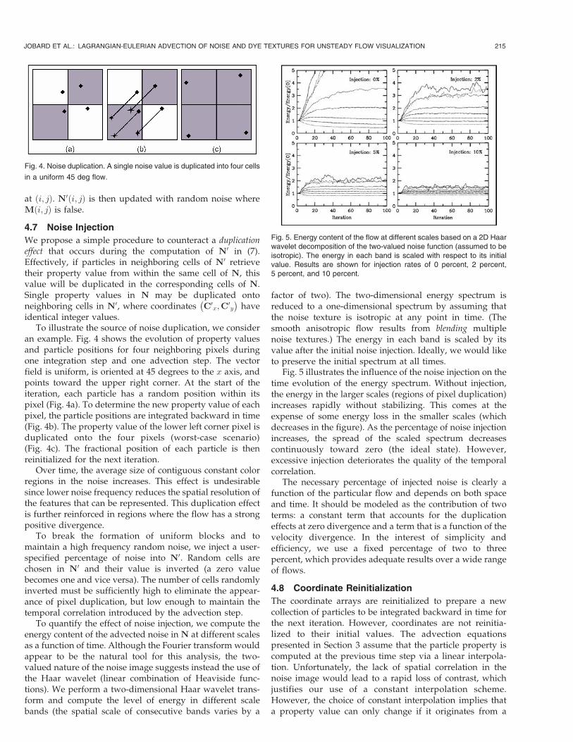
4.7 Noise Injection

We propose a simple procedure to counteract a duplicationeffect that occurs during the computation of N0 in (7).Effectively, if particles in neighboring cells of N0 retrievetheir property value from within the same cell of N, thisvalue will be duplicated in the corresponding cells of N.Single property values in N may be duplicated ontoneighboring cells in N0, where coordinates C0x;C

0y

ÿ �have

identical integer values.To illustrate the source of noise duplication, we consider

an example. Fig. 4 shows the evolution of property valuesand particle positions for four neighboring pixels duringone integration step and one advection step. The vectorfield is uniform, is oriented at 45 degrees to the x axis, andpoints toward the upper right corner. At the start of theiteration, each particle has a random position within itspixel (Fig. 4a). To determine the new property value of eachpixel, the particle positions are integrated backward in time(Fig. 4b). The property value of the lower left corner pixel isduplicated onto the four pixels (worst-case scenario)(Fig. 4c). The fractional position of each particle is thenreinitialized for the next iteration.

Over time, the average size of contiguous constant colorregions in the noise increases. This effect is undesirablesince lower noise frequency reduces the spatial resolution ofthe features that can be represented. This duplication effectis further reinforced in regions where the flow has a strongpositive divergence.

To break the formation of uniform blocks and tomaintain a high frequency random noise, we inject a user-specified percentage of noise into N0. Random cells arechosen in N0 and their value is inverted (a zero valuebecomes one and vice versa). The number of cells randomlyinverted must be sufficiently high to eliminate the appear-ance of pixel duplication, but low enough to maintain thetemporal correlation introduced by the advection step.

To quantify the effect of noise injection, we compute theenergy content of the advected noise in N at different scalesas a function of time. Although the Fourier transform wouldappear to be the natural tool for this analysis, the two-valued nature of the noise image suggests instead the use ofthe Haar wavelet (linear combination of Heaviside func-tions). We perform a two-dimensional Haar wavelet trans-form and compute the level of energy in different scalebands (the spatial scale of consecutive bands varies by a

factor of two). The two-dimensional energy spectrum isreduced to a one-dimensional spectrum by assuming thatthe noise texture is isotropic at any point in time. (Thesmooth anisotropic flow results from blending multiplenoise textures.) The energy in each band is scaled by itsvalue after the initial noise injection. Ideally, we would liketo preserve the initial spectrum at all times.

Fig. 5 illustrates the influence of the noise injection on thetime evolution of the energy spectrum. Without injection,the energy in the larger scales (regions of pixel duplication)increases rapidly without stabilizing. This comes at theexpense of some energy loss in the smaller scales (whichdecreases in the figure). As the percentage of noise injectionincreases, the spread of the scaled spectrum decreasescontinuously toward zero (the ideal state). However,excessive injection deteriorates the quality of the temporalcorrelation.

The necessary percentage of injected noise is clearly afunction of the particular flow and depends on both spaceand time. It should be modeled as the contribution of twoterms: a constant term that accounts for the duplicationeffects at zero divergence and a term that is a function of thevelocity divergence. In the interest of simplicity andefficiency, we use a fixed percentage of two to threepercent, which provides adequate results over a wide rangeof flows.

4.8 Coordinate Reinitialization

The coordinate arrays are reinitialized to prepare a newcollection of particles to be integrated backward in time forthe next iteration. However, coordinates are not reinitia-lized to their initial values. The advection equationspresented in Section 3 assume that the particle property iscomputed at the previous time step via a linear interpola-tion. Unfortunately, the lack of spatial correlation in thenoise image would lead to a rapid loss of contrast, whichjustifies our use of a constant interpolation scheme.However, the choice of constant interpolation implies thata property value can only change if it originates from a


Fig. 4. Noise duplication. A single noise value is duplicated into four cells

in a uniform 45 deg flow.

Fig. 5. Energy content of the flow at different scales based on a 2D Haarwavelet decomposition of the two-valued noise function (assumed to beisotropic). The energy in each band is scaled with respect to its initialvalue. Results are shown for injection rates of 0 percent, 2 percent,5 percent, and 10 percent.

different cell. If the coordinate arrays were reinitialized totheir original values at each iteration, subcell displacementswould be ignored and the flow would be frozen where thevelocity magnitude is too low. This is illustrated in Fig. 6,which shows the advection of a steady circular vector field.Constant interpolation without fractional coordinate track-ing clearly shows that the flow is partitioned into distinctregions within which the integer displacement vector isconstant (Fig. 6a).

To prevent this from happening, we track thefractional part of the displacement within each cell.Instead of reinitializing the coordinates to their initialvalues, the fractional part of the displacement isadded to cell indices ði; jÞ:

Cxði; jÞ ¼ iþC0xði; jÞ ÿ bC0xði; jÞcCyði; jÞ ¼ jþC0yði; jÞ ÿ bC0yði; jÞc:

�ð8Þ

The effect of this correction is shown in Fig. 6b.The coordinate arrays have now returned to the state

they were in after their initialization phase ((5); they verifythe relations Cx i; jð Þb c ¼ i and Cy i; jð Þ

� �¼ j.

4.9 Noise Blending

Although successive advected noise arrays are correlated intime, each individual frame remains devoid of spatialcorrelation. By applying a temporal filter to successiveframes, spatial correlation is introduced. We store the resultof the filtering process in an array Nb. We have found theexponential filter to be convenient since its discrete versiononly requires the current advected noise and the previousfiltered frame. It is implemented as an alpha blendingoperation

Nb ¼ ð1ÿ �ÞNb þ �Na; ð9Þ

where � represents the opacity of the current advectednoise array. A typical range for � is 0:05; 0:2½ �. Fig. 7 showsthe effect of � on images based on the same set of noisearrays.

The blending stage is crucial because it introduces spatialcorrelation along pathline segments in every frame. To showclearly that the spatial correlation occurs along pathlinespassing through each cell, we conceptualize the algorithmin 3D space; the x and y axes represent the spatialcoordinates, whereas the third axis is time. To understand

the effect of the blending operation, let’s consider an array Nwith black cells and change a single cell to white. Duringadvection, a sequence of noise arrays (stacked along thetime axis) is generated in which the white cell is displacedalong the flow. By construction, the curve followed by thewhite cell is a pathline. The temporal filter blendssuccessive noise arrays Na with the most recent dataweighted more strongly. The temporal blend of these noisearrays produces the projection of the pathline onto the xÿ yplane, with an exponentially decreasing intensity as onetravels back in time along the pathline. When the noisearray with a single white cell is replaced by a two-colornoise distribution, the blending operation introduces spatialcorrelation along a dense set of short pathlines.

Streamlines and pathlines passing through the same cellat the same time are tangent to each other, so a streamline ofshort extent is well-approximated by a short pathline.Therefore, the collection of short pathlines serves toapproximate the instantaneous direction of the flow. Withour LEA technique, a single frame represents the instanta-neous structure of the flow (streamlines), whereas ananimated sequence of frames reveals the motion of a densecollection of particles released into the flow.

The filtering phase completes one pass of the advectionalgorithm. The image Nb can be displayed to the screen orstored as an animation frame. N0 is used as the initial noisetexture N for the next iteration. It is worthwhile to mentionthat each iteration ends with data having the exact sameproperty as when it started. In particular, the coordinatearrays satisfy

bCxði; jÞc ¼ i; bCyði; jÞc ¼ j

and N contains a two-color noise without degradation ofcontrast.

4.10 Postprocessing

A series of optional postprocessing steps is applied to Nb toenhance the image quality and to remove features of theflow that are uninteresting to the user. We present two


Fig. 6. Circular flow without and with accumulation of fractional

displacement (h = 2).

Fig. 7. Frames obtained with different values of �.

filters. A fast version of LIC can be applied to remove high

frequency content in the image, while a velocity mask serves

to draw attention to regions of the flow with strong

currents.

4.10.1 Directional Low-Pass Filtering (LIC)

Although the temporal filter (noise blending phase)

converts high frequency noise images into smooth spatially

correlated images, aliasing artifacts remain visible in

regions where the noise is advected over several cells in a

single iteration. As a rule, aliasing artifacts become notice-

able where noise advect more than one or two cells in a

single time step (see Fig. 8, bottom). Experimentation with

different low-pass filters led us to conclude that a Line

Integral Convolution filter applied to Nb is the best filter to

remove the effect of artifacts while preserving and enhan-

cing the directional correlation resulting from the blending

phase. This follows from the fact that temporal blending

and LIC bring out the structure of pathlines and stream-

lines, respectively, and these curves are tangent to one

another at each point. Although the image quality is often

enhanced with longer kernel lengths, it is detrimental here

since the resulting streamlines will have significant devia-

tions from the actual pathlines. The partial destruction of

the temporal correlation between frames would then lead to

flashing effects in the animation. A secondary effect of

longer kernels is decreased contrast.While any LIC implementation can be used, our

algorithm can advect an entire texture at interactive rates.

Therefore, we are interested in the fastest possible LIC

implementation. To the best of our knowledge, FastLIC [16]

and Hardware-Accelerated LIC [4] are the fastest algo-

rithms to date and both are well-suited to the task.

However, we propose a simple, but very efficient, software

version of Heidrich’s hardware implementation to post-

process the data when the highest quality is desired.Besides the input noise array Nb, the algorithm requires

two additional coordinate arrays, Cxx and Cyy, and an array

NLIC to store the result of the line integral convolution. The

length of the convolution kernel is denoted by L. For

reference, we include the pseudocode for Array-LIC in Fig. 9.In general, L � h produces a smooth image with no

aliasing. However, large values of h speed up the flow, with

a resulting increase in aliasing effects. If the quality of the

animation is important, L must be increased, with a

resulting slowdown in the frame rate. The execution time

of the LIC filter is commensurate with the timings of

FastLIC for L < 10. Beyond 10, a serial FastLIC [16] should

be used instead. An OpenMP implementation of our ALIC

algorithm on shared memory architectures is straightfor-

ward. Results are presented in Section 7. As shown in

Table 1, smoothing the velocity field with LIC reduces the

frame rate by a factor of three across architectures. We

recommend exploring the data at higher resolution without

the filter or at low resolution with the filter.

4.10.2 Velocity Mask

A straightforward implementation of the texture advection

algorithm described so far produces static images that show

the flow streamlines and interactive animations that show

the motion for the flow along pathlines. The length of the

streaks is statistically proportional to the flow velocity

magnitude. Additional information can be encoded into the

images by modulating the color intensity according to one

or more secondary variables.It is often advantageous to superimpose the representa-

tion of flow advection over a background image that

provides additional context. Two examples are shown in

Fig. 10. In order to implement this capability, the image

must become partially transparent.Two approaches have been implemented. First, we

couple the opacity of a pixel to its color intensity. Second,

we modulate the pixel transparency with the magnitude of

the velocity.


Fig. 8. Frame without (bottom) and with (top) LIC filter. A velocity mask if

applied to both images.

Fig. 9. Pseudocode for ALIC (Array LIC).

The blended image pixel color ranges from black towhite. Neither color has a predominant role in representingthe velocity streaks. Therefore, one of these colors can beeliminated and made partially transparent. We consider ablack pixel to be transparent and a white pixel to be fullyopaque. The transfer function that links these two states is apower law. Regions of the flow that are nearly stationaryadd little useful information to the view. For example,regions of high velocity are often of most interest in windand ocean current data. Accordingly, we also modulate thetransparency of each pixel according to the velocitymagnitude. This produces a strong correlation betweenthe length of the velocity streaks and their opacity.

The ideas described in the two previous paragraphs areimplemented through an opacity map, also referred to as avelocity mask. Once computed, the velocity mask is com-bined with Nb into an intensity-alpha texture that is blendedwith the background image. We define the opacity map

A ¼ 1ÿ 1ÿVð Þmð Þ 1ÿ 1ÿNbð Þnð Þ ð10Þ

as a product of a function of local velocity magnitude and afunction of the noise intensity. Higher values of theexponents m and n increase the contrast between regionsof low and high velocity magnitude and low and highintensity, respectively. When m ¼ n ¼ 1, the opacity mapreduces to

A ¼ VNb:

As the exponents are increased, the regions of highvelocity magnitude and of high noise intensity increasetheir importance relative to other regions in the flow.

Higher quality pictures that emphasize the velocitymagnitude can also be obtained by replacing the noisetexture with a scalar map of the velocity magnitude (withcolor ranging from black to white as the magnitude rangesfrom zero to one) with an opacity defined by (8). As a result,the texture advection is seen through the opacity map.

5 DYE-BASED ADVECTION

By replacing the advected noise texture by a texture with a

smooth pattern, one can emulate the process of dye

advection, a standard technique used in experimental flow

dynamics [17]. In this approach, a dye is released into the

flow and advected with the fluid. Dye advection has been

considered outside the context of texture advection techni-

ques [11], [14]. Standard approaches include tracking

clouds of particles or defining the dye with a polygonal

enclosure. More recently, dye has been incorporated within

the framework of texture advection schemes simply by

including the dye into the advected texture [7], [18]. If the

noise texture is replaced by a texture of uniform back-

ground color upon which the dye is deposed, the high

frequency nature of the texture is removed. As a result,

many of the treatments detailed in Section 4 are no longer

required and the implementation is greatly simplified. The

principal assumption in dye advection is that the color of

the texture varies smoothly in space.Effects that can safely be neglected include particle

injection into the edge buffer, random particle injection,


TABLE 1Timings in Frames/Second as a Function

of Options and Resolutions

Each configuration has been tested on four different configurations: PCworkstation (Xeon Dell Precision Workstation 530, 1.7 GHz, 1GB,256KM L2 cache) (upper left), Octane (SGI Octane, R12000, 300MHZ,2GB, 2MB L2 cache, 64KB L1 cache) (upper right), Onyx2 (SGI Onyx2,R12000, 300MHz, 2GB, 8MB L2 cache, 64KB L1 cache) (lower left), andOnyx2 with four processors (lower right).

Fig. 10. Noise-based advection with velocity mask and LIC filtering. Top:

Sea currents in the Gulf of Mexico (data courtesy of COAPS, Florida

State University). Bottom: Cyclone formation over Europe (data courtesy

of MeteoSwiss, Switzerland).

constant interpolation of the noise texture, coordinatereinitialization, and noise blending. We introduce here twonew arrays D and D0 that contain the dye at times t and tþ h.

5.1 Dye Injection

Starting from a background texture of uniform color, weinject, at every iteration, dye into the fluid. The injection isoften localized in space and assumes the shape of spots orcurves distributed across the fluid. The dye can be releasedonce and tracked (which approximates the path of aparticle), released continuously at a single point (generatesa streakline), or pulsated (the dye is turned on intermit-tently). To better discern the resulting patterns, colored dyeis very useful. In this case, three-color components must beindependently advected.

5.2 Dye Advection

The algorithm is similar to that used to advect the noisetexture. However, when advecting dye, it is important toaccurately track its long-time evolution. High order timeintegration schemes are therefore desirable. We havefound that a second order Runge-Kutta midpoint algo-rithm provides sufficient accuracy. The scheme introducesan intermediate time step and an associated intermediateposition x�. Although always within the extendedphysical, the velocity field at x� might not be defined.To avoid this situation, we set x0 ¼ x� whenever x� isoutside the physical domain.

A second order algorithm offers no particular advan-tages for noise-based texture advection schemes since theaccumulated error over the length of a typical streak isimperceptible. Noise-based representations cannot giveclear information about the origin of a particle and itsdestination. When dye is released into the flow at a point, itssubsequent trajectory lies along a particle path and theaccumulation of error due to an inaccurate time integrationscheme is very noticeable. Fig. 11 compares the result offirst and second order integration schemes on the trajectoryof dye continuously released into a circular flow. Unlike thefirst order scheme, the second order scheme producesclosed circles.

In noise advection schemes, constant interpolation of thecoordinate position was necessary to maintain maximumcontrast in the advected texture, which led to the notion ofsubcell particle tracking (Section 4.8). Because of thesmoothness of the dye images, we can directly apply the

advection scheme defined by (4). New property values ofD0 are linearly interpolated at position x0 in D. With linearinterpolation, subcell coordinates are no longer required; ateach iteration, the integration proceeds from the lower leftcorner of each cell. Coordinate arrays are not necessary fordye advection.

The new property of D0 cells is then computed from Daccording to

D0 iþ b; jþ bð Þ ¼ D rWx0xði; jÞ þ b; rHx0yði; jÞ þ bÿ �

for all i; jð Þ 2 0; ::;W ÿ 1f g � 0; ::; H ÿ 1f g. rH and rW coeffi-cients are defined in Section 4.4. x0kði; jÞ is the k component ofthe backward integration from coordinates i; jð Þ.

The dye advection proceeds independently from thenoise advection and the two resulting textures Nb and D0

can be combined to form composite images.During the advection phase, new property values in D0

are linearly interpolated from D. Since the dye color nowincludes contributions from neighboring pixels with thebackground color, the dye is numerically diffused, produ-cing a smoke-like effect. Although sometimes useful, thereare times when we wish the dye to retain its sharp interfacewith the background flow. One solution to counter thisproblem is presented in the next section.

5.3 Diffusion Correction

The operation of linear interpolation acts as a smooth filter.A cross section of a white spot over a black backgroundwould show an intensity profile that gets progressivelysmoother as the dot is advected. To maintain a sharpprofile, each color component could be corrected accordingto the simple prescription

if c < 0:5 then c ¼ 0 else c ¼ 1

for each color component c 2 0; 1½ �. However, this simplefunction produces excessive aliasing effects. Instead, wedesigned a filter function to steepen the smoothed profiletoward the ideal discontinuous profile that would result inthe absence of diffusion errors. Imposed constraints are thatc ¼ 0; 0:5; 1 be invariant to the filter. The rational function

c0 ¼ cÿ 1=2

sð2jcÿ 1=2j ÿ 1Þ þ 1þ 1=2;

with the sharpness parameter s 2 0; 1½ �, satisfies all therequirements. The identity function is recovered whens ¼ 0, while the simple thresholding function correspondsto s ¼ 1.

Fig. 12 shows the effect of diffusion on the advectionof a 16 pixel-wide square spot of dye along a circularvector field rotating clockwise and centered at x ¼ 0. Eachtime step (h ¼ 25), the dye is released at four evenlyspaced points along x ¼ 0. The sharpness parameter iss ¼ 0; 0:2; 0:5; 1. The sharpness is clearly improved whenthe filter is turned on. However, undesirable artifacts areclearly visible when s ¼ 1. We have found that s ¼ 0:2 is theminimum acceptable value.

A downside to the correction filter is that some dye isremoved that is not within the diffused region. The effect ismore noticeable if there are an insufficient number of pixelsin the regions with dye. In Fig. 13, dye is released into the


Fig. 11. Dye advection in a circular flow. (a) First order time integration.

(b) Second order time integration.

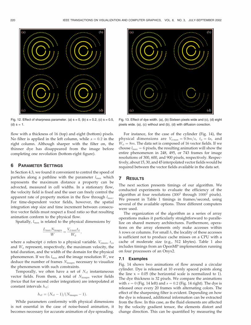
flow with a thickness of 16 (top) and eight (bottom) pixels.

No filter is applied in the left column, while s ¼ 0:2 in the

right column. Although sharper with the filter on, the

thinner dye has disappeared from the image before

completing one revolution (bottom-right figure).

6 PARAMETER SETTINGS

In Section 4.3, we found it convenient to control the speed of

particles along a pathline with the parameter lmax which

represents the maximum distance a property can be

advected, measured in cell widths. In a stationary flow,

the velocity field is fixed and the user can freely control the

apparent rate of property motion in the flow through lmax.

For time-dependent vector fields, however, the spatial

integration step size and time increment between consecu-

tive vector fields must respect a fixed ratio so that resulting

animation conform to the physical flow.Spatially, lmax is related to the physical dimensions by

LmaxNimages

W¼ V�maxt�

W�;

where a subscript � refers to a physical variable. V�max, t�,

and W� represent, respectively, the maximum velocity, the

total duration, and the width of the domain for the physical

phenomenon. If we fix lmax and the image resolution W , we

deduce the number of frames Nimages necessary to visualize

the phenomenon with such constraints.Temporally, we often have a set of Nvf instantaneous

vector fields. From them, a total of Nimages vector fields

(twice that for second order integration) are interpolated at

constant intervals hvf :

hvf ¼ ðNvf ÿ 1Þ=ðNimages ÿ 1Þ:

While parameters conformity with physical dimensions

is not essential in the case of noise-based animation, it

becomes necessary for accurate animation of dye spreading.

For instance, for the case of the cylinder (Fig. 14), thephysical dimensions are V�max ¼ 9:9m=s, t� ¼ 4s, andW� ¼ 8m. The data set is composed of 16 vector fields. If wechoose lmax ¼ 6 pixels, the resulting animation will show theentire phenomenon in 248, 495, or 743 frames for imageresolutions of 300, 600, and 900 pixels, respectively. Respec-tively, about 15, 30, and 45 interpolated vector fields would berequired between the vector fields available in the data set.

7 RESULTS

The next section presents timings of our algorithm. Weconducted experiments to evaluate the efficiency of thealgorithm at four resolutions (3002 through 10002 pixels).We present in Table 1 timings in frames/second, usingseveral of the available options. Three different computerswere used.

The organization of the algorithm as a series of arrayoperations makes it particularly straightforward to paralle-lize on shared memory architectures. Furthermore, opera-tions on the array elements only make accesses withinh rows or columns. For small h, the locality of these accessesis sufficient not to produce cache misses on a CPU with acache of moderate size (e.g., 512 kbytes). Table 1 alsoincludes timings from an OpenMP implementation runningon four processors of an Onyx2.

7.1 Examples

Fig. 14 shows two animations of flow around a circularcylinder. Dye is released at 10 evenly spaced points alongthe line x = 0.05 (the horizontal scale is normalized to 1).The dye thickness is 32 pixels. We compare the animationswith s ¼ 0 (Fig. 14 left) and s ¼ 0:2 (Fig. 14 right). The dye isreleased once every 20 frames with alternating colors. Theeffect of the sharpening filter is evident. Depending on howthe dye is released, additional information can be extractedfrom the flow. In this case, as the fluid elements are affectedby the velocity gradient tensor, the elements distort andchange direction. This can be quantified by measuring the


Fig. 12. Effect of sharpness parameter. (a) s = 0, (b) s = 0.2, (c) s = 0.5,

(d) s = 1.

Fig. 13. Effect of dye width. (a), (b) Sixteen pixels wide and (c), (d) eight

pixels wide. (a), (c) without and (b), (d) with diffusion corection.

change in area and shape in a postprocessing step. Only dye

advection is capable of providing this type of data. Note

that continuous dye release alone cannot provide this

information.Another example of dye injection is to release it

periodically into the flow along a curve (Fig. 15). Ocean

currents in the Gulf of Mexico are emphasized by releasing

dye along two vertical lines every 60 frames. The antidiffu-

sion filter is turned off to produce a smoke-like effect. The

structure of the flow is nicely put into evidence by the

resulting timelines.

We believe that novel combinations in the use of dye,including release frequency, location, and dye color,combined with new quantitative analysis techniques ofthe resulting images will help better understand thedynamics of the flow and should prove useful to the flowmodeling community.


Fig. 15. Three frames from an animation of flow in the Gulf of Mexico.

Colored dye 32 pixels wide is released every 60 frames along two

vertical strips.

Fig. 14. Animation frames of flow around a circular cylinder. Dye is

released periodically and with alternating colors from 10 locations evenly

placed along a vertical strip. (left row) Sharpness s = 0 and (right row)

s = 0.2.

8 CONCLUSION

We presented a software algorithm for the visualization of

unsteady vector fields, based on a combination of Euler and

Lagrangian advection of noise textures. We paid particular

attention to the treatment of edge effects, uniformity of the

noise textures, and spatial and temporal coherence. Various

postprocessing options were considered, including a fast

line integral convolution technique to remove aliasing

artifacts and masking to enhance user-selectable flow

features.

Dye advection strategies come at no extra cost through

the consideration of smooth textures. They are cheaper to

implement than noise advection due to the inherent spatial

coherence built into the textures. A new filter was proposed

to counter the inherent diffusion of dye inherent in our

integration scheme.

ACKNOWLEDGMENTS

The authors would like to thank David Banks for lively

discussions in all areas of visualization, including several

valuable suggestions to improve the quality of this paper.

Some of the data sets used to illustrate the techniques

presented in this paper were provided courtesy of Z. Ding

(FSU), J. O’Brien (COAPS, FSU), J. Quiby (MeteoSwiss,

Switzerland), and R. Arina (Ecole Polytechnique of Turin,

Italy). We acknowledge the support of the US National

Science Foundation under grant NSF-9872140.

REFERENCES

[1] B.G. Becker, D.A. Lane, and N.L. Max, “Unsteady Flow Volumes,”Proc. IEEE Visualization ’95, G.M. Nielson and D. Silver, eds., Oct.1995.

[2] B. Cabral and L.C. Leedom, “Imaging Vector Fields Using LineIntegral Convolution,” Computer Graphics Proc., J.T. Kajiya, ed.,pp. 263-269, Aug. 1993.

[3] W.C. de leeuw and R. van Liere, “Spotting Structure in ComplexTime Dependent Flow,” technical report, CWI—Centrum voorWiskunde en Informatica, Sept. 1998.

[4] W. Heidrich, R. Westermann, H.-P. Seidel, and T. Ertl, “Applica-tions of Pixel Textures in Visualization and Realistic ImageSynthesis,” Proc. ACM Symp. Interactive 3D Graphics, pp. 127-134,Apr. 1999.

[5] M.Y. Hussaini, G. Erlebacher, and B. Jobard, “Real-Time Visua-lization of Unsteady Vector Fields,” Proc. 40th AIAA AerospaceSciences Meeting, 2002. AIAA J., submitted.

[6] B. Jobard, G. Erlebacher, and M.Y. Hussaini, “Tiled Hardware-Accelerated Texture Advection for Unsteady Flow Visualization,”Proc. Graphicon 2000, pp. 189-196, Aug. 2000.

[7] B. Jobard, G. Erlebacher, and M.Y. Hussaini, “Hardware-Acceler-ated Texture Advection for Unsteady Flow Visualization,” Proc.Visualization 2000, T.E. Ertl, B. Hamann, and A. Varshney, eds.,pp. 155-162, Oct. 2000.

[8] B. Jobard, G. Erlebacher, and M.Y. Hussaini, “Lagrangian-Eulerian Advection for Unsteady Flow Visualization,” Proc. IEEEVisualization 2001, Oct. 2001.

[9] D.A. Lane, “UFAT—A Particle Tracer for Time-Dependent FlowFields,” Proc. IEEE Visualization ’94, R.D. Bergeron andA.E. Kaufman, eds., pp. 257-264, 1994.

[10] D.A. Lane, “Visualizing Time-Varying Phenomena in NumericalSimulations of Unsteady Flows,” NASA Ames Research Center,Feb. 1996.

[11] N. Max, B. Becker, and R. Crawfis, “Flow Volumes for InteractiveVector Field Visualization,” Proc. IEEE Visualization ’94, pp. 19-24,1994.

[12] N. Max and B. Becker, “Flow Visualization Using MovingTextures,” Data Visualization Techniques, Chandrajit Bajaj, ed.,pp. 99-105, John Wiley & Sons, 1999.

[13] M. Rumpf and J. Becker, “Visualization of Time-DependentVelocity Fields by Texture Transport,” Proc. Eurographics WorkshopScientific Visualization ’98, pp. 91-101, 1998.

[14] H.-W. Shen, C.R. Johnson, and K.L. Ma, “Visualizing Vector FieldsUsing Line Integral Convolution and Dye Advection,” Proc. Symp.Volume Visualization, pp. 63-70, 1996.

[15] H.-W. Shen and D.L. Kao, “A New Line Integral ConvolutionAlgorithm for Visualizing Time-Varying Flow Fields,” IEEE Trans.Visualization and Computer Graphics, vol. 4, no. 2, pp. 98-108, Apr.-June 1998.

[16] D. Stalling and H.-C. Hege, “Fast and Resolution IndependentLine Integral Convolution,” Proc. SIGGRAPH ’95, pp. 249-256,1995.

[17] M. van Dyke, An Album of Fluid Motion. Stanford, Calif.: TheParabolic Press, 1982.

[18] D. Weiskopf, M. Hopf, and T. Ertl, “Hardware-AcceleratedVisualization of Time-Varying 2D and 3D Vector Fields byTexture Advection via Programmable Per-Pixel Operations.Vision, Modeling, and Visualization,” Vision, Modeling, andVisualization (VMV ’01) Conf. Proc., T. Ertl, B. Girod, G. Greiner,H. Niermann, and H.-P. Seidel, eds., pp. 439-446, 2001.

Bruno Jobard received the PhD degree incomputer science from the University of LittoralCote d’Opale, France, in 2000. He was apostdoctoral fellow at Florida State Universityfrom August 1999 to April 2001. Currently, heholds the position of researcher at the SwissCenter for Scientific Computing (Switzerland).His research interests concern flow visualizationalgorithms.

Gordon Erlebacher received the undergradu-ate degree from the Polytechnique Institute atthe Free University of Brussels in 1979 and thePhD degree from Columbia University in 1983 inapplied physics. He spent 13 years at the NASALangley Research Center at ICASE working onthe numerical simulation of flow transition, flowturbulence, and flow visualization. He is aprofessor at Florida State University in theDepartment of Mathematics and in the School

of Computational Science & Information Technology. His currentinterests are in large-scale numerical simulations, real-time/interactivescientific visualization, and face recognition.

M. Yousuff Hussaini received the PhD degreein engineering from the University of California atBerkeley in 1970 and the BS and MS degrees inmathematics and physics from the University ofMadras. He is a professor of mathematics,holder of the TMC Eminent Scholar Chair inHigh Performance Computing, Affiliate Profes-sor of Mechanical Engineering, Industrial En-gineering and Computer Science at FloridaState University. He helped set up the School

of Computational Science and Information Technology, for which he wasawarded the honorary title of Founding Director. Before coming toFlorida State University in 1996, he was the director of the Institute forComputer Applications in Science and Engineering (ICASE) at theNASA Langley Research Center, Hampton, Virginia.

. For more information on this or any computing topic, please visitour Digital Library at http://computer.org/publications/dlib.


lagrangian-eulerian advection of noise and dye...

Documents