lagrangian drifter dispersion in the southwestern atlantic ... · lagrangian drifter dispersion in...

Lagrangian Drifter Dispersion in the Southwestern

Atlantic Ocean

Stefano Berti, Francisco Alves Dos Santos, Guglielmo Lacorata, Angelo

Vulpiani

To cite this version:

Stefano Berti, Francisco Alves Dos Santos, Guglielmo Lacorata, Angelo Vulpiani. LagrangianDrifter Dispersion in the Southwestern Atlantic Ocean. Journal of Physical Oceanography,American Meteorological Society, 2011, 41 (9), pp.1659-1672. <10.1175/2011jpo4541.1>. <hal-01119197>

HAL Id: hal-01119197

https://hal.archives-ouvertes.fr/hal-01119197

Submitted on 22 Feb 2015

HAL is a multi-disciplinary open accessarchive for the deposit and dissemination of sci-entific research documents, whether they are pub-lished or not. The documents may come fromteaching and research institutions in France orabroad, or from public or private research centers.

L’archive ouverte pluridisciplinaire HAL, estdestinee au depot et a la diffusion de documentsscientifiques de niveau recherche, publies ou non,emanant des etablissements d’enseignement et derecherche francais ou etrangers, des laboratoirespublics ou prives.

https://hal.archives-ouvertes.fr

https://hal.archives-ouvertes.fr/hal-01119197

Lagrangian Drifter Dispersion in the Southwestern Atlantic Ocean

STEFANO BERTI

Laboratoire Interdisciplinaire de Physique, Grenoble, and Laboratoire de Meteorologie Dynamique, Paris, France

FRANCISCO ALVES DOS SANTOS

PROOCEANO Servicxo Oceanografico, Rio de Janeiro, Brazil

GUGLIELMO LACORATA

Institute of Atmospheric and Climate Sciences, National Research Council, Lecce, Italy

ANGELO VULPIANI

Department of Physics, CNR-ISC and INFN, Sapienza University of Rome, Rome, Italy

(Manuscript received 2 August 2010, in final form 24 February 2011)

ABSTRACT

In the framework of Monitoring by Ocean Drifters (MONDO) project, a set of Lagrangian drifters were

released in proximity of the Brazil Current, the western branch of the subtropical gyre in the South Atlantic

Ocean. The experimental strategy of deploying part of the buoys in clusters offers the opportunity to examine

relative dispersion on a wide range of scales. Adopting a dynamical systems approach, the authors focus their

attention on scale-dependent indicators, like the finite-scale Lyapunov exponent (FSLE) and the finite-scale

(mean square) relative velocity (FSRV) between two drifters as a function of their separation and compare

them with classic time-dependent statistical quantities like the mean-square relative displacement between

two drifters and the effective diffusivity as functions of the time lag from the release. The authors find that,

dependently on the given observable, the quasigeostrophic turbulence scenario is overall compatible with

their data analysis, with discrepancies from the expected behavior of 2D turbulent trajectories likely to be

ascribed to the nonstationary and nonhomogeneous characteristics of the flow, as well as to possible ageo-

strophic effects. Submesoscale features of ;O(1) km are considered to play a role, to some extent, in de-

termining the properties of relative dispersion as well as the shape of the energy spectrum. The authors also

present numerical simulations of an ocean general circulation model (OGCM) of the South Atlantic and

discuss the comparison between experimental and model data about mesoscale dispersion.

1. Introduction

Detailed investigation of geophysical flows involves

experimental campaigns in which buoys, in the ocean, or

balloons, in the atmosphere, are released to collect La-

grangian data against which theories and models can be

tested. Questions concerning oil spill fate, fish larvae

distribution, or search and rescue operations are only

a few examples that make the study of advection and

diffusion properties not only a challenging scientific task

but also a matter of general interest.

In past years, an amount of Lagrangian data about

the South Atlantic Ocean (SAO) was collected thanks to

the First Global Atmospheric Research Program

(GARP) Global Experiment (FGGE) drifters, released

following the major shipping lines; the Southern Ocean

Studies (SOS) drifters, deployed in the Brazil–Malvinas

Confluence (BMC); and the Programa Nacional de Boias

(PNBOIA) drifters [Brazilian contribution to the Global

Oceans Observing System (GOOS)], released in the

Southeastern Brazilian Bight (SBB). These data allowed

estimates of eddy kinetic energy (EKE), integral time

scales, and diffusivities (Piola et al. 1987; Figueroa and

Corresponding author address: Guglielmo Lacorata, Institute of

Atmospheric and Climate Sciences, National Research Council,

Str. Lecce-Monteroni, I-73100 Lecce, Italy.

E-mail: [email protected]

SEPTEMBER 2011 B E R T I E T A L . 1659

DOI: 10.1175/2011JPO4541.1

� 2011 American Meteorological Society

Olson 1989; Schafer and Krauss 1995). Despite the rel-

atively uniform coverage, the boundary currents re-

sulted poorly populated by buoys; furthermore, all previous

studies about drifters in the South Atlantic have concerned

one-particle statistics only. In this regard, in the frame-

work of the Monitoring by Ocean Drifters (MONDO)

project, a recent Lagrangian experiment, consisting in

the release of a set of 39 World Ocean Circulation Ex-

periment (WOCE) Surface Velocity Programme (SVP)

drifters, was planned in relationship with an oil drilling

operation in proximity of the coast of Brazil, around

(248S, 448E). Part of the drifters was deployed in five-

element clusters, some of them with initial drifter sep-

arations smaller than 1 km. This set of satellite-tracked

Lagrangian trajectories offers now the opportunity to

revisit advective and diffusive properties characterizing

the current systems explored by the drifters. From the

analysis of trajectory pair dispersion, we can extract, in

principle, information about the dominant physical mech-

anism acting at a certain scale of motion (e.g., chaotic

advection, turbulence, diffusion). A thorough description

of the oceanography of the South Atlantic Ocean, par-

ticularly of the main circulation patterns and of the

mass transport properties, can be found in Peterson and

Stramma (1991), Campos et al. (1995), and Stramma and

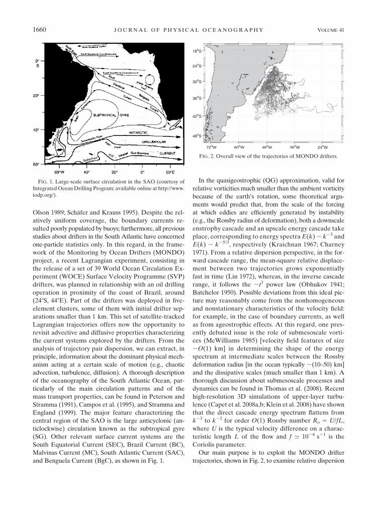
England (1999). The major feature characterizing the

central region of the SAO is the large anticyclonic (an-

ticlockwise) circulation known as the subtropical gyre

(SG). Other relevant surface current systems are the

South Equatorial Current (SEC), Brazil Current (BC),

Malvinas Current (MC), South Atlantic Current (SAC),

and Benguela Current (BgC), as shown in Fig. 1.

In the quasigeostrophic (QG) approximation, valid for

relative vorticities much smaller than the ambient vorticity

because of the earth’s rotation, some theoretical argu-

ments would predict that, from the scale of the forcing

at which eddies are efficiently generated by instability

(e.g., the Rossby radius of deformation), both a downscale

enstrophy cascade and an upscale energy cascade take

place, corresponding to energy spectra E(k) ; k23 and

E(k) ; k25/3, respectively (Kraichnan 1967; Charney

1971). From a relative dispersion perspective, in the for-

ward cascade range, the mean-square relative displace-

ment between two trajectories grows exponentially

fast in time (Lin 1972), whereas, in the inverse cascade

range, it follows the ;t3 power law (Obhukov 1941;

Batchelor 1950). Possible deviations from this ideal pic-

ture may reasonably come from the nonhomogeneous

and nonstationary characteristics of the velocity field:

for example, in the case of boundary currents, as well

as from ageostrophic effects. At this regard, one pres-

ently debated issue is the role of submesoscale vorti-

ces (McWilliams 1985) [velocity field features of size

;O(1) km] in determining the shape of the energy

spectrum at intermediate scales between the Rossby

deformation radius [in the ocean typically ;(10–50) km]

and the dissipative scales (much smaller than 1 km). A

thorough discussion about submesoscale processes and

dynamics can be found in Thomas et al. (2008). Recent

high-resolution 3D simulations of upper-layer turbu-

lence (Capet et al. 2008a,b; Klein et al. 2008) have shown

that the direct cascade energy spectrum flattens from

k23 to k22 for order O(1) Rossby number Ro 5 U/fL,

where U is the typical velocity difference on a charac-

teristic length L of the flow and f ’ 1024 s21 is the

Coriolis parameter.

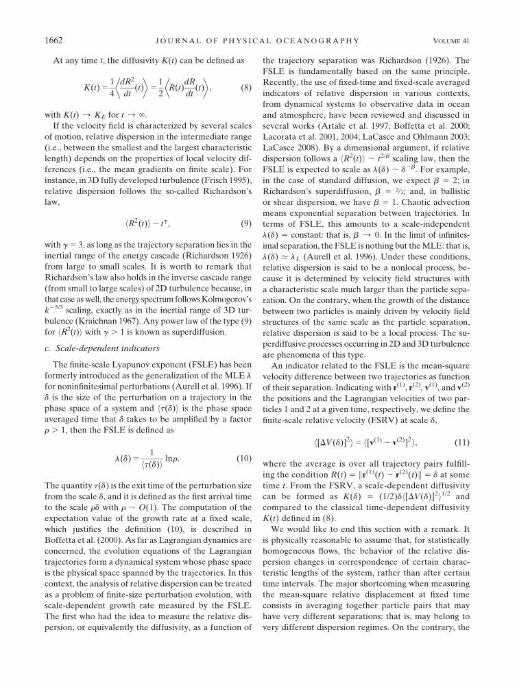
Our main purpose is to exploit the MONDO drifter

trajectories, shown in Fig. 2, to examine relative dispersion

FIG. 1. Large-scale surface circulation in the SAO (courtesy of

Integrated Ocean Drilling Program; available online at http://www.

iodp.org/).

FIG. 2. Overall view of the trajectories of MONDO drifters.

1660 J O U R N A L O F P H Y S I C A L O C E A N O G R A P H Y VOLUME 41

by means of several indicators and discuss the consistency

of our data analysis in comparison with classical turbulence

theory predictions, model simulations and previous drifter

studies available for different regions of the ocean. This

paper is organized as follows: in section 2, we recall the

definitions of the major indicators of the Lagrangian dis-

persion process; in section 3, we give a description of the

MONDO drifter Lagrangian data; in section 4, the out-

come of the data analysis is presented; in section 5, we re-

port the analysis of the ocean model Lagrangian

simulations in comparison with the observative data; and,

in section 6, we outline and discuss the main results we have

obtained in the present work.

2. Lagrangian dispersion indicators

a. One-particle statistics

Let r 5 (x, y, z) be the position vector of a Lagrangian

particle, in a 3D space, evolving according to the equa-

tion dr/dt 5 U(x, y, z, t), where U(x, y, z, t) is a 3D

Eulerian velocity field, and let us indicate with v(t) the

Lagrangian velocity along the trajectory r(t). Let us

imagine, then, a large ensemble of N � 1 Lagrangian

particles, passively advected by the given velocity field,

and refer, for every statistically averaged quantity, to the

mean over the ensemble.

The autocorrelation function of a Lagrangian velocity

component y can be defined, for t1 $ t0, as

C(t1, t0) 5 [hy(t1)y(t0)i2 hy(t0)i2]/[hy(t0)2i2 hy(t0)2i].(1)

In case of stationary statistics, C(t1, t0) depends only on the

time lag t 5 t1 2 t0. The integral Lagrangian time tL is the

time scale after which the autocorrelation has nearly re-

laxed to zero. Typically, tL can be estimated as the time of

the first zero crossing of C(t1, t0) or alternatively as the time

after which jC(t1, t0)j remains smaller than a given threshold.

Absolute dispersion can be defined as the variance of

the particle displacement relatively to the mean position

at time t,

hA2(t)i5 h[r(t) 2 r(0)]2i2 h[r(t) 2 r(0)]i2. (2)

In the limit of very small times, absolute dispersion is

expected to behave as follows:

hA(t)2i ’ s2Lt2, for t� tL, (3)

where tL is the Lagrangian autocorrelation time and s2L

is the total Lagrangian velocity variance. The ballistic

regime (3) lasts as long as the trajectories save some

memory of their initial conditions. In the opposite limit

of very large times, when the autocorrelations have re-

laxed to zero and the memory of the initial conditions is

lost, we have

hA(t)2i ’ 2Kt, for t � tL, (4)

where K is the absolute diffusion coefficient (Taylor

1921).

Although single-particle statistics give information about

the advective transport, mostly because of the largest and

most energetic scales of motion, two (or more) particle

statistics give information about the physical mecha-

nisms acting at any scale of motion, compatibly with the

available resolution.

b. Two-particle statistics

Let us indicate with R(t) 5 kr(1)(t) 2 r(2)(t)k the dis-

tance between two trajectories at time t. Relative dis-

persion is defined as the second-order moment of R(t),

hR2(t)i5 hkr(1)(t) 2 r(2)(t)k2i, (5)

where the average is over all the available trajectory

pairs (r(1), r(2)).

In the small-scale range, the velocity field between

two sufficiently close trajectories is reasonably assumed

to vary smoothly. This means that, in nonlinear flows,

the particle pair separation typically evolves following

an exponential law,

hR2(t)i; eL(2)t, (6)

where, from the theory of dynamical systems, L(2) is the

generalized Lyapunov exponent of order 2 (Bohr et al.

1998). When fluctuations of the finite-time exponential

growth rate around its mean value are weak, one has

L(2) ’ 2lL, where lL is the (Lagrangian) maximum

Lyapunov exponent (MLE; Boffetta et al. 2000). Notice

that, for ergodic trajectory evolutions, the Lyapunov

exponents do not depend on the initial conditions. If

lL . 0 (except for a set of zero probability measure), we

speak of Lagrangian chaos. The chaotic regime holds as

long as the trajectory separation remains sufficiently

smaller than the characteristic scales of motion.

In the opposite limit of large particle separations,

when two trajectories are sufficiently distant from each

other to be considered uncorrelated, the mean-square

relative displacement behaves as

hR2(t)i ’ 4KEt, for t / ‘, (7)

where we indicate with KE the asymptotic eddy-diffusion

coefficient (Richardson 1926).


At any time t, the diffusivity K(t) can be defined as

K(t) 51

4

�dR2

dt(t)

�5

1

2

�R(t)

dR

dt(t)

�, (8)

with K(t) / KE for t / ‘.

If the velocity field is characterized by several scales

of motion, relative dispersion in the intermediate range

(i.e., between the smallest and the largest characteristic

length) depends on the properties of local velocity dif-

ferences (i.e., the mean gradients on finite scale). For

instance, in 3D fully developed turbulence (Frisch 1995),

relative dispersion follows the so-called Richardson’s

law,

hR2(t)i; tg , (9)

with g 5 3, as long as the trajectory separation lies in the

inertial range of the energy cascade (Richardson 1926)

from large to small scales. It is worth to remark that

Richardson’s law also holds in the inverse cascade range

(from small to large scales) of 2D turbulence because, in

that case as well, the energy spectrum follows Kolmogorov’s

k25/3 scaling, exactly as in the inertial range of 3D tur-

bulence (Kraichnan 1967). Any power law of the type (9)

for hR2(t)i with g . 1 is known as superdiffusion.

c. Scale-dependent indicators

The finite-scale Lyapunov exponent (FSLE) has been

formerly introduced as the generalization of the MLE l

for noninfinitesimal perturbations (Aurell et al. 1996). If

d is the size of the perturbation on a trajectory in the

phase space of a system and ht(d)i is the phase space

averaged time that d takes to be amplified by a factor

r . 1, then the FSLE is defined as

l(d) 51

ht(d)i lnr. (10)

The quantity t(d) is the exit time of the perturbation size

from the scale d, and it is defined as the first arrival time

to the scale rd with r ; O(1). The computation of the

expectation value of the growth rate at a fixed scale,

which justifies the definition (10), is described in

Boffetta et al. (2000). As far as Lagrangian dynamics are

concerned, the evolution equations of the Lagrangian

trajectories form a dynamical system whose phase space

is the physical space spanned by the trajectories. In this

context, the analysis of relative dispersion can be treated

as a problem of finite-size perturbation evolution, with

scale-dependent growth rate measured by the FSLE.

The first who had the idea to measure the relative dis-

persion, or equivalently the diffusivity, as a function of

the trajectory separation was Richardson (1926). The

FSLE is fundamentally based on the same principle.

Recently, the use of fixed-time and fixed-scale averaged

indicators of relative dispersion in various contexts,

from dynamical systems to observative data in ocean

and atmosphere, have been reviewed and discussed in

several works (Artale et al. 1997; Boffetta et al. 2000;

Lacorata et al. 2001, 2004; LaCasce and Ohlmann 2003;

LaCasce 2008). By a dimensional argument, if relative

dispersion follows a hR2(t)i ; t2/b scaling law, then the

FSLE is expected to scale as l(d) ; d2b. For example,

in the case of standard diffusion, we expect b 5 2; in

Richardson’s superdiffusion, b 5 2/3; and, in ballistic

or shear dispersion, we have b 5 1. Chaotic advection

means exponential separation between trajectories. In

terms of FSLE, this amounts to a scale-independent

l(d) 5 constant: that is, b / 0. In the limit of infinites-

imal separation, the FSLE is nothing but the MLE: that is,

l(d) ’ lL (Aurell et al. 1996). Under these conditions,

relative dispersion is said to be a nonlocal process, be-

cause it is determined by velocity field structures with

a characteristic scale much larger than the particle sepa-

ration. On the contrary, when the growth of the distance

between two particles is mainly driven by velocity field

structures of the same scale as the particle separation,

relative dispersion is said to be a local process. The su-

perdiffusive processes occurring in 2D and 3D turbulence

are phenomena of this type.

An indicator related to the FSLE is the mean-square

velocity difference between two trajectories as function

of their separation. Indicating with r(1), r(2), v(1), and v(2)

the positions and the Lagrangian velocities of two par-

ticles 1 and 2 at a given time, respectively, we define the

finite-scale relative velocity (FSRV) at scale d,

h[DV(d)]2i5 h[v(1) 2 v(2)]2i, (11)

where the average is over all trajectory pairs fulfill-

ing the condition R(t) 5 kr(1)(t) 2 r(2)(t)k5 d at some

time t. From the FSRV, a scale-dependent diffusivity

can be formed as K(d) 5 (1/2)dh[DV(d)]2i1/2 and

compared to the classical time-dependent diffusivity

K(t) defined in (8).

We would like to end this section with a remark. It

is physically reasonable to assume that, for statistically

homogeneous flows, the behavior of the relative dis-

persion changes in correspondence of certain charac-

teristic lengths of the system, rather than after certain

time intervals. The major shortcoming when measuring

the mean-square relative displacement at fixed time

consists in averaging together particle pairs that may

have very different separations: that is, may belong to

very different dispersion regimes. On the contrary, the


mean dispersion rate at fixed scale or other scale-

dependent related quantities generally have the benefit

of being weakly affected by possible overlap effects.

This is of particular relevance because the presence of

scaling laws in the pre-asymptotic regime raises ques-

tions about the characteristics (e.g., the kinetic energy

spectrum) of the underlying velocity field.

3. Dataset and local oceanography

The MONDO project is a campaign planned by

PROOCEANO for Eni Oil do Brasil to provide un-

restricted access to oceanographic data and subsidize

not only the company’s operational goals but also the

scientific community. The Lagrangian experiment con-

sisted in the deployment of 39 WOCE SVP drifters

(Sybrandy and Niiler 1991) in the surroundings of an

oil drilling operation (248249500S, 438469220W) in prox-

imity of the BC. The drifters are of the holey-sock type,

composed by a surface floater, a tether and a submerged

drogue, following the design criteria proposed by

Sybrandy and Niiler (1991). The drogue length is 6.44 m,

centered at 15 m deep, to represent the first 20-m current

information. The drifters are equipped with a GPS de-

vice and iridium transmission, providing a positioning

accuracy of 7 m and an acquiring rate of 3 h. From the

39 drifters, 14 were deployed individually in a 3-day

frequency and 25 were deployed in clusters of 5, every

12 days. Justification for the 3-day frequency deployment

is based on the 6.5-day energy peak in the wind vari-

ability in the region (Stech and Lorenzetti 1992). Data

used in this study comprehend the period within

21 September 2007–14 November 2008 and passed the

quality control proposed by Hansen and Poulain

(1996) in the Global Drifter Program (GDP) data-

base. High-frequency components have been removed

by applying a Blackman low-pass filter with a window of

15 points (45 h).

The domain explored by the MONDO project drifters

mainly corresponds to that of the BC and to the area

where the southward-flowing BC meets the northward-

flowing MC, forming the BMC, which results in an

eastward current feeding the SAC. BC is a warm western

boundary current, flowing southward and meandering

over the 200-m isobath (Peterson and Stramma 1991;

Lima et al. 1996). As reported by de Castro et al. (2006)

and Garfield (1990), the velocities inside the BC have

values between 25 and 80 cm s21. BC flux increases

with latitude (Assireu 2003; Muller et al. 1998; Gordon

and Greengrove 1986) and veers toward the east when

meeting the colder Malvinas Current around 408S. The

BMC is a highly energetic zone with strong thermal

gradient and great variability, playing an important

role in weather and climate of South America (Legeckis

and Gordon 1982; Pezzi et al. 2005; Piola et al. 2008).

Both BC and BMC show intense mesoscale activity with

eddies detaching from both sides of the flow. Lentini

et al. (2002) used satellite-derived sea surface temper-

ature (SST) to estimate an average of 7 rings per year,

with lifetimes ranging from 11 to 95 days with major

and minor radii of 126 6 50 km and 65 6 22 km, re-

spectively. Assireu (2003) estimates a diffusion coefficient

between 6 3 106 and 9.1 3 107 cm2 s21; a Lagrangian time

scale between 1 and 5 days; and a characteristic (Eulerian)

length scale varying from 19 to 42 km, which agrees with

the meridional variation of the first internal Rossby ra-

dius of deformation in the region (Houry et al. 1987).

Studies addressing the energetics in BC and BMC flows

report great spatial and temporal variability (see, e.g.,

Assireu et al. 2003; Piola et al. 1987; Stevenson 1996) with

EKE varying from 200 to 1200 cm2 s22 and representing

70%–90% of the total kinetic energy (TKE). Recently,

Oliveira et al. (2009) extended the analysis made by Piola

et al. (1987) and suggested that EKE is usually lower than

the mean kinetic energy (MKE) in the BC and always

greater in the BMC.

4. Data analysis

a. Single-particle statistics

From a pre-analysis, we eliminated two drifters that

very soon lost their drogue, so the set of active drifters

is reduced to 37 units. The Lagrangian velocity sta-

tistics, reconstructed along the drifter trajectories by

means of a finite-difference scheme, provides standard

deviations, in the zonal and meridional directions, on

the order of ’25 cm s21, compatible with estimates

obtained from other observative data available for the

same ocean region (Figueroa and Olson 1989; Schafer

and Krauss 1995).

The drifters initially tend to move southward, driven

by the BC; then they are nearly stopped by the BMC;

and last they tend to be transported eastward by the

SAC. The time evolution of the drifter mean position

coordinates in longitude and latitude is shown in Fig. 3.

During the first phase of dispersion, the mean meridio-

nal displacement grows almost linearly southward (BC),

whereas the mean zonal displacement is almost con-

stant; after about 120 days from the release time, the

mean meridional displacement tends to saturate (BMC),

whereas the mean zonal displacement tends to grow

almost linearly eastward (SAC). Given the differences

between BC, BMC, and SAC in terms of energy and

circulation patterns and, in general, between the bound-

ary of the subtropical gyre and its interior, the drifters do


not sample a statistically homogeneous and stationary

domain. To evaluate the Lagrangian autocorrelations,

we divide the trajectory lifetime into time windows of

10-day widths. Then, we compute (1), where mean and

variance of the Lagrangian velocity components are re-

calculated for each window, and then we take the aver-

age, for a fixed time lag t 5 t1 2 t0, over all the windows

for all trajectories. The resulting functions are plotted in

Fig. 4. We notice that, because most of the statistics re-

gards trajectory segments within or near the BC, the

motion is slightly more autocorrelated in the meridional

direction than in the zonal direction. However, the order

of the integral time scale is the same for both compo-

nents. Without discussing the various estimates that can

be evaluated using different criteria, we identify the two

integral time scales around a value tL ’ 5 days, with

a difference between zonal and meridional components

of O(1) days. This implies that, for time lags significantly

larger than tL, the Lagrangian velocities along a trajec-

tory become practically uncorrelated.

Absolute dispersion (i.e., the mean-square fluctuation

around the mean position) for zonal and meridional

coordinates is reported in Fig. 5. In the present work, we

are not interested in reproducing estimates of small-

scale diffusivity, obtained by reconstructing a mean

velocity field, in general not spatially uniform, and cal-

culating the turbulent components from the difference

between the drifter local velocities and the local mean

field. Wherever we speak of diffusion coefficients, re-

ferring to (2) or (5), we mean the effective diffusion

coefficients of ;O(UL), where L and U are determined

by the characteristic size and rotation velocity of the

largest eddies, respectively. Absolute dispersion, being

dominated by the large-scale features of the velocity

field, reflects the anisotropy of the currents encountered

by the drifters. The ballistic dispersion ;t2 scaling is

plotted as reference for autocorrelated motions on time

lags smaller than 10 days. The diffusion ;t scaling is

a good approximation for meridional dispersion on time

lags within 10–60 days, but it is not good for zonal dis-

persion on any time lag. After about 60 days, meridional

dispersion tends to saturate, whereas zonal dispersion

starts growing again as ;t2, likely because on those time

lags, on average, the drifters have reached the BMC,

have stopped their southward meridional run along the

BC, and start moving eastward along the SAC, the natural

consequence of which is the saturation of the meridional

component and a second ballistic (or shear) regime for the

zonal component.

FIG. 3. Mass center coordinates in longitude hui and latitude hfi,averaged over all drifters, as function of the time lag since the re-

lease. The time sampling is Dt 5 1/8 day. Error bars are the standard

deviations of the mean values.

FIG. 4. Lagrangian velocity autocorrelation function for zonal and

meridional components. The time sampling is Dt 5 1/8 day.

FIG. 5. Mean-square drifter displacement from the mass center

position hA2(t)i in zonal and meridional components. The time

sampling is Dt 5 1/8 day.


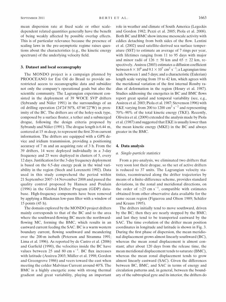
b. Two-particle statistics

Relative dispersion for three different initial separa-

tions is shown in Fig. 6. Distances between two points on

the ocean surface are calculated as great circle arcs,

according to the spherical geometry standard approxi-

mation. A way to increase relative dispersion statistics is

to measure (5) also for so-called chance pairs: that is,

particle pairs that may be initially very distant from each

other but that, following the flow, happen to get suffi-

ciently close to each other at some later time after their

release, in some random point of the domain (LaCasce

2008). The maximum number of pairs counted in the

statistics depends on the initial threshold: 24 pairs for

R(0) # 1 km, 30 pairs for R(0) # 5 km, and 39 pairs for

R(0) # 10 km. The dependence of hR2(t)i on R(0) is well

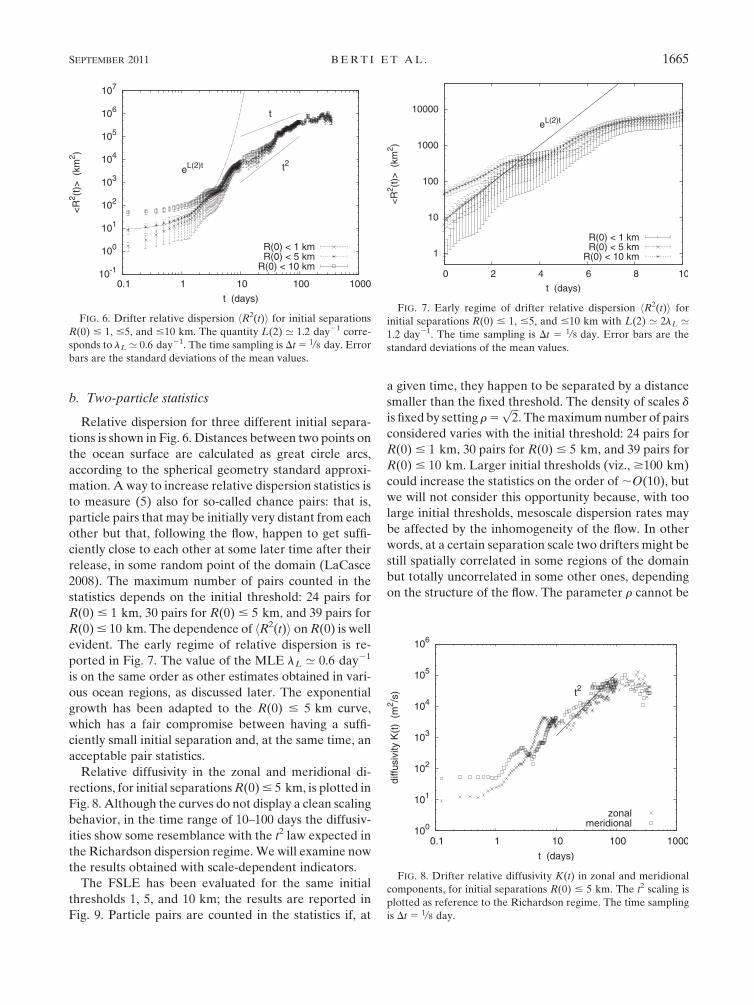
evident. The early regime of relative dispersion is re-

ported in Fig. 7. The value of the MLE lL ’ 0.6 day21

is on the same order as other estimates obtained in vari-

ous ocean regions, as discussed later. The exponential

growth has been adapted to the R(0) # 5 km curve,

which has a fair compromise between having a suffi-

ciently small initial separation and, at the same time, an

acceptable pair statistics.

Relative diffusivity in the zonal and meridional di-

rections, for initial separations R(0) # 5 km, is plotted in

Fig. 8. Although the curves do not display a clean scaling

behavior, in the time range of 10–100 days the diffusiv-

ities show some resemblance with the t2 law expected in

the Richardson dispersion regime. We will examine now

the results obtained with scale-dependent indicators.

The FSLE has been evaluated for the same initial

thresholds 1, 5, and 10 km; the results are reported in

Fig. 9. Particle pairs are counted in the statistics if, at

a given time, they happen to be separated by a distance

smaller than the fixed threshold. The density of scales d

is fixed by setting r 5ffiffiffi2p

. The maximum number of pairs

considered varies with the initial threshold: 24 pairs for

R(0) # 1 km, 30 pairs for R(0) # 5 km, and 39 pairs for

R(0) # 10 km. Larger initial thresholds (viz., $100 km)

could increase the statistics on the order of ;O(10), but

we will not consider this opportunity because, with too

large initial thresholds, mesoscale dispersion rates may

be affected by the inhomogeneity of the flow. In other

words, at a certain separation scale two drifters might be

still spatially correlated in some regions of the domain

but totally uncorrelated in some other ones, depending

on the structure of the flow. The parameter r cannot be

FIG. 6. Drifter relative dispersion hR2(t)i for initial separations

R(0) # 1, #5, and #10 km. The quantity L(2) ’ 1.2 day21 corre-

sponds to lL ’ 0.6 day21. The time sampling is Dt 5 1/8 day. Error

bars are the standard deviations of the mean values.

FIG. 7. Early regime of drifter relative dispersion hR2(t)i for

initial separations R(0) # 1, #5, and #10 km with L(2) ’ 2lL ’1.2 day21. The time sampling is Dt 5 1/8 day. Error bars are the

standard deviations of the mean values.

FIG. 8. Drifter relative diffusivity K(t) in zonal and meridional

components, for initial separations R(0) # 5 km. The t2 scaling is

plotted as reference to the Richardson regime. The time sampling

is Dt 5 1/8 day.


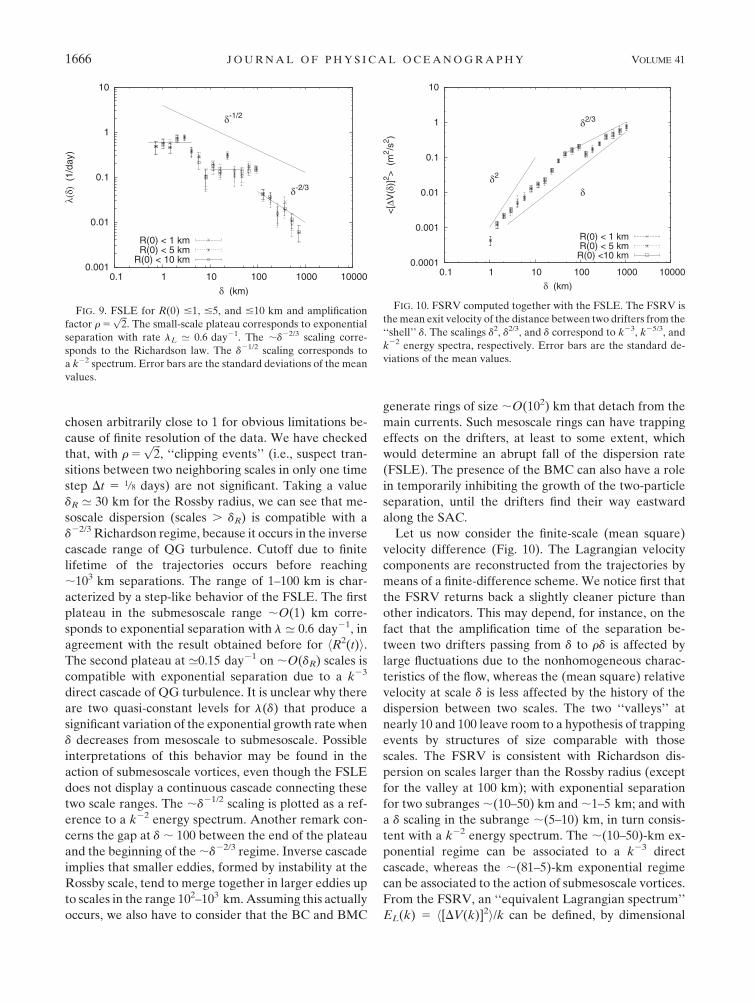
chosen arbitrarily close to 1 for obvious limitations be-

cause of finite resolution of the data. We have checked

that, with r 5ffiffiffi2p

, ‘‘clipping events’’ (i.e., suspect tran-

sitions between two neighboring scales in only one time

step Dt 5 1/8 days) are not significant. Taking a value

dR ’ 30 km for the Rossby radius, we can see that me-

soscale dispersion (scales . dR) is compatible with a

d22/3 Richardson regime, because it occurs in the inverse

cascade range of QG turbulence. Cutoff due to finite

lifetime of the trajectories occurs before reaching

;103 km separations. The range of 1–100 km is char-

acterized by a step-like behavior of the FSLE. The first

plateau in the submesoscale range ;O(1) km corre-

sponds to exponential separation with l ’ 0.6 day21, in

agreement with the result obtained before for hR2(t)i.The second plateau at ’0.15 day21 on ;O(dR) scales is

compatible with exponential separation due to a k23

direct cascade of QG turbulence. It is unclear why there

are two quasi-constant levels for l(d) that produce a

significant variation of the exponential growth rate when

d decreases from mesoscale to submesoscale. Possible

interpretations of this behavior may be found in the

action of submesoscale vortices, even though the FSLE

does not display a continuous cascade connecting these

two scale ranges. The ;d21/2 scaling is plotted as a ref-

erence to a k22 energy spectrum. Another remark con-

cerns the gap at d ; 100 between the end of the plateau

and the beginning of the ;d22/3 regime. Inverse cascade

implies that smaller eddies, formed by instability at the

Rossby scale, tend to merge together in larger eddies up

to scales in the range 102–103 km. Assuming this actually

occurs, we also have to consider that the BC and BMC

generate rings of size ;O(102) km that detach from the

main currents. Such mesoscale rings can have trapping

effects on the drifters, at least to some extent, which

would determine an abrupt fall of the dispersion rate

(FSLE). The presence of the BMC can also have a role

in temporarily inhibiting the growth of the two-particle

separation, until the drifters find their way eastward

along the SAC.

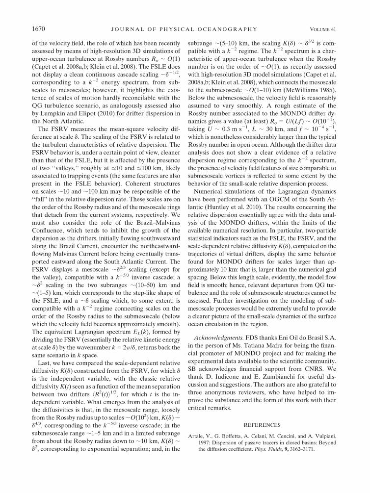
Let us now consider the finite-scale (mean square)

velocity difference (Fig. 10). The Lagrangian velocity

components are reconstructed from the trajectories by

means of a finite-difference scheme. We notice first that

the FSRV returns back a slightly cleaner picture than

other indicators. This may depend, for instance, on the

fact that the amplification time of the separation be-

tween two drifters passing from d to rd is affected by

large fluctuations due to the nonhomogeneous charac-

teristics of the flow, whereas the (mean square) relative

velocity at scale d is less affected by the history of the

dispersion between two scales. The two ‘‘valleys’’ at

nearly 10 and 100 leave room to a hypothesis of trapping

events by structures of size comparable with those

scales. The FSRV is consistent with Richardson dis-

persion on scales larger than the Rossby radius (except

for the valley at 100 km); with exponential separation

for two subranges ;(10–50) km and ;1–5 km; and with

a d scaling in the subrange ;(5–10) km, in turn consis-

tent with a k22 energy spectrum. The ;(10–50)-km ex-

ponential regime can be associated to a k23 direct

cascade, whereas the ;(81–5)-km exponential regime

can be associated to the action of submesoscale vortices.

From the FSRV, an ‘‘equivalent Lagrangian spectrum’’

EL(k) 5 h[DV(k)]2i/k can be defined, by dimensional

FIG. 9. FSLE for R(0) #1, #5, and #10 km and amplification

factor r 5ffiffiffi2p

. The small-scale plateau corresponds to exponential

separation with rate lL ’ 0.6 day21. The ;d22/3 scaling corre-

sponds to the Richardson law. The d21/2 scaling corresponds to

a k22 spectrum. Error bars are the standard deviations of the mean

values.

FIG. 10. FSRV computed together with the FSLE. The FSRV is

the mean exit velocity of the distance between two drifters from the

‘‘shell’’ d. The scalings d2, d2/3, and d correspond to k23, k25/3, and

k22 energy spectra, respectively. Error bars are the standard de-

viations of the mean values.


arguments, replacing d with 2p/k (Fig. 11). The same

scenario formerly indicated by the FSRV is reproduced

in k space by EL(k) as well.

We compare now the diffusivity (see Fig. 12) com-

puted in both ways: as a fixed-time average (8) and as

a fixed-scale average from the FSRV. Both quantities

are plotted as functions of the separation between two

drifters: K(d) 5 (1/2)dh[DV(d)]2i1/2, with d as the in-

dependent variable, and K(t) versus d 5 hR2(t)i1/2,

where the independent variable is the time t. The dif-

fusivity is less affected by distortions present in the

signal than other indicators. The two regimes ;d4/3 at

the mesoscale and ;d2 at a scale ;O(dR) are consistent

with the inverse cascade k25/3 and direct cascade k23,

respectively, as predicted by QG turbulence theory. A

scaling ;d3/2, corresponding to a k22 spectrum, con-

nects scales on the order of the Rossby radius to the

submesoscale, and a scaling ;d2 is the signature of

exponential separation driven by velocity field features

on scales ;O(1) km.

5. Numerical simulations

To check the consistency of the results obtained from

the data analysis of the MONDO drifters, we have

performed two numerical experiments in which ;O(102)

virtual drifters are deployed in a surface current field

generated by a global operational forecast system us-

ing the Hybrid Coordinates Ocean Model (HYCOM;

Bleck and Benjamin 1993) and the Navy Coupled

Ocean Data Assimilation (NCODA; Cummings 2005).

The model grid step is 1/128 (approximately 7 km), and

outputs are available with a 1-day time step. From the

32-layer global grid, the surface layer is extracted in

the area within 458–208S and 608–308S for the same

period of drifters trajectories (20 September 2007–

21 October 2008). Conversion from Earth coordinates

to meters is accomplished following the great circle

distance approximation. The integration algorithm of

the Lagrangian trajectories uses a fixed time step Dt 51/24 day and trilinear interpolations. The maximum in-

tegration time is 400 days, but particles reaching the

shoreline are stopped and removed from the sub-

sequent integration.

We indicate the numerical experiments with E1 and

E2. In the first one (E1), the drifters are uniformly

deployed in an area of about 10 3 10 km2 centered

around a position corresponding to the mean initial lo-

cation of MONDO drifters. The average initial distance

between particle pairs is hR(0)i ’ 5 km. The lifetime of

trajectories is between 150 and 200 days. In the second

experiment (E2), the initial distribution of the drifters

is characterized by larger separations: namely, compa-

rable to the spacing of the numerical grid (;10 km).

The average initial distance between particle pairs

is hR(0)i ’ 40 km, and the duration of trajectories is

250–400 days.

Here, we present some comparisons between the anal-

ysis of data from model trajectories and those from

the actual drifters, focusing on the relative dispersion

process. First, we consider a fixed-time indicator [viz.,

relative dispersion hR2(t)i] for trajectories selected

with small enough initial separation: that is, for R(0) ,

10 km. As can be seen in Fig. 13, the model outcome

is in reasonable agreement with the behavior of ac-

tual drifters. In particular, experiment E1 is capable of

FIG. 11. Equivalent Lagrangian spectrum defined from the FSRV.

The inverse cascade (k25/3), direct cascade (k23), and submesoscale

(k22) spectra are plotted as reference. The Rossby radius ’ 30 km

corresponds to a wavenumber k ’ 0.2.

FIG. 12. Diffusivity as a function of the separation: fixed-time

average K(t) vs d 5 hR2(t)i1/2 and fixed-scale average K(d) vs d. The

d4/3 and d2 correspond to k25/3 and k23 spectra, respectively. The d3/2

scaling corresponds to a k22 spectrum.


reproducing the early growth of relative dispersion,

but it cannot catch the late time behavior because of

too short trajectories. On the other hand, with ex-

periment E2 we obtain a nicer agreement at late times,

thanks to the longer lifetime of virtual trajectories in

this case, but we lose the agreement at early times

because now the initial separation between particle

pairs is on average much larger.

For what concerns fixed-scale indicators, we consider

the FSLE and FSRV (Figs. 14, 15). To increase the

statistics, we now select trajectories with a larger initial

separation: that is, for R(0) , 50 km [similar results are

found for smaller values of R(0), though they are more

noisy]. The behaviors of both FSLE and FSRV support

a double-cascade scenario on the same scales as those

found with MONDO drifters. The plateau value of

FSLE at scales O(dR) is very close to the one found in

the real experiment (l ’ 0.15 day21). At larger scales,

for both numerical experiments E1 and E2, the behavior

of FSLE is compatible with a scaling law l(d) ; d22/3

supporting an inverse energy cascade process. Experi-

ment E2, which is characterized by longer trajectories,

shows a clearer scaling, thanks to a larger number of

pairs reaching this range of large scales. Mean-square

velocity differences in the same range of scales display

a reasonably clear d2/3 scaling, also supporting an inverse

energy cascade, with values close to those found with

MONDO drifters. At separations smaller than the

Rossby deformation radius, both indicators point to the

presence of a direct enstrophy cascade: the FSLE is

constant and the FSRV behaves as h[DV(d)]2i; d2. This

only partially agrees with the results found for real

drifters: namely, only in the scale range 10 km , d ,

50 km. At subgrid scales, velocity field features are not

resolved and relative dispersion is necessarily a nonlocal

exponential process driven by structures of size on the

order of (at least) the Rossby radius. Correspondingly,

the FSLE computed on model trajectories does not

display the higher plateau level at scales smaller than

10 km.

Finally, the behavior of the relative diffusivity K(d) as

a function of the separation d is shown in Fig. 16 for both

MONDO and virtual drifters. Here, K(d) is computed

from the mean-square velocity difference, as described

in sections 2c and 4b. Model and experimental data again

are in agreement at scales larger than the numerical space

resolution (;10 km). Indeed, in both numerical experi-

ments E1 and E2, we find scaling behaviors compatible

with a QG double cascade: K(d) ; d4/3 (corresponding to

FIG. 13. Relative dispersion hR2(t)i for initial separations R(0) #

10 km for MONDO drifters and virtual drifters from numerical

experiments E1 and E2. For virtual drifters, errors are on the order

of point size; time sampling is Dt 5 1/8 day for MONDO drifters

and Dt 5 1/24 day for virtual drifters.

FIG. 14. FSLE for R(0) # 50 km and amplification factor r 5ffiffiffi2p

for MONDO drifters and virtual drifters from numerical experi-

ments E1 and E2. For virtual drifters, errors are on the order of

point size. The large-scale saturation (E1) depends on the value of

the trajectory integration time.

FIG. 15. FSRV for R(0) # 50 km for MONDO drifters and vir-

tual drifters from numerical experiments E1 and E2. For virtual

drifters, errors are on the order of point size.


Richardson’s superdiffusion in an inverse cascade re-

gime) for d . dR and K(d) ; d2 (corresponding to a direct

cascade smooth flow) for d , dR. At variance with the

outcome of the real experiment with MONDO drifters,

here we are unable to detect any significant deviations

from the QG turbulence scenario at small scales.

The failure of the model to reproduce flow features at

very small scales is of course due to its finite spatial

resolution, which is on the order of 10 km. Below this

length scale, the velocity field computed in the model is

smooth, whereas the one measured in the real ocean

clearly displays active scales also in the range of 1–10 km.

Nevertheless, the overall conclusion we can draw from

the above comparisons is that the characteristics of the

relative dispersion process found with MONDO drifters

agree with those obtained with an ocean general circula-

tion model (OGCM) for scales d . 10 km.

6. Discussion and conclusions

Lagrangian dispersion properties of drifters launched

in the southwestern corner of the South Atlantic sub-

tropical gyre have been analyzed through the computa-

tion of time-dependent and scale-dependent indicators.

The data come from a set of 39 WOCE–SVP drifters

deployed in the Brazil Current around (248S, 448S) during

the Monitoring by Ocean Drifters (MONDO) project, an

oceanographic campaign planned by PROOCEANO and

supported by Eni Oil do Brasil in relationship with an oil

drilling operation. The experimental strategy of deploying

part of the drifters in five-element clusters, with initial

separation between drifters smaller than 1 km, allows us to

study relative dispersion on a wide range of scales.

Single-particle analysis has been performed by com-

puting classic quantities like Lagrangian autocorrelation

functions and absolute dispersion, defined as the vari-

ance around the drifter mean position, as a function

of the time lag from the release. Velocity variances

(;500 cm2 s22) and integral time scales (tL ; 5 days)

are compatible with the estimates obtained in the

analysis of the FGGE drifters (Figueroa and Olson

1989; Schafer and Krauss 1995). Anisotropy of the flow

is reflected in the different behavior of the zonal and

meridional components of the absolute dispersion.

Being the MONDO drifters advected mostly by the

boundary currents surrounding the subtropical gyre,

the Brazil Current first and the South Atlantic Current

later, the meridional component of the absolute dis-

persion is dominant as long as the mean drifter di-

rection is nearly southward (BC), whereas the zonal

component dominates (see the appearance of the late

ballistic regime) as the mean drifter direction is nearly

eastward (SAC). Early time advection is modulated

also by the response of the currents to a wind forcing of

period ;6.5 days, a characteristic meteorological fea-

ture of the BC dynamics.

Two-particle analysis has been performed by means

of both fixed-time and fixed-scale averaged quantities.

Classic indicators like the mean-square relative dis-

placement and the relative diffusivities between two

drifters as functions of the time lag from the release give

loose information about early phase exponential sepa-

ration, characterized by a mean rate lL’ 0.6 day21, and

longtime dispersion approximated, to some extent, by

Richardson superdiffusion before the cutoff due to the

finite lifetime of the trajectories. Evidence of a small-

scale exponential regime for relative dispersion is com-

mon to other drifter studies for different ocean regions

(LaCasce and Ohlmann 2003; Ollitrault et al. 2005;

Koszalka et al. 2009; Lumpkin and Elipot 2010). Scale-

dependent indicators return back a cleaner picture,

compatibly with the limited statistics allowed by the

experimental data and the nonhomogeneous and non-

stationary characteristics of the flow.

The FSLE displays a mesoscale (100–500 km) regime

compatible with Richardson superdiffusion, with the

Lagrangian counterpart of the 2D inverse cascade sce-

nario characterized by a k25/3 energy spectrum. At

scales smaller than 100 km, the FSLE has a step-like

shape, with a first plateau at level ;0.6 day21 in the

submesoscale range ;O(1) km and a second plateau

at level ’0.15 day21 for scales comparable with the

Rossby radius of deformation (dR ’ 30 km). Constant

FSLE in a range of scales corresponds to exponential

separation. The ;O(dR) plateau could be related to the

2D direct cascade characterized by a k23 energy spec-

trum, whereas the origin of the ;O(1) km plateau is

likely related to the existence of submesoscale features

FIG. 16. Diffusivity K(d) as function of the separation d for

MONDO drifters and virtual drifters from numerical experiments

E1 and E2; here, R(0) , 50 km.


of the velocity field, the role of which has been recently

assessed by means of high-resolution 3D simulations of

upper-ocean turbulence at Rossby numbers Ro ; O(1)

(Capet et al. 2008a,b; Klein et al. 2008). The FSLE does

not display a clean continuous cascade scaling ;d21/2,

corresponding to a k22 energy spectrum, from sub-

scales to mesoscales; however, it highlights the exis-

tence of scales of motion hardly reconcilable with the

QG turbulence scenario, as analogously assessed also

by Lumpkin and Elipot (2010) for drifter dispersion in

the North Atlantic.

The FSRV measures the mean-square velocity dif-

ference at scale d. The scaling of the FSRV is related to

the turbulent characteristics of relative dispersion. The

FSRV behavior is, under a certain point of view, cleaner

than that of the FSLE, but it is affected by the presence

of two ‘‘valleys,’’ roughly at ’10 and ’100 km, likely

associated to trapping events (the same features are also

present in the FSLE behavior). Coherent structures

on scales ;10 and ;100 km may be responsible of the

‘‘fall’’ in the relative dispersion rate. These scales are on

the order of the Rossby radius and of the mesoscale rings

that detach from the current systems, respectively. We

must also consider the role of the Brazil–Malvinas

Confluence, which tends to inhibit the growth of the

dispersion as the drifters, initially flowing southwestward

along the Brazil Current, encounter the northeastward-

flowing Malvinas Current before being eventually trans-

ported eastward along the South Atlantic Current. The

FSRV displays a mesoscale ;d2/3 scaling (except for

the valley), compatible with a k25/3 inverse cascade; a

;d2 scaling in the two subranges ;(10–50) km and

;(1–5) km, which corresponds to the step-like shape of

the FSLE; and a ;d scaling which, to some extent, is

compatible with a k22 regime connecting scales on the

order of the Rossby radius to the submesoscale (below

which the velocity field becomes approximately smooth).

The equivalent Lagrangian spectrum EL(k), formed by

dividing the FSRV (essentially the relative kinetic energy

at scale d) by the wavenumber k 5 2p/d, returns back the

same scenario in k space.

Last, we have compared the scale-dependent relative

diffusivity K(d) constructed from the FSRV, for which d

is the independent variable, with the classic relative

diffusivity K(t) seen as a function of the mean separation

between two drifters hR2(t)i1/2, for which t is the in-

dependent variable. What emerges from the analysis of

the diffusivities is that, in the mesoscale range, loosely

from the Rossby radius up to scales ;O(102) km, K(d) ;

d4/3, corresponding to the k25/3 inverse cascade; in the

submesoscale range ;1–5 km and in a limited subrange

from about the Rossby radius down to ;10 km, K(d) ;

d2, corresponding to exponential separation; and, in the

subrange ;(5–10) km, the scaling K(d) ; d3/2 is com-

patible with a k22 regime. The k22 spectrum is a char-

acteristic of upper-ocean turbulence when the Rossby

number is on the order of ;O(1), as recently assessed

with high-resolution 3D model simulations (Capet et al.

2008a,b; Klein et al. 2008), which connects the mesoscale

to the submesoscale ;O(1–10) km (McWilliams 1985).

Below the submesoscale, the velocity field is reasonably

assumed to vary smoothly. A rough estimate of the

Rossby number associated to the MONDO drifter dy-

namics gives a value (at least) Ro 5 U/(Lf) ; O(1021),

taking U ; 0.3 m s21, L ; 30 km, and f ; 1024 s21,

which is nonetheless considerably larger than the typical

Rossby number in open ocean. Although the drifter data

analysis does not show a clear evidence of a relative

dispersion regime corresponding to the k22 spectrum,

the presence of velocity field features of size comparable to

submesoscale vortices is reflected to some extent by the

behavior of the small-scale relative dispersion process.

Numerical simulations of the Lagrangian dynamics

have been performed with an OGCM of the South At-

lantic (Huntley et al. 2010). The results concerning the

relative dispersion essentially agree with the data anal-

ysis of the MONDO drifters, within the limits of the

available numerical resolution. In particular, two-particle

statistical indicators such as the FSLE, the FSRV, and the

scale-dependent relative diffusivity K(d), computed on the

trajectories of virtual drifters, display the same behavior

found for MONDO drifters for scales larger than ap-

proximately 10 km: that is, larger than the numerical grid

spacing. Below this length scale, evidently, the model flow

field is smooth; hence, relevant departures from QG tur-

bulence and the role of submesoscale structures cannot be

assessed. Further investigation on the modeling of sub-

mesoscale processes would be extremely useful to provide

a clearer picture of the small-scale dynamics of the surface

ocean circulation in the region.

Acknowledgments. FDS thanks Eni Oil do Brasil S.A.

in the person of Ms. Tatiana Mafra for being the finan-

cial promoter of MONDO project and for making the

experimental data available to the scientific community.

SB acknowledges financial support from CNRS. We

thank D. Iudicone and E. Zambianchi for useful dis-

cussion and suggestions. The authors are also grateful to

three anonymous reviewers, who have helped to im-

prove the substance and the form of this work with their

critical remarks.

REFERENCES

Artale, V., G. Boffetta, A. Celani, M. Cencini, and A. Vulpiani,

1997: Dispersion of passive tracers in closed basins: Beyond

the diffusion coefficient. Phys. Fluids, 9, 3162–3171.


Assireu, A. T., 2003: Estudo das caracterısticas cinematicas e di-

namicas das aguas de superfıcie do Atlantico Sul Ocidental

a partir de derivadores rastreados por satelite. Ph.D. thesis,

Instituto Nacional de Pesquisas Espaciais, 154 pp.

——, M. Stevenson, and J. Stech, 2003: Surface circulation and

kinetic energy in the SW Atlantic obtained by drifters. Cont.

Shelf Res., 23, 145–157.

Aurell, E., G. Boffetta, A. Crisanti, G. Paladin, and A. Vulpiani,

1996: Growth of non-infinitesimal perturbations in turbulence.

Phys. Rev. Lett., 77, 1262–1265.

Batchelor, G. K., 1950: The application of the similarity theory of

turbulence to atmospheric diffusion. Quart. J. Roy. Meteor.

Soc., 76, 133–146.

Bleck, R., and S. Benjamin, 1993: Regional weather prediction

with a model combining terrain-following and isentropic

coordinates. Part I: Model description. Mon. Wea. Rev., 121,

1770–1785.

Boffetta, G., A. Celani, M. Cencini, G. Lacorata, and A. Vulpiani,

2000: Non-asymptotic properties of transport and mixing.

Chaos, 10, 50–60.

Bohr, T., M. H. Jensen, G. Paladin, and A. Vulpiani, 1998: Dy-

namical Systems Approach to Turbulence. Cambridge Uni-

versity Press, 350 pp.

Campos, E. J. D., J. L. Miller, T. J. Muller, and R. G. Peterson,

1995: Physical oceanography of the southwest Atlantic Ocean.

Oceanography, 8, 87–91.

Capet, X., J. C. McWilliams, M. J. Molemaker, and A. F. Shchepetkin,

2008a: Mesoscale to submesoscale transition in the California

Current System. Part I: Flow structure, eddy flux, and ob-

servational tests. J. Phys. Oceanogr., 38, 29–43.

——, ——, ——, and ——, 2008b: Mesoscale to submesoscale

transition in the California Current System. Part II: Frontal

processes. J. Phys. Oceanogr., 38, 44–64.

Charney, J. G., 1971: Geostrophic turbulence. J. Atmos. Sci., 28,

1087–1094.

Cummings, J. A., 2005: Operational multivariate ocean data as-

similation. Quart. J. Roy. Meteor. Soc., 131, 3583–3604.

de Castro, B. M., J. A. Lorenzetti, I. C. A. da Silveira, and L. B.

de Miranda, 2006: Estrutura termohalina e circulacao

na regiao entre o Cabo de Sao Tome (RJ) e o Chuı (RS).

O Ambiente Oceanografico da Plataforma Continental e

do Talude na Regiao Sudeste-Sul do Brasil, C. L. D. B.

Rossi-Wongtschowski and L. S.-P. Madureira, Eds., Edusp,

11–120.

Figueroa, H. A., and D. B. Olson, 1989: Lagrangian statistics in

the South Atlantic as derived from SOS and FGGE drifters.

J. Mar. Res., 47, 525–546.

Frisch, U., 1995: Turbulence: The Legacy of A. N. Kolmogorov.

Cambridge University Press, 296 pp.

Garfield, N., 1990: The Brazil Current at subtropical latitudes.

Ph.D. thesis, University of Rhode Island, 122 pp.

Gordon, A., and C. Greengrove, 1986: Geostrophic circulation

of the Brazil-Falkland confluence. Deep-Sea Res., 33A,

573–585.

Hansen, D. V., and P. M. Poulain, 1996: Quality control and in-

terpolations of WOCE–TOGA drifter data. J. Atmos. Oceanic

Technol., 13, 900–909.

Houry, S., E. Dombrowsky, P. D. Mey, and J. Minster, 1987: Brunt-

Vaisala frequency and Rossby radii in the South Atlantic.

J. Phys. Oceanogr., 17, 1619–1626.

Huntley, H. S., B. L. Lipphardt Jr., and A. D. Kirwan Jr., 2010:

Lagrangian predictability assessed in the East China Sea. Ocean

Modell., 36, 163–178, doi:10.1016/j.ocemod.2010.11.001.

Klein, P., B. L. Hua, G. Lapeyre, X. Capet, S. L. Gentil, and

H. Sasaki, 2008: Upper ocean turbulence from high-resolution

3D simulations. J. Phys. Oceanogr., 38, 1748–1763.

Koszalka, I., J. H. LaCasce, and K. A. Orvik, 2009: Relative dis-

persion in the Nordic Seas. J. Mar. Res., 67, 411–433.

Kraichnan, R. H., 1967: Inertial ranges in two-dimensional turbu-

lence. Phys. Fluids, 10, 1417–1423.

LaCasce, J. H., 2008: Statistics from Lagrangian observations.

Prog. Oceanogr., 77, 1–29.

——, and C. Ohlmann, 2003: Relative dispersion at the surface of

the Gulf of Mexico. J. Mar. Res., 61, 285–312.

Lacorata, G., E. Aurell, and A. Vulpiani, 2001: Drifter dispersion

in the Adriatic Sea: Lagrangian data and chaotic model. Ann.

Geophys., 19, 121–129.

——, ——, B. Legras, and A. Vulpiani, 2004: Evidence for a k25/3

spectrum from the EOLE Lagrangian balloons in the low

stratosphere. J. Atmos. Sci., 61, 2936–2942.

Legeckis, R., and A. Gordon, 1982: Satellite observations of the

Brazil and Falkland currents 1975 to 1976 and 1978. Deep-Sea

Res., 29, 375–401.

Lentini, C., D. Olson, and G. Podesta, 2002: Statistics of Brazil

Current rings observed from AVHRR: 1993 to 1998. Geophys.

Res. Lett., 29, 1811.

Lima, I. D., C. A. E. Garcia, and O. O. Moller, 1996: Ocean

surface processes on the southern Brazilian shelf: Charac-

terization and seasonal variability. Cont. Shelf Res., 16,

1307–1317.

Lin, J. T., 1972: Relative dispersion in the enstrophy-cascading

inertial range of homogeneous two-dimensional turbulence.

J. Atmos. Sci., 29, 394–395.

Lumpkin, R., and S. Elipot, 2010: Surface drifter pair spreading in

the North Atlantic. J. Geophys. Res., 115, C12017, doi:10.1029/

2010JC006338.

McWilliams, J. C., 1985: Submesoscale, coherent vortices in the

ocean. Rev. Geophys., 23, 165–182.

Muller, T. J., Y. Ikeda, N. Zangenberg, and L. V. Nonato, 1998:

Direct measurements of western boundary currents off

Brazil between 208S and 288S. J. Geophys. Res., 103 (C3),

5429–5437.

Obhukov, A. M., 1941: Energy distribution in the spectrum

of turbulent flow. Izv. Akad. Nauk SSSR, Ser. Geofiz., 5,

453–466.

Oliveira, L. R., A. R. Piola, M. M. Mata, and I. D. Soares, 2009:

Brazil Current surface circulation and energetics observed from

drifting buoys. J. Geophys. Res., 114, C10006, doi:10.1029/

2008JC004900.

Ollitrault, M., C. Gabillet, and A. C. D. Verdiere, 2005: Open

ocean regimes of relative dispersion. J. Fluid Mech., 533,

381–407.

Peterson, R. G., and L. Stramma, 1991: Upper-level circulation in

the South Atlantic Ocean. Prog. Oceanogr., 26, 1–73.

Pezzi, L. P., R. B. Souza, M. S. Dourado, C. A. E. Garcia, M. M.

Mata, and M. A. F. Silva-Dias, 2005: Ocean-atmosphere in situ

observations at the Brazil-Malvinas Confluence region. Geo-

phys. Res. Lett., 32, L22603, doi:10.1029/2005GL023866.

Piola, A. R., H. A. Figueroa, and A. A. Bianchi, 1987: Some aspects

of the surface circulation south of 208S revealed by first GARP

global experiment drifters. J. Geophys. Res., 92 (C5), 5101–

5114.

——, O. O. Moller, R. A. Guerrero, and E. J. D. Campos, 2008:

Variability of the subtropical shelf front off eastern South

America: Winter 2003 and summer 2004. Cont. Shelf Res., 28,

1639–1648.


Richardson, L. F., 1926: Atmospheric diffusion shown on a distance-

neighbor graph. Proc. Roy. Soc. London, 110A, 709–737.

Schafer, H., and W. Krauss, 1995: Eddy statistics in the South At-

lantic as derived from drifters drogued at 100 m. J. Mar. Res.,

53, 403–431.

Stech, J., and J. Lorenzetti, 1992: The response of the South Brazil

Bight to the passage of wintertime cold fronts. J. Geophys.

Res., 97 (C6), 9507–9520.

Stevenson, M. R., 1996: Recirculation of the Brazil Current south

of 238S. WOCE International Newsletter, No. 22, WOCE In-

ternational Project Office, Southampton, United Kingdom,

30–32.

Stramma, L., and M. England, 1999: On the water masses and mean

circulation of the South Atlantic Ocean. J. Geophys. Res., 104

(C9), 20 863–20 883.

Sybrandy, A. L., and P. P. Niiler, 1991: WOCE/TOGA SVP La-

grangian drifter construction manual. Scripps Institution of

Oceanography Rep. 91/6, 58 pp.

Taylor, G. I., 1921: Diffusion by continuous movements. Proc.

London Math. Soc., 20, 196–212.

Thomas, L. N., A. Tandon, and A. Mahadevan, 2008: Sub-

mesoscale processes and dynamics. Eddy Resolving Ocean

Modeling, M. W. Hecht and H. Hasumi, Eds., Amer. Geophys.

Union, 17–38.


lagrangian drifter dispersion in the southwestern atlantic ... · lagrangian drifter dispersion in...

Documents