1

Name: SOLUTION (Havlicek)

Section:

Laboratory Exercise 5

DIGITAL PROCESSING OF CONTINUOUS-TIME SIGNALS

5.1 THE SAMPLING PROCESS IN THE TIME-DOMAIN

Project 5.1 Sampling of a Sinusoidal Signal

A copy of Program P5_1 is given below: % Program P5_1 % Illustration of the Sampling Process % in the Time-Domain clf; t = 0:0.0005:1; f = 13; xa = cos(2*pi*f*t); subplot(2,1,1) plot(t,xa);grid xlabel('Time, msec');ylabel('Amplitude'); title('Continuous-time signal x_{a}(t)'); axis([0 1 -1.2 1.2]) subplot(2,1,2); T = 0.1; n = 0:T:1; xs = cos(2*pi*f*n); k = 0:length(n)-1; stem(k,xs);grid; xlabel('Time index n');ylabel('Amplitude'); title('Discrete-time signal x[n]'); axis([0 (length(n)-1) -1.2 1.2])

2

Answers:

Q5.1 The plots of the continuous-time signal and its sampled version generated by running Program P5_1 are shown below:

0 0.1 0.2 0.3 0.4 0.5 0.6 0.7 0.8 0.9 1

-1

-0.5

0

0.5

1

Time, msec

Am

plitu

de

Continuous-time signal xa(t)

0 1 2 3 4 5 6 7 8 9 10

-1

-0.5

0

0.5

1

Time index n

Am

plitu

de

Discrete-time signal x[n]

Q5.2 The frequency of the sinusoidal signal in Hz is – f = 13 kHz. This is because the time scale shown in the upper graph is in msec. Thus, the sinusoid goes through 13 cycles in 1 msec, or 13,000 cycles in one sec.

The sampling period in seconds is - T = 0.1 msec.

Q5.3 The effects of the two axis commands are – The first axis command sets the minimum and maximum values for the x-axis and the y-axis in the upper plot. The second axis command does the same thing for the lower plot. In each axis command, the first two parameters are the minimum and maximum values for the x-axis. The third and fourth parameters are the minimum and maximum values for the y-axis.

Q5.4 The plots of the continuous-time signal and its sampled version generated by running Program P5_1 for the following four values of the sampling period are shown below:

3

T = 0.004 msec

0 0.1 0.2 0.3 0.4 0.5 0.6 0.7 0.8 0.9 1

-1

-0.5

0

0.5

1

Time, msec

Am

plitu

de

Continuous-time signal xa(t)

0 50 100 150 200 250

-1

-0.5

0

0.5

1

Time index n

Am

plitu

de

Discrete-time signal x[n]

T = 0.02 msec

0 0.1 0.2 0.3 0.4 0.5 0.6 0.7 0.8 0.9 1

-1

-0.5

0

0.5

1

Time, msec

Am

plitu

de

Continuous-time signal xa(t)

0 5 10 15 20 25 30 35 40 45 50

-1

-0.5

0

0.5

1

Time index n

Am

plitu

de

Discrete-time signal x[n]

4

T = 0.15 msec

0 0.1 0.2 0.3 0.4 0.5 0.6 0.7 0.8 0.9 1

-1

-0.5

0

0.5

1

Time, msec

Am

plitu

de

Continuous-time signal xa(t)

0 1 2 3 4 5 6

-1

-0.5

0

0.5

1

Time index n

Am

plitu

de

Discrete-time signal x[n]

T = 0.2 msec

0 0.1 0.2 0.3 0.4 0.5 0.6 0.7 0.8 0.9 1

-1

-0.5

0

0.5

1

Time, msec

Am

plitu

de

Continuous-time signal xa(t)

0 0.5 1 1.5 2 2.5 3 3.5 4 4.5 5

-1

-0.5

0

0.5

1

Time index n

Am

plitu

de

Discrete-time signal x[n]

5

Based on these results we make the following observations – Since the “analog” waveform goes through 13 cycles in the 1 msec shown in the graph, there will be aliasing unless we get at least two samples per cycle, or 26 samples total on the graph. 26 samples in 1

msec is a sampling rate of 26 kHz, which requires T < 1/26 » 0.0385 msec to avoid

aliasing. With T=0.004 msec. there is no aliasing and the discrete-time waveform has an appearance that is very similar to that of the “analog” waveform. With T=0.02 msec, there is still no aliasing, but the sampling rate is much closer to being “critical,” i.e., much closer to the Nyquist rate. Consequently, the appearance of the discrete-time waveform is less similar to the “analog waveform,” although perfect reconstruction is still possible. With T=0.15 msec, there is significant aliasing and the discrete-time waveform has the appearance of an “analog” waveform of much lower frequency. Finally, with T=0.2 msec, there is again severe aliasing which causes the discrete-time waveform to have the appearance of an “analog” waveform of lower frequency.

Q5.5 The plots of the continuous-time sinusoidal signal of frequency 3 kHz and its sampled version generated by running a modified Program P5_1 are shown below: (NOTE: the book is in error about the frequency. Since the “t” in the program is in units of msec, the frequency here is 3 kHz, not 3 Hz.)

0 0.1 0.2 0.3 0.4 0.5 0.6 0.7 0.8 0.9 1

-1

-0.5

0

0.5

1

Time, msec

Am

plitu

de

Continuous-time signal xa(t)

0 1 2 3 4 5 6 7 8 9 10

-1

-0.5

0

0.5

1

Time index n

Am

plitu

de

Discrete-time signal x[n]

6

The plots of the continuous-time sinusoidal signal of frequency 7 kHz and its sampled version generated by running a modified Program P5_1 are shown below: (Again, the book is in error. For the same reason as above, the frequency here is 7 kHz, not 7 Hz.)

0 0.1 0.2 0.3 0.4 0.5 0.6 0.7 0.8 0.9 1

-1

-0.5

0

0.5

1

Time, msec

Am

plitu

de

Continuous-time signal xa(t)

0 1 2 3 4 5 6 7 8 9 10

-1

-0.5

0

0.5

1

Time index n

Am

plitu

de

Discrete-time signal x[n]

Based on these results we make the following observations – In all three cases, we have T = 0.1 msec. Originally, in Q5.1. we had f = 13kHz. This gives a maximum sampling

period of 1/26 » 0.0385 msec to satisfy the Nyquist criterion, as we observed above.

Since 0.1 > 1/26, the Nyquist criterion is not satisfied and there is aliasing in the original discrete-time waveform of Q5.1. In Q5.5 with f = 3 kHz, the maximum

sampling period that satisfies the Nyquist criterion is 1/6 » 0.1667 msec, Therefore,

with T = 0.1 msec we obtain a discrete-time waveform that is not aliased. Finally, in

Q5.5 with f = 7 kHz, the maximum sampling period to avoid aliasing is 1/14 » 0.0714

msec. Thus, with T = 0.1 msec there is aliasing in the discrete-time waveform, but it is not as severe as what we saw above when f = 13 kHz. Interestingly, the samples x[n] are exactly the same in all three cases!

7

Project 5.2 Aliasing Effect in the Time-Domain

A copy of Program P5_2 is given below: % Program P5_2 % Illustration of Aliasing Effect in the Time-Domain % Program adapted from [Kra94] with permission from % The Mathworks, Inc., Natick, MA. clf; T = 0.1;f = 13; n = (0:T:1)'; xs = cos(2*pi*f*n); t = linspace(-0.5,1.5,500)'; ya = sinc((1/T)*t(:,ones(size(n))) - (1/T)*n(:,ones(size(t)))')*xs; plot(n,xs,'o',t,ya);grid; xlabel('Time, msec');ylabel('Amplitude'); title('Reconstructed continuous-time signal y_{a}(t)'); axis([0 1 -1.2 1.2]); Answers:

Q5.6 The plots of the discrete-time signal and its continuous-time equivalent obtained by running Program P5_2 are shown below:

0 0.1 0.2 0.3 0.4 0.5 0.6 0.7 0.8 0.9 1

-1

-0.8

-0.6

-0.4

-0.2

0

0.2

0.4

0.6

0.8

1

Time, msec

Am

plitu

de

Reconstructed continuous-time signal ya(t)

Q5.7 The range of t in the Program is - 0.5 1.5t− ≤ ≤

The value of the time increment is – 0.004

The range of t in the plot is - 0.0 1.0t≤ ≤

8

The plot generated by running Program P5_2 again with the range of t changed so as to display the full range of ya(t) is shown below:

-0.5 0 0.5 1 1.5

-1

-0.8

-0.6

-0.4

-0.2

0

0.2

0.4

0.6

0.8

1

Time, msec

Am

plitu

de

Reconstructed continuous-time signal ya(t)

Based on these results we make the following observations – To understand what is going on, the important line of the program is line 10, which reads:

ya = sinc((1/T)*t(:,ones(size(n))) - (1/T)*n(:,ones(size(t)))')*xs;

Here, t(:,ones(size(n))) is a matrix. It has one column for each element of the vector “n.” Each column contains a copy of the entire vector “t.” Similarly, n(:,ones(size(t)))' is a matrix that has one row for each each entry in the vector “t.” Each one of these rows contains a copy of the vector “n”. It is important to realize that the vector “n” does not actually contain integers as you might expect. What it actually contains are the values nT, i.e., it contains integer multiples of the sampling interval. So the quantity t(:,ones(size(n))) - n(:,ones(size(t)))' is a matrix that has one row for each element of the vector “t” and one column for each element of the vector “n.” The argument of “sinc” in line 10 of the program is this matrix times 1/T. That is a matrix where the first row is exactly the values (t-nT)/T shown on page 73 of the Lab Manual in the sum of Eq. (5.14) when t is the first entry in the vector “t” and n ranges not from −∞ to ∞ , but rather over all the values in the vector “n.” Likewise, the second row of this matrix is exactly the values (t-nT)/T from Eq. (5.14) when t is the second entry of the vector “t” and the third row of this matrix is the values (t-nT) in (5.14) when t is the third entry of the vector “t.”

9

So sinc(⋅) in line 10 of the program returns a matrix. Each row of the matrix contains the values

sin[ ( ) / ]

( ) /

t nT T

t nT T

π −π −

where t is an entry from the vector “t.” For the first row of this matrix, t is the first entry of the vector “t.” For the second row of this matrix, t is the second entry of the vector “t,” and so on. When you multiply this matrix of sinc(⋅) values times xs as is done in line 10 of the program, you get a vector where each entry gives a partial realization of the sum in (5.14) for one of the values t in the vector “t.” It is a partial realization because the summation implemented by line 10 of the program does not go from −∞ to ∞ . It only adds up the terms from zero to [size(n)-1]. And that is why the reconstructed results shown in the graph above are only a poor approximation when 0t < and when 1t > . For these ranges of t, the partial realization of the sum (5.14) that is implemented by line 10 of the program includes few or no samples on the main lobe of the sync function, resulting in a poor approximation.

Q5.8 The plots of the discrete-time signal and its continuous-time equivalent obtained by running Program P5_2 with the original display range restored and with the frequency of the sinusoidal signal changed to 3 kHz are shown below: (NOTE: the book is again in error; the frequency of this sinusoid is 3kHz, not 3 Hz, because time in the program is in units of msec, not sec).

0 0.1 0.2 0.3 0.4 0.5 0.6 0.7 0.8 0.9 1

-1

-0.8

-0.6

-0.4

-0.2

0

0.2

0.4

0.6

0.8

1

Time, msec

Am

plitu

de

Reconstructed continuous-time signal ya(t)

10

The plots of the discrete-time signal and its continuous-time equivalent obtained by running Program P5_2 with the original display range restored and with the frequency of the sinusoidal signal changed to 7 kHz are shown below: (Again the book is in error. The frequency is here is 7 kHz, not 7 Hz.)

0 0.1 0.2 0.3 0.4 0.5 0.6 0.7 0.8 0.9 1

-1

-0.8

-0.6

-0.4

-0.2

0

0.2

0.4

0.6

0.8

1

Time, msec

Am

plitu

de

Reconstructed continuous-time signal ya(t)

Based on these results we make the following observations – With f = 13 kHz in Q5.6, there is fairly severe aliasing; the reconstructed analog waveform is not of the same frequency as the original analog waveform that was sampled. With f = 3 kHz in Q5.8, there is no aliasing. The reconstructed analog waveform exactly matches the original analog waveform that was sampled. With f = 7 kHz in Q5.8, there is aliasing but it is not as severe as what we saw in Q5.6.

These results can be explained as follows – In all three cases, the sampling interval is T = 0.1 msec. For an original analog sinusoid of frequency f = 13 kHz, the sampling

interval would have to be shorter than 1/26 » 0.0385 msec to avoid aliasing. Since

that’s not the case (we have T = 0.1 msec), aliasing occurs. For an original analog sinusoid of frequency f = 3 kHz, the sampling interval would have to be shorter than

1/6 » 0.1667 msec to avoid aliasing. Since that is the case here (we have T = 0.1

msec), aliasing does not occur. Finally, for an original analog sinusoid of frequency f =

7 kHz, the sampling interval would have to be shorter than 1/14 » 0.0714 msec to

avoid aliasing. Since that’s not the case here (we have T=0.1 msec), aliasing occurs.

11

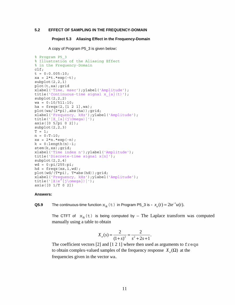
5.2 EFFECT OF SAMPLING IN THE FREQUENCY-DOMAIN

Project 5.3 Aliasing Effect in the Frequency-Domain

A copy of Program P5_3 is given below: % Program P5_3 % Illustration of the Aliasing Effect % in the Frequency-Domain clf; t = 0:0.005:10; xa = 2*t.*exp(-t); subplot(2,2,1) plot(t,xa);grid xlabel('Time, msec');ylabel('Amplitude'); title('Continuous-time signal x_{a}(t)'); subplot(2,2,2) wa = 0:10/511:10; ha = freqs(2,[1 2 1],wa); plot(wa/(2*pi),abs(ha));grid; xlabel('Frequency, kHz');ylabel('Amplitude'); title('|X_{a}(j\Omega)|'); axis([0 5/pi 0 2]); subplot(2,2,3) T = 1; n = 0:T:10; xs = 2*n.*exp(-n); k = 0:length(n)-1; stem(k,xs);grid; xlabel('Time index n');ylabel('Amplitude'); title('Discrete-time signal x[n]'); subplot(2,2,4) wd = 0:pi/255:pi; hd = freqz(xs,1,wd); plot(wd/(T*pi), T*abs(hd));grid; xlabel('Frequency, kHz');ylabel('Amplitude'); title('|X(e^{j\omega})|'); axis([0 1/T 0 2])

Answers:

Q5.9 The continuous-time function xa(t) in Program P5_3 is - ( ) 2 ( ).tax t te u t−=

The CTFT of xa(t) is being computed by – The Laplace transform was computed manually using a table to obtain

2 2

2 2( ) .

(1 ) 2 1aX ss s s

= =+ + +

The coefficient vectors [2] and [1 2 1] where then used as arguments to freqs to obtain complex-valued samples of the frequency response ( )aX Ω at the

frequencies given in the vector wa.

12

Q5.10 The plots generated by running Program P5_3 are shown below:

0 5 100

0.2

0.4

0.6

0.8

Time, msec

Am

plitu

de

Continuous-time signal xa(t)

0 0.5 1 1.50

0.5

1

1.5

2

Frequency, kHz

Am

plitu

de

|Xa(jΩ)|

0 5 100

0.2

0.4

0.6

0.8

Time index n

Am

plitu

de

Discrete-time signal x[n]

0 0.5 10

0.5

1

1.5

2

Frequency, kHz

Am

plitu

de

|X(ejω)|

Based on these results we make the following observations – The analog signal is not bandlimited so there is aliasing. This is particularly visible in the raised tail of | ( ) |jX e ω at 1 kHz relative to the tail of | ( ) |aX Ω .

Q5.11 The plots generated by running Program P5_3 with sampling period increased to 1.5 are shown below:

13

0 5 100

0.2

0.4

0.6

0.8

Time, msec

Am

plitu

de

Continuous-time signal xa(t)

0 0.5 1 1.50

0.5

1

1.5

2

Frequency, kHz

Am

plitu

de

|Xa(jΩ)|

0 2 4 60

0.2

0.4

0.6

0.8

Time index n

Am

plitu

de

Discrete-time signal x[n]

0 0.2 0.4 0.60

0.5

1

1.5

2

Frequency, kHzA

mpl

itude

|X(ejω)|

Based on these results we make the following observations – with the reduction in sampling frequency, the aliasing is now much more severe. The tail of | ( ) |jX e ω is now raised even higher than it was before.

Q5.12 The modified Program P5_3 for the case of xa(t)= e–πt2 is given below: Note:

the CTFT was determined as follows. By applying the time scaling property to

the Fourier transform pair 1 12 22 22t

e eΩ− −←⎯→ π with a scale factor 2 ,a = π we

obtain

2

4( ) .aX eΩ−

πΩ =

Since this function is real and non-negative, we have moreover that ( ) ( ).a aX XΩ = Ω Thus, it is straightforward to include a code in the program

to calculate the CTFT spectrum directly. % Program Q5_12 % Illustration of the Aliasing Effect % in the Frequency-Domain clf; t = 0:0.005:10; xa = exp(-pi*(t.^2)); subplot(2,2,1) plot(t,xa);grid xlabel('Time, msec');ylabel('Amplitude'); title('Continuous-time signal x_{a}(t)'); subplot(2,2,2)

14

wa = 0:10/511:10; ha = exp(-(wa.^2)/(4*pi)); plot(wa/(2*pi),abs(ha));grid; xlabel('Frequency, kHz');ylabel('Amplitude'); title('|X_{a}(j\Omega)|'); axis([0 5/pi 0 1.5]); subplot(2,2,3) T = 1; n = 0:T:10; xs = exp(-pi*(n.^2)); k = 0:length(n)-1; stem(k,xs);grid; xlabel('Time index n');ylabel('Amplitude'); title('Discrete-time signal x[n]'); subplot(2,2,4) wd = 0:pi/255:pi; hd = freqz(xs,1,wd); plot(wd/(T*pi), T*abs(hd));grid; xlabel('Frequency, kHz');ylabel('Amplitude'); title('|X(e^{j\omega})|'); axis([0 1/T 0 1.5])

The plots generated by running the modified Program P5_3 are shown below:

0 5 100

0.5

1

Time, msec

Am

plitu

de

Continuous-time signal xa(t)

0 0.5 1 1.50

0.5

1

1.5

Frequency, kHz

Am

plitu

de

|Xa(jΩ)|

0 5 100

0.5

1

Time index n

Am

plitu

de

Discrete-time signal x[n]

0 0.5 10

0.5

1

1.5

Frequency, kHz

Am

plitu

de

|X(ejω)|

Based on these results we make the following observations – The continuous-time signal ( )ax t is a rapidly decaying Gaussian in this case. Its Fourier transform is therefore a

slowly decaying Gaussian in frequency. As a result, there is even more aliasing in the discrete spectrum this time than in our previous examples. This is not unexpected in

15

view of the fact that we have really only two samples of [ ]x n falling on the main lobe

of ( )ax t .

The plots generated by running the modified Program P5_3 with sampling period increased to 1.5 are shown below:

0 5 100

0.5

1

Time, msec

Am

plitu

deContinuous-time signal x

a(t)

0 0.5 1 1.50

0.5

1

1.5

Frequency, kHz

Am

plitu

de

|Xa(jΩ)|

0 2 4 60

0.5

1

Time index n

Am

plitu

de

Discrete-time signal x[n]

0 0.2 0.4 0.60

0.5

1

1.5

Frequency, kHz

Am

plitu

de

|X(ejω)|

Based on these results we make the following observations – with the sampling rate significantly decreased in this case, the aliasing is now severe. The sampled waveform

[ ]x n has the appearance of a Kronecker delta (discrete-time unit impulse). As a result,

the magnitude spectrum | ( ) |jX e ω is practically flat.

5.3 DESIGN OF ANALOG LOWPASS FILTERS

Project 5.4 Design of Analog Lowpass Filters

A copy of Program P5_4 is given below: % Program P5_4 % Design of Analog Lowpass Filter clf; Fp = 3500;Fs = 4500; Wp = 2*pi*Fp; Ws = 2*pi*Fs; [N, Wn] = buttord(Wp, Ws, 0.5, 30,'s'); [b,a] = butter(N, Wn, 's'); wa = 0:(3*Ws)/511:3*Ws; h = freqs(b,a,wa);

16

plot(wa/(2*pi), 20*log10(abs(h)));grid xlabel('Frequency, Hz');ylabel('Gain, dB'); title('Gain response'); axis([0 3*Fs -60 5]);

Answers:

Q5.13 The passband ripple Rp in dB is – 0.5 dB

The minimum stopband attenuation Rs in dB is - 30 dB

The passband edge frequency in Hz is – 3.5 kHz

The stopband edge frequency in Hz is – 4.5 kHz

Q5.14 The gain response obtained by running Program P5_4 is shown below:

0 2000 4000 6000 8000 10000 12000-60

-50

-40

-30

-20

-10

0

Frequency, Hz

Gai

n, d

B

Gain response

Based on this plot we conclude that the filter designed _MEETS__ the given specifications.

The filter order N is - 18

The 3-dB cutoff frequency in Hz of the filter is – Wn = 3.7144 kHz

17

Q5.15 The required modifications to Program P5_4 to design a Type 1 Chebyshev lowpass filter meeting the same specifications are given below:

% Program Q5_15 % Design of Analog Lowpass Filter clf; Fp = 3500;Fs = 4500; Wp = 2*pi*Fp; Ws = 2*pi*Fs; [N, Wn] = cheb1ord(Wp, Ws, 0.5, 30,'s'); [b,a] = cheby1(N, 0.5, Wn, 's'); wa = 0:(3*Ws)/511:3*Ws; h = freqs(b,a,wa); plot(wa/(2*pi), 20*log10(abs(h)));grid xlabel('Frequency, Hz');ylabel('Gain, dB'); title('Gain response'); axis([0 3*Fs -60 5]); N

The gain response obtained by running the modified Program P5_4 is shown below:

0 2000 4000 6000 8000 10000 12000-60

-50

-40

-30

-20

-10

0

Frequency, Hz

Gai

n, d

B

Gain response

Based on this plot we conclude that the filter designed MEETS_ the given specifications.

The filter order N is - 8

18

The passband edge frequency in Hz of the filter is – Wn = 3.5 kHz

Q5.16 The required modifications to Program P5_4 to design a Type 2 Chebyshev lowpass filter meeting the same specifications are given below:

% Program Q5_16 % Design of Analog Lowpass Filter clf; Fp = 3500;Fs = 4500; Wp = 2*pi*Fp; Ws = 2*pi*Fs; [N, Wn] = cheb2ord(Wp, Ws, 0.5, 30,'s'); [b,a] = cheby2(N, 30, Wn, 's'); wa = 0:(3*Ws)/511:3*Ws; h = freqs(b,a,wa); plot(wa/(2*pi), 20*log10(abs(h)));grid xlabel('Frequency, Hz');ylabel('Gain, dB'); title('Gain response'); axis([0 3*Fs -60 5]); N Wn

The gain response obtained by running the modified Program P5_4 is shown below:

0 2000 4000 6000 8000 10000 12000-60

-50

-40

-30

-20

-10

0

Frequency, Hz

Gai

n, d

B

Gain response

Based on this plot we conclude that the filter designed MEETS_ the given specifications.

The filter order N is -8

19

The stopband edge frequency in Hz of the filter is – 4.2653 kHz

Q5.17 The required modifications to Program P5_4 to design an elliptic lowpass filter meeting the same specifications are given below:

% Program Q5_17 % Design of Analog Lowpass Filter clf; Fp = 3500;Fs = 4500; Wp = 2*pi*Fp; Ws = 2*pi*Fs; [N, Wn] = ellipord(Wp, Ws, 0.5, 30,'s'); [b,a] = ellip(N, 0.5, 30, Wn, 's'); wa = 0:(3*Ws)/511:3*Ws; h = freqs(b,a,wa); plot(wa/(2*pi), 20*log10(abs(h)));grid xlabel('Frequency, Hz');ylabel('Gain, dB'); title('Gain response'); axis([0 3*Fs -60 5]); N Wn/(2*pi)

The gain response obtained by running the modified Program P5_4 is shown below:

0 2000 4000 6000 8000 10000 12000-60

-50

-40

-30

-20

-10

0

Frequency, Hz

Gai

n, d

B

Gain response

Based on this plot we conclude that the filter designed MEETS_ the given specifications.

The filter order N is - 5

20

The passband edge frequency in Hz of the filter is – Wn = 3.5 kHz

5.4 A/D AND D/A CONVERSIONS

Project 5.5 Binary Equivalent of a Decimal Number

Answers:

Q5.18 The function of the operator == is – “==” is a relational operator that returns a value of one if its two operands are equal and a value of zero if its two operands are unequal.

Q5.19 The binary equivalents in sign-magnitude form of the decimal fractions are:

(a) 0 1 1 0 0 1 1; 0 1 1 0 0 1 1 0 1

(b) 1 1 1 0 0 1 1; 1 1 1 0 0 1 1 0 1

(c) 0 1 0 1 0 0 1; 0 1 0 1 0 0 1 0 0

(d) 1 1 1 1 0 1 0; 1 1 1 1 0 1 0 0 1

Project 5.6 Decimal Equivalent of a Binary Number

Answer:

Q5.20 The decimal equivalents of the binary fractions along with the errors in conversion are as follows (Note: use program P5_6fix.m for this. The original program P5_6.m contains errors):

(a) 0.796875 (error=0. 004775); 0.80078125 (error=0.00086875)

(b) -0.796875 (error=-0.004775); -0.80078125 (error=-0.00086875)

(c) 0.640625 (error=0.002705); 0.64062500 (error=0.002705)

(d) -0.90625 (error=-0.00625); -0.91015625 (error=-0.00234375)

Project 5.7 Binary Number Representation Schemes

Answers:

Q5.21 The function of the operator ~ is - (Note: the “~=” operator does not appear in P5_7.m. As stated in the lab manual, what is meant in this question is the “~” operator). The “~” operator performs a bitwise logical complement. Colloquially, it “flips the bits.” It turns each “zero bit” into a “one bit” and each “one bit” into a “zero bit.”

Q5.22 The ones'-complement representations of the binary numbers developed in Question Q5.19 are as follows:

21

(a) 0 1 1 0 0 1 1; 0 1 1 0 0 1 1 0 1

(b) 1 0 0 1 1 0 0; 1 0 0 1 1 0 0 1 0

(c) 0 1 0 1 0 0 1; 0 1 0 1 0 0 1 0 0

(d) 1 0 0 0 1 0 1; 1 0 0 0 1 0 1 1 0

Q5.23 The function of the operator | is – The “|” operator performs a bitwise logical OR operation on its operands.

The function of the operator & is – The “&” operator performs a bitwise logical AND operation on its operands.

Q5.24 The two's-complement representations of the binary numbers developed in Question Q5.19 are as follows: Note: It’s important to realize that P5_8 works differently from the others. For non-negative fractions, the representation in two’s complement, one’s complement, and signed magnitude are all exactly the same. The only difference is in the representation of negative fractions. P5_8 only works for negative fractions. For input, it takes the one’s complement representation of the negative fraction. For output, it produces the two’s complement representation of that same negative fraction. In particular, this means that the answers to Q5.24 (a) and (c) are the same as the answers to Q5.22 (a) and (c) and Q5.19 (a) and (c).

(a) 0 1 1 0 0 1 1; 0 1 1 0 0 1 1 0 1

(b) 1 0 0 1 1 0 1; 1 0 0 1 1 0 0 1 1

(c) 0 1 0 1 0 0 1; 0 1 0 1 0 0 1 0 0

(d) 1 0 0 0 1 1 0; 1 0 0 0 1 0 1 1 1

Project 5.8 D/A Converter Droop Compensation

Answer:

Q5.25 The MATLAB program to determine and plot the magnitude responses of the uncompensated and the droop-compensated D/A converters is given below:

Notes on the Program Development: The sampling interval is ,T which will be set to 1T = by default in the program. The uncompensated DAC is modeled as a series connection of two continuous-time systems: the ideal reconstruction filter ( )rH jΩ given in (5.10) on page 72 of

the lab manual and the zero-order hold model ( )zH jΩ given in (5.27) on page 78 of the lab

manual. All frequency response magnitudes will be plotted against a vector of 512 frequency samples equally spaced between DC and / 2 /s TΩ = π rad/sec. To plot the gain of the

uncompensated DAC, we simply evaluate ( ) ( )r zH j H jΩ Ω and convert to dB. To evaluate

( )zH jΩ at the point 0,Ω = it is necessary to apply L’Hopital’s rule as follows:

22

lim lim

20 0 0

0 lim lim0 0

sin( / 2) cos( / 2)lim ( ) 1 1.

( / 2) ( / 2)

T

z

T TH j e

T T

∂∂ΩΩ→ Ω→

∂Ω→∂ΩΩ→ Ω→

Ω ΩΩ = × = × =

Ω

For the other frequency samples, ( )zH jΩ can be evaluated directly using formula (5.27)

of the lab manual.

For the two systems with digital droop compensation, we consider that the series connection of the digital compensation filter with the ideal reconstruction filter results in an equivalent analog compensation filter that is in series with ( )zH jΩ and ( )rH jΩ . For the FIR compensation filter,

we have from (5.29) on page 86 of the lab manual that

( )1 1 216

( ) 1 18FIRH z z z− −= − + − ,

from which we obtain

( )1 216

( ) 1 18 .j j jFIRH e e eω − ω − ω= − + −

The frequency response of the equivalent analog compensation filter that is realized by the series combination of ( )FIRH z with the ideal DAC ( )rH jΩ is given by

( )

( )

,

1 216

, /( )

0 /

1 18 , /.

0 /

j TFIR

FIR a

j T j T

H e TH j

T

e e T

T

Ω

− Ω − Ω

Ω ≤ πΩ = Ω > π

− + − Ω ≤ π= Ω > π

The overall magnitude response of the FIR compensated DAC is then given by

,( ) ( ) ( ) ,r FIR a zH j H j H jΩ Ω Ω which will be evaluated by the program and converted to

units of dB for plotting. For the IIR compensation filter, we have from (5.30) on page 86 of the lab manual that

( ) 9,

8j

IIR jH e

eω

− ω=+

so

( ),

, /( )

0 /

9, /

.80 /

j TIIR

IIR a

j T

H e TH j

T

Te

T

Ω

− Ω

Ω ≤ πΩ = Ω > π

Ω ≤ π= + Ω > π

The overall magnitude response of the IIR compensated DAC is then given by

,( ) ( ) ( ) ,r IIR a zH j H j H jΩ Ω Ω which will be evaluated by the program and converted to

units of dB for plotting.

23

The program is given below. % Program Q5_25.m % For a non-ideal sample-and-hold D/A converter, % compute the magnitude response of % 1. the uncompensated D/A % 2. D/A with FIR droop compensation % 3. D/A with IIR droop compensation % all on a single graph. T = 1.0; % sampling interval wa = 0:(pi/T)/511:(pi/T); % analog freq vector Lwa = length(wa); Hra = T * ones(1,length(wa)); % ideal reconstruction filter % Frequency response of uncompensated zero-order hold Hza = zeros(1,Lwa); Hza(1) = 1; % follows from L'Hopital's Rule wa2 = wa(2:Lwa); Hza(2:Lwa) = exp(-i*wa2*T*0.5) .* sin(0.5*T*wa2) ./ (0.5*T*wa2); MagHza = abs(Hza); GainHza = 20*log10(MagHza); % Frequency response of FIR compensated D/A Hfira = (1/16)*(-1 + 18*exp(-i*wa*T) - exp(-i*2*T*wa)); HfiraComp = Hfira .* Hza; MagHfiraComp = abs(HfiraComp); GainHfiraComp = 20*log10(MagHfiraComp); % Frequency response of IIR compensated D/A Hiira = 9*ones(1,Lwa) ./ (8 + exp(-i*wa*T)); HiiraComp = Hiira .* Hza; MagHiiraComp = abs(HiiraComp); GainHiiraComp = 20*log10(MagHiiraComp); % plot plot(wa,GainHza,wa,GainHfiraComp,'--',wa,GainHiiraComp,'-.'); grid; xlabel('Frequency'); ylabel('Gain, dB'); axis([0 pi/T -4 1]); legend('DAC','FIR','IIR');

24

The plot of the magnitude responses is shown below:

0 0.5 1 1.5 2 2.5 3-4

-3.5

-3

-2.5

-2

-1.5

-1

-0.5

0

0.5

1

Frequency

Gai

n, d

B

DAC

FIRIIR

From this plot we make the following observations: Both the FIR and IIR compensated DACS offer a significant improvement in terms of reducing the droop of the uncompensated DAC. The spectral magnitude of the IIR compensated DAC is slightly flatter in the pass band and rolls off slightly slower than the FIR compensated DAC. It is interesting to note that this plot is in perfect agreement with the one given in Fig. 4.56 on page 224 of the course text.

Date: 21 October 2009 Signature: SOLUTION (Havlicek)