ELECTROLYTE SOLUTIONS

Electrolyte solutions historically set themselves apart from ordinary solutions in the study of mixtures.For many years, standard texts on solutions were written fornonelectrolytes(e.g., Hildebrand and Scott[1]). This fact bespeaks the difficulty in treating electrically charged species. One of the earliest efforts indescribing dissolved salts was undertaken by Debye and H¨uckel [2]. However, it was not until the 1960sand 1970s when liquid state theories had well developed that a common approach to electrolyte and non-electrolyte solutions became possible. The common basis is the molecular distribution functions. (For ahistorical review, see FalkenhagenElectrolytes [3]). In this chapter, we present one of the statisticalmechanical models for electrolyte solutions, namely thecharged hard spheres. This model, though simple,represents an important advance in the study of concentrated electrolyte solutions.

Statistical mechanics treats the ionized species in the same way as it treats ordinary fluids, i.e., byconsidering the Hamiltonian of an N-body system consisting of cations, anions, and solvent molecules.The power of the statistical methods lies in their ability of treating particles of dissimilar nature on the samebasis. The electrostatic Coulomb forces developed for macroscopic bodies are assumed to operate on themolecular level. Statistical mechanics is used to provide the laws governing the distribution of particles.For example, the Boltzmann distribution used in the Debye-H¨uckel (DH) theory is a special case of statisti-cal distributions. As we shall see, this distribution is uniquely determined by the Hamiltonian of the sys-tem.

Debye and H¨uckel introduced a model for electrolyte solutions where the ions are treated aspointelectric charges(i.e., charges havingno excluded volume) obeying classical electrostatic principles (thePoisson equation). The charge density is given by an exponential distribution law (Boltzmann distribution).It is successful in describing dilute solution properties. As such, the DH theory was considered a milestonein electrolyte theories. However, for concentrated solutions, the point charge model is no longer valid.Large deviations in osmotic and mean activity coefficients are observed. Thus DH is not quantitative athigh ionic strengths. Obviously, new and more accurate theories need be developed.

In the intervening years, progress was made due to efforts by Mayer [4], Bjerrum [5], Guggenheim[6], and others. In the 1970s, an integral equation theory, the mean spherical model (MSA), was solved forcharged hard spheres with finite size. This success represents another step forward in modeling ionic solu-tions, because it takes the sizes of ions into account. The solution given by MSA reveals an intricate inter-play between ion size and charge strength. Further developments along the liquid distribution functionapproach produced the Percus-Yevick (PY) and hypernetted chain (HNC) version for electrolyte solutions.Meanwhile, Monte Carlo (MC) simulations were performed for the so-called primitive model of ionic solu-tions (see below). These developments are instrumental in the establishment of a quantitative theory.

In this chapter, we study a model electrolyte, i.e., mixtures of charged hard spheres of finite sizes.The solvent molecules, on the other hand, are not explicitly treated. For example, the water molecules areremoved and replaced by a dielectric continuum. This idealization of the ionic solutions is called theprimi-tive model.For aqueous solutions, the dielectric medium will have the permittivity of water. As a conse-quence, the electrostatic forces of interaction, which are Coulombic in nature, retain their values in water.Such treatment of solvents was earlier considered by McMillan and Mayer [7] and is called the McMillan-Mayer theory of solutions.

We note a number of limitations of the primitive model. The water molecules, being of similardimension as the ions, are actuallygranular, i.e., visible to the charged ions through hydration or simpleexclusion. Recent studies have examined the effects of thegranularity by injecting dipolar spheres (simu-lating water molecules) into the primitive model. However, a full-scale treatment of water molecules interms of more sophisticated potential models (such as the Matsuoka-Clementi-Yoshimine potential[8]) is at

present a formidable task. There are major theoretical difficulties in treating aqueous ionic solutions. Sec-ond, the repulsive interactions among ions are not so harsh as suggested by the hard sphere model. Keep-ing these points in mind, we should consider the primitive model as an approximation for real electrolytesolutions. Attempts have been made to apply the PM model to describe real salt solutions. Due to theselimitations, it has been found that an adjustable ionic diameter or a state-dependent dielectric constant hasto be used in order to achieve quantitative agreement.

In the l970s, Waisman and Lebowitz [9] solved the MSA for the restricted primitive model. A rapidsuccession of new results on more sophisticated models of ionic solutions ensued. The MSA equationshave been solved for asymmetrical ions, mixtures of charged hard spheres and dipolar spheres, and chargedparticles near a wall. The MSA itself has been improved in many ways by the techniques of cluster resum-mations (e.g. in the optimized random phase approximation (ORPA) [9] and theΓ-ordering theory [10]).Other integral equations have been tested and shown promise, such as the PY-type equation (e.g., Allnatt[11]) and the HNC [12]. Due to progress in numerical transform techniques (e.g., the fast Fourier trans-form), the HNC equation has recently been applied to charged soft spheres. Computer simulations on theCoulombic andscreenedCoulombic systems were also carried out. New features of the structure of ionicsolutions have been discovered. All these developments add considerably to our understanding of elec-trolyte solutions.

Since the DH theory has played a major role at the early stages of solution theories, we devote sec-tions XII.3 and 4 to a full account. The DH theory is limited to dilute solutions where only long-rangeelectrostatic forces are at work and short-range interactions are absent. For concentrated solutions, theshort-range electrostatic and exclusion forces become more important. Thus the primitive model postulatesa finite impenetrable core for the ions. The MSA results for this model are presented in section XII.5. Incomparison with simulation data, the energy values predicted by MSA are accurate but the structure givenby MSA is rather poor. In section XII.6, asymmetrical ions are considered. It is found that the HNC equa-tion is by far the most accurate theory for ionic potentials. Section XII.7 is devoted to a study of HNC. Wealso show results for solvent effects using the LHNC and QHNC equations. The moment conditions due toStillinger and Lovett are discussed. In addition, we give an account of the simulation results for Coulomband screened Coulomb potentials.

XII.1. Review of Electrostatics

In order to discuss the forces and potentials for charged molecules, we need to review the funda-mental laws in classical electrostatics. An important point to keep in mind is that for classical systems thelaws governing macroscopic bodies also apply to molecules. First we discuss Coulomb’s law.

COULOMB’S LAW

Coulomb’s law simply states that for two point chargesq1 and q2 separated by a distancer , theforceF exerted along the line joining the two charges is given by

(1.1)F12 =1

ε m

q1q2

r 2u12

whereε m is the permittivity of the medium where the two charges are embedded,u12 is the unit vector inthe direction ofr12 = r2 − r1, andr = |r12|. Note that here we have adopted the convention omitting the fac-tor 4π from the denominator in the definition of the permittivity (4π accounts for the solid angle in sphericalgeometry). For free space (i.e., vacuum),ε0 = 111.2× 10−12 Coulomb2/N m2 or (ε0)−1 = 9 ×109

N − m2/Coulomb2. In a medium with permittivityε m the dielectric constantε is defined as the ratio

(1.2)ε ≡ε m

ε0

For vacuum, the dielectric constant is 1. In literature, the nomenclature forε andε m is not always distinct.The statement thatε is a dielectric constantmay mean either the permittivityε m or the dielectric constantε(a ratio). One must decide from the context ifε stands for permittivity or otherwise. Here, we adhere todistinct notations.

GAUSS’S LAW

Gauss’s law deals with the electric field on the surface of a body enclosing a distribution of charges.It is expressed in terms of an integral

(1.3)C∫

S∫ E ⋅ dS =

k

i=1Σ 4π qi

ε m

whereE is the electric field given by

(1.4)E1 =F12

q1

whereF12 is the force given by Coulomb’s law (1.1); i.e.,E1 is the electric force per unit charge at locationr1. In eq. (1.3), the integration is over a closed (regular) surface (CS) enclosing a volume that containskseparate centers of chargesqi (i=1,...,k). The integrand is the dot (inner) product of the electric fieldE withsurface elementdS whose magnitude is the surface area and whose direction is that of the outward pointednormaln. Simply stated, (1.3) states that the projection of the mean electric field on the surface is equal tothe sum of the charges inside the body (divided by the permittivityε m of the medium). When the chargedistribution inside the body is continuous, the sum of charges should be replaced by an integral; i.e.,

(1.5)C∫

S∫ E ⋅ dS =

4πε m

∫Vb

∫ ∫ ρe dV

whereρe is the electrical charge density (charges per volume), andVb is the volume of the body. We hav estated these theorems without proof. One should consult texts [13] on electromagnetism for details.

POISSON’S EQUATION

The Poisson equation can be easily derived from Gauss’s law. In mathematics, Green’s div ergencetheorem states

(1.6)C∫

S∫ dS∇φ ⋅ n = ∫

Vb

∫ ∫ dV ∇ ⋅ ∇φ

where CS encloses the volumeVb. ∇ is the gradient operator, andφ is some scalar potential. Equation (1.6)says that the accumulation of the normal component of the gradient ofφ on the surface is equal to the vol-ume integral of the Laplacian ofφ. Now if the electric fieldE is expressed as the gradient of some potentialfunctionφ, i.e.,E = − ∇φ , we hav e immediately from (1.5)

(1.7)− ∫Vb

∫ ∫ dV ∇ ⋅ ∇φ =4πε m

∫Vb

∫ ∫ dV ρe

Since the volumeVb is arbitrary, the integrands on both sides of (1.7) must be equal:

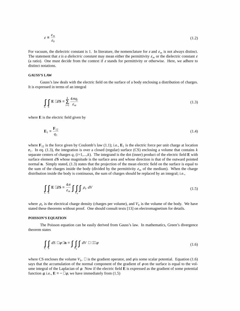
(1.8)∆φ = −4πε m

ρe

where the Laplacian∆ = ∇ ⋅ ∇. This is Poisson’s equation.

XII.2. The McMillan-Mayer Theory of Solutions

A number of solution theories in use make the simplifying assumption that the solvent moleculesaresmearedout, forming a uniform background, called thedielectricor neutralizing continuum(e.g., in theprimitive model of electrolyte solutions or in the one-component plasmas, respectively). Thissmoothingoperation has the advantage of reducing considerably the level of difficulty since the solvent molecules, thehydrogen-bonding water, no longer figure explicitly in the formulation. What remains of the water is itspermittivity, becauseε m of the medium is set equal to that of water. Such a viewpoint is employed in theMcMillan-Mayer (MM) theory of solutions. The important task is to find a way ofaveragingout the sol-vent molecules while preserving their effects.

We start by considering an experiment of osmosis: a pure solventw (e.g., water) is placed in parti-tion I of a container and separated by a semipermeable membrane from partition II containing a solutionwith solutea and solventw. The membrane allows passage of water molecules but not solute molecules.At equilibrium, the system is isothermal, and the activity of water,zI

w in I must be equal tozIIw in II. How-

ev er, in partition II,zIIw would be less than its pure component counterpart, given the same pressure and

temperature, becausew is mixed witha in partition II. To increase its activity to the level in I, we mustincrease the system pressure on II,PII , abovePI . When equalityzI

w = zIIw has eventually established, we

find PII > PI . The differencePosm = PII − PI is called theosmotic pressure. As in the case of fluids,Posm

is a function of the concentration of the solute as well as the temperature and the pressure of the system.Next, we present the MM theory of solutions. Since we are dealing with an open system, we shall

use the grand canonical ensemble (GCE). In order to distinguish between the exact and MM approaches,we use one asterisk (*) to denote the exact ensemble quantities and two asterisks (**) to denote the aver-aged quantities where the solvent (e.g., water) molecules have beensmoothedout. The av eraging is appliedto partition II.

In the GCE the partition functionΞ is related to the thermodynamic pressure by

(2.1)Ξ * I = exp(β I PIV I ) (region I)

(2.2)Ξ * II = exp(β II PIIV II ) (region II)

where the superscripts I and II denote the properties in regions I and II, respectively. The MM partitionfunction for region II is defined as

(2.3)Ξ * * II ≡Ξ * II

Ξ * I= exp(β PosmV)

wherePosm = PII − PI . We hav e setV I = V II . Also β I = β II at equilibrium.

Next we want to find the expression forΞ** in terms of an exact description. First we rewrite thedefinitions ofΞ* and theN+M-tuplet correlation function as

(2.4)Ξ * =∞

N≥0Σ

∞

M≥0Σ zN

a zMw

N!M !Q*

N+M

and

(2.5)g * (n+m) (1a, 2a, . . . ,na; 1w, 2w, . . . ,mw; za, zw)

= ρ−na ρ−m

w Ξ *−1∞

N≥nΣ

∞

M≥mΣ zN

a zMw

(N − n)!(M − m)!

⋅ ∫ d(n + 1)a . . .dNad(m + 1)w . . .dMw e−βVN+M

where

(2.6)Q*N+M = ∫ d1a d2a

. . .dNa d1w d2w. . .dMw exp(−βVN+M )

andVN+M is the total potential energy ofN solute molecules andM solvent molecules. The above defini-tions are for a mixture of one solute speciesa and one solvent speciesw. For multicomponent mixtures,the expressions can be generalized. In order to examine the details, we write out the series forΞ*:

(2.7)Ξ * I = 1 +zw

1!Q*

0+1 +z2

w

2!Q*

0+2 +z3

w

3!Q*

0+3 + . . .

and

(2.8)Ξ * II = 1 +za

1!0!Q*

1+0 +zw

0!1!Q*

0+1 +zazw

1!1!Q*

1+1 +z2

a

2!0!Q*

2+0 +z2

w

0!2!Q*

0+2 + . . .

= 1 +

zw

1!Q*

0+1 +z2

w

2!Q*

0+2 + . . .

+za

1!Q*

1+0 +zw

1!Q*

1+1 +z2

w

2!Q*

1+2 + . . .

+z2

a

2!Q*

2+1 +zw

1!Q*

1+1 +z2

w

2!Q*

2+2 + . . .

+ . . .

The first pair of parentheses of (2.8) is simplyΞ * I . Thus division ofΞ * II by Ξ * I gives

(2.9)Ξ * II

Ξ * I= 1 + (Ξ* I)−1 za

1!

∞

M≥0Σ zM

w

M !Q*

1+M

+(Ξ* I)−1 z2a

2!

∞

M≥0Σ zM

w

M !Q*

2+M

+ . . .

Thus the MM partition function has the form

(2.10)Ξ * * II =∞

N≥0Σ zN

a

N!kN

a Q**N = 1 +

za

1!kaQ**

1 +z2

a

2!k2

aQ**2 + . . .

whereka and Q**1 ,Q**

2 ,..., etc., are quantities to be determined by comparison with the exact expression(2.9). If we equate coefficients of same powers in activityza, we hav e

(2.11)kNa Q**

N =1

Ξ * I

∞

M=0Σ zM

w

M !Q*

N+M

There is some arbitrariness in assigning values toka andQ**N . The choice made by Friedman et al. [14] is

to consider first the related quantity

(2.12)∫ d1a d2a. . .dNa g * (N+0) (1a, 2a, . . . ,Na; za, zw)

=1

ρ Na

1

Ξ * II

zN

a Q*(N+0) +

zN+1a

1!0!Q*

(N+1)+0 +zN+1

a zw

1!1!Q*

(N+1)+1 +zN

a zw

0!1!Q*

N+1 + . . .

This is not quite the quantity yet we wanted in (2.11). We note that in the limitza → 0, za/ρ a = 1, and

(2.13)za→0lim Ξ * II = Ξ * I

Thus

(2.14)za→0lim ∫ d1a

. . .dNa g * (N+0) (1a, . . . ,Na; za = 0,zw)

=za→0

lim

zNa

ρ Na

1

Ξ * I

Q*

N+0 +zw

1!Q*

N+1 +z2

w

2!Q*

N+2 + . . .

The term in the braces is precisely the summation in (2.11). Thus we can write

(2.15)kNa Q**

N =za→0lim

ρ Na

zNa

∫ d1a. . .dNa g * (N+0) (1a, . . . ,Na; za = 0,zw)

Friedman et al. (Ibid.) chose

(2.16)ka ≡za−>0lim

ρ a

za

and

(2.17)Q**N ≡

za→0lim ∫ d1a

. . .dNa g * (N+0) (1a,. . . ; Na; za = 0,zw)

If we define the potential of mean forceW * (N+M) by

(2.18)W * (N+0) (1a, . . . ,Na; za, zw) ≡ − kT ln g * (N+0) (1a, . . . ,Na; za, zw)

the MM configurational partition function can be written in the familiar form

(2.19)Q**N =

za→0lim ∫ d1a

. . .dNa exp−βW * (N+0) (1a, . . . ,Na; za, zw)

Finally,

(2.20)Ξ * * II =∞

N≥0Σ z** N

a

N! ∫ d1a. . .dNa exp

−β

za→0lim W * (N+0) (1a, . . . ,Na, za,zw)

with

(2.21)z**a ≡ zaka = za

za→0

limρ a

za

We hav e succeeded in expressing the MM partition function in terms of the potential of mean forceW * (N+0) of the exact ensemble. Since the potential of mean force depends on the solvent activityzw andthe temperature through (2.18) (note that theN-tuplet correlation functiong * (N+0) depends on these vari-ables), the potential energy of the ionic system (after excluding the solvent) is no longer constant and isstate-dependent, a price to pay for simplification. Note that the limitza → 0 denotes infinite dilution quan-tities, i.e., when the solute molecules disappear from the solution.

In the following, we shall incorporate the MM theory in the primitive model of ionic solution. Insection XII.7, we shall discuss the effects of solventgranularity whereby the solvent molecules are treatedexplicitly. As eq. (2.20) retains the form of a partition function, we could derive the thermodynamic prop-erties as usual. Also from the definition ofΞ** (2.3), the pressure we obtain from the MM theory is theosmotic pressure, not the system pressureP.

XII.3 . The Debye-Huckel Theory

The DH theory is of historical significance in electrolyte solutions. It is now recognized as the lim-iting law at infinite dilution. In this theory, the ions are point charges and the solvent molecules arereplaced by a dielectric continuum with the permittivityε H2O of water. For charged hard spheres, the poten-tial between ion 1 and ion 2 is given by the Coulomb interaction subject to hard core repulsion

(3.1)u(r12) = + ∞, r ≤ d

=z1z2e2

ε mr12, r > d

For DH, the diameterd is taken to be zero (no hard core).zj , ( j= 1,2), is the valence of the charged ionj(for example, in sodium sulfate Na2SO4, z+ = + 1 for the cation andz− = − 2 for the anion);e is the chargeof an electron, i.e.,−1.602× 10−19 Coulomb or, in electrostatic units,−4.803× 10−10 esu. We usually takethe absolute value |e| in what follows.

When salts such as NaCl dissolve in water, the ions Na+ and Cl− dissociate and separate from eachother. Howev er, the attractive Coulomb force between oppositely charged ions should recombine Na+ withCl−. What prevents them from coalescing into a neutral molecule? The answer is to be found in the largevalues of the dielectric constant of water, 80.176 at 20°C. The high permittivity accounts for the existence

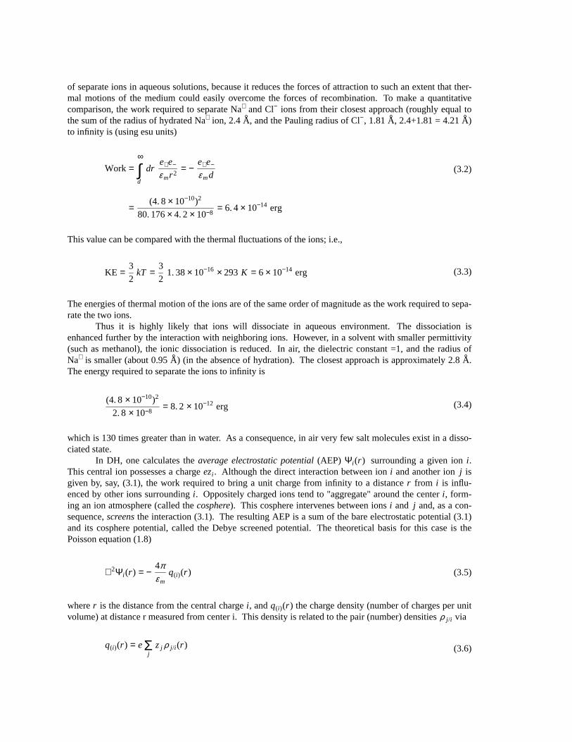
of separate ions in aqueous solutions, because it reduces the forces of attraction to such an extent that ther-mal motions of the medium could easily overcome the forces of recombination. To make a quantitativecomparison, the work required to separate Na+ and Cl− ions from their closest approach (roughly equal tothe sum of the radius of hydrated Na+ ion, 2.4 A° , and the Pauling radius of Cl−, 1.81 A° , 2.4+1.81 = 4.21 A° )to infinity is (using esu units)

(3.2)Work =∞

d∫ dr

e+e−

ε mr 2= −

e+e−

ε md

=(4. 8× 10−10)2

80. 176× 4. 2× 10−8= 6. 4× 10−14 erg

This value can be compared with the thermal fluctuations of the ions; i.e.,

(3.3)KE =3

2kT =

3

21. 38× 10−16 × 293 K = 6 × 10−14 erg

The energies of thermal motion of the ions are of the same order of magnitude as the work required to sepa-rate the two ions.

Thus it is highly likely that ions will dissociate in aqueous environment. The dissociation isenhanced further by the interaction with neighboring ions. However, in a solvent with smaller permittivity(such as methanol), the ionic dissociation is reduced. In air, the dielectric constant =1, and the radius ofNa+ is smaller (about 0.95 A° ) (in the absence of hydration). The closest approach is approximately 2.8 A° .The energy required to separate the ions to infinity is

(3.4)(4. 8× 10−10)2

2. 8× 10−8= 8. 2× 10−12 erg

which is 130 times greater than in water. As a consequence, in air very few salt molecules exist in a disso-ciated state.

In DH, one calculates theaverage electrostatic potential(AEP) Ψi (r ) surrounding a given ioni .This central ion possesses a chargeezi . Although the direct interaction between ioni and another ionj isgiven by, say, (3.1), the work required to bring a unit charge from infinity to a distancer from i is influ-enced by other ions surroundingi . Oppositely charged ions tend to "aggregate" around the centeri , form-ing an ion atmosphere (called thecosphere). This cosphere intervenes between ionsi and j and, as a con-sequence,screensthe interaction (3.1). The resulting AEP is a sum of the bare electrostatic potential (3.1)and its cosphere potential, called the Debye screened potential. The theoretical basis for this case is thePoisson equation (1.8)

(3.5)∇2Ψi (r ) = −4πε m

q(i)(r )

wherer is the distance from the central chargei , andq(i)(r ) the charge density (number of charges per unitvolume) at distance r measured from center i. This density is related to the pair (number) densitiesρ j /i via

(3.6)q(i)(r ) = ej

Σ zj ρ j /i (r )

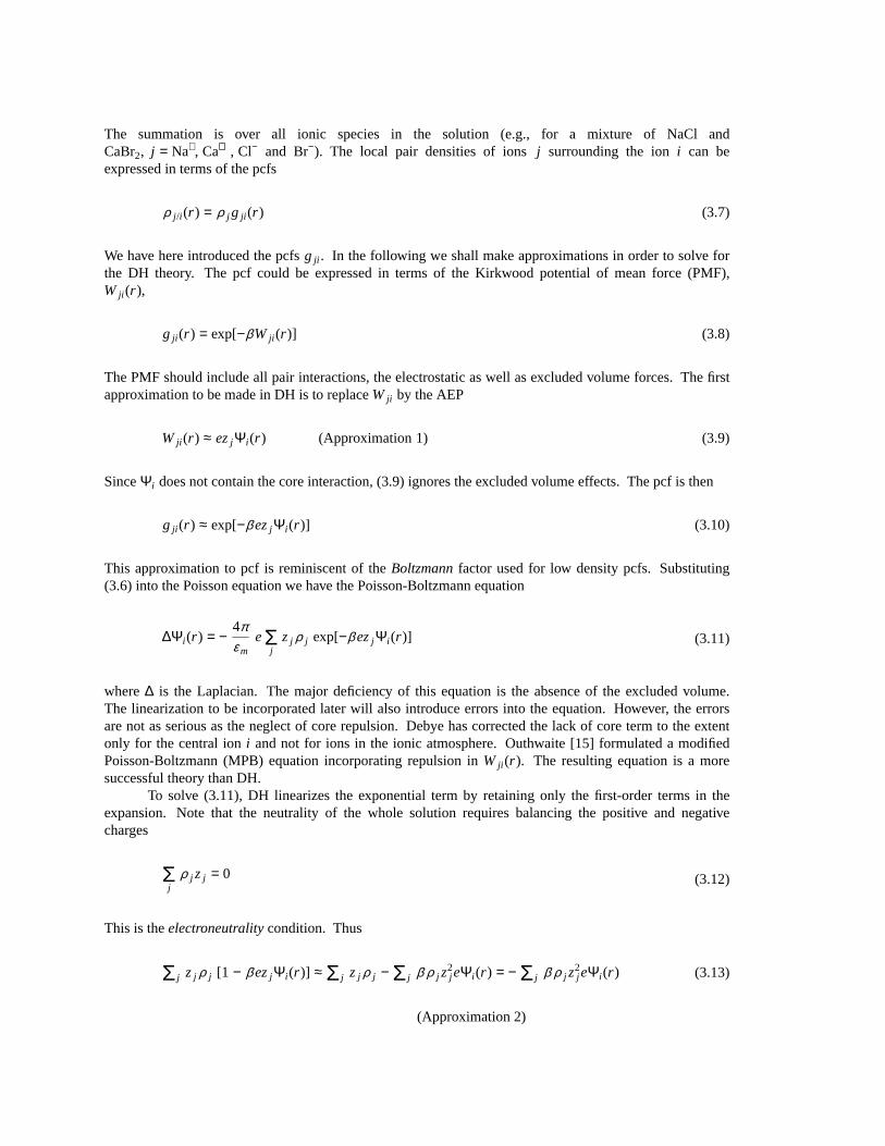
The summation is over all ionic species in the solution (e.g., for a mixture of NaCl andCaBr2, j = Na+, Ca++, Cl− and Br−). The local pair densities of ionsj surrounding the ioni can beexpressed in terms of the pcfs

(3.7)ρ j /i (r ) = ρ j g ji (r )

We hav e here introduced the pcfsgji . In the following we shall make approximations in order to solve forthe DH theory. The pcf could be expressed in terms of the Kirkwood potential of mean force (PMF),Wji (r ),

(3.8)gji (r ) = exp[−βWji (r )]

The PMF should include all pair interactions, the electrostatic as well as excluded volume forces. The firstapproximation to be made in DH is to replaceWji by the AEP

(3.9)Wji (r ) ≈ ezj Ψi (r ) (Approximation 1)

SinceΨi does not contain the core interaction, (3.9) ignores the excluded volume effects. The pcf is then

(3.10)gji (r ) ≈ exp[−β ezj Ψi (r )]

This approximation to pcf is reminiscent of theBoltzmannfactor used for low density pcfs. Substituting(3.6) into the Poisson equation we have the Poisson-Boltzmann equation

(3.11)∆Ψi (r ) = −4πε m

ej

Σ zj ρ j exp[−β ezj Ψi (r )]

where∆ is the Laplacian. The major deficiency of this equation is the absence of the excluded volume.The linearization to be incorporated later will also introduce errors into the equation. However, the errorsare not as serious as the neglect of core repulsion. Debye has corrected the lack of core term to the extentonly for the central ioni and not for ions in the ionic atmosphere. Outhwaite [15] formulated a modifiedPoisson-Boltzmann (MPB) equation incorporating repulsion inWji (r ). The resulting equation is a moresuccessful theory than DH.

To solve (3.11), DH linearizes the exponential term by retaining only the first-order terms in theexpansion. Note that the neutrality of the whole solution requires balancing the positive and negativecharges

(3.12)j

Σ ρ j zj = 0

This is theelectroneutralitycondition. Thus

(3.13)Σ j zj ρ j [1 − β ezj Ψi (r )] ≈ Σ j zj ρ j − Σ j β ρ j z2j eΨi (r ) = − Σ j β ρ j z

2j eΨi (r )

(Approximation 2)

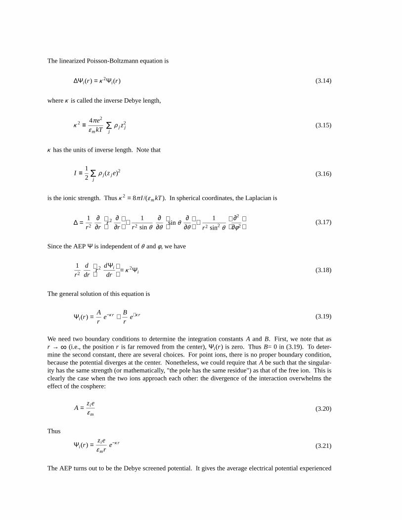
The linearized Poisson-Boltzmann equation is

(3.14)∆Ψi (r ) = κ 2Ψi (r )

whereκ is called the inverse Debye length,

(3.15)κ 2 ≡4π e2

ε mkT jΣ ρ j z

2j

κ has the units of inverse length. Note that

(3.16)I ≡1

2 jΣ ρ j (zj e)2

is the ionic strength. Thusκ 2 = 8π I /(ε mkT). In spherical coordinates, the Laplacian is

(3.17)∆ =1

r 2

∂∂r

r 2 ∂

∂r

+1

r 2 sinθ∂

∂θsinθ

∂∂θ

+1

r 2 sin2 θ

∂2

∂φ2

Since the AEPΨ is independent ofθ andφ , we hav e

(3.18)1

r 2

d

drr 2 dΨi

dr

= κ 2Ψi

The general solution of this equation is

(3.19)Ψi (r ) =A

re−κ r +

B

re+κ r

We need two boundary conditions to determine the integration constantsA and B. First, we note that asr → ∞ (i.e., the positionr is far removed from the center),Ψi (r ) is zero. ThusB= 0 in (3.19). To deter-mine the second constant, there are several choices. For point ions, there is no proper boundary condition,because the potential diverges at the center. Nonetheless, we could require thatA be such that the singular-ity has the same strength (or mathematically, "the pole has the same residue") as that of the free ion. This isclearly the case when the two ions approach each other: the divergence of the interaction overwhelms theeffect of the cosphere:

(3.20)A =zi e

ε m

Thus

(3.21)Ψi (r ) =zi e

ε mre−κ r

The AEP turns out to be the Debye screened potential. It gives the average electrical potential experienced

by a unit charge atr due to interactions with the central ioni and its cosphere. Naturally, for each specieskin the ionic solution, one could write down an equation of the form (3.21). As a consequence, DH theoryimplies that the PMF is of the form

(3.22)Wji (r ) = ezj Ψi (r )

and the pcf

(3.23)gji (r ) = exp[−β ezj Ψi (r )] ≈ 1 −e2zj zi

ε mkT

e−κ r

r

upon linearizing the exponential.We recall that the DH theory contains two approximations: (i) neglect of the excluded volume, and

(ii) linearization of the Boltzmann factor. The physical basis of DH is the classical Poisson equation. How-ev er, it is also possible to derive the screened potential from statistical mechanics, in this case from the Orn-stein-Zernike (OZ) relation for correlation functions. Simplifying assumptions will have to be made. Thisis done next.

XII.4 . Derivation from Statistical Mechanics

Let us consider, for simplicity, a single salt dissolved in water. In the MM picture, the solvent isreplaced by the dielectric background. The OZ relation for the ion species can be written as

(4.1)hij (rr ′) − Cij (rr ′) =lΣ ρ l ∫ ds Cil (rs)hlj (sr′)

In order to reproduce the DH results, we assume low salt concentrations. Thus the limiting law clusterexpansions ofhij andCij could be used; i.e.,

(4.2)Cij = fij = e−β uij − 1 ≈ −uij

kT

(This approximation is similar to MSA.)

(4.3)hij = e−βWij − 1 ≈ −Wij

kT

whereWij is again the potential of mean force. The second equality is valid only at high temperatures. Theinteraction potentialuij is given by (3.1). Thus (4.1) becomes

(4.4)− Wij (r ) = −zi zj e

2

ε mr+

lΣ β ρ l ∫ ds

zi zl e2

ε msWlj (|r − s|)

We assume the solution ofWij to be of the form

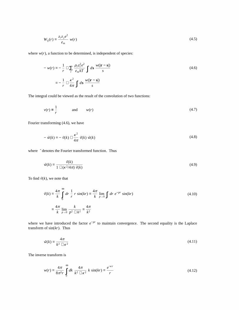
(4.5)Wij (r ) =zi zj e

2

ε mw(r )

wherew(r ), a function to be determined, is independent of species:

(4.6)− w(r ) = −1

r+

lΣ ρ l z

2l e2

ε mkT ∫ dsw(|r − s|)

s

= −1

r+

κ 2

4π ∫ dsw(|r − s|)

s

The integral could be viewed as the result of the convolution of two functions:

(4.7)v(r ) ≡1

rand w(r )

Fourier transforming (4.6), we have

(4.8)− w(k) = − v(k) +κ 2

4πv(k) w(k)

where ˜ denotes the Fourier transformed function. Thus

(4.9)w(k) =v(k)

1 + (κ 2/4π ) v(k)

To find v(k), we note that

(4.10)v(k) =4πk

∞

0∫ dr

1

rr sin(kr) =

4πk p→0

lim ∫ dr e−pr sin(kr)

=4πk p→0

limk

p2 + k2=

4πk2

where we have introduced the factore−pr to maintain convergence. The second equality is the Laplacetransform of sin(kr). Thus

(4.11)w(k) =4π

k2 + κ 2

The inverse transform is

(4.12)w(r ) =4π

8π 3r

∞

0∫ dk

4πk2 + κ 2

k sin(kr) =e−κ r

r

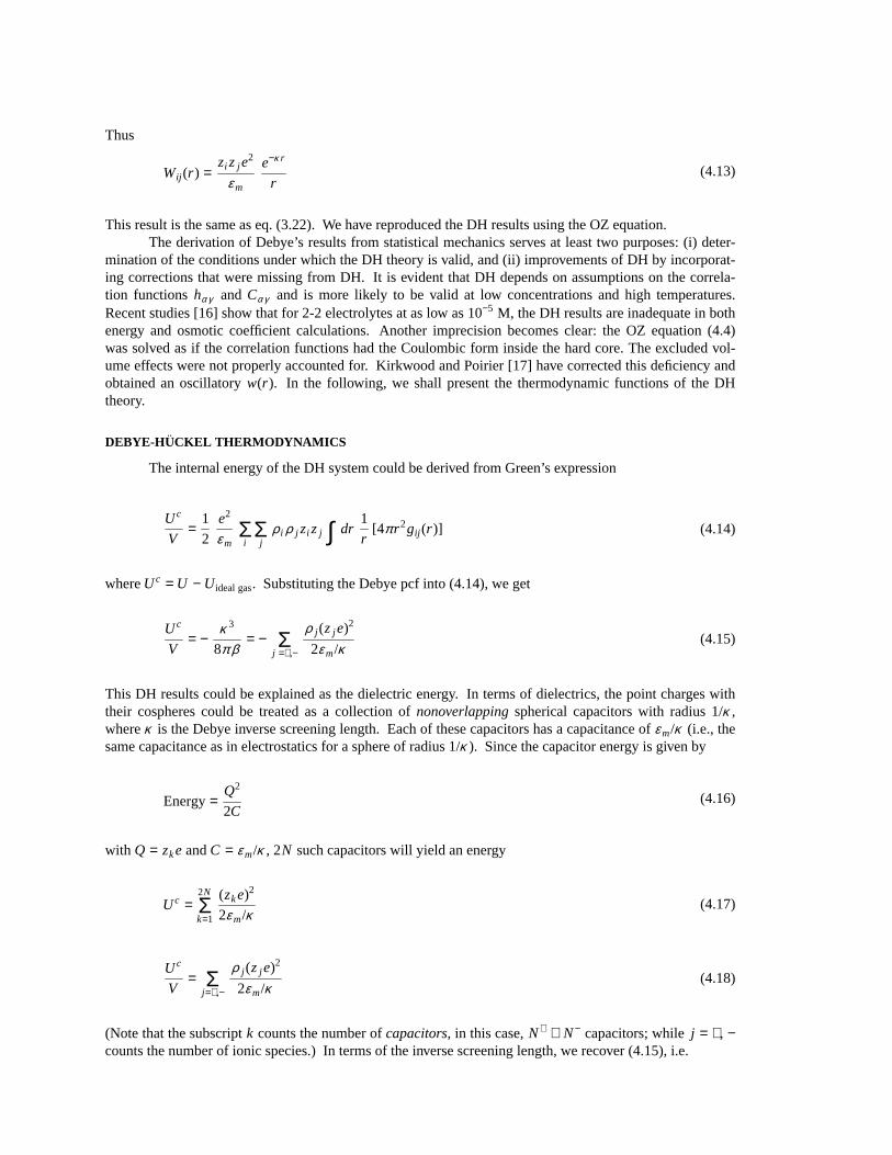
Thus

(4.13)Wij (r ) =zi zj e

2

ε m

e−κ r

r

This result is the same as eq. (3.22). We hav e reproduced the DH results using the OZ equation.The derivation of Debye’s results from statistical mechanics serves at least two purposes: (i) deter-

mination of the conditions under which the DH theory is valid, and (ii) improvements of DH by incorporat-ing corrections that were missing from DH. It is evident that DH depends on assumptions on the correla-tion functionshαγ and Cαγ and is more likely to be valid at low concentrations and high temperatures.Recent studies [16] show that for 2-2 electrolytes at as low as 10−5 M, the DH results are inadequate in bothenergy and osmotic coefficient calculations. Another imprecision becomes clear: the OZ equation (4.4)was solved as if the correlation functions had the Coulombic form inside the hard core. The excluded vol-ume effects were not properly accounted for. Kirkwood and Poirier [17] have corrected this deficiency andobtained an oscillatoryw(r ). In the following, we shall present the thermodynamic functions of the DHtheory.

DEBYE-HUCKEL THERMODYNAMICS

The internal energy of the DH system could be derived from Green’s expression

(4.14)Uc

V=

1

2

e2

ε m iΣ

jΣ ρ i ρ j zi zj ∫ dr

1

r[4π r 2gij (r )]

whereUc = U − Uideal gas. Substituting the Debye pcf into (4.14), we get

(4.15)Uc

V= −

κ 3

8π β= −

j =+,−Σ

ρ j (zj e)2

2ε m/κ

This DH results could be explained as the dielectric energy. In terms of dielectrics, the point charges withtheir cospheres could be treated as a collection ofnonoverlappingspherical capacitors with radius 1/κ ,whereκ is the Debye inverse screening length. Each of these capacitors has a capacitance ofε m/κ (i.e., thesame capacitance as in electrostatics for a sphere of radius 1/κ ). Since the capacitor energy is given by

(4.16)Energy=Q2

2C

with Q = zke andC = ε m/κ , 2N such capacitors will yield an energy

(4.17)Uc =2N

k=1Σ (zke)2

2ε m/κ

(4.18)Uc

V=

j=+,−Σ

ρ j (zj e)2

2ε m/κ

(Note that the subscriptk counts the number ofcapacitors, in this case,N+ + N− capacitors; whilej = +, −counts the number of ionic species.) In terms of the inverse screening length, we recover (4.15), i.e.

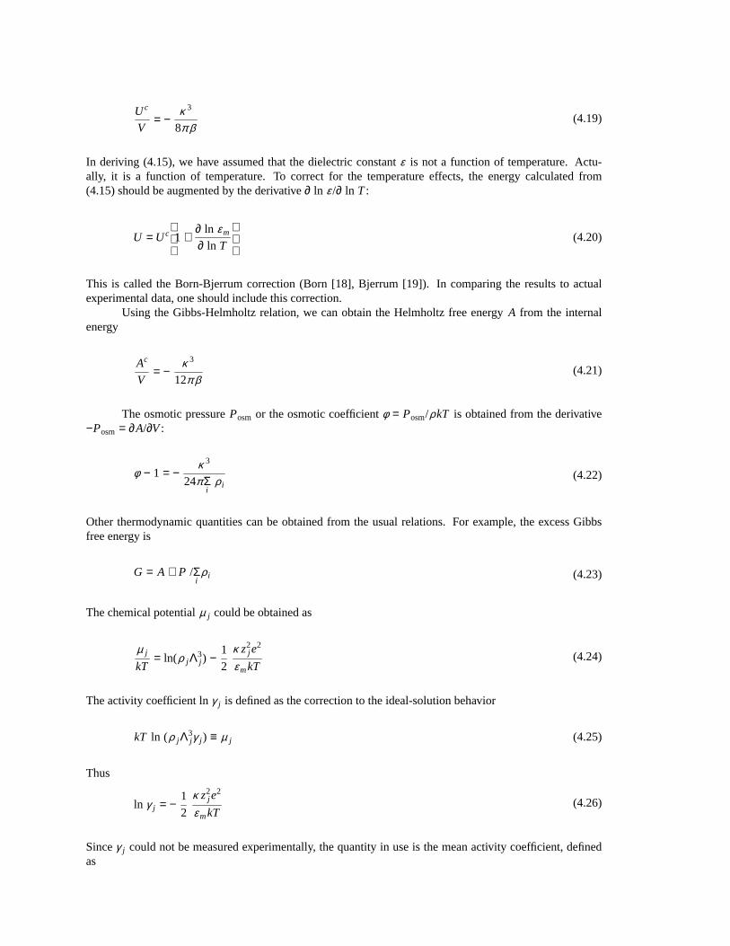
(4.19)Uc

V= −

κ 3

8π β

In deriving (4.15), we have assumed that the dielectric constantε is not a function of temperature. Actu-ally, it is a function of temperature. To correct for the temperature effects, the energy calculated from(4.15) should be augmented by the derivative∂ ln ε /∂ ln T:

(4.20)U = Uc1 +

∂ ln ε m

∂ ln T

This is called the Born-Bjerrum correction (Born [18], Bjerrum [19]). In comparing the results to actualexperimental data, one should include this correction.

Using the Gibbs-Helmholtz relation, we can obtain the Helmholtz free energyA from the internalenergy

(4.21)Ac

V= −

κ 3

12π β

The osmotic pressurePosm or the osmotic coefficientφ = Posm/ρkT is obtained from the derivative−Posm = ∂A/∂V:

(4.22)φ − 1 = −κ 3

24πiΣ ρ i

Other thermodynamic quantities can be obtained from the usual relations. For example, the excess Gibbsfree energy is

(4.23)G = A + P /iΣρ i

The chemical potentialµ j could be obtained as

(4.24)µ j

kT= ln(ρ j Λ3

j ) −1

2

κ z2j e

2

ε mkT

The activity coefficient lnγ j is defined as the correction to the ideal-solution behavior

(4.25)kT ln (ρ j Λ3jγ j ) ≡ µ j

Thus

(4.26)ln γ j = −1

2

κ z2j e

2

ε mkT

Sinceγ j could not be measured experimentally, the quantity in use is the mean activity coefficient, definedas

(4.27)ln γ± ≡ν+ ln γ+ + ν− ln γ−

ν+ + ν −

whereν+ andν− are stoichiometric coefficients of dissociation

(4.28)Cν+Aν−

→ ν+Cz+ + ν− Az−

whereC is the cation andA is the anion. For example, Na3PO4 → 3Na+ + PO−34 , ν+ = 3 andν− = 1. γ± is

a stoichiometrically averaged activity coefficient. From (4.26), we have

(4.29)ln γ± = β Gc = −κ2

β e2

ε m|z+z−|

Thus the mean activity coefficient is proportional to the square root of the ionic strengthI . A typi-cal activity coefficient curve is shown in Figure XII.1 for NaCl up to saturation (at 5∼6 M). The logarith-mic curve first drops below zero then changes sign at higher concentrations. The linear Debye-H¨uckelregion is confined to lowI (roughly less than 0.01 M). It is grossly inadequate at higher concentrations.

XII.5 . Mean Spherical Approximation in the Restricted Primitive Model

We hav e discussed the DH theory at considerable length. However, the utility of the theory is lim-ited. Significant advances occurred in the early l970s when the MSA was solved for the restricted primitivemodel (RPM) of electrolytes. The anions and cations in RPM are charged hard spheres of equal size. Thusthe pair potential is

(5.1)uij (r ) = + ∞, r < d

=qi q j

ε mr, r > d

wherei , j = +, −, qj = zj e, andd is the common diameter of the hard spheres. The MSA assumes that

(5.2)gij (r ) = 0, r < d

Cij (r ) ≈ −qi q j

ε mkT

1

r, r > d

These correlation functions are related by the OZ relation (4.1). Going to Laplace space, Waisman andLebowitz [20] have solved for the dcfCij (r )

(5.3)Cij (r ) = CHSij (r ) −

qi q j

ε mkTd2τ −

τ 2r

d, r < d

= −qi q j

ε mkTr, r > d

where

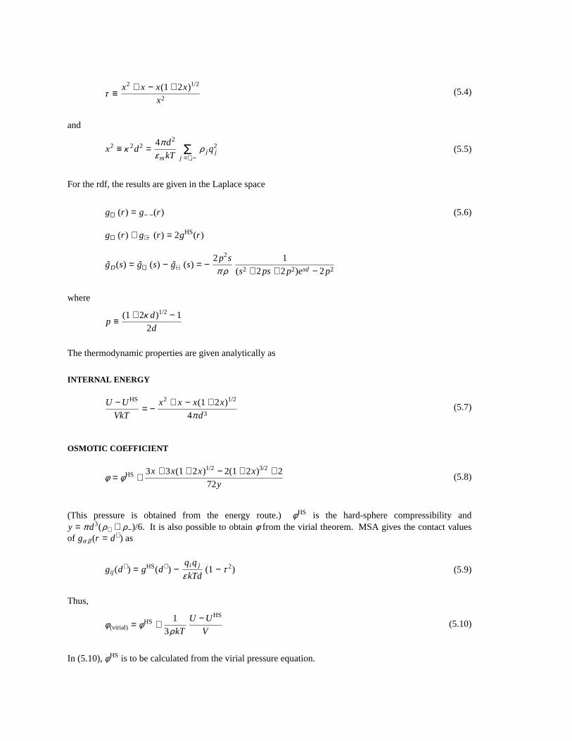
(5.4)τ ≡x2 + x − x(1 + 2x)1/2

x2

and

(5.5)x2 ≡ κ 2d2 =4π d2

ε mkT j =+,−Σ ρ j q

2j

For the rdf, the results are given in the Laplace space

(5.6)g++(r ) = g− −(r )

g++(r ) + g+ −(r ) = 2gHS(r )

gD(s) = g++(s) − g+−(s) = −2p2s

π ρ1

(s2 + 2ps + 2p2)esd − 2p2

where

p ≡(1 + 2κ d)1/2 − 1

2d

The thermodynamic properties are given analytically as

INTERNAL ENERGY

(5.7)U − UHS

VkT= −

x2 + x − x(1 + 2x)1/2

4π d3

OSMOTIC COEFFICIENT

(5.8)φ = φHS +3x + 3x(1 + 2x)1/2 − 2(1+ 2x)3/2 + 2

72y

(This pressure is obtained from the energy route.)φHS is the hard-sphere compressibility andy = π d3(ρ+ + ρ−)/6. It is also possible to obtainφ from the virial theorem. MSA gives the contact valuesof gα β (r = d+) as

(5.9)gij (d+) = gHS(d+) −

qi q j

ε kTd(1 − τ 2)

Thus,

(5.10)φ (virial) = φHS +1

3ρkT

U − UHS

V

In (5.10),φHS is to be calculated from the virial pressure equation.

HELMHOLTZ FREE ENERGY

(5.11)A − AHS

VkT= −

3x2 + 6x + 2 − 2(1+ 2x)3/2

12π d3

It is also clear that the MSA results reduce to the DH values as the diameterd →0. For example, asd → 0the quantity,p approachesκ/2 and the structure

(5.12)d→0lim gD(s) = −

κ 2

2π ρ(s + κ )

This corresponds to the DH rdf of (3.23). Table XII.1 compares the thermodynamic properties of a 1-1electrolyte solution with MC data of Card and Valleau [21] at low concentrations (up to 2 M). MSA givessatisfactory results. The energy values obtained from the MSA are especially accurate. Table XII.2 [22]compares the excess energyUc/(NkT) with MC results at high Bjerrum length. The MSA energy is againshown to be satisfactory at high densities and ionic strength. For the correlation functions, Hirata andArakawa [23] as well as Henderson and Smith [24] have calculatedgij (r ) in real space using zonal repre-sentations. However, comparison with MC results gav e poor agreement. MSAg++(r ) turned negative athigh ionic strengths, an unphysical behavior. Thus MSA is not reliable for structural calculations.

Table XII.1. Osmotic Coefficients and Energies of 1-1 Electrolytes

Conc. φ = β Posm/ρ βU /ρ(moles/l) MC MSA PY HNC MC MSA PY HNC

0.00911 0.970 0.969 0.970 0.970 0.103 0.099 0.101 0.1010.10376 0.945 0.931 0.946 0.946 0.274 0.268 0.271 0.2710.425 0.977 0.945 0.984 0.980 0.434 0.426 0.429 0.4291.00 1.094 1.039 1.108 1.091 0.552 0.541 0.542 0.5451.968 1.346 1.276 1.386 1.340 0.651 0.636 0.638 0.646

Table XII.2. Energies at High Bjerrum Lengths for RPM Salts

Excess Energy,−Uc/VkTρ * B/d− − MC MSA HNC

0.2861 1.8823 0.839 0.804 0.8329.4111 5.465 5.278 5.431

47.055 33.62 31.87 -0.4788 1.5873 0.783 0.725 0.767

7.9368 4.876 4.664 4.85939.684 28.61 27.75 28.66

0.669 1.4191 0.756 0.675 0.7317.0952 4.601 4.288 4.540

35.476 26.54 25.28 26.200.7534 1.3634 0.711 0.657 0.719

6.8172 4.511 4.16 4.34334.0859 25.71 24.45 25.46

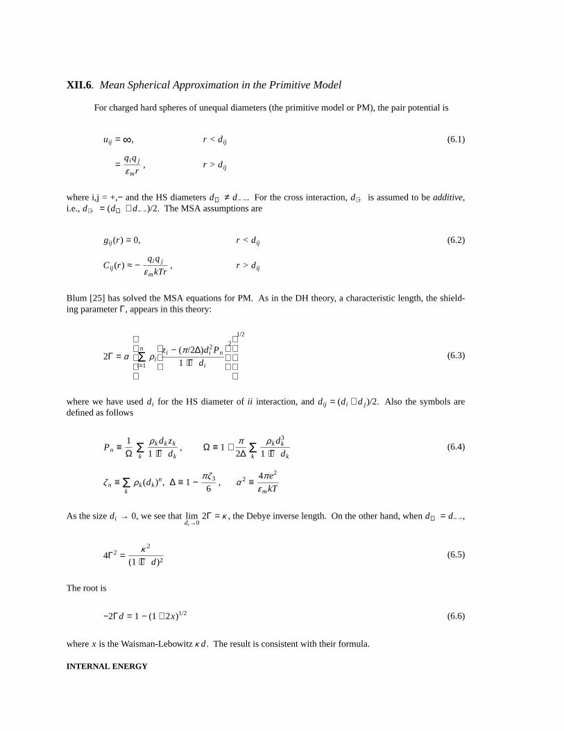
XII.6 . Mean Spherical Approximation in the Primitive Model

For charged hard spheres of unequal diameters (the primitive model or PM), the pair potential is

(6.1)uij = ∞, r < dij

=qi q j

ε mr, r > dij

where i,j = +,− and the HS diametersd++ ≠ d− −. For the cross interaction,d+ − is assumed to beadditive,i.e., d+ − = (d++ + d− −)/2. The MSA assumptions are

(6.2)gij (r ) = 0, r < dij

Cij (r ) ≈ −qi q j

ε mkTr, r > dij

Blum [25] has solved the MSA equations for PM. As in the DH theory, a characteristic length, the shield-ing parameterΓ, appears in this theory:

(6.3)2Γ = α

n

i=1Σ ρ i

zi − (π /2∆)d2i Pn

1 + Γdi

2

1/2

where we have useddi for the HS diameter ofii interaction, anddij = (di + d j )/2. Also the symbols aredefined as follows

(6.4)Pn ≡1

Ω kΣ ρ kdkzk

1 + Γdk, Ω ≡ 1 +

π2∆ k

Σ ρ kd3k

1 + Γdk

ζ n ≡kΣ ρ k(dk)n, ∆ ≡ 1 −

πζ3

6, α 2 ≡

4π e2

ε mkT

As the sizedi → 0, we see thatdi →0lim 2Γ = κ , the Debye inverse length. On the other hand, whend++ = d− −,

(6.5)4Γ2 =κ 2

(1 + Γd)2

The root is

(6.6)−2Γd = 1 − (1 + 2x)1/2

wherex is the Waisman-Lebowitzκ d. The result is consistent with their formula.

INTERNAL ENERGY

(6.7)−U − UHS

VkT=

e2

ε mkT

Γ

n

i=1Σ ρ i z

2i

1 + Γdi+

π2∆

ΩP2n

HELMHOLTZ FREE ENERGY

(6.8)A − AHS

VkT=

U − UHS

VkT+

Γ3

3π

OSMOTIC COEFFICIENT

(6.9)φ − φHS = −Γ3

3π ρ−

α 2

8ρ

Pn

∆

2

MEAN ACTIVITY COEFFICIENT

(6.10)ln γ± − ln γ HS± =

U − UHS

NkT−

α 2

8ρ

Pn

∆

2

INVERSE ISOTHERMAL COMPRESSIBILITY

(6.11)β∂P

∂ρ

T

=1

4ζ0π 2

n

j=1Σ ρ jQ

2j

where

(6.12)Qj =2π∆

1 + ζ2d j

π2∆

+1

2aj Pn

and

(6.13)aj =α 2

2Γ(1 + Γd j )zj − Pn d2

jπ2∆

DIRECT CORRELATION FUNCTIONS

For r > (di + d j )/2, Cij (r ) is giv en by the MSA assumption (6.2). Forr < (di + d j )/2, we divide theregion into two parts, "A": 0≤ r ≤ (d j − di )/2 ≡ x, and "B": (d j − di )/2 ≤ r ≤ (di + d j )/2 ≡ y, (assumingthatdi < d j ).

| | |0 x y

Region "A" Region "B"

ForC++ andC− −, region "A" is nonexistent. In region "A",

(6.14)Cij (r ) = C(0)ij (r ) −

2e2

ε mkT

− zi N j + Xi (Ni + ΓXi ) −di

3(Ni + ΓXi )

2

whereC(0)ij (r ) are the dcfs in the HS mixture. The new parameters are

(6.15)Xi ≡zi − (π /2∆) d2

i Pn

1 + Γdi

and

(6.16)− Ni ≡zi Γ + (π /2∆) di Pn

1 + Γdi

Thus

(6.17)Ni + ΓXi = −π2∆

di Pn

In region "B", the dcfs are given by

(6.18)rCij (r ) − rC (0)ij (r ) =

e2

ε mkT⋅ . . .

RADIAL DISTRIBUTION FUNCTIONS

For the rdf, the contact values are given by

(6.19)dij gij (dij ) =dij

1 − ξ3+

3

2

ξ2di d j

(1 − ξ3)2−

e2Xi X j

ε mkT

For the rdf atr > (di + d j )/2, the expressions are given in the Laplace space by Blum and H/oye [26]. It isof the form

(6.20)gij (s) =D0D±

DTg0

ij (s) −D0Γ2

sα 2π DTe−sσ ij ai a j + ∆gij (s)

Here, the first term, aside from a factor, giv es essentially the PY solution for a pure HS mixture, the secondterm is purely electrostatic in nature, and the third term is derived from the cross interaction between thehard core and the electric charges. The algebraic expressions of these terms have been given by Blum andH/oye (Ibid.) and will not be repeated here. However, for PM at low concentrations, Blum showed that asPn ≈ 0 (this happens whendi = d j or whenρd3

j ≤ 0. 1), the Laplace transform ofgij is

(6.21)gij (s) ≈ gHSij (s) − Aij e−sdij

s2 + 2Γs + 2Γ2 −

2Γ2

α 2mΣ ρ ma2

me−sdm

−1

whereaj has been defined in eq. (6.13), and

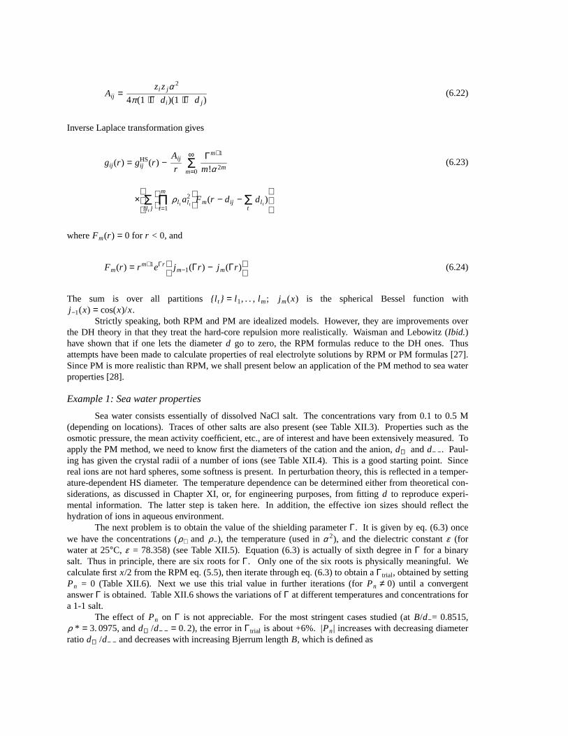
(6.22)Aij =zi zjα

2

4π (1 + Γdi )(1 + Γd j )

Inverse Laplace transformation gives

(6.23)gij (r ) = gHSij (r ) −

Aij

r

∞

m=0Σ Γm+1

m!α 2m

×l t Σ

m

t=1Π ρ l t

a2l t

Fm(r − dij −

tΣ dl t

)

whereFm(r ) = 0 for r < 0, and

(6.24)Fm(r ) = r m+1eΓr

j m−1(Γr ) − j m(Γr )

The sum is over all partitionsl t = l1, . . , l m; j m(x) is the spherical Bessel function withj−1(x) = cos(x)/x.

Strictly speaking, both RPM and PM are idealized models. However, they are improvements overthe DH theory in that they treat the hard-core repulsion more realistically. Waisman and Lebowitz (Ibid.)have shown that if one lets the diameterd go to zero, the RPM formulas reduce to the DH ones. Thusattempts have been made to calculate properties of real electrolyte solutions by RPM or PM formulas [27].Since PM is more realistic than RPM, we shall present below an application of the PM method to sea waterproperties [28].

Example 1: Sea water properties

Sea water consists essentially of dissolved NaCl salt. The concentrations vary from 0.1 to 0.5 M(depending on locations). Traces of other salts are also present (see Table XII.3). Properties such as theosmotic pressure, the mean activity coefficient, etc., are of interest and have been extensively measured. Toapply the PM method, we need to know first the diameters of the cation and the anion,d++ andd− −. Paul-ing has given the crystal radii of a number of ions (see Table XII.4). This is a good starting point. Sincereal ions are not hard spheres, some softness is present. In perturbation theory, this is reflected in a temper-ature-dependent HS diameter. The temperature dependence can be determined either from theoretical con-siderations, as discussed in Chapter XI, or, for engineering purposes, from fittingd to reproduce experi-mental information. The latter step is taken here. In addition, the effective ion sizes should reflect thehydration of ions in aqueous environment.

The next problem is to obtain the value of the shielding parameterΓ. It is giv en by eq. (6.3) oncewe have the concentrations (ρ+ and ρ−), the temperature (used inα 2), and the dielectric constantε (forwater at 25°C, ε = 78.358) (see Table XII.5). Equation (6.3) is actually of sixth degree inΓ for a binarysalt. Thus in principle, there are six roots forΓ. Only one of the six roots is physically meaningful. Wecalculate firstx/2 from the RPM eq. (5.5), then iterate through eq. (6.3) to obtain aΓtrial, obtained by settingPn = 0 (Table XII.6). Next we use this trial value in further iterations (forPn ≠ 0) until a convergentanswerΓ is obtained. Table XII.6 shows the variations ofΓ at different temperatures and concentrations fora 1-1 salt.

The effect ofPn on Γ is not appreciable. For the most stringent cases studied (atB/d−= 0.8515,ρ * = 3. 0975, andd++/d− − = 0. 2), the error inΓtrial is about +6%. |Pn| increases with decreasing diameterratio d++/d− − and decreases with increasing Bjerrum lengthB, which is defined as

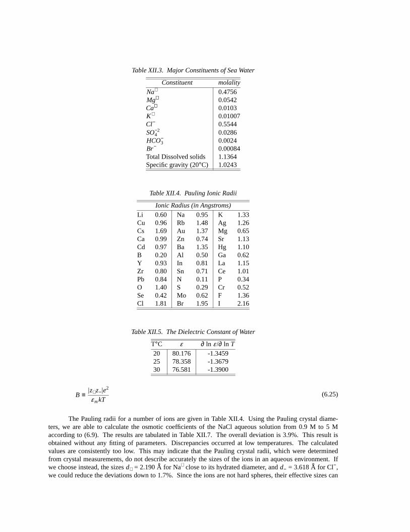
Table XII.3. Major Constituents of Sea Water

Constituent molality

Na+ 0.4756Mg++ 0.0542Ca++ 0.0103K+ 0.01007Cl− 0.5544SO−2

4 0.0286HCO−

3 0.0024Br− 0.00084Total Dissolved solids 1.1364Specific gravity (20°C) 1.0243

Table XII.4. Pauling Ionic Radii

Ionic Radius (in Angstroms)

Li 0.60 Na 0.95 K 1.33Cu 0.96 Rb 1.48 Ag 1.26Cs 1.69 Au 1.37 Mg 0.65Ca 0.99 Zn 0.74 Sr 1.13Cd 0.97 Ba 1.35 Hg 1.10B 0.20 Al 0.50 Ga 0.62Y 0.93 In 0.81 La 1.15Zr 0.80 Sn 0.71 Ce 1.01Pb 0.84 N 0.11 P 0.34O 1.40 S 0.29 Cr 0.52Se 0.42 Mo 0.62 F 1.36Cl 1.81 Br 1.95 I 2.16

Table XII.5. The Dielectric Constant of Water

T°C ε ∂ ln ε /∂ ln T

20 80.176 -1.345925 78.358 -1.367930 76.581 -1.3900

(6.25)B ≡|z+z−|e2

ε mkT

The Pauling radii for a number of ions are given in Table XII.4. Using the Pauling crystal diame-ters, we are able to calculate the osmotic coefficients of the NaCl aqueous solution from 0.9 M to 5 Maccording to (6.9). The results are tabulated in Table XII.7. The overall deviation is 3.9%. This result isobtained without any fitting of parameters. Discrepancies occurred at low temperatures. The calculatedvalues are consistently too low. This may indicate that the Pauling crystal radii, which were determinedfrom crystal measurements, do not describe accurately the sizes of the ions in an aqueous environment. Ifwe choose instead, the sizesd+ = 2.190 A° for Na+ close to its hydrated diameter, andd− = 3.618 A° for Cl−,we could reduce the deviations down to 1.7%. Since the ions are not hard spheres, their effective sizes can

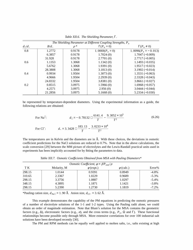
Table XII.6. The Shielding Parameter,Γ.

The Shielding Parameter at Different Coupling Strengths, Pn

d+/d− B/d− ρ * Γ(Pn = 0) Γ(Pn ≠ 0)

0.8 1.2772 0.9178 1. 0069(Pn = 0) 1. 0096(Pn = − 0. 013)6.3857 0.9178 1.7024 (0) 1.7047 (−0.009)

31.928 0.9178 2.7701 (0) 2.7717 (−0.005)0.6 1.1353 1.3068 1.1342 (0) 1.1493 (−0.035)

5.6762 1.3068 1.9391 (0) 1.9517 (−0.023)28.3808 1.3068 3.1813 (0) 3.1902 (−0.014)

0.4 0.9934 1.9504 1.3073 (0) 1.3531 (−0.063)4.9666 1.9504 2.2939 (0) 2.3328 (−0.043)

24.8332 1.9504 3.8381 (0) 3.8661 (−0.027)0.2 0.8515 3.0975 1.5966 (0) 1.6968 (−0.057)

4.2571 3.0975 2.956 (0) 3.0444 (−0.044)21.2856 3.0975 5.1668 (0) 5.2334 (−0.030)

be represented by temperature-dependent diameters. Using the experimental information as a guide, thefollowing relations are obtained:

(6.26)For Na+: d+ = − 0. 78132+6141. 4

T−

9. 3052× 105

T2

For Cl−: d− = 3. 3428+183. 13

T−

3. 0233× 104

T2

The temperatures are in Kelvin and the diameters are in A° . With these choices, the deviations in osmoticcoefficient predictions for the NaCl solutions are reduced to 0.7%. Note that in the above calculations, thescale conversion [29] between the MM picture of electrolytes and the Lewis-Randall practical units used inexperiments has been implicitly accounted for by fitting the parameters to data.

Table XII.7. Osmotic Coefficients Obtained from MSA with Pauling Diameters*

Osmotic Coefficient,φ = β Posm/ρT K Molarity, M φ (expt.) φ (calc.) Error%

298.15 1.0144 0.9391 0.8949 -4.8%310.65 2.3367 1.0229 0.9689 -5.3%298.15 3.3756 1.0887 1.0297 -5.4%348.15 4.3895 1.1871 1.1421 -3.8%298.15 5.2390 1.2730 1.1819 -7.2%

*Pauling cation size,dNa+ = 1. 90 A° . Anion size,dCl− = 3. 62 A° .

This example demonstrates the capability of the PM equations in predicting the osmotic pressuresof a number of electrolyte solutions of the 1-1 and 1-2 types. Using the Pauling radii alone, we couldobtain an order of magnitude estimation. Note that Blum’s solution for the MSA contains the geometricfactors (e.g.,∆), electrostatic factors (e.g.,α), and the cross terms (e.g.,Pn, Ω and Γ). These functionalrelationships become possible only through MSA. More extensive correlations for over 100 industrial saltsolutions have been developed recently [30].

The PM and RPM methods can be equally well applied to molten salts, i.e., salts existing at high

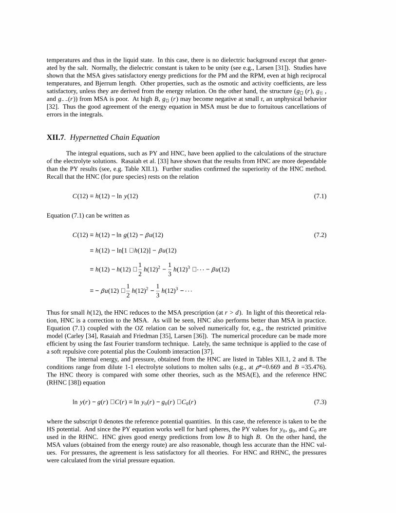
temperatures and thus in the liquid state. In this case, there is no dielectric background except that gener-ated by the salt. Normally, the dielectric constant is taken to be unity (see e.g., Larsen [31]). Studies haveshown that the MSA gives satisfactory energy predictions for the PM and the RPM, even at high reciprocaltemperatures, and Bjerrum length. Other properties, such as the osmotic and activity coefficients, are lesssatisfactory, unless they are derived from the energy relation. On the other hand, the structure (g++(r ), g+−,andg− −(r )) from MSA is poor. At highB, g++(r ) may become negative at small r, an unphysical behavior[32]. Thus the good agreement of the energy equation in MSA must be due to fortuitous cancellations oferrors in the integrals.

XII.7 . Hypernetted Chain Equation

The integral equations, such as PY and HNC, have been applied to the calculations of the structureof the electrolyte solutions. Rasaiah et al. [33] have shown that the results from HNC are more dependablethan the PY results (see, e.g. Table XII.1). Further studies confirmed the superiority of the HNC method.Recall that the HNC (for pure species) rests on the relation

(7.1)C(12) = h(12) − ln y(12)

Equation (7.1) can be written as

(7.2)C(12) = h(12) − ln g(12) − β u(12)

= h(12) − ln[1 + h(12)] − β u(12)

= h(12) − h(12) +1

2h(12)2 −

1

3h(12)3 + . . . − β u(12)

= − β u(12) +1

2h(12)2 −

1

3h(12)3 − . . .

Thus for smallh(12), the HNC reduces to the MSA prescription (atr > d). In light of this theoretical rela-tion, HNC is a correction to the MSA. As will be seen, HNC also performs better than MSA in practice.Equation (7.1) coupled with the OZ relation can be solved numerically for, e.g., the restricted primitivemodel (Carley [34], Rasaiah and Friedman [35], Larsen [36]). The numerical procedure can be made moreefficient by using the fast Fourier transform technique. Lately, the same technique is applied to the case ofa soft repulsive core potential plus the Coulomb interaction [37].

The internal energy, and pressure, obtained from the HNC are listed in Tables XII.1, 2 and 8. Theconditions range from dilute 1-1 electrolyte solutions to molten salts (e.g., atρ*=0.669 andB =35.476).The HNC theory is compared with some other theories, such as the MSA(E), and the reference HNC(RHNC [38]) equation

(7.3)ln y(r ) − g(r ) + C(r ) = ln y0(r ) − g0(r ) + C0(r )

where the subscript 0 denotes the reference potential quantities. In this case, the reference is taken to be theHS potential. And since the PY equation works well for hard spheres, the PY values fory0, g0, andC0 areused in the RHNC. HNC gives good energy predictions from lowB to high B. On the other hand, theMSA values (obtained from the energy route) are also reasonable, though less accurate than the HNC val-ues. For pressures, the agreement is less satisfactory for all theories. For HNC and RHNC, the pressureswere calculated from the virial pressure equation.

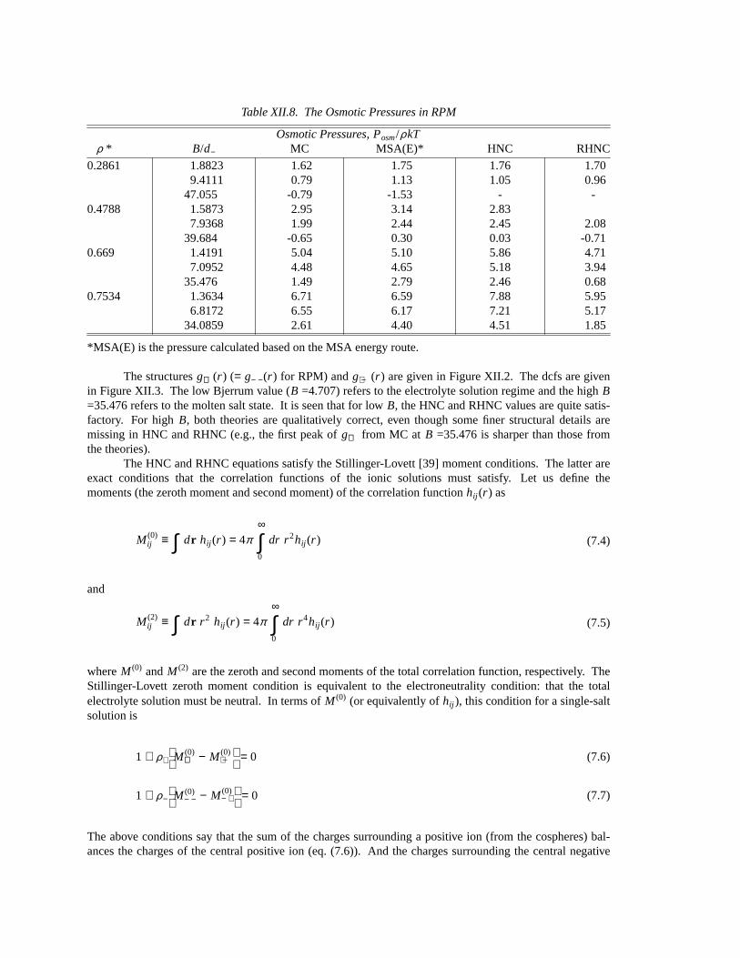
Table XII.8. The Osmotic Pressures in RPM

Osmotic Pressures, Posm/ρkTρ * B/d− MC MSA(E)* HNC RHNC

0.2861 1.8823 1.62 1.75 1.76 1.709.4111 0.79 1.13 1.05 0.96

47.055 -0.79 -1.53 - -0.4788 1.5873 2.95 3.14 2.83

7.9368 1.99 2.44 2.45 2.0839.684 -0.65 0.30 0.03 -0.71

0.669 1.4191 5.04 5.10 5.86 4.717.0952 4.48 4.65 5.18 3.94

35.476 1.49 2.79 2.46 0.680.7534 1.3634 6.71 6.59 7.88 5.95

6.8172 6.55 6.17 7.21 5.1734.0859 2.61 4.40 4.51 1.85

*MSA(E) is the pressure calculated based on the MSA energy route.

The structuresg++(r ) (= g− −(r ) for RPM) andg+ −(r ) are given in Figure XII.2. The dcfs are givenin Figure XII.3. The low Bjerrum value (B =4.707) refers to the electrolyte solution regime and the highB=35.476 refers to the molten salt state. It is seen that for lowB, the HNC and RHNC values are quite satis-factory. For highB, both theories are qualitatively correct, even though some finer structural details aremissing in HNC and RHNC (e.g., the first peak ofg++ from MC at B =35.476 is sharper than those fromthe theories).

The HNC and RHNC equations satisfy the Stillinger-Lovett [39] moment conditions. The latter areexact conditions that the correlation functions of the ionic solutions must satisfy. Let us define themoments (the zeroth moment and second moment) of the correlation functionhij (r ) as

(7.4)M (0)ij ≡ ∫ dr hij (r ) = 4π

∞

0∫ dr r2hij (r )

and

(7.5)M (2)ij ≡ ∫ dr r 2 hij (r ) = 4π

∞

0∫ dr r4hij (r )

whereM (0) andM (2) are the zeroth and second moments of the total correlation function, respectively. TheStillinger-Lovett zeroth moment condition is equivalent to the electroneutrality condition: that the totalelectrolyte solution must be neutral. In terms ofM (0) (or equivalently ofhij ), this condition for a single-saltsolution is

(7.6)1 + ρ+M (0)

++ − M (0)+ −

= 0

(7.7)1 + ρ−M (0)

− − − M (0)− +

= 0

The above conditions say that the sum of the charges surrounding a positive ion (from the cospheres) bal-ances the charges of the central positive ion (eq. (7.6)). And the charges surrounding the central negative

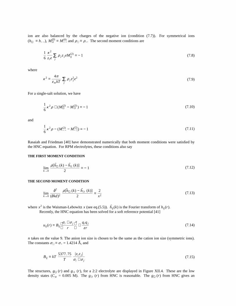
ion are also balanced by the charges of the negative ion (condition (7.7)). For symmetrical ions(h++ = h− −), M (0)

++ = M (0)− − andρ+ = ρ−. The second moment conditions are

(7.8)1

6

κ 2

zi e jΣ ρ j zj eM(2)

ij = − 1

where

(7.9)κ 2 =4π

ε mkT jΣ ρ j z

2j e

2

For a single-salt solution, we have

(7.10)1

6κ 2ρ + (M (2)

++ − M (2)+ −) = − 1

and

(7.11)1

6κ 2ρ − (M (2)

− − − M (2)− +) = − 1

Rasaiah and Friedman [40] have demonstrated numerically that both moment conditions were satisfied bythe HNC equation. For RPM electrolytes, these conditions also say

THE FIRST MOMENT CONDITION

(7.12)k→0lim

ρ[ h++(k) − h+−(k)]

2= − 1

THE SECOND MOMENT CONDITION

(7.13)k→0lim

∂2

(∂kd)2

ρ ˜[h++(k) − h+ −(k)]

2=

2

x2

wherex2 is the Waisman-Lebowitzx (see eq.(5.5)).hij (k) is the Fourier transform ofhij (r ).Recently, the HNC equation has been solved for a soft reference potential [41]

(7.14)uij (r ) = Bij

σ i + σ j

r

n

+qi q j

ε r

n takes on the value 9. The anion ion size is chosen to be the same as the cation ion size (symmetric ions).The constantsσ+ = σ− = 1.4214 A° , and

(7.15)Bij = kT5377. 75

T

|zi zj |

σ i + σ j

The structures,g++(r ) and g+ −(r ), for a 2:2 electrolyte are displayed in Figure XII.4. These are the lowdensity states (Cst = 0.005 M). Theg+ −(r ) from HNC is reasonable. Theg++(r ) from HNC gives an

exaggerated peak atr = 2d. Rossky et al. [42] examined the cause and determined that this exaggerationwas due to the missing bridge diagram (o

•o• ) in the HNC approximation. When the bridge clusters were

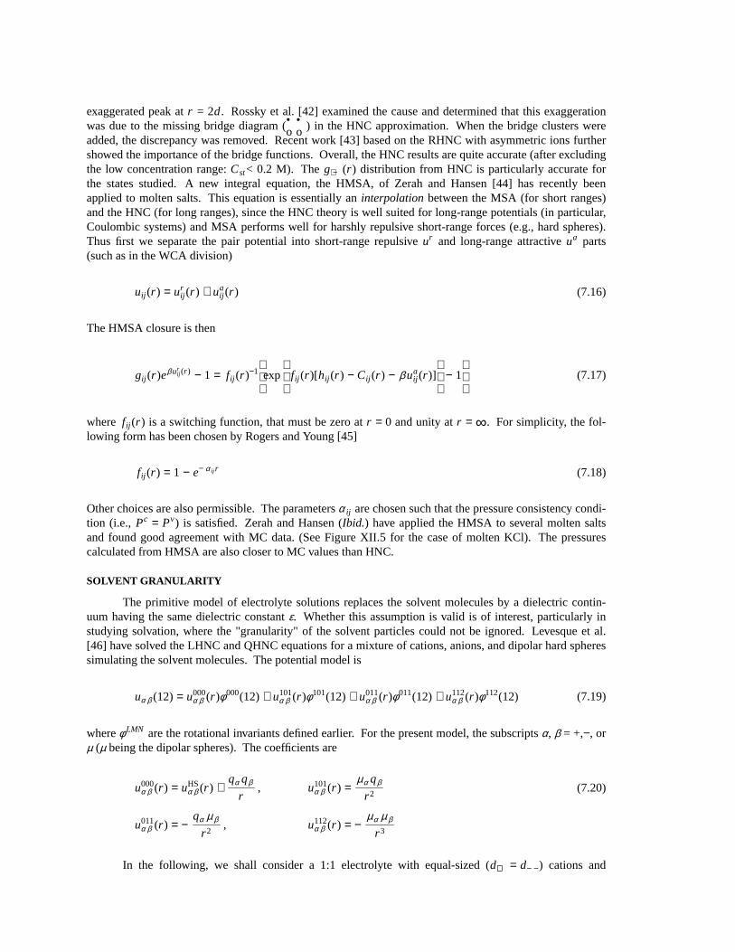
added, the discrepancy was removed. Recent work [43] based on the RHNC with asymmetric ions furthershowed the importance of the bridge functions. Overall, the HNC results are quite accurate (after excludingthe low concentration range:Cst< 0.2 M). Theg+ −(r ) distribution from HNC is particularly accurate forthe states studied. A new integral equation, the HMSA, of Zerah and Hansen [44] has recently beenapplied to molten salts. This equation is essentially aninterpolationbetween the MSA (for short ranges)and the HNC (for long ranges), since the HNC theory is well suited for long-range potentials (in particular,Coulombic systems) and MSA performs well for harshly repulsive short-range forces (e.g., hard spheres).Thus first we separate the pair potential into short-range repulsiveur and long-range attractiveua parts(such as in the WCA division)

(7.16)uij (r ) = urij (r ) + ua

ij (r )

The HMSA closure is then

(7.17)gij (r )eβ urij (r ) − 1 = fij (r )−1

exp

fij (r )[hij (r ) − Cij (r ) − β uaij (r )]

− 1

where fij (r ) is a switching function, that must be zero atr = 0 and unity atr = ∞. For simplicity, the fol-lowing form has been chosen by Rogers and Young [45]

(7.18)fij (r ) = 1 − e− α ij r

Other choices are also permissible. The parametersα ij are chosen such that the pressure consistency condi-tion (i.e., Pc = Pv) is satisfied. Zerah and Hansen (Ibid.) hav e applied the HMSA to several molten saltsand found good agreement with MC data. (See Figure XII.5 for the case of molten KCl). The pressurescalculated from HMSA are also closer to MC values than HNC.

SOLVENT GRANULARITY

The primitive model of electrolyte solutions replaces the solvent molecules by a dielectric contin-uum having the same dielectric constantε. Whether this assumption is valid is of interest, particularly instudying solvation, where the "granularity" of the solvent particles could not be ignored. Levesque et al.[46] have solved the LHNC and QHNC equations for a mixture of cations, anions, and dipolar hard spheressimulating the solvent molecules. The potential model is

(7.19)uα β (12) = u000α β (r )φ000(12) + u101

α β (r )φ101(12) + u011α β (r )φ011(12) + u112

α β (r )φ112(12)

whereφ LMN are the rotational invariants defined earlier. For the present model, the subscriptsα, β = +,−, orµ (µ being the dipolar spheres). The coefficients are

(7.20)u000α β (r ) = uHS

α β (r ) +qα qβ

r, u101

α β (r ) =µα qβ

r 2

u011α β (r ) = −

qα µ β

r 2, u112

α β (r ) = −µα µ β

r 3

In the following, we shall consider a 1:1 electrolyte with equal-sized (d++ = d− −) cations and

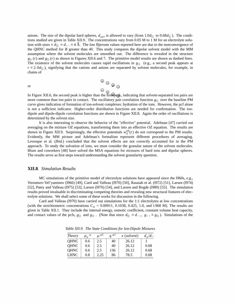
anions. The size of the dipolar hard spheres,dµ µ , is allowed to vary (from 1.0d++ to 0.68d++). The condi-tions studied are given in Table XII.9. The concentrations vary from 0.05 M to 1 M for an electrolyte solu-tion with sizes= d++ = d− − = 4 A° . The low Bjerrum values reported here are due to the nonconvergence ofthe QHNC method forB greater than 40. This study compares the dipolar solvent model with the MMassumption where the solvent molecules are smoothed out. The difference is revealed in the structureg+−(r ) andg++(r ) as shown in Figures XII.6 and 7. The primitive model results are shown as dashed lines.The existence of the solvent molecules causes rapid oscillations ing+ − (e.g., a second peak appears atr = 2. 0d++), signifying that the cations and anions are separated by solvent molecules, for example, inchains of

+ − µ −or− + µ +In Figure XII.6, the second peak is higher than the first peak, indicating that solvent-separated ion pairs are

more common than ion pairs in contact. The oscillatory pair correlation functiong++ over the baseline PMcurve giv es indication of formation of ion-solvent complexes: hydration of the ions. However, the pcf aloneis not a sufficient indicator. Higher-order distribution functions are needed for confirmation. The ion-dipole and dipole-dipole correlation functions are shown in Figure XII.8. Again the order of oscillations isdetermined by the solvent size.

It is also interesting to observe the behavior of the "effective" potential. Adelman [47] carried outav eraging on the mixture OZ equations, transforming them into an effective OZ equation. The results areshown in Figure XII.9. Surprisingly, the effective potentialsweff

ij (r ) do not correspond to the PM results.Evidently, the MM picture and Adelman’s formalism represent different procedures of averaging.Levesque et al. (Ibid.) concluded that the solvent effects are not correctly accounted for in the PMapproach. To study the solvation of ions, we must consider the granular nature of the solvent molecules.Blum and coworkers [48] have solved the MSA equations for mixtures of hard ions and dipolar spheres.The results serve as first steps toward understanding the solvent granularity question.

XII.8 . Simulation Results

MC simulations of the primitive model of electrolyte solutions have appeared since the l960s, e.g.,Vorontsov-Vel’yaminov (l966) [49], Card and Valleau (l970) [50], Rasaiah et al. (l972) [51], Larsen (l974)[52], Patey and Valleau (l975) [53], Larsen (l976) [54], and Larsen and Rogde (l980) [55]. The simulationresults proved inv aluable in discriminating competing theories and revealing new structural features of elec-trolyte solutions. We shall select some of these works for discussion in the following.

Card and Valleau (l970) have carried out simulations for the 1:1 electrolytes at low concentrations(with the stoichiometric concentrationsCst = 0.00911, 0.1038, 0.425, 1.0, and l.968 M). The results aregiven in Table XII.1. They include the internal energy, osmotic coefficient, constant volume heat capacity,and contact values of the pcfs,g++ and g+ −. (Note that sinced++ = d− −, g− − = g++). Simulations of the

Table XII.9. The State Conditions for Ion-Dipole Mixtures

Theory ρ µ * µ *2 q *2 ε (solvent) dµ /d+

QHNC 0.6 2.5 40 26.12 1QHNC 0.6 2.5 40 26.12 0.68QHNC 0.6 2.5 136 26.12 0.68LHNC 0.8 2.25 86 78.5 0.68

pcf were also given. Since they were for low concentrations, no special features were discovered.Larsen [56] published a MC study of the RPM including the molten salt region. The results are

summarized in Table XII.10. The quantity

(8.1)CONTACT = 2y [g++(d++) + g+−(d++)]

wherey = π ρd3++/6, (d++ = d− − andd+ − = (d++ + d− −)/2). The Bjerrum length varies from the electrolyte

solution regime (B/d++ = 1.8823) to the molten salt regime (B/d++= 94.1103). One interesting behavior isthat the like and unlike pcfs at highB show formation of clusters (triplets and quadruplets, etc.) larger thanthe pairs (see Figure XII.10). Atr /d++ = 2, g++(r ) shows a narrow peak of size 1.21. This indicates theformation of the triplets +− +.

The correlation functions for the 2:2 electrolytes are given in Figures XII.11 [57]. Various theoreti-cal results (e.g., MSX, HNC, MSA, and YBG equations) are compared. The MSX equation is due to Outh-waite [58], i.e.,

(8.2)gij (r ) = gHSij (r ) exp

Cij /gHS

ij (r )

whereCij is the chain sum [59]. This function is a graph-theoretical entity, i.e., a sum of all graphs thathave at least oneφ -bond and that are chains ofh0 andφ , whereφ (r ) ≡ − β up(r ). For the DH case, it is sim-ply

(8.3)Cij (r ) = −zi zj e

2

ε mkT

e−κ r

r

Figure XII.11 shows a peak ofg++ at r = 8.4 A° (about twice the ionic diameterd++ = 4.2 A° ). This is

Table XII.10. MC Values for High Bjerrum Lengths (Molten Salts)

y Γ −U/NkT gA(d+) gB(d+) CONTACT PV/NkT

0.1498 2.0 0.839 0.64 2.36 0.90 1.625.0 2.467 0.46 3.72 1.25 1.43

49.98 33.62 0.09 31.32 9.41 -0.7999.96 70.16 0.0 63.46 18.99 -3.40

0.2507 2.0 0.783 1.42 3.14 2.28 3.025.0 2.226 0.68 4.20 2.44 2.70

50.04 28.61 0.03 15.70 7.89 -0.65100.09 59.91 0.01 31.76 15.93 -3.04

0.3503 2.0 0.756 2.38 3.75 4.30 5.045.0 2.114 1.40 4.87 4.39 4.69

50.02 26.54 0.09 13.24 9.34 1.49100.03 54.93 0.03 22.34 15.67 -1.64

0.3945 2.0 0.711 2.60 4.94 5.94 6.715.0 2.067 1.94 5.84 6.13 6.44

49.998 25.71 0.21 12.70 10.18 2.6199.996 53.26 0.10 23.28 18.44 1.69

indication of triplet formation. It was estimated that at 0.0625 M, about 8% of the ions are in triplet form.The energy required for the formation of various ion clusters is presented in Table XII.11. Note that theenergies required to form clusters larger than the triplets (e.g., quadruplets) are considerably higher.

SCREENED COULOMB POTENTIAL

In the study of the DH theory, we hav e derived the averaged ("screened") Coulomb potential. Thepair potential among the ions is of the Yukawa type:

(8.4)uij (r ) = ∞, r ≤ dij

=qi q j

ε mr ije−z(r−dij ), r > dij

wherez is a parameter determining the range of interaction. So asz= 0, we shall recover thebareCoulombinteraction. For nonzeroz values, the Yukawa potential is short-ranged. The reasons for studying theYukawa potential on the microscopic level are that

(i) MC simulation can be done accurately in the absence of long-range forces.

(ii) Coulomb interaction results can be recovered asz → 0, thus the simulations have significance forionic solutions.

(iii) As shall become evident shortly, the performance of different theoretical approaches is altered (somegetting better, some getting worse) as the range of intermolecular forces is shortened. For example,in the case of MSA, results deteriorate asz is increased or when the range of interaction is curtailed.

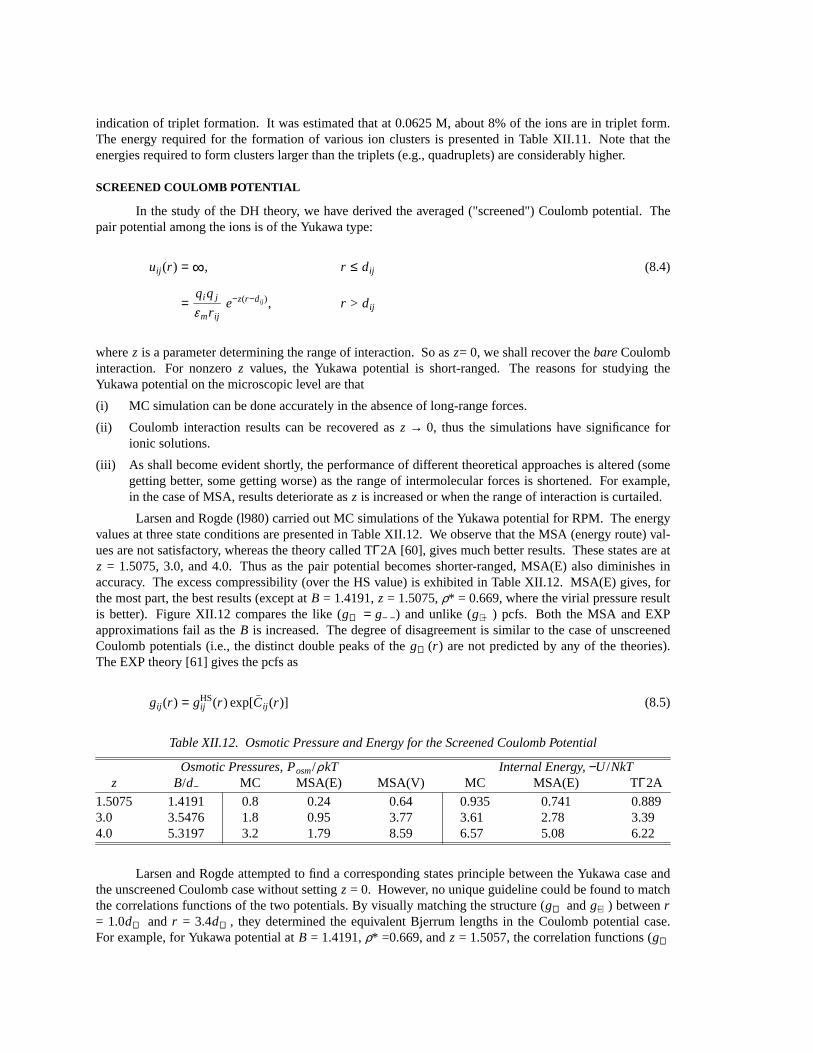
Larsen and Rogde (l980) carried out MC simulations of the Yukawa potential for RPM. The energyvalues at three state conditions are presented in Table XII.12. We observe that the MSA (energy route) val-ues are not satisfactory, whereas the theory called TΓ2A [60], gives much better results. These states are atz = 1.5075, 3.0, and 4.0. Thus as the pair potential becomes shorter-ranged, MSA(E) also diminishes inaccuracy. The excess compressibility (over the HS value) is exhibited in Table XII.12. MSA(E) gives, forthe most part, the best results (except atB = 1.4191,z = 1.5075,ρ* = 0.669, where the virial pressure resultis better). Figure XII.12 compares the like (g++ = g− −) and unlike (g+ −) pcfs. Both the MSA and EXPapproximations fail as theB is increased. The degree of disagreement is similar to the case of unscreenedCoulomb potentials (i.e., the distinct double peaks of theg++(r ) are not predicted by any of the theories).The EXP theory [61] gives the pcfs as

(8.5)gij (r ) = gHSij (r ) exp[Cij (r )]

Table XII.12. Osmotic Pressure and Energy for the Screened Coulomb Potential

Osmotic Pressures, Posm/ρkT Internal Energy,−U /NkTz B/d− MC MSA(E) MSA(V) MC MSA(E) TΓ2A

1.5075 1.4191 0.8 0.24 0.64 0.935 0.741 0.8893.0 3.5476 1.8 0.95 3.77 3.61 2.78 3.394.0 5.3197 3.2 1.79 8.59 6.57 5.08 6.22

Larsen and Rogde attempted to find a corresponding states principle between the Yukawa case andthe unscreened Coulomb case without settingz = 0. Howev er, no unique guideline could be found to matchthe correlations functions of the two potentials. By visually matching the structure (g++ andg+−) betweenr= 1.0d++ and r = 3.4d++, they determined the equivalent Bjerrum lengths in the Coulomb potential case.For example, for Yukawa potential atB = 1.4191,ρ* =0.669, andz = 1.5057, the correlation functions (g++

andg+−) match those of the Coulomb potential atB = 3.5476 andρ* = 0.669 (z=0).

References

[1] J.H. Hildebrand and R.L. Scott,The Solubility of Nonelectrolytes, Third edition (Reinhold, NewYork, 1924).

[2] P. Debye and E. H"uckel, Z. Physik24, 195 and 305 (1923).

[3] H. Falkenhagen,Electrolytes(Oxford University Press, London, 1934).

[4] E. Mayer, J. Chem. Phys.5, 67 (1937); andIbid. 18, 1426 (1950).

[5] N. Bjerrum, K. dan. Vidensk. Selsk.7, No. 9 (1926); andSelected Papers, (Munskgaard, Copen-hagen, 1949).

[6] E.A. Guggenheim, Phil. Mag.19, 588 (1926); and E.A. Guggenheim and J.C. Turgeon, Trans. Fara-day Soc.51, 747 (1955).

[7] W.G. McMillan and J.E. Mayer, J. Chem. Phys.13, 276 (1945).

[8] O. Matsuoka, E. Clementi, and M. Yoshimine, J. Chem. Phys.64, 1351 (1976).

[9] H.C. Andersen and D. Chandler, J. Chem. Phys.55, 1497 (1971); and H.C. Andersen, D. Chandler,and J.D. Weeks,Ibid., 56, 3812 (1972).

[10] G. Stell, inStatistical Mechanics: Equilibrium Techniques, Part A, edited by B.J. Berne (Plenum,New York, 1977), pp.47-84.

[11] A.R. Allnatt, Mol. Phys.8, 533 (1964).

[12] D.D. Carley, J. Chem. Phys.46, 3783 (1967); also J.C. Rasaiah and H.L. Friedman, J. Chem. Phys.48, 2742 (1968).

[13] D.R. Corson and P. Lorrain,Introduction to Electromagnetic Fields and Waves(W.H. Freeman, SanFrancisco, 1962).

[14] H.L. Friedman and W.D.T. Dale, inStatistical Mechanics: Equilibrium Techniques, Part A, edited byB. J. Berne, (Plenum, New York, 1977), pp.85-135.

[15] C.W. Outhwaite, inStatistical Mechanics, edited by K. Singer, (Chemical Society, London, 1975),p.188.

[16] P.J. Rossky, J.B. Dudowicz, B.L. Tembe, and H.L. Friedman, J. Chem. Phys.73, 3372 (1980).

[17] J.G. Kirkwood and J.C. Poirier, J. Phys. Chem.58, 591 (1954).

[18] M. Born, Z. Phys.1, 45 (1920).

[19] N. Bjerrum,Selected Papers, (Munskgaard, Copenhagen, 1949).

[20] E. Waisman and J.L. Lebowitz, J. Chem. Phys.52, 4037 (1970); alsoIbid., 56, 3086 and 3093(1972).

[21] D.N. Card and J.P. Valleau, J. Chem. Phys.52, 6232 (1970).

[22] G. Stell and B. Larsen, J. Chem. Phys.70, 361 (1979).

[23] F. Hirata and K. Arakawa, Bull. Chem. Soc. Japan48, 2139 (1975).

[24] D. Henderson and W.R. Smith, J. Stat. Phys.19, 191 (1978).

[25] L. Blum, Mol. Phys.30, 1529 (1975).

[26] L. Blum and J.S. H/oye, J. Phys. Chem.81, 1311 (1977).

[27] See, e.g., R. Triolo, J.R. Grigera, and L. Blum, J. Phys. Chem.80, 1858 (1976); R. Triolo, L. Blum,and M.A. Floriano, J. Chem. Phys.67, 5956 (1977); and J. Phys. Chem.82, 1368 (1978).

[28] S. Watanasiri, M.R. Brul´e, and L.L. Lee, J. Phys. Chem.86, 292 (1982).

[29] See, e.g., H.L. Friedman, J. Solution Chem.1, 387 (1972).

[30] L.H. Landis, Ph.D. Thesis,Mixed Salt Electrolyte Solutions: Accurate Correlation for Osmotic Coef-ficients Based on Molecular Distribution Functions, University of Oklahoma (1984).

[31] B. Larsen, J. Chem. Phys.65, 3431 (1976).

[32] L.L. Lee, J. Chem. Phys.78, 5270 (1983).

[33] J.C. Rasaiah, D.N. Card, and J.P. Valleau, J. Chem. Phys.56, 248 (1972).

[34] D.D. Carley, J. Chem. Phys.46, 3783 (1967).

[35] J.C. Rasaiah and H.L. Friedman, J. Chem. Phys.48, 2742 (1968).

[36] B. Larsen, J. Chem. Phys.68, 4511 (1978).

[37] P.J. Rossky, J.B. Dudowicz, B.L. Tembe, and H.L. Friedman, J. Chem. Phys.73, 3372 (1980); andR. Bacquet and P.J. Rossky, J. Chem. Phys.79, 1419 (1983).

[38] B. Larsen, J. Chem. Phys.68, 4511 (1978).

[39] F.H. Stillinger and R. Lovett, J. Chem. Phys.48, 3858 and 3869 (1968).

[40] J.C. Rasaiah and H.L. Friedman, J. Chem. Phys.50, 3965 (1969).

[41] P.J. Rossky, J.B. Dudowicz, B.L. Tembe, and H.L. Friedman, J. Chem. Phys.73, 3372 (1980); andR. Bacquet and P.J. Rossky, J. Chem. Phys.79, 1419 (1983).

[42] R. Bacquet and P.J. Rossky,Ibid. (1983).

[43] C. Caccamo, G. Malescio, and L. Reatto, J. Chem. Phys.81, 4093 (1984).

[44] J.P. Hansen and G. Zerah, Phys. Lett.108A, 277 (1985); also G. Zerah and J.P. Hansen, J. Chem.Phys.84, 2336 (1986).

[45] F.J Rogers and D.A. Young, Phys. Rev. A30, 999 (1984).

[46] D. Levesque, J.-J. Weis, and G.N. Patey, J. Chem. Phys.72, 1887 (1980).

[47] S.A. Adelman and J.H. Chen, J. Chem. Phys.70, 4291 (1979).

[48] L. Blum, J. Stat. Phys.18, 451 (1978); F. Vericat and L. Blum,Ibid. 22, 593 (1980); and Mol. Phys.45, 1067 (1982).

[49] P.N. Vorontsov-Vel’yaminov and V.P. Chasovskikh, High Temperatures (USSR)13, 1071 (1975);P.N. Vorontsov-Vel’yaminov, H.M. El’yashevich, and A.K. Kron, Elektrokhimiya2, 708 (1966); alsoP.N. Vorontsov-Vel’yaminov and H.M. El’yashevich,Ibid. 4, 1430 (1968).

[50] D.N. Card and J.P. Valleau, J. Chem. Phys.52, 6323 (1970).

[51] J.C. Rasaiah, D.N. Card, and J.P. Valleau, J. Chem. Phys.56, 248 (1972).

[52] B. Larsen, Chem. Phys. Letters27, 47 (1974).

[53] G.N. Patey and J.P. Valleau, J. Chem. Phys.63, 2334 (1975).

[54] B. Larsen, J. Chem. Phys.65, 3431 (1976).

[55] B. Larsen and S.A. Rogde, J. Chem. Phys.72, 2578 (1980).

[56] B. Larsen,Ibid. (1974).

[57] J.P. Valleau, L.K. Cohen, and D.N. Card, J. Chem. Phys.72, 5942 (1980).

[58] C.W. Outhwaite, Chem. Phys. Lett.37, 383 (1976).

[59] See e.g., H.C. Andersen, inStatistical Mechanics: Equilibrium Techniques, Part A, edited by B.J.Berne (Plenum, New York, 1977)

[60] B. Larsen, G. Stell, and K.C. Wu, J. Chem. Phys.7, 530 (1977).

[61] H.C. Andersen and D. Chandler, J. Chem. Phys.57, 1918 (1972).

[62] R.A. Robinson and R.H. Stokes,Electrolyte Solutions, 2nd Edition (Butterworth, London, 1970).

Exercises

1. Derive the Debye-H¨uckel thermodynamic quantities, such as energy, osmotic pressure, andchemical potential by using the radial distribution functiongij (3.23) in the energy andpressure equations from Chapter V. Check your results against those listed in SectionXII.4.

2. Plot the mean activity coefficient lnγ± at 25°C as a function of ionic strength for NaCl from 0 to 5M,using DH formula. Compare with experimental data (see e.g., Robinson and Stokes [62]). Discussthe deficiencies of the DH theory at high concentrations.

3. Use the fast Fourier transform technique to solve the HNC equation for NaCl solution at the sameconditions. You may use the PM model and the Pauling radii for Na+ and Cl−. Calculate the osmoticpressure from the virial theorem and compare with experimental data. State explicitly the assump-tions made and discuss the results.

4. Two new integral equations, the RHNC and the HMSA, have been proposed. Apply these equationsto the NaCl solution at 25°C and a number of molarities. Compare with the results from the HNCequation.

5. Survey the literature to find alternative theories for the mean activity coefficients of 2:2 electrolytes.Discuss their merits and weaknesses.

6. The hard ion models presented here could equally be applied to molten salts and two-componentplasmas. Consult the literature to find applications of the present theories to these fluids. Discuss thesimilarities to and differences from the electrolyte solutions.