Labor Protection and Leverage

Elena Simintzi∗, Vikrant Vig∗∗ and Paolo Volpin∗∗

December 2012

Abstract

This paper examines the effect of labor protection on firm financial structure.We exploit inter-temporal variations in employment protection laws across 21OECD countries and find that labor friendly reforms are associated with areduction in firm leverage. We also find that the negative effect of labor pro-tection on leverage is more pronounced in firms that rely more on labor, aresubject to more frequent hiring and firing, and have lower liquidation value.These results are consistent with the view that employment protection increasesoperating leverage and thus crowds out financial leverage. Furthermore, we findthat increases in employment protection impact negatively firm investment andgrowth in sectors that are more dependent on external capital. These resultsindicate that firms’ reduced ability to raise external capital, due to strongerlabor protection, has negative real effects.

JEL classification: J31, J51, G32, G33, K31.

Keywords: labor regulation, capital structure, tangibility, operating leverage.

Affiliations: ∗Sauder School of Business, University of British Columbia; ∗∗London Busi-

ness School; e-mails: elena.simintzi@sauder.ubc.ca, vvig@london.edu, pvolpin@london.edu.

Acknowledgments: We would like to thank Gayle Allard, Manuel Arellano, Ulf Ax-

elson, Patrick Bolton, Gilles Chemla, Francesca Cornelli, Andrea Eisfeldt, Julian Franks,

Oliver Hart, Christopher Hennessy, Brandon Julio, David Matsa, Marco Pagano, Enrico

Perotti, Gordon Phillips, Antoinette Schoar, Florian Schulz, Amit Seru, Ilya Strebulaev,

Toni Whited and seminar participants at Boston College, CEMFI, EFA, FIRS, George-

town, IE, LBS, LSE, NBER Corporate Finance Meetings, Ohio State University, Oxford

University, and WFA for helpful discussions and comments.

I Introduction

There is a large literature that shows that frictions such as taxes, bankruptcy costs,

asymmetric information, and agency conflicts have a first order effect on financial con-

tracting decisions of firms. In this paper, we make an attempt to push this literature

forward by taking a stakeholder perspective and examining how labor regulations af-

fect the capital structure of firms.1 Since labor regulations alter the ex-post division

of firm’s proceeds between different stakeholders, it is natural to expect that they

should have a significant impact on the ex-ante financial decisions of firms.

Using firm-level data from 21 countries over the 1985-2004 period, we exploit

inter-temporal variations in employment protection laws across countries, and adopt

a difference-in-differences (DID) research design to investigate the impact of labor

reforms on firm financial structure.2 We find that a one-unit increase in the index of

Employment Protection Legislation (EPL) is associated with a reduction of debt by

4% (in absolute terms) or of 14% (relative to the mean).3

These results are not driven by pre-treatment trends or business cycle effects, or

even by the endogeneity of labor laws themselves.4 Moreover, in addition to the firm

1In this respect we contributed to the growing literature on labor and finance. See Kim (2009)and Pagano (2010) for a survey.

2These changes in regulation represent a near-ideal setting since they are exogenous to theindividual firm.

3Another way of interpreting this finding is that going from a country like Canada (EPL of 1)to a country like Italy (EPL of 3) leverage should decrease by 8% (in absolute terms) or 29% (inrelative terms).

4Examining the dynamics of leverage around the passage of these laws, we find no statisticallysignificant change in leverage prior to the passage of these laws but we find a change in leverage oneand two years after the passage of the laws. This finding alleviates the concerns of reverse causalityand/or pre-treatment trends that may confound the analysis.

– 1 –

and industry-year fixed effects, we contemporaneously control for firm profitability,

size, investment opportunities and tangibility – variables that have been shown to

affect capital structure of firms. In other words, we directly control for capital struc-

ture effects that come through changes in firm level variables, such as changes to firm

level profitability or investment opportunities that is brought about by the labor reg-

ulation. Thus, the effect of labor regulation on capital structure that we document

is independent of the traditional determinants of firms’ capital structure.

What drives this effect? We rationalize these findings with the argument that

employment protection leads to the “debtification” of labor costs: by increasing the

rigidity of labor claims, pro-labor regulations make hiring a worker analogous to

taking on debt where wages can be construed as coupon payment on debt. Further,

because wages usually get paid before other creditors, they are de facto senior to

creditors, in the spirit of Diamond (1993). We argue that this “debtification” of

wages causes operating leverage to crowd out financial leverage. Consistent with this

view, we find that these effects are stronger for more labor intensive firms and firms

for which labor turnover is higher (firms more subject to creative destruction shocks).

The “debtification” channel alluded above, could affect leverage through the de-

mand side and/or the supply side. On the demand side, the greater rigidity of labor

costs may increase the probability of financial distress. To compensate, the firm may

optimally reduce financial leverage. There can, however, be a supply side channel

at work as well. The de facto seniority of labor claims reduces the amount of cash

flows that can be pledged to outside investors, thereby reducing financing capacity

of firms.

– 2 –

We propose a simple model to describe how pro-labor regulation may reduce the

amount of capital that is pledgeable to creditors, or the firm’s debt capacity. The

model builds on the framework proposed by Hart and Moore (1989) and Bolton and

Scharfstein (1990). The key assumption in the model is that debt can force the firm

into liquidation in case of no repayment while dispersed equity cannot. The firm

can thus raise equity only if it invests in a costly state verification technology (which

is a deadweight cost for the firm), which makes cash flows pledgeable to dispersed

shareholders. The firm’s debt capacity is instead determined by the cash flows that

the entrepreneur loses in case of liquidation. These cash flows are pledgeable to

creditors because they can credibly threaten liquidation. The deadweight cost of

raising equity generates a pecking order in financing choices: firms issue equity only

if they have exhausted their debt capacity. Since an increase in labor protection

reduces the cash flows from continuation (as it increases labor bargaining power),

debt capacity decreases with labor protection. As labor protection increases (and

debt capacity decreases), the firm is forced to raise equity to meet their investment

needs. Therefore, the model predicts that leverage decreases with labor protection.

A large increase in labor protection may even lead to underinvestment when the firm

has not enough internal resources, or issuing outside equity is very costly.

The model delivers some interesting cross-sectional implications. First, the model

predicts a differential effect of labor protection on leverage depending on how creditors

fare in liquidation: labor-friendly laws should decrease leverage less in industries

with more tangible assets and countries with stronger creditor protection, which are

proxies for higher liquidation values. Consistent with this prediction, we find that

– 3 –

labor-friendly laws decrease leverage less in industries with more tangible assets and

countries with stronger creditor protection, which are proxies for higher liquidation

values. The effect of a one-standard deviation increase in tangibility on leverage is

1.6% higher in a country with an EPL of 3 (like Italy) compared with a country with

an EPL of 1 (like Canada).

Second, consistent with the model, we show that the effects of employment pro-

tection on firms’ leverage have the real consequence of reducing growth. We find

that the increase in EPL is associated with a reduction in sales’ growth and capital

expenditure in firms dependent on external capital. These firms need to access exter-

nal capital markets in order to invest and are identified following Rajan and Zingales

(1998). The effect of a one-standard deviation increase in external dependence on

sales growth is 2.8% higher in a country with EPL equal to 3 (like Italy) compared

with a country with an EPL of 1 (like Canada). These findings that increases in

EPL reduce investment only in firms with greater dependence on external capital is

supportive of our supply side argument.

These cross-sectional results are also useful since they further address concerns

about potential omitted variables. While our identification strategy (DID) mitigates

some of the concerns about omitted variables, it is possible that our results may

be due to other contemporaneous reforms (such as changes in taxation or corporate

governance reforms). If this were the case, we would incorrectly attribute the changes

in leverage to changes in labor laws. Such effects would be however differenced out in

our cross- sectional heterogeneity specifications. Also, in such a setup we can control

for interacted year and country fixed effects, therefore controlling for any differences

– 4 –

in the regulatory environment over time and across countries.

This paper connects several strands of literature, starting with the recent litera-

ture on labor regulations and economic growth. Using industry level data from India,

Besley and Burgess (2004) find that more pro-worker regulation is associated with

lower investment and economic growth. Botero et al. (2004) show that more strin-

gent labor regulation is associated with lower labor force participation and higher

unemployment. Contrarian evidence is offered by Acharya, Baghai and Subrama-

nian (2009), who find that pro-labor laws can have an ex-ante positive effect on

firms’ innovation. This paper revisits the link between labor regulation and growth

using micro-level evidence and identifies the mechanism through which labor stifles

growth, namely labor crowds out external finance.

This paper also builds on the literature on labor bargaining and firm financ-

ing and real activity. Ruback and Zimmerman (1984), Abowd (1989) and Hirsch

(1991) document that labor union coverage has a negative association with US firms

earnings’ and market values. Lee and Mas (2009) study the impact of firm-level

union elections on firm performance and find that union wins are associated with

stock price losses, decreases in firm profitability and growth. Chen, Kacperczyk and

Molina (2011) find that the cost of equity is higher in more unionized industries.

Atanassov and Kim (2009) provide international evidence that strong unions play an

important role in firms’ financial and economic restructuring. Benmelech, Bergman

and Enriquez (2009) show that companies in financial distress extract surplus from

workers by achieving substantial wage concessions.

Finally, the paper contributes to a broader literature which argues that firms’

– 5 –

input markets and product markets are important factors interacting with firms’

capital structure decisions. Perotti and Spier (1993), Bronars and Deere (1991),

Dasgupta and Sengupta (1993), Matsa (2010) have argued that firms use debt to

lower the surplus workers can extract when bargaining with unions. Mackay and

Phillips (2005) find that firms’ position within their industries determine their finan-

cial structure. Leary and Roberts (2010) show that firms make decisions on their

leverage responding to capital structure decisions by their peers. Kim (2011) shows

that human capital specificity impacts negatively firms’ debt. Agrawal and Matsa

(2011) find that lower labor unemployment risk is associated with increases in firms’

debt.

The remainder of the paper is organized as follows. Section II presents a simple

model to motivate the empirical analysis. Section III describes the sample and the

variables. In Sections IV and V we present the main results on the relation between

EPL and leverage, investment and labor costs. Section VI concludes.

II Model

In this section, we develop a simple model to motivate our empirical analysis. The

model has two main building blocks. First, financial contracts are incomplete and,

as in Bolton and Scharfstein (1990) and Hart and Moore (1998), debt is the optimal

contract. Second, as in Hart and Moore (1994), employees possess a critical input

and can hold up the firm, for example by threatening to withdraw their essential

labor input and going on strikes.

The timeline is as described in Figure 1.

– 6 –

At t = 0, a wealthless entrepreneur can start a project by investing F units of

capital and hiring n workers. The project produces at t = 1 cash flows C̃1 = C with

probability θ and C̃1 = 0, otherwise.

At t = 1, after cash flows C̃1 are realized, the project can be liquidated for L.

If the project is continued, the second period output C̃2 depends on whether new

workers are hired. If the firm’s assets are operated by the initial workers, C̃2 = W .

If instead new workers are hired, C̃2 = W0 ∈ (0,W ).

At t = 1.5, if the project is still running, the entrepreneur bargains with the

initial workers over the surplus they generate. The parameter τ ∈ [0, 1] represents

employees’ bargaining power. If the entrepreneur chooses to hire new workers, he

has to incur a cost z ∈ [0,W0] to hire new workers and fire the existing ones. Hence,

the firm’s outside option is W0 − z while workers’ outside option is normalized to 0.

The parameters τ and/or z are assumed to be increasing in employment protection.

At t = 2, if the project is still running, the final cash flows C̃2 are realized.

We assume that (1− θ)L+ θ(C+W ) ≥ F > L, that is, the project has a positive

NPV (provided that it is continued when C̃1 = C and liquidated when C̃1 = 0). If

(1 − θ)L + θ(C + W ) < F , the project is never undertaken; whereas, if L ≥ F , the

project will always be undertaken.

II.1 Financing options

Labor is hired on an ex-ante competitive market, where workers’ outside option is

normalized to 0. Capital can be raised from competitive markets in the form of debt

or equity. We follow Bolton and Scharfstein (1990) and Hart and Moore (1998) by

– 7 –

assuming that cash flows (C̃1, C̃2) are not verifiable.

Moreover, we assume that debt is a hard claim which cannot be renegotiated.

Creditors provide debt D at t = 0 in exchange for a payment R at t = 1. If the

promised payment R is not made, creditors liquidate the firm.

Outside shareholders instead have no control rights at t = 1. In other words,

equity is sold to dispersed investors. Specifically, equity can be sold at t = 0 only

if the firm invests in a costly state verification technology which makes cash flows

verifiable but destroys a proportion η ∈ (0, 1] of the value of equity. This cost can be

interpreted as the cost of setting up a reliable information system for shareholders at

the IPO stage and is assumed to be proportional to the amount of capital raised.

As we will see, these assumptions lead to the optimality of debt over equity.

II.2 Equilibrium

The subgame perfect equilibrium is found by backward induction.

At t = 1.5, current workers bargain with the firm. They receive a fraction τ of

the surplus (W −W0 + z), while the firm obtains the remaining fraction 1− τ of the

surplus plus its outside option W0 − z. Thus, the firm’s profit from continuation is

W0 − z + (1− τ)(W −W0 + z) (1)

At t = 1, creditors liquidate if they are not paid the promised payment R. Hence,

they liquidate if C̃1 = 0. If C̃1 = C, entrepreneur’s incentive to pay investors at

t = 1 (i.e., his incentive compatibility condition) requires that his expected utility

from paying (which is C − R + W0 − z + (1 − τ)(W −W0 + z)) exceeds his utility

– 8 –

from not paying (which equals C). Hence, the entrepreneur pays only if

R ≤ W0 − z + (1− τ)(W −W0 + z). (2)

It follows that the debt capacity at t = 0 is:

D̂ ≡ (1− θ)L+ θ[W0 − z + (1− τ)(W −W0 + z)], (3)

which is strictly decreasing in the employment protection z and the employees’ bar-

gaining power τ . Hence, employment protection reduces firms’ debt capacity as it

reduces firm’s profits from continuation.

At t = 0, the entrepreneur chooses the optimal mix of debt and equity, and

whether to invest in the project. His problem is:

maxI∈{0,1},D,R,E,α∈[0,1]

[(1− α)E + (1− θ) max(L−R, 0)] I (4)

subject to: (i) the budget constraint that the amount of capital raised (either in the

form of debt or equity) exceeds the investment needs F : D+α(1− η)E ≥ F ; (ii) the

break-even condition for creditors D = θR + (1 − θ) min(R,L); (iii) the break-even

condition for shareholders E = θ[C − R + W0 − z + (1 − τ)(W −W0 + z)] + (1 −

θ) max(L − R, 0); and (iv) the constraint on the debt capacity D ≤ D̂ as given in

equation (3).

We can proof that the equilibrium is such that:

Proposition 1. Leverage, investment and profits are (weakly) decreasing in em-

ployment protection; while wages are first increasing and then (weakly) decreasing in

it.

– 9 –

Proof: See Appendix.

Intuitively, because raising equity entails a loss of a fraction η of the value, there

is a pecking order in financing: firms strictly prefer debt to equity.

Given that the debt capacity (3) is decreasing in employment protection, the

project can be undertaken without using external equity (that is, F ≤ D̂) only for a

sufficiently low level of employment protection.

If instead F > D̂, the residual F − D̂ needs to be financed in the form of outside

equity. Hence, the entrepreneur sells a fraction α∗ (as derived in the Appendix) of

the equity, which is strictly increasing in employment protection. The project can be

undertaken only if α∗ ≤ 1, which implies that the project cannot be undertaken for

high levels of employment protection.

The predictions contained in Proposition 1 will be tested in the remainder of the

paper together a further prediction derived in the proof in the appendix: the negative

effect of an increase in employment protection on leverage should be smaller in firms

with higher liquidation value L. The intuition for this finding is that in firms, where

debt capacity with more collateralizable assets (i.e. in firms with a higher liquidation

value), the reduction in pledgeable cash flows caused by an increase in employment

protection has a weaker effect on leverage (since the latter is mainly affected by the

value of the assets pledged as collateral).

– 10 –

III Data

We combine three sets of variables: (i) yearly, country-level data on labor regulation;

(ii) yearly, firm-level financial data; and (iii) industry-level and country-level control

variables. In Table I, we report the definition, source, number of observations, mean,

median and standard deviation of the main variables used in the analysis.

III.1 Labor Regulation Indicators

As our indicator of labor regulation, we use the Employment Protection Legislation

indicator. EPL covers 21 aspects of employment protection legislation grouped into

three broad categories: (1) laws protecting workers with regular contracts (Regu-

lar Contracts), (2) those affecting workers with fixed-term (temporary) contracts or

contracts with temporary work agencies (Temporary Contracts), and (3) regulations

applying to collective dismissals (Collective Dismissals). The Regular Contracts indi-

cator focuses on the procedural requirements that need to be followed when firing an

employee with a regular employment contract, the notice and severance pay require-

ments, and the prevailing standards of (and penalties for) “unfair” dismissals. The

Temporary Contracts indicator evaluates the conditions under which these types of

contracts can be offered, the maximum number of successive renewals and the max-

imum cumulated duration of the contract. The Collective Dismissals index specifies

what is defined as collective dismissal, the notification requirements provided by law

and the associated delays and costs for the employers.5

5The original EPL indicator was constructed by OECD in 1985 as an equally weighted aver-age of two sub-indicators, which take into account regulations on regular and temporary contractsrespectively. Later on, the OECD redefined the indicator by adding also regulations on collective

– 11 –

The most important feature of the EPL indicator for us is that it provides both

cross-sectional and within country time-variation of labor laws. Therefore, it allows

for time-series as well as cross-sectional comparisons across different countries. The

indicator ranges from 0 to 6. A higher EPL score indicates larger firing costs for

firms and therefore stronger job security for workers, and vice versa. As shown in

Table I, the average EPL score in our sample is about 2.3 and the standard deviation

is quite large, at about 1. The summary statistics for the components of EPL show

that there is large variation in all components. There is also a significant time-series

variation in EPL. Figure 2 presents the plots of the EPL Indicator for each individual

country. Our sample consists of 21 OECD countries for which the EPL indicator is

available.6

III.2 Firm-Level Data

Our main data source is Worldscope. Our sample contains financial information on

over 8,900 manufacturing companies in the 21 countries for which the EPL indicator

is available. The sample spans the 1985-2004 period. Sample size varies over time

dismissals. This new version of EPL is available at an annual frequency since 1998 and it is con-structed as a weighed sum of the three-sub-indicators. The weights for each of the sub-indicatorsare defined on the basis of the number of different items of employment protection grouped in eachsub-indicator. There are 21 aspects related to employment protection covered in total. Allard(2005) reconstructed the OECD employment protection legislation providing a longer time-seriesof the three components included in the new OECD indicator. In our analysis we use this longertime series of the three individual EPL components provided by Allard (2005) and we construct theEPL index as an equally-weighted average of these three components. Attaching the same weightsin the three components seems natural and it leads to giving a greater weight to the regulationof collective dismissals than in the OECD indicator. However, the results are robust to differentweighting schemes as well as to the specific weights used by the OECD.

6They are Australia, Austria, Belgium, Canada, Denmark, Finland, France, Germany, Greece,Ireland, Italy, Japan, Netherlands, New Zealand, Norway, Portugal, Spain, Sweden, Switzerland,United Kingdom, United States.

– 12 –

because of missing information on some variables used in the analysis. We follow the

2-digit SIC classification to form our group of manufacturing companies. On average,

the manufacturing sector comprises about 40% of total assets in the 21 countries.

Following the literature, our main proxy for leverage is market leverage, which

is defined as the ratio of book value of debt over the market value of the firm (sum

of book value of debt and market value of equity). Debt is the sum of long-term

debt, short-term debt, and current portion of long-term debt. As a robustness check,

we also consider alternative definitions of leverage: debt to total assets (also known

as book leverage), where total assets refers to the book value of firms’ assets; the

ratio of net debt over market value of assets, where we subtract the cash and other

marketable securities from total debt; and net debt over book value of assets. In our

regression analysis, we include the standard, firm-level set of explanatory variables for

leverage, as identified in the literature (see, for instance, Rajan and Zingales, 1995):

tangibility (which is defined as net property, plant and equipment over total assets)

as a proxy for the amount of collateral that a firm can pledge; size (which is defined

as the logarithm of firms’ real assets) as a control for the degree of diversification and

thus the risk of default; profitability (as measured by the Return on Assets, which is

the ratio of EBIT over total assets) as a proxy for the availability of internal funds;

and the market-to-book ratio, or Q (that is, the ratio of the market value of equity

plus book value of debt over the book value of debt plus equity), as an indicator of

growth opportunities.

We use the ratio of capital expenditures to assets to proxy for firms’ investment

and the growth rate of firms’ sales to proxy for firm growth. To focus on access to

– 13 –

finance as the channel through which labor regulation affects growth, we follow Rajan

and Zingales (1998) and we measure the degree of firms’ dependence on external

sources of financing by using the ratio of firms’ capital expenditures minus their cash

flow from operations scaled by their capital expenditures.

III.3 Other Variables

To take advantage of cross-sectional heterogeneity, we produce several industry-level

variables, where industries are defined at the 2-digit SIC codes. Labor intensity is

defined as the median cost of staff normalized by sales at the 2-digit SIC industry

level. Turnover is defined as the average job creation and destruction; it is measured

at the 2-digit SIC industry level using data by Davis, Haltiwanger and Schuh (1996)

for the US. Median Tangibility is the (2-digit SIC) industry median of tangibility, as

defined above at the firm level.

To control for the differences in macroeconomic conditions and income across

countries, we include in our set of control variables country-level GDP growth and

GDP per capita. An important variable for our analysis is creditor protection, which

is measured as the creditor rights indicator from Djankov, McLiesh and Shleifer

(2007). The creditor rights index takes values from 0 to 4, with higher values indi-

cating stronger creditor rights and it provides time variation in creditor protection.

Another institutional factor we take into account is the countries’ tax systems, using

a variable defined as in Fan, Titman and Twite (2006) which describes how dividends

and interest payments are taxed in each country. We also use indicators provided by

La Porta et al (1998) to characterize the countries’ legal origin, indicating whether

– 14 –

a country’s commercial laws follow French, German, Scandinavian or English law.

Further, based on the Demirguc-Kunt and Levine (1999) classification, we identify

which economies are bank-based and which are market-based.

IV EPL and Leverage

In this section we start by investigating the relation between EPL and leverage in our

data. By employing a DID methodology that exploits the inter-temporal variations in

employment laws across countries, we find that firms reduce their use of debt following

legal changes that increase employment protection. Then, we take advantage of

the cross-sectional heterogeneity in our sample to provide further tests. Finally, we

discuss the potential endogeneity of labor laws.

IV.1 DID Approach

Using firm level data, we estimate the following specification:

yit = γt + λi + δ · EPLk,t−1 + β ·Xit + εit, (5)

where i denotes a firm, t denotes a year, j is an industry, and k is a country. The

dependent variable yit is debt to market value of assets; λi and γt are firm and year

fixed effects respectively. Xit is the vector of control variables and εit is the error

term. Xit includes the contemporaneous effect of profitability, investment opportuni-

ties, size and tangibility, which are the controls typically used in leverage regressions.

The vector of controls also includes macroeconomic variables and in some specifica-

tions country-level controls, taking into account countries’ different legal origins, tax

systems and development of their financial markets (market based versus bank based

– 15 –

economies). We cluster the standard errors at the country level, since the labor laws

are changing at the country level.7

A similar research design has been used in several studies, particularly in labor

economics. The multiple pre-intervention and post-intervention time periods take

care of many threats concerning validity. This methodology is best illustrated by

the following example.8 Suppose there are two countries, A and B, undergoing legal

changes at times t = 1 and t = 2, respectively. Consider t = 0 to be the starting

period in our sample. From t = 1 to t = 2, country B initially serves as a control

group for legal change; and after that it serves as a treated group for subsequent years.

Therefore, most countries belong to both treated and control groups at different

points in time. This specification is robust to the fact that some groups might not be

treated at all, or that other groups were treated prior to 1985, which is our sample’s

beginning date.

The results are reported in Table II. In column 1, besides controlling for all usual

determinants of leverage, we have industry/year (αj ∗ γt) fixed effects to control for

industry-level dynamics. The coefficient of interest (δ in specification (1) above) is

negative and statistically different from zero at the 1% level. In column 2, we add

country fixed effects to the previous specification to control for country time-invariant

characteristics. The results are unchanged: δ is negative and statistically different

7It is important to note that clustering at the country level generates the most conservativestandard errors, that is, the standard errors become much smaller when we cluster them at the firmor industry level. The results can be obtained upon request.

8In this example, we assume, for simplicity, that the labor variable is a 0-1 binary variable toprovide the basic intuition. The discussion generalizes when the labor variable (e.g. EPL) is anindex, as is the case in this paper. Essentially, the DID strategy identifies out of differences.

– 16 –

from zero at the 1% level. In columns 3 and 4 we add firm fixed effects, as a way to

control for time-invariant, firm-specific characteristics. Column 3 adds the firm fixed

effects to the specification estimated in column 1, which controls for industry/year

fixed effects and other country-level variables. In column 4, we estimate the same

specification as in column 3 with the addition of country/industry (αk ∗ αj) fixed

effects, which allow for differences across countries within the same industry.

Across all specifications reported in Table II, the coefficient of the EPL indicator

is negative, always strongly statistically significant (at 1% or 5% level), and has

a similar magnitude. Notice that the coefficients on Tangibility, Size, ROA and

Q have the expected sign and are all strongly statistically significant. To gauge

the economic significant of the findings, consider a two-unit increase in EPL: this

change is associated with an approximately 8% reduction in market leverage or with

a reduction by 29% relative to its mean.

The negative relation between leverage and our measure of employment protection

is consistent with our model. An increase in employment protection is associated with

a reduction in the firm’s debt capacity.

In Table III, we use different definitions of leverage to check the robustness of

our results. In columns 1-3, we use the book value of leverage as the dependent

variable: book value of debt over the book value of assets. In column 1, besides

controlling for all usual determinants of leverage, we have country and industry/year

fixed effects. In column 2 we include firm fixed effects together with industry/year

fixed effects, while in column 3, we estimate the same specification as in column 2 with

the addition of country/industry fixed effects. The results are very similar to those in

– 17 –

Table II: throughout our specifications, increases in labor protection are associated

with decreases in leverage. Using the results in column 3, the book leverage of a firm

falls by approximately 2.7 percentage points as EPL increases by 1 unit.

In columns 4-6, we test if our previous finding is robust when leverage is defined

as net debt (which is defined as debt minus cash) over market value of assets. We

find that the coefficient of the EPL Indicator is negative and statistically different

from zero. The magnitude of the effect is also economically significant. Using the

results in column 6, on average, net debt over asset falls by 2.9 percentage points as

EPL increases by 1 unit. In columns 7-9, we consider net debt over book value of

assets and find that on average, net debt over assets falls by 4.8 percentage points

as EPL increases by 1 unit (column 9). Hence, we can conclude that the negative

relation between EPL and leverage is robust to different definitions of leverage.

IV.2 Cross-Sectional Heterogeneity

In this section, we explore the cross-sectional heterogeneity in our sample and we

find that the negative effect of labor protection on leverage is more pronounced for

sectors that rely more on labor and that are subject to more frequent hiring and

firing or more “creative destruction”. We also find that the negative effect of labor

protection on leverage is more pronounced for firms that have fewer tangible assets

and in countries with weaker creditor rights.

– 18 –

IV.2.1 Creative Destruction and Labor

It is intuitive that labor protection should affect leverage more in firms where labor

is a more important production input. We thus expect to observe a greater negative

correlation between EPL and leverage in sectors with greater labor costs. To test

this prediction, we estimate the following regression specification:

yit = γt + λi + δ · EPLk,t−1 + ζ · Eit + θ · (EPLk,t−1 × Eit) + β ·Xit + εit (6)

Here Eit denotes the relative use of employment in the production function in a

given firm and our variable of interest is θ. All the other variables and subscripts are

defined as in the previous specification. The specification above essentially represents

a difference-in-difference-in-differences analysis. This specification has the added

benefit that it allows us to control for country specific shocks as it allows us to

include a fixed effect of each country/year pair (αk ∗ γt). This addresses concerns

that there might be changes at the country level, such as changes in the tax rates for

example, which can have an impact on firms’ leverage and which coincide with the

labor regulation changes.

In columns 1-4 of Table IV, we measure Eit as the median of the ratio of labor

costs over sales for each 2-digit SIC industry in our sample. In column 1, besides the

usual determinants of leverage, we control for firm fixed effects and industry/year

fixed effects. In this specification we can see that EPL is negatively correlated with

leverage only to the extent that firms operate in labor-intensive industries. In fact, the

direct effect (coefficient δ in specification 2) is negative but statistically insignificant,

while the coefficient on the interaction term between EPL and employment intensity

– 19 –

E (coefficient θ in specification 2) is negative and statistically significant. In column

2, we estimate this specification by including firm fixed effects and country/ year fixed

effects. The parameter of main interest is the coefficient θ on the interaction term

of EPL and labor intensity Eit, which remains negative and is statistically different

from zero at the 10% level. The estimate of θ is negative and statistically different

from zero at the 1% level in column 3, where we estimate the same specification as

in column 2 with the further addition of industry/year fixed effects to control for

differences in industry dynamics. In column 4, we further augment our specification

by adding industry/country fixed effects to the specification estimated in column 3.

The estimate of θ is negative and statistically different from zero at the 5% level.

If an increase in EPL makes it more costly for firms to fire workers or make

use of flexible temporary contracts we expect to observe a more negative impact

on leverage in industries where labor flexibility is more important. Using data on

employment creation and destruction at the industry level, we construct a measure

of labor turnover for industries as a proxy for π.9 Higher values of this variable mean

that these industries require higher labor turnover for their operation and, therefore,

increases in employment protection would impact these industries more negatively.

Hence, in columns 5-8 of Table IV, we measure Eit as the labor turnover at the

2-digit SIC industry level. As before, this analysis allows us to control for different

combinations of fixed effects. In column 5, besides the usual determinants of leverage,

we control for firm fixed effects and industry/ year fixed effects. In this specification

9This data is available for the US by Davis, Haltiwanger and Schuh (1996) and we use them,making the assumption that industries share common characteristics (eg. technological) acrosscountries.

– 20 –

we can see that EPL is negatively correlated with leverage only to the extent that

firms operate in high labor-turnover industries. In fact, the direct effect is positive

and statistically insignificant, while the coefficient on the interaction term between

EPL and employment intensity E is negative and strongly statistically significant

(at 1% level). In column 6, we control for firm fixed effects and country/year fixed

effects. The parameter of main interest is the coefficient on the interaction term of

EPL and labor turnover, which remains negative and statistically different from zero

at the 1% level. The estimate of θ is negative and statistically different from zero

at the 1% level in column 7, where we estimate the same specification as in column

2 with the further addition of industry/year fixed effects to control for differences

in industry dynamics. In column 8, we once again augment the specification by

adding industry/country fixed effects to the specification estimated in column 7.

The estimate of θ is negative and statistically different from zero at the 1% level.

These results indicate that firms reduce debt more in sectors which are more likely

to become effectively more constrained in their needs to restructure their labor force.

IV.2.2 Liquidation Value

As shown in the model, we expect that the reduction of debt following an increase

in EPL should be larger in firms with lower liquidation value. The reason is that the

debt capacity of firm’s with higher liquidation value is less dependent on the payoffs

from continuation, which are those affected by the increase in EPL.

We investigate the differential impact of strengthening employment protection

on capital structure of firms that differ in the liquidation value of their assets by

– 21 –

estimating the following regression specification:

yit = γt + λi + δ · EPLk,t−1 + ζ · Lit + θ · (EPLk,t−1 × Lit) + β ·Xit + εit (7)

Here Lit denotes the liquidation value of the assets and our variable of interest is θ.

All the other variables and subscripts are defined as in the previous specification. As

a difference-in-difference-in-differences analysis, this specification allows us to include

a fixed effect of each country/year pair (αk ∗ γt).

The results are reported in Table V, where we consider three alternative proxies

for the liquidation value of a firm. In columns 1-4, we use median asset tangibility,

which is computed as the median 2-digit SIC industry ratio of net property, plant and

equipment to total assets. In columns 5 and 6, we use the country-level indicator

of creditor rights provided by Djankov et al (2007). In columns 7-10, we proxy

liquidation value in an industry/country as the product of median assets tangibility

in the industry and the creditor rights in the country. This latter measure may be

the most accurate proxy of the three as the creditors’ proceeds from liquidation are

affected both by the tangibility of the assets and creditor rights in bankruptcy.

In column 1 we start from a basic specification in which we control for firm

and industry/year fixed effects. It is worth mentioning that we cannot estimate a

coefficient for our proxy for liquidation value (L1) because it is absorbed by the

industry/year fixed effects, given that it does not vary within a given industry/year.

We confirm that EPL is negatively correlated with leverage, while the coefficient θ

on the interaction term of EPL and L1 is positive and statistically significant. In

column 2, we exclude the industry/year fixed effects and add the country/year fixed

effects. Thus, we can now estimate the effect of L1 on leverage but we can no longer

– 22 –

estimate the direct effect of EPL on leverage. The coefficient θ is positive but not

statistically significant, while L1 has a negative effect on leverage but is also not

statistically significant. In column 3, we add the industry/year fixed effects to the

specification estimated in column 2: in this case we can only estimate θ and we find

that it is positive and statistically significant at the 10% level. In column 4, we

also add industry/country fixed effects: the estimate of θ is positive and statistically

significant at the 5% level. Across all specifications, we find that an increase in EPL

is associated with a smaller decrease in leverage in sectors that have more tangible

assets. The effect of a one-standard deviation increase in tangibility on leverage is

1.6% higher in a country with EPL equal to 3 (like Italy) compared with a country

with an EPL of 1 (like Canada).

In columns 5 and 6 we use a country-level proxy for the liquidation value, namely

the indicator of creditor rights proposed by Djankov et al (2007), labeled L2 in the

Table. The idea is that creditors can extract a higher value in case of liquidation in

countries in which they have stronger rights in case of bankruptcy. We thus expect

that the correlation between leverage and EPL should increase with the quality of

creditor rights. We test this prediction adopting the same specification used before:

in column 5, we include both EPL and the interaction term of EPL and creditor

rights while controlling for firm and industry/year fixed effects, firm and country

level variables. In column 6, we also include industry/country fixed effects.10 As

can be seen, the interaction coefficient is positive and statistically different from

zero at the 1% level in both specifications. The coefficient on EPL is negative and

10It is important to note that we cannot include country/year fixed effects in this specificationbecause creditors rights do not vary across firms within the same country.

– 23 –

statistically significant at the 1% level; while creditor rights (L2) have by themselves

a negative effect on leverage.

These results are even stronger when we consider the third proxy for liquidation

value, L3, which is the product of industry median tangibility and creditor rights.

As we do in column 1 of Table V, in column 7 we start from a basic specification

in which we include firm and industry/year fixed effects. We confirm that EPL is

negatively correlated with leverage, while the coefficient θ on the interaction term

of EPL and L3 is positive and statistically significant at 1% level. In this case,

we can also estimate the coefficient on L3 because the latter proxy of liquidation

value varies across countries, year and industry. A positive (and highly statistically

significant) θ is also found in column 8, where we control for firm and country/year

fixed effects. A similar result is found in column 9, where we add industry/year

fixed effects to the previous specification; and finally, in column 10, where we also

control for industry/country fixed effects. Across all specifications, the estimate of θ

is statistically different from zero at the 5% or 1% level. The effect of a one-standard

deviation increase in tangibility and a one-standard deviation increase in creditor

rights is 1.5% higher in a country with EPL equal to 3 (like Italy) compared with a

country with an EPL of 1 (like Canada).

In summary, across all specifications, we find that an increase in EPL is associated

with a greater decrease in leverage in sectors with less tangible assets and in countries

with lower protection of creditor rights. In those sectors or countries with lower

liquidation values, increases in employment protection legislations will have a greater

negative effect on leverage. These results follow from the theoretical predictions of

– 24 –

our model as shown in the Section II.

We then plot (Figure 3) the net effect of employment protection on firms’ leverage

for different levels of creditor rights in the 21 countries of our sample. In low creditor

protection countries, higher EPL reduces the equilibrium use of debt by firms. France

is the extreme case with creditor rights equal to zero. There, we observe the biggest

negative impact of labor-friendly laws on leverage. UK and New Zealand, on the other

hand, enjoy the maximum creditor protection (4 out of 4). In these countries, where

creditor rights are very strong, our supply side story would predict that leverage is

crowded out less when employment protection increases.

This is consistent with the discussion in Section II. In case of bankruptcy, and to

the extent that they are protected by the law, secured creditors have a greater control

over the collateral than over the remaining firm assets and cash-flows. Therefore,

the supply channel would predict that the debt capacity of a firm in a country

with stronger creditor rights is relatively less affected by changes in employment

protection.

IV.3 The Political Economy of EPL and Capital StructureDynamics

The results so far suggest that labor laws have a causal impact on the financial

structure of firms. Specifically, we document a negative relation between increases in

labor protection and financial leverage. One concern with this causal interpretation

is that EPL changes may be associated with other regulatory reforms, like changes in

taxation or corporate governance, which may happen at the same time as changes in

– 25 –

EPL. In such case, the worry is that the uncovered relation between employment pro-

tection and leverage may be spurious: in other words, we would incorrectly attribute

the changes in leverage to changes in labor laws.

A second concern with respect to a causal interpretation of our findings is that

changes in labor regulation may be endogenous to firms’ financial decisions. This

concern is likely to be less severe than in the case of changes in variables that are

directly affected by the choice of an individual firm, like the unionization rate. This

is because, changes in EPL reflect changes in laws and thus are not directly affected

by the decisions of individual firms. However, there may still be some concerns about

the political economy of changes in labor protection. After all, firms or unions may

lobby politicians to change labor regulations when it is in their interest to do so.

The existing empirical studies on the political economy of labor regulation do

not find much support for a lobbying explanation. Botero et al (2004) show that

legal origin and economic development are the most important determinants of labor

regulation, with ideology being of secondary importance. Moreover, existing politi-

cal economy models have highlighted several potential determinants of employment

protection which are exogenous to firms’ decisions: Saint-Paul (2002) indicates that

greater employment protection is likely to emerge in countries with less competitive

labor markets; Pagano and Volpin (2005) predict that lower employment protection

is likely to emerge as a political outcome in countries with majoritarian (as compared

to proportional) electoral rules; Perotti and Von Thadden (2006) argue that when

financial wealth is more concentrated, labor rents and labor protection are higher.

The specification in Table II (Column 1) already controls for legal origin, eco-

– 26 –

nomic development and creditor rights, as suggested by Botero et al (2004). In

unreported regressions, we also find that our basic results in Table II are unchanged

when we control for a measure of the rigidity of the labor market (whether wage bar-

gaining is centralized or decentralized) as suggested by Saint-Paul (2002), the degree

of proportionality of the electoral system in a country, as suggested by Pagano and

Volpin (2005), and income inequality as a proxy for wealth inequality, as suggested

by Perotti and Von Thadden (2006).

However, we should emphasize that the cross-sectional heterogeneity tests pre-

sented above partially address concerns of reverse causality and endogeneity. Impor-

tantly, controlling for country/year (αk∗γt) fixed effects, as we did in the specifications

presented above, addresses all these concerns.

To further address reverse causality, we examine the dynamic effects of EPL

changes on firms’ capital structure in greater detail. In Table VI, we replace the EPL

indicator with four variables: EPL (+1) is the 1-year-forward value of EPL, EPL (0)

is the contemporaneous value of EPL, EPL (-1) is the 1-year-lagged value of EPL

and EPL (-2) is the 2-year-lagged value of EPL. We estimate similar specifications

to those presented in Table II: in column 1, besides controlling for all usual determi-

nants of leverage, we have country fixed effects to control for country time-invariant

characteristics and industry/year fixed effects to control for industry-level dynamics.

In column 2 we control for firm fixed effects and for industry/year fixed effects and

in column 3, we estimate the same specification as in column 2 with the addition of

country/industry fixed effects, which allow for differences across countries within the

same industry.

– 27 –

The coefficient on EPL (+1) allows us to assess whether any leverage effects can be

found prior to the passage of labor laws (EPL). Finding such an effect of the legislation

prior to its introduction could be symptomatic of some reverse causation. Across all

specifications, we find that the estimated coefficient on EPL (+1) is economically

and statistically insignificant. This rejects any support for a reverse causality story.

Moreover both EPL (-1) and EPL (-2) are statistically and economically significant in

all specifications. This confirms that changes in EPL cause changes in firm leverage,

supporting our causal interpretation of the results. It is worth mentioning here that

these results suggest that it takes 2 years for the capital structure to adjust following

the employment protection legislation changes and the effect remains thereafter.

V Other Results

In this section, first we examine the effect of stricter employment protection on firms’

real activities. Then, we consider the effect of EPL on profitability and wages.

V.1 Investment and Growth

As stated in Proposition 1, we expect employment friendly reforms to be associated

with a reduction in overall firm growth since they restrict firms’ ability to access

external finance.11 In particular, we expect that this effect is stronger when firms do

not have enough internal resources or issuing outside equity is very expensive.

Table VII reports the results of a difference-in-differences analysis, which examines

11A similar prediction also follows, however, from a demand channel argument described by Besleyand Burgess (2004): an increase in employment protection may reduce investment opportunities.

– 28 –

the effect of changes in employment protection legislations on firms’ growth, measured

as firms’ sales growth (Columns 1-3). Column 1 includes country fixed effects to

control for country time invariant characteristics and industry/year fixed effects to

control for industry specific shocks. Column 2 includes firm fixed effects instead of the

country fixed effects in column 1, to control for firm time-invariant characteristics,

while column 3 adds country/industry fixed effects in addition to the controls in

the previous specification. Consistent with our model, the estimated coefficients are

negative throughout all specifications and statistically significant at 5% (Column

1) or 10% (Columns 2-3) levels of significance. These results are also economically

significant. A two-unit increase in EPL is associated with a 7.8% reduction in firms’

sales growth (Column 3).

In columns 4-7 of Table VII, we exploit cross-sectional heterogeneity in the

firms taking into account firms’ dependence on external capital. Thus, columns

4-7 present the results of a difference-in-difference-in-differences estimation, where

we test whether more financially dependent firms on external capital grow less fol-

lowing EPL increases. We interact the EPL variable with a time-invariant measure

of firms’ financial dependence at the firm level. All columns include firm fixed ef-

fects. Column 4 also includes industry/year fixed effects, while column 5 includes

country/year fixed effects to control for country specific shocks. Column 6 includes

both industry/year and country/year fixed effects in addition to the firm fixed effects

and Column 7 adds country/industry fixed effects to the previous specification which

allow for differences across countries within the same industry. Consistent with our

model, across all specifications, we find that the interaction coefficient is negative

– 29 –

and statistically significant at the 1% level. The effect of a one-standard deviation

increase in firms’ dependence on external capital on sales growth is 2.8% higher in a

country with EPL equal to 3 (like Italy) compared with a country with an EPL of 1

(like Canada).

We next examine the effect of EPL on capital expenditures undertaken by firms.

According to our model, an increase in EPL would result in a reduction in capital

expenditures. This is true to the extent that capital and labor are complements.

In reality, however, labor and capital might be substitutes. In such a scenario, we

would expect firms to change their production technology away from the input that

has become more expensive (labor) and towards the relatively cheaper one (capital).

This substitution effect may lead to an increase in the capex/asset as EPL increases.

Thus, the effect on capital expenditures is ambiguous and depends critically on the

degree of complementarity between labor and capital.

However, the prediction for the cross-partial of capital expenditures with EPL

and financial dependence on external capital is independent of whether capital and

labor are substitutes or complements: capital expenditures should decrease more for

those firms that are more dependent on external capital.

We test these implications in Table VIII and we find results consistent with this

view. Columns 1-3 show the effect of EPL on capital expenditures over assets. The

results are not statistically significant, which can be rationalized on the basis of

the argument explained above. Similarly to Table VII, in columns 4-7 we exploit

cross-sectional heterogeneity in the firms taking into account firms’ dependence on

external capital. The interaction coefficients in columns 4-7 of VIII are negative and

– 30 –

statistically significant at the 1% level throughout all specifications. It is also worth

emphasizing here that the estimates are robust to the inclusion of industry/year

fixed effects, which take care of any concerns relating to the fact that the degree of

complementarity between labor and capital might be correlated with our measure of

financial dependence.

These results support a supply channel explanation: the increase in employment

protection restricts firms’ access to capital, and thus reduces investment and growth

relatively more in financially dependent firms. The demand channel instead would

have no such prediction and therefore these results rule out demand side effects.

V.2 Profitability and Labor Costs

The economic mechanism behind our analysis is the idea that an increase in em-

ployment protection, i.e. an increase in firing costs or more restrictions to firing

employees, increases the operating leverage of the firm and thus crowds out finan-

cial leverage. According to this view and as predicted by our model, an increase in

EPL should be associated with a decrease in firms’ profitability and is also likely to

be associated with an increase in their labor costs (although this prediction is less

clearcut in Proposition 1).

In Table IX, we show that indeed changes in EPL are associated with a decrease

in firms’ profitability and an increase in labor costs. We estimate a difference-in-

differences specification similar to the one in Table II, where the dependent variable

is ROA in columns 1-3 and Cost of Staff scaled by Assets in columns 4-6. Columns 1

and 4 include country and industry/year fixed effects; columns 2 and 5 include firm

– 31 –

and industry/year fixed effects; while columns 3 and 6 also include country/industry

fixed effects.

Across specifications, we find that firms’ profitability decreases as EPL increases.

Using the specification reported in column 3, a two-unit increase in EPL is associated

with a reduction by about 3% in ROA. These findings are consistent with the idea

in our theoretical model that stricter employment protection limits firms’ access to

finance and this may result in firms being unable to take advantage of investment

opportunities.

The results on profitability confirm also findings in a large literature in labor

economics. Ruback and Zimmerman (1984), Abowd (1989) and Hirsch (1991) find

that labor unionization has a negative effect on firms’ earnings and market values;

Lee and Mas (2009) show a negative effect of union elections on firm performance.

The results in columns 4-6 show instead that across all specifications labor costs

increase as EPL increases. Relying on the estimates in column 6, a two-unit increase

in EPL is associated with an increase by approximately 5.6% in staff cost over assets.12

These findings indicate that employment protection is costly for the firms.

VI Conclusion

The recent financial crisis and the subsequent global recession have once again

brought the contentious topic of employment protection at the forefront of the policy

debate. Policymakers around the world are contemplating how to reform the rules

12This variable is available however only for a sub-sample of firms. Because of the large drop inthe number of observations, one needs to interpret the results on labor costs with some caution.

– 32 –

that govern industrial relations. While some countries, such as the US and the UK,

are moving towards greater labor protection,13 Continental European countries are

discussing how to amend their current labor laws in an attempt to boost potential

growth.14 These recent developments demonstrate the need to revisit the role of la-

bor in shaping corporate behavior and pin down the economic channel through which

labor may affect firms’ economic activities.

Using firm-level data from 21 OECD countries over the 1985-2004 period, we show

that firm leverage decreases when employment protection increases. We also find that

increases in employment protection have more negative effects on firms’ leverage for

firms where labor is a more important input of production, and where hiring and

firing are more frequent. Further, the negative effect of labor-friendly legislation on

firms’ leverage is more pronounced when the liquidation value of firms’ assets is lower.

We also examine the effect of employment protection legislations on firms’ investment

and sales’ growth. We find that increases in EPL dampen firms’ growth and that

the effect is more pronounced for firms which depend more on external capital. This

paper thus identifies a channel through which labor regulation hinders growth: labor

crowds out external finance.

Our findings provide supporting evidence for the critics of employment protection

laws by showing that labor friendly regulation has negative real effects via a finance

channel. This indicates that the transmission channel through which labor regulation

13The concern among some commentators and policymakers is that the flexible labor laws inthe U.S. may have exacerbated the crisis, as the U.S. may have become a dumping ground formultinational firms unemployment.

14For instance, a comprehensive labor market reform is one of the main requirements that wereimposed on the Greek government to receive financial support from their European counterparties.

– 33 –

impacts growth is through the supply of external capital.

– 34 –

Appendix

Proof of Proposition 1: The entrepreneur is able to invest without raising equity

only if F ≤ D̂, or if

τ ≤ (1− θ)L+ θW − Fθ(W −W0 + z)

≡ τ̂ .

Notice that τ̂ is increasing in L and decreasing in z.

If instead, F > D̂, the residual capital F−D̂ needs to be raised in the form of outside

equity. Hence, the entrepreneur sells a fraction α∗ of the equity so that:

α∗ =F − D̂

θC(1− η)=F − (1− θ)L− θ[W0 − z + (1− τ)(W −W0 + z)]

θC(1− η),

which is strictly increasing in z and τ and decreasing in L. The project can be

undertaken only if α∗ ≤ 1, which can be written as

τ ≤ (1− θ)L+ θW + θC(1− η)− Fθ(W −W0 + z)

≡ ̂̂τNotice that ̂̂τ is strictly increasing in L and decreasing in z and η.

Therefore, outside equity equals F − D̂ and debt is D = D̂ provided that τ ∈(τ̂ , ̂̂τ].

Notice that τ̂ < ̂̂τ . If τ > ̂̂τ , the project cannot be taken.

Hence, in equilibrium we have that the investment decision is weakly decreasing in z

and τ :

I∗ =

1 if τ ≤ ̂̂z0 if τ > ̂̂z

Leverage is also weakly decreasing in z and τ :

(D

D + E

)∗=

1 if τ ≤ τ̂

(1−θ)L+θ[W−τ(W−W0+z)]F

if τ ∈(τ̂ , ̂̂τ]

0 if τ > ̂̂τ– 35 –

Moreover, firm’s profits are weakly decreasing in z and τ :

P ∗ =

(1− θ)L+ θ[C +W − τ(W −W0 + z)]− F if τ ≤ τ̂

(1− α∗)θC if τ ∈(τ̂ , ̂̂τ]

0 if τ > ̂̂τLabor compensation (wages) are first increasing and then decreasing in employment

protection:

w∗ =

τ(W −W0 + z) if τ ≤ ̂̂τ0 if z > ̂̂τ .

Besides the predictions stated in Proposition 1, the model generates one further

prediction. Because τ̂ and ̂̂τ are increasing in L, the negative effect of an increase in

τ or z on leverage and investment should be smaller in firms with higher liquidation

value L. Q.E.D.

– 36 –

References

[1] Abowd, John M., 1989, “The Effect of Wage Bargains on the Stock Market Valueof the Firm,” American Economic Review 79, 774-800.

[2] Acharya, Viral, Ramin Baghai, and Krishnamurthy Subramanian, 2010, “LaborLaws and Innovation,” NYU-Stern Working Paper.

[3] Agrawal, Ashwini and David A. Matsa, 2011, “Labor Unemployment Risk andCorporate Financing Decisions,” NYU-Stern Working Paper.

[4] Allard, Gayle, 2005, “Measuring Job Security over Time in Search of a HistoricalIndicator for EPL,” IE Working Paper, No 17.

[5] Atanassov, Julian, and E. Han Kim, 2009, “Labor Laws and Corporate Gover-nance: International Evidence from Restructuring Decisions,” Journal of Finance64, 341-374.

[6] Baldwin, Carliss Y., 1983, “Productivity and Labor Unions: An Application ofthe Theory of Self-Enforcing Contracts,” Journal of Business 2, 155-185.

[7] Benmelech, Efraim, Nittai K. Bergman and Ricardo Enriquez, 2009, “Negotiatingwith Labor under Financial Distress,” unpublished working paper.

[8] Berk, Jonathan B., Richard Stanton, and Josef Zechner, 2010, “Human Capital,Bankruptcy and Capital Structure,” Journal of Finance 65, 891-926.

[9] Besley, Timothy, and Robin Burgess, 2004, “Can Labor Regulation Hinder Eco-nomic Performance? Evidence from India, ” Quarterly Journal of Economics 119,91-134.

[10] Bolton, Patrick, and David Scharfstein, 1990, “A Theory of Predation Basedon Agency Problems in Financial Contracting, ” American Economic Review 80,93-106.

[11] Botero, Juan C., Simeon Djankov, Rafael La Porta, Florencio Lopez-de-Silanesand Andrei Shleifer, 2004, “The Regulation of Labor,” Quarterly Journal of Eco-nomics 119, 1339-82.

[12] Bronars, Stephen G., and Donald R. Deere, 1991, “The Threat of Unionization,the Use of Debt, and the Preservation of Shareholder Wealth,” Quarterly Journalof Economics 106, 231-254.

[13] Card, David, and Alan B. Krueger, 1994, “Minimum Wages and Employment: ACase Study of the Fast-Food Industry in New Jersey and Pennsylvania,” AmericanEconomic Review 84, 772-793.

[14] Chen, Huafeng (Jason), Marcin Kacperczyk and Hernan Ortiz-Molina, 2008,“Labor Unions, Operating Flexibility, and the Cost of Equity,” Working Paper.

– 37 –

[15] Dasgupta, Sudipto, and Kunal Sengupta, 1993, “Sunk Investment, Bargainingand Choice of Capital Structure,” International Economic Review 34, 203-220.

[16] Davis, Steven, John Haltiwanger, and Scott Schuh, 1998, Job Creation and De-struction, The MIT Press, Cambridge MA.

[17] Demirguc-Kunt, Asli and Ross Levine, 1999, “Bank-Based and Market-BasedFinancial Systems: Cross-Country Comparisons,” World Bank Policy WP No.2143.

[18] Diamond, Douglas, 1993, “Seniority and Maturity of Debt Contracts,” Journalof Financial Economics 33, 341-368.

[19] Diankov, Simeon, Caralee McLiesh and Andrei Shleifer, 2007, “Private Creditin 129 Countries,” Journal of Financial Economics 84, 299-329.

[20] Fan, Joseph P.H., Sheridan Titman and Garry Twite, 2006, “An InternationalComparison of Capital Structure and Debt Maturity Choices,” SSRN WorkingPaper Series.

[21] Hart, Oliver, and John Moore, 1989, “Default and Renegotiation: A DynamicModel of Debt,” working paper MIT.

[22] Hart, Oliver, and John Moore, 1994, “A Theory of Debt Based on the Inalien-ability of Human Capital,” Quarterly Journal of Economics 109, 841-879.

[23] Hennessy, Christopher, and Dmitry Livdan, 2009, “Debt, Bargaining and Cred-ibility in Firm-Supplier Relationships,” Journal of Financial Economics 93, 382-399.

[24] Hirsch, Barry T., 1991, “Union Coverage and Profitability among U.S. Firms,”Review of Economics and Statistics 73, 69-77.

[25] Kim, Hyunseob, 2012, “Does Human Capital Specificity Affect Employer CapitalStructure? Evidence from a Natural Experiment,” Working Paper.

[26] La Porta, Rafael, Florencio Lopez-de-Silanes, Andrei Shleifer, and Robert W.Vishny, 1998, “Law and Finance,” Journal of Political Economy, 106, 1113-1155.

[27] Leary, Mark T., and Michael R. Roberts, 2010, “Do Peer Firms Affect CorporateFinancial Policy?,” Working Paper.

[28] Lee, David S., and Alexandre Mas, 2009, “Long-run Impacts of Unions on Firms:New Evidence from Financial Markets, 1961-1999,” NBER Working Paper, No14709.

[29] MacKay Peter, and Gordon M. Phillips, 2005, “How Does Industry Affect FirmFinancial Structure?,” Review of Financial Studies, 18, 1433-1466.

– 38 –

[30] Matsa, David, 2010, “Capital Structure as a Strategic Variable: Evidence fromCollective Bargaining,” Journal of Finance 65, 1197-1232.

[31] Muller, Holger, and Fausto Panunzi, 2004, “Tender Offers and Leverage,” Quar-terly Journal of Economics 119, 1217-48.

[32] Pagano, Marco, and Paolo Volpin, 2005, “The Political Economy of CorporateGovernance,” American Economic Review 95, 1005-30.

[33] Perotti, Enrico, and Kathryn Spier, 1993, “Capital Structure as a BargainingTool: The Role of Leverage in Contract Renegotiation,” American EconomicReview 83, 1131-41.

[34] Perotti, Enrico, and Ernst-Ludwig Von Thadden, 2006, “The Political Economyof Corporate Control and Labor Rents, ” Journal of Political Economy 114, 145-174.

[35] Rajan, Raghuram G., and Luigi Zingales, 1995, “What Do We Know aboutCapital Structure? Some Evidence from International Data,” Journal of Finance50, 1421-60.

[36] Ruback, Richard, and Martin Zimmerman, 1984, “Unionization and Profitabil-ity: Evidence from the Capital Market,” Journal of Political Economy 92, 1134-1157.

[37] Saint-Paul, Gilles, 2002, “The Political Economy of Employment Protection,”Journal of Political Economy 110, 672-704.

[38] Sarig, Oded H., 1998, “The Effect of Leverage on Bargaining with a Corpora-tion,” Financial Review 33, 1-16.

[39] Spiegel, Yossef, and Daniel Spulber, 1994, “The Capital Structure of a RegulatedFirm,” RAND Journal of Economics 24, 424-440.

– 39 –

Table I: Main Variables: Descriptive StatisticsThis table reports summary statistics for the main variables used in the analysis. The EPL Indicator is time-varyingand its value range is 0-6. Its three components are Regular Contracts (which focuses on the laws protectingworkers with regular contracts), Temporary Contracts (which focuses on laws affecting workers with fixed-term,temporary contracts) and Collective Dismissals (which focuses on regulations applying to collective dismissals).Total debt/Market Value is the ratio of total debt (which is the sum of long-term and short-term debt) and themarket value of assets. Total debt/Assets is the ratio of total debt and the book value of assets. Net Debt/MarketValue is the ratio of total debt net of cash and the market value of assets. Net Debt/Assets is the ratio of total debtnet of cash and the book value of assets. Tangibility is the ratio of net property, plant and equipment and totalassets. Size is measured as the logarithm of firms’ real assets. Q is the ratio of market value of assets over book valueof assets. ROA is calculated as earnings before interest and taxes (EBIT) over total assets. Cost of staff/assets isthe ratio of the total labor costs over total assets. Capex/Assets is the ratio of firms’ capital expenditures over totalassets. Sales’ Growth is the growth rate of firms’ sales. Financial Dependence is a constant variable at the firm levelwhich captures the degree of firms’ financial dependence on external capital. This is proxied by the average ratio ofcapital expenditures minus cash flow from operations over capital expenditures. Worldscope variables are winzorizedat the 1% tails. Labor intensity is the median ratio for each 2-digit industry of the cost of staff normalized by firms’sales. Median Tangibility is the median tangibility ratio for each 2-digit level industry. Turnover is a variable definedat the 2-digit industry level using data from Davis, Haltiwanger and Schuh (1996). It is defined as the average ofthe employment creation and destruction variables provided by Davis, Haltiwanger and Schuh (1996) for the USindustries. GDP per Capita is the logarithm of GDP per Capita expressed in current prices. Creditor Rights takesvalues from 0-4. The sample period is from 1985 to 2004.

Source Observations Mean Median Std. Dev.

Labor Law Indicators

EPL Indicator Allard (2005) 2.336 2.393 0.918

Regular Contracts Allard (2005) 2.213 2.250 1.097

Temporary Contracts Allard (2005) 1.818 1.630 1.386

Collective Dismissals Allard (2005) 2.976 3.130 1.203

Firm-level Variables

Total Debt/Market Value Worldscope 73,065 0.284 0.241 0.218

Total Debt/Assets Worldscope 80,022 0.245 0.228 0.164

Net Debt/Market Value Worldscope 77,476 0.120 0.111 0.317

Net Debt/Assets Worldscope 79,299 0.121 0.132 0.227

Tangibility Worldscope 84,037 0.300 0.287 0.152

Size Worldscope 82,222 7.853 7.757 1.757

Q Worldscope 76,839 1.199 0.931 0.903

ROA Worldscope 82,235 0.063 0.069 0.105

Cost of Staff/Assets Worldscope 17,231 0.276 0.262 0.151

Capex/Assets Worldscope 70,050 0.059 0.049 0.044

Sales’ Growth Worldscope 74,595 0.078 0.047 0.253

Financial Dependence Firm Worldscope 83,755 -0.562 -0.635 3.200

Industry-level Variables

Labor Intensity Worldscope 0.278 0.291 0.061

Turnover Worldscope 9.622 9.346 1.622

Median Tangibility Worldscope 0.301 0.302 0.066

Country Factors

GDP Growth (%) IMF, WEO 2.466 2.673 1.762

log (GDP Per Capita) IMF, WEO 10.126 10.150 0.317

Creditor Rights Djankov et al (2007) 2.151 2.000 1.182

– 40 –

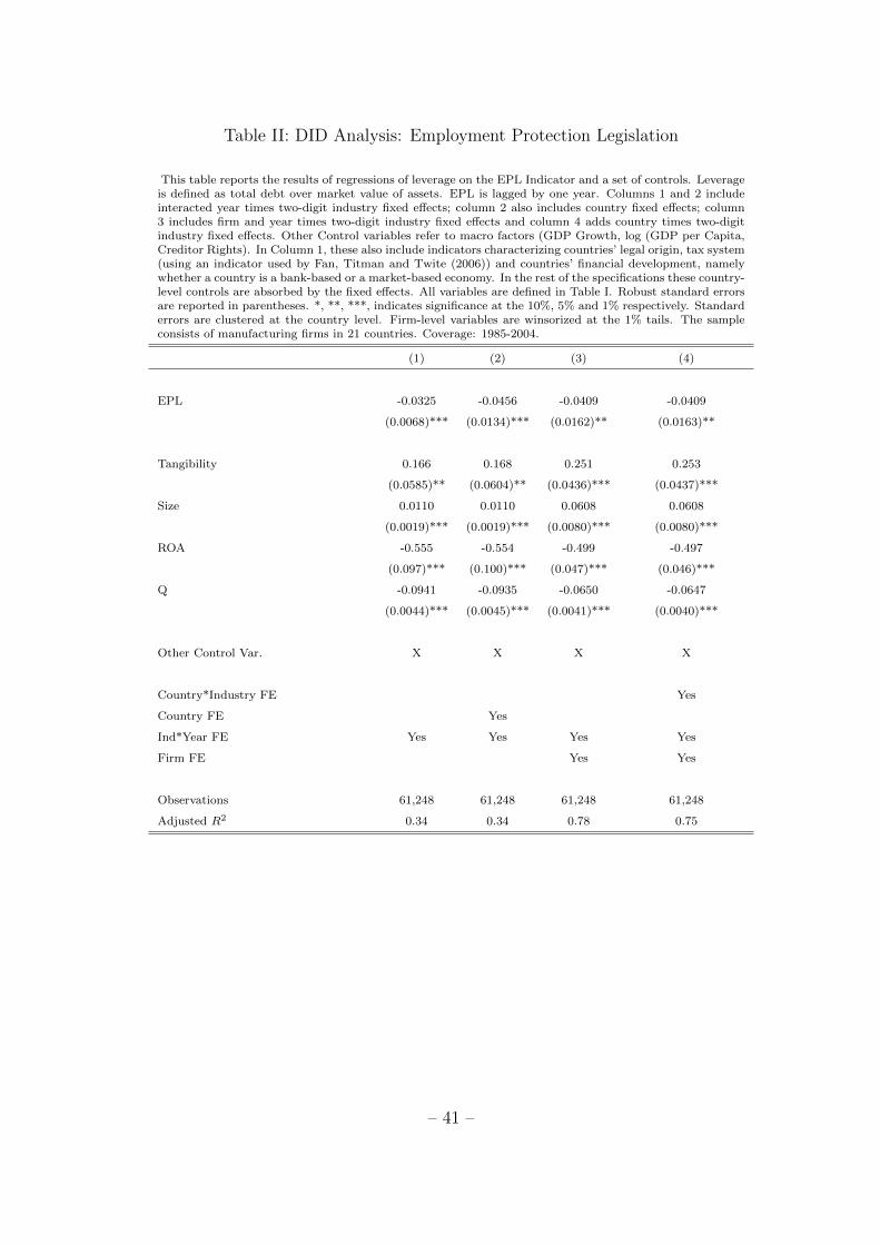
Table II: DID Analysis: Employment Protection Legislation

This table reports the results of regressions of leverage on the EPL Indicator and a set of controls. Leverageis defined as total debt over market value of assets. EPL is lagged by one year. Columns 1 and 2 includeinteracted year times two-digit industry fixed effects; column 2 also includes country fixed effects; column3 includes firm and year times two-digit industry fixed effects and column 4 adds country times two-digitindustry fixed effects. Other Control variables refer to macro factors (GDP Growth, log (GDP per Capita,Creditor Rights). In Column 1, these also include indicators characterizing countries’ legal origin, tax system(using an indicator used by Fan, Titman and Twite (2006)) and countries’ financial development, namelywhether a country is a bank-based or a market-based economy. In the rest of the specifications these country-level controls are absorbed by the fixed effects. All variables are defined in Table I. Robust standard errorsare reported in parentheses. *, **, ***, indicates significance at the 10%, 5% and 1% respectively. Standarderrors are clustered at the country level. Firm-level variables are winsorized at the 1% tails. The sampleconsists of manufacturing firms in 21 countries. Coverage: 1985-2004.

(1) (2) (3) (4)

EPL -0.0325 -0.0456 -0.0409 -0.0409

(0.0068)*** (0.0134)*** (0.0162)** (0.0163)**

Tangibility 0.166 0.168 0.251 0.253

(0.0585)** (0.0604)** (0.0436)*** (0.0437)***

Size 0.0110 0.0110 0.0608 0.0608

(0.0019)*** (0.0019)*** (0.0080)*** (0.0080)***

ROA -0.555 -0.554 -0.499 -0.497

(0.097)*** (0.100)*** (0.047)*** (0.046)***

Q -0.0941 -0.0935 -0.0650 -0.0647

(0.0044)*** (0.0045)*** (0.0041)*** (0.0040)***

Other Control Var. X X X X

Country*Industry FE Yes

Country FE Yes

Ind*Year FE Yes Yes Yes Yes

Firm FE Yes Yes

Observations 61,248 61,248 61,248 61,248

Adjusted R2 0.34 0.34 0.78 0.75

– 41 –

Table III: DID Analysis: Employment Protection Legislation

This table reports the results of regressions of alternate definitions of leverage on the EPL Indicator and a set of controls. Leverage is defined as Total Debt over BookValue of Assets in columns 1-3, as Net Debt (total debt minus cash) over market value of assets in columns 4-6, and as Net Debt over book value of Assets in columns 7-9.EPL and its component are lagged by one year. Columns 1, 4 and 7 include country and interacted year and two-digit industry fixed effects. Columns 2, 5 and 8 includefirm and interacted year and two-digit industry fixed effects and columns 3, 6 and 9 add interacted country and two-digit industry fixed effects. Other Control variablesrefer to macro factors (GDP Growth, log (GDP per Capita, Creditor Rights). All variables are defined in Table I. Robust standard errors are reported in parentheses.*, **, ***, indicates significance at the 10%, 5% and 1% respectively. Standard errors are clustered at the country level. Firm-level variables are winsorized at the 1%tails. The sample consists of manufacturing firms in 21 countries. Coverage: 1985-2004.

Total Debt/Assets Net Debt/Market Value Net Debt/Assets

(1) (2) (3) (4) (5) (6 ) (7) (8) (9)

EPL -0.0273 -0.0261 -0.0265 -0.0493 -0.0478 -0.0285 -0.0281 -0.0283 -0.0481

(0.0094)*** (0.0120)** (0.0122)** (0.0158)*** (0.0167)*** (0.0157)* (0.0116)** (0.0155)* (0.0167)**

Tangibility 0.146 0.129 0.131 0.514 0.653 0.507 0.383 0.504 0.656

(0.0492)*** (0.0240)*** (0.0242)*** (0.1060)*** (0.0697)*** (0.0269)*** (0.3830)*** (0.0283)*** (0.0693)***

Size 0.0120 0.0528 0.0531 0.0183 0.0775 0.0588 0.0124 0.0585 0.0776

(0.0021)*** (0.0066)*** (0.0068)*** (0.0027)*** (0.0084)*** (0.0071)*** (0.0025)*** (0.0069)*** (0.0084)***

ROA -0.374 -0.358 -0.356 -0.503 -0.499 -0.413 -0.387 -0.414 -0.497

(0.0912)*** (0.0362)*** (0.0362)*** (0.1490)*** (0.0482)*** (0.0424)*** (0.1380)*** (0.0427)*** (0.0477)***

Q -0.0098 0.0024 0.0025 -0.0398 0.0028 -0.0091 -0.0423 -0.0092 0.0031

(0.0083) (0.0047) (0.0048) (0.0127)*** (0.0112) (0.0066) (0.0113)*** (0.0065) (0.0113)

Other Control Var. X X X X X X X X X

Country*Industry FE Yes Yes Yes

Country FE Yes Yes Yes

Ind*Year FE Yes Yes Yes Yes Yes Yes Yes Yes Yes

Firm FE Yes Yes Yes Yes Yes Yes

Observations 61,512 61,512 61,512 64,050 64,050 64,050 61,188 61,188 61,188

Adjusted R2 0.14 0.76 0.72 0.19 0.76 0.76 0.19 0.79 0.73

–42

–

Table IV: Cross-sectional Heterogeneity: Labor Intensity and TurnoverThis table reports the results of regressions of cross-sectional heterogeneity. Total debt over market value of assets is regressed on the interaction of EPLwith a proxy of Labor intensity at the industry level and a set of controls. Labor intensity is computed as the median cost of staf over sales for eachindustry defined at the 2-digit level. Turnover is a proxy for employment turnover calculated using data by Davis, Haltiwanger and Schuh (1996). Allcolumns include firm fixed effects. Columns 1 and 5 include firm and year times two-digit industry fixed effects; columns 2 and 6 include firm and countrytimes year fixed effects; Columns 3 and 7 include firm, year times two-digit industry fixed effects and country times year fixed effects and Columns 4 and8 add country times two-digit industry fixed effects to the previous specification. Other Control variables refer to macro factors (GDP Growth, log (GDPper Capita, Creditor Rights). All variables are defined in Table I. Robust standard errors are reported in parentheses. *, **, ***, indicates significanceat the 10%, 5% and 1% respectively. Standard errors are clustered at the country level. Firm-level variables are winsorized at the 1% tails. The sampleconsists of manufacturing firms in 21 countries. Coverage: 1985-2004.

(1) (2) (3) (4) (5) (6) (7) (8)

EPL -0.0160 0.0029

(0.0240) (0.0241)

EPL*Labor Intensity -0.0904 -0.0742 -0.0844 -0.0874

(0.0486)* (0.0397)* (0.0315)*** (0.0369)**

Labor Intensity 0.0450

(0.048)

EPL*Turnover -0.0049 -0.0033 -0.0042 -0.0062

(0.0015)*** (0.0006)*** (0.0009)*** (0.0014)***

Turnover 0.0101

(0.0031)***

Tangibility 0.251 0.229 0.213 0.215 0.251 0.228 0.215 0.212

(0.0435)*** (0.0438)*** (0.0412)*** (0.0419)*** (0.0436)*** (0.0438)*** (0.0412)*** (0.0419)***

Size 0.0608 0.0594 0.0628 0.0632 0.0607 0.0593 0.0632 0.0627

(0.0080)*** (0.0081)*** (0.0081)*** (0.0082)*** (0.0081)*** (0.0082)*** (0.0082)*** (0.0082)***

ROA -0.499 -0.518 -0.512 -0.510 -0.499 -0.518 -0.512 -0.510

(0.0467)*** (0.0506)*** (0.0483)*** (0.0480)*** (0.0467)*** (0.0505)*** (0.0482)*** (0.0480)***

Q -0.0649 -0.0567 -0.0554 -0.0552 -0.0650 -0.0567 -0.0555 -0.0553

(0.0041)*** (0.0031)*** (0.0030)*** (0.0029)*** (0.0041)*** (0.0030)*** (0.0029)*** (0.0029)***

Other Control Var. X X

Firm FE Yes Yes Yes Yes Yes Yes Yes Yes

Ind*Year FE Yes Yes Yes Yes Yes Yes

Country*Year FE Yes Yes Yes Yes Yes Yes

Country*Industry FE Yes Yes

Observations 61,248 61,248 61,248 61,248 61,248 61,248 61,248 61,248

Adjusted R2 0.78 0.79 0.76 0.77 0.78 0.79 0.76 0.77

–43

–

Table V: Cross-sectional Heterogeneity - Liquidation Values

This table reports the results of regressions of cross-sectional heterogeneity. Total debt over assets is regressed onthe interaction of EPL with a proxy for the liquidation value of firms’ assets (L) and a set of controls. The firstproxy L1, is the median tangibility in the industry, L2 is a measure of creditor rights and L3 is the product of thetwo measures (L1*L2). All columns include firm fixed effects. Columns 1, 5 and 7 include also year times two-digitindustry fixed effects. Column 6 controls for year times two-digit industry and country times two-digit industryfixed effects in addition to firm fixed effects. Columns 2 and 8 add year times country fixed effects to the firm fixedeffects, Columns 3 and 9 add country times year and year times two-digit industry fixed effects to the firm fixedeffects and Columns 4 and 10 control for firm, year times two-digit industry, country times year and country timestwo-digit industry fixed effects. Other Control variables refer to macro factors (GDP Growth, log (GDP per Capita,Creditor Rights). All variables are defined in Table I. Robust standard errors are reported in parentheses. *, **,***, indicates significance at the 10%, 5% and 1% respectively. Standard errors are clustered at the country level.Firm-level variables are winsorized at the 1% tails. The sample consists of manufacturing firms in 21 countries.Coverage: 1985-2004.

– 44 –

Table V Continued

(1) (2) (3) (4) (5) (6) (7) (8) (9) (10)

EPL -0.093 -0.105 -0.104 -0.087

(0.0158)*** (0.0214)*** (0.0204)*** (0.0164)***

EPL*L1 0.171 0.088 0.103 0.125

(0.0675)** (0.0548) (0.0588)* (0.0541)**

L1 -0.162

(0.102)

EPL*L2 0.0426 0.0423

(0.0113)*** (0.0111)***

L2 -0.0618 -0.0621

(0.0177)*** (0.0174)***

EPL*L3 0.0980 0.0690 0.0841 0.1000

(0.0259)*** (0.0337)** (0.0252)*** (0.0252)***

L3 -0.116 -0.140 -0.078 -0.022

(0.0397)*** (0.0659)** (0.0809) (0.0843)

Tangibility 0.251 0.229 0.213 0.215 0.247 0.249 0.249 0.229 0.213 0.215

(0.0432)*** (0.0439)*** (0.0412)*** (0.0419)*** (0.0412)*** (0.0413)*** (0.0413)*** (0.0440)*** (0.0410)*** (0.0416)***

Size 0.0608 0.0593 0.0627 0.0632 0.0609 0.0609 0.0609 0.0593 0.0627 0.0633

(0.0080)*** (0.0081)*** (0.0081)*** (0.0082)*** (0.0080)*** (0.0080)*** (0.0079)*** (0.0080)*** (0.0081)*** (0.0081)***

ROA -0.499 -0.518 -0.512 -0.055 -0.498 -0.496 -0.499 -0.518 -0.512 -0.510

(0.0468)*** (0.0505)*** (0.0482)*** (0.0479)*** (0.0465)*** (0.0462)*** (0.0469)*** (0.0505)*** (0.0484)*** (0.0480)***

Q -0.0650 -0.0567 -0.0554 -0.0552 -0.0645 -0.0643 -0.0647 -0.0567 -0.0554 -0.0553

(0.0041)*** (0.0031)*** (0.0030)*** (0.0029)*** (0.0038)*** (0.0037)*** (0.0039)*** (0.0031)*** (0.0030)*** (0.0030)***

Other Control Var. X X X X

Ind.*Country FE Yes Yes Yes

Country*Year FE Yes Yes Yes Yes Yes Yes

Ind.*Year FE Yes Yes Yes Yes Yes Yes Yes Yes

Firm FE Yes Yes Yes Yes Yes Yes Yes Yes Yes Yes

Observations 61,248 61,248 61,248 61,248 61,248 61,248 61,248 61,248 61,248 61,248

Adjusted R2 0.78 0.79 0.76 0.77 0.79 0.76 0.79 0.79 0.76 0.77

–45

–

Table VI: Dynamics of Leverage

This table reports the results of regressions of leverage on the one-year lagged, the contempora-neous and the one-year and two-year forward values of the EPL indicator and a set of controls.Leverage is defined as total debt over Market Value of Assets. Column 1 includes interacted yeartimes two-digit industry fixed effects and country fixed effects; column 2 includes firm and yeartimes two-digit industry fixed effects and column 3 adds country times two-digit industry fixedeffects. Other Control variables refer to macro factors (GDP Growth, log (GDP per Capita,Creditor Rights). All variables are defined in Table I. Robust standard errors are reported inparentheses. *, **, ***, indicates significance at the 10%, 5% and 1% respectively. Standarderrors are clustered at the country level. Firm-level variables are winsorized at the 1% tails. Thesample consists of manufacturing firms in 21 countries. Coverage: 1985-2004.

(1) (2) (3)

EPL(+1) 0.0111 0.0037 0.0050

(0.0106) (0.0109) (0.0110)

EPL(0) -0.0061 -0.0037 -0.0042

(0.0098) (0.0105) (0.0010)

EPL(-1) -0.0203 -0.0148 -0.0139

(0.0052)*** (0.0072)** (0.0073)*

EPL(-2) -0.0272 -0.0290 -0.0298

(0.0068)*** (0.0086)*** (0.0084)***

Other Control Var. X X X

Country*Industry FE Yes

Country FE Yes

Ind*Year FE Yes Yes Yes

Firm FE Yes Yes

Observations 49,171 49,171 49,171

Adjusted R2 0.35 0.80 0.77

– 46 –

Table VII: Growth and Financial Dependence

This table reports the results of regressions of firms’ sales growth on the EPL indicator and a set of controls (Columns 1-3) and onthe interaction of EPL with a proxy for firms’ financial dependence on external capital (constant at the firm level) and a set of controls(Columns 4-7). Column 1 includes country and interacted year and two-digit industry fixed effects; columns 2 and 4 include firm andinteracted year and two-digit industry fixed effects; column 3 adds country times two-digit industry fixed effects. Column 5 controls forfirm and country times year fixed effects. Column 6 adds industry times two-digit industry fixed effects to the previous specification andColumn 7 adds also country times two-digit industry fixed effects to the specification in Column 6. Other Control variables refer to macrofactors (GDP Growth, log (GDP per Capita, Creditor Rights). All variables are defined in Table I. Robust standard errors are reportedin parentheses. *, **, ***, indicates significance at the 10%, 5% and 1% respectively. Standard errors are clustered at the country level.Firm-level variables are winsorized at the 1% tails. The sample consists of manufacturing firms in 21 countries. Coverage: 1985-2004.

Growth of Sales Growth of Sales

(1) (2) (3) (4) (5) (6) (7)

EPL -0.0037 -0.0388 -0.0386 -0.0429

(0.018)** (0.023)* (0.023)* (0.0224)*

EPL*Financial -0.00575 -0.00399 -0.00495 -0.00442

Dependence (0.00156)*** (0.00121)*** (0.0014)*** (0.0010)***

ROA 0.334 0.639 0.638 0.636 0.6545 0.6256 0.6253

(0.048)*** (0.043)*** (0.044)*** (0.0452)*** (0.0369)*** (0.03797)*** (0.03807)***

Q 0.044 0.024 0.024 0.0251 0.0292 0.0287 0.0285

(0.006)*** (0.007)*** (0.007)*** (0.00706)*** (0.0061)*** (0.0062)*** (0.0063)***

Other Control Var. X X X X

Firm FE Yes Yes Yes Yes Yes Yes

Country FE Yes

Ind*Year FE Yes Yes Yes Yes Yes Yes

Country*Year FE Yes Yes Yes

Country*Industry FE Yes Yes

Observations 66,456 66,456 66,456 64,973 64,973 64,973 64,973

Adjusted R2 0.14 0.34 0.25 0.34 0.27 0.28 0.28

–47

–

Table VIII: Capital Expenditure and Financial Dependence

This table reports the results of regressions of firms’ investment measured as capital expenditures over assets on the EPL indicator anda set of controls (Columns 1-3) and on the interaction of EPL with a proxy for firms’ financial dependence on external capital (constantat the firm level) and a set of controls (Columns 4-7). Column 1 includes country and interacted year and two-digit industry fixed effects;columns 2 and 4 include firm and interacted year and two-digit industry fixed effects; column 3 adds country times two-digit industryfixed effects. Column 5 controls for firm and country times year fixed effects. Column 6 adds industry times two-digit industry fixedeffects to the previous specification and Column 7 adds also country times two-digit industry fixed effects to the specification in Column 6.Other Control variables refer to macro factors (GDP Growth, log (GDP per Capita, Creditor Rights). All variables are defined in Table I.Robust standard errors are reported in parentheses. *, **, ***, indicates significance at the 10%, 5% and 1% respectively. Standard errorsare clustered at the country level. Firm-level variables are winsorized at the 1% tails. The sample consists of manufacturing firms in 21countries. Coverage: 1985-2004.

Capex/Assets Capex/Assets

(1) (2) (3) (4) (5) (6) (7)

EPL 0.0002 -0.0009 -0.0008 -0.00183

(0.002) (0.003) (0.003) (0.00310)

EPL*Financial -0.00115 -0.00105 -0.00115 -0.00116

Dependence (0.0003)*** (0.00027)*** (0.00029)*** (0.00028)***

ROA 0.044 0.028 0.028 0.0279 0.0258 0.0243 0.0242

(0.004)*** (0.004)*** (0.004)*** (0.0037)*** (0.0029)*** (0.0031)*** (0.0031)***

Q 0.004 0.003 0.004 0.00335 0.0043 0.0042 0.0042

(0.001)*** (0.001)*** (0.001)*** (0.0006)*** (0.00047)*** (0.00049)*** (0.0005)***

Other Control Var. X X X X

Firm FE Yes Yes Yes Yes Yes Yes

Country FE Yes

Ind*Year FE Yes Yes Yes Yes Yes Yes

Country*Year FE Yes Yes Yes

Country*Industry FE Yes Yes

Observations 56,723 56,723 56,723 56,641 56,641 56,641 56,641

Adjusted R2 0.15 0.55 0.48 0.55 0.49 0.49 0.49

–48

–

Table IX: Firms’ Profitability and Cost of Labor

This table reports the results of regressions of net firms’ profitability (columns 1-3) and labor costs (columns 4-6) onthe EPL indicator and a set of controls. Columns 1 and 4 include country and interacted year and two-digit industryfixed effects; columns 2 and 5 include firm and interacted year and two-digit industry fixed effects; columns 3 and6 add country times two-digit industry fixed effects. Other Control variables refer to macro factors (GDP Growth,log (GDP per Capita, Creditor Rights). All variables are defined in Table I. Robust standard errors are reported inparentheses. *, **, ***, indicates significance at the 10%, 5% and 1% respectively. Standard errors are clustered atthe country level. Firm-level variables are winsorized at the 1% tails. The sample consists of manufacturing firmsin 21 countries. Coverage: 1985-2004.

ROA Cost of Staff/Assets

(1) (2) (3) (4) (5) (6)

EPL -0.0091 -0.0140 -0.0147 0.0525 0.0281 0.0277

(0.0060) (0.0059)** (0.0057)*** (0.0168)*** (0.0132)** (0.0130)**

Tangibility 0.027 -0.099 -0.099 0.123 0.125 0.125

(0.017) (0.011)*** (0.011)*** (0.036)*** (0.033)*** (0.032)***

Size 0.0100 0.0156 0.0157 -0.0229 -0.0608 -0.0617

(0.0021)*** (0.0037) (0.0037)*** (0.0013)*** (0.0044) (0.0044)***

ROA 0.0219 -0.1030 -0.1040

(0.0209) (0.0100) (0.0102)***

Q 0.0262 0.0307 0.0305 -0.0164 -0.0034 -0.0036

(0.0038)*** (0.0041)*** (0.0041)*** (0.0030)*** (0.0018)* (0.0018)**

Other Control Var. X X X X X X

Country*Industry FE Yes Yes

Country FE Yes Yes

Ind*Year FE Yes Yes Yes Yes Yes Yes

Firm FE Yes Yes Yes Yes

Observations 64,732 64,732 64,732 13,461 13,461 13,461

Adjusted R2 0.16 0.61 0.55 0.38 0.90 0.88

– 49 –

Figure 1: Timeline

Entrepreneur set up a project: • Raising external capital F . • Hiring n workers.

• Cash flow C1 is realized • Project can be liquidated for

L .

0 1

t

1.5 2

• Cash flow C2 is realized

• Entrepreneur and workers learn productivity of incumbent workers.

• Bargaining between entrepreneurs and incumbent workers.

• Firing and hiring decision by the entrepreneur.

–50

–

Figure 2: EPL

01

23

40

12

34

01

23

4

1985 1990 1995 2000 2005 1985 1990 1995 2000 2005 1985 1990 1995 2000 2005 1985 1990 1995 2000 2005 1985 1990 1995 2000 2005 1985 1990 1995 2000 2005 1985 1990 1995 2000 2005

AUSTRALIA AUSTRIA BELGIUM CANADA DENMARK FINLAND FRANCE

GERMANY GREECE IRELAND ITALY JAPAN NETHERLANDS NEW ZEALAND

NORWAY PORTUGAL SPAIN SWEDEN SWITZERLAND UNITED KINGDOM UNITED STATES

Em

ploy

men

t Pro

tect

ion

Legi

slat

ion

(EP

L)

yearGraphs by country

�

–51

–

Figure 3: Differential Effect of EPL on Leverage for different degrees of Creditor Protection

FR

US, CH, PT, GR

IE CA

SEFI

NO, IT, BE

ES

JP

NL, DE, DK, AT, AU

NZ, UK

-0.12

-0.1

-0.08

-0.06

-0.04

-0.02

0

0.02

0.04

0.06

0.08

0 0.5 1 1.5 2 2.5 3 3.5 4 4.5dD/d

EPL

Creditor Rights

Figure 2: Differential Effect of EPL on Leverage for different degrees of Creditor Protection

–52

–