labor demand response to labor supply incentives: evidence...

Labor demand response to labor supply incentives: Evidencefrom the German Mini-Job reform

Online Appendix

Gabriela Galassi

European University Institute

January 15, 2018

Abstract

This Online Appendix contains additional information for the paper “Labor demand responseto labor supply incentives: Evidence from the German Mini-Job reform”. Appendix A providesadditional tables, and Appendix B, figures that complement the analysis. Appendix C presentsdetails on the data. Finally, Appendix D comprises derivations corresponding to the theoreticalframework in the paper.

A Additional Tables

Table A.1: Social Security average tax rates and monthly gross earnings limitsRegular employment Mini-jobs Midi-jobs

Worker rate Employer rate Earnings Worker rate Employer rate Earnings Worker rate Employer rate

1999-30 Mar 2003 21% 21% e0-e325 0% 22% -1 Apr 2003-30 Jun 2006 21% 21% e0-e400 0% 25% e401-e800 4.1%-21% 21%1 Jul 2006-31 Dec 2007 19.5% 19.5% e0-e400 0% 30% e401-e800 4.1%-19.5% 19.5%

Note: Only for the period 1999-2007. SSC rates are in terms of gross earnings, income tax rates (to which mini-jobs are

exempted) are not included.

Table A.2: Hours of work by type of worker, 2005

Type of job Hours a week Hourly (net) wage

Regular part-time 13 19(5.68) (21.20)

Regular full-time 41 9(9.50) (4.16)

Mini-job (main) 14 10(12.00) (25.59)

Mini-job (secondary) 40 9(13.97) (6.59)

Midi-job (main) 26 8(13.86) (16.41)

Midi-job (secondary) 36 15(16.96) (12.38)

Total 34 10(15.21) (11.94)

Note: Data from G-SOEP. Standard errors in parenthesis. Hours worked and hourly net earnings for valid responses.

Workers 17-65 years old.

1

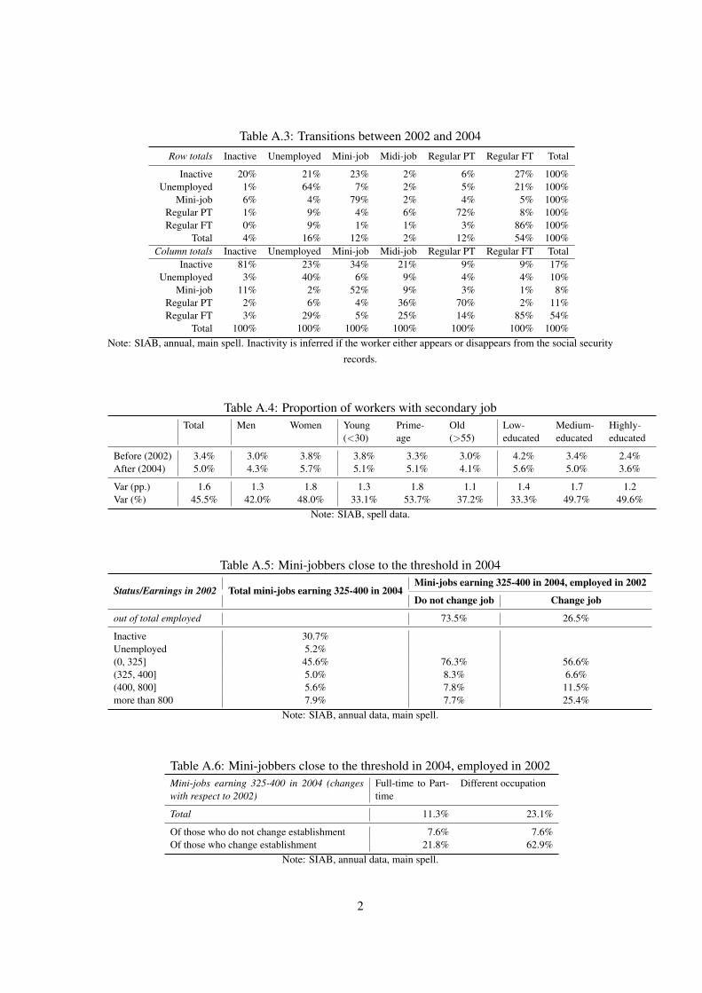
Table A.3: Transitions between 2002 and 2004Row totals Inactive Unemployed Mini-job Midi-job Regular PT Regular FT Total

Inactive 20% 21% 23% 2% 6% 27% 100%Unemployed 1% 64% 7% 2% 5% 21% 100%

Mini-job 6% 4% 79% 2% 4% 5% 100%Regular PT 1% 9% 4% 6% 72% 8% 100%Regular FT 0% 9% 1% 1% 3% 86% 100%

Total 4% 16% 12% 2% 12% 54% 100%Column totals Inactive Unemployed Mini-job Midi-job Regular PT Regular FT Total

Inactive 81% 23% 34% 21% 9% 9% 17%Unemployed 3% 40% 6% 9% 4% 4% 10%

Mini-job 11% 2% 52% 9% 3% 1% 8%Regular PT 2% 6% 4% 36% 70% 2% 11%Regular FT 3% 29% 5% 25% 14% 85% 54%

Total 100% 100% 100% 100% 100% 100% 100%Note: SIAB, annual, main spell. Inactivity is inferred if the worker either appears or disappears from the social security

records.

Table A.4: Proportion of workers with secondary jobTotal Men Women Young

(<30)Prime-age

Old(>55)

Low-educated

Medium-educated

Highly-educated

Before (2002) 3.4% 3.0% 3.8% 3.8% 3.3% 3.0% 4.2% 3.4% 2.4%After (2004) 5.0% 4.3% 5.7% 5.1% 5.1% 4.1% 5.6% 5.0% 3.6%

Var (pp.) 1.6 1.3 1.8 1.3 1.8 1.1 1.4 1.7 1.2Var (%) 45.5% 42.0% 48.0% 33.1% 53.7% 37.2% 33.3% 49.7% 49.6%

Note: SIAB, spell data.

Table A.5: Mini-jobbers close to the threshold in 2004

Status/Earnings in 2002 Total mini-jobs earning 325-400 in 2004Mini-jobs earning 325-400 in 2004, employed in 2002

Do not change job Change job

out of total employed 73.5% 26.5%

Inactive 30.7%Unemployed 5.2%(0, 325] 45.6% 76.3% 56.6%(325, 400] 5.0% 8.3% 6.6%(400, 800] 5.6% 7.8% 11.5%more than 800 7.9% 7.7% 25.4%

Note: SIAB, annual data, main spell.

Table A.6: Mini-jobbers close to the threshold in 2004, employed in 2002Mini-jobs earning 325-400 in 2004 (changeswith respect to 2002)

Full-time to Part-time

Different occupation

Total 11.3% 23.1%

Of those who do not change establishment 7.6% 7.6%Of those who change establishment 21.8% 62.9%

Note: SIAB, annual data, main spell.

2

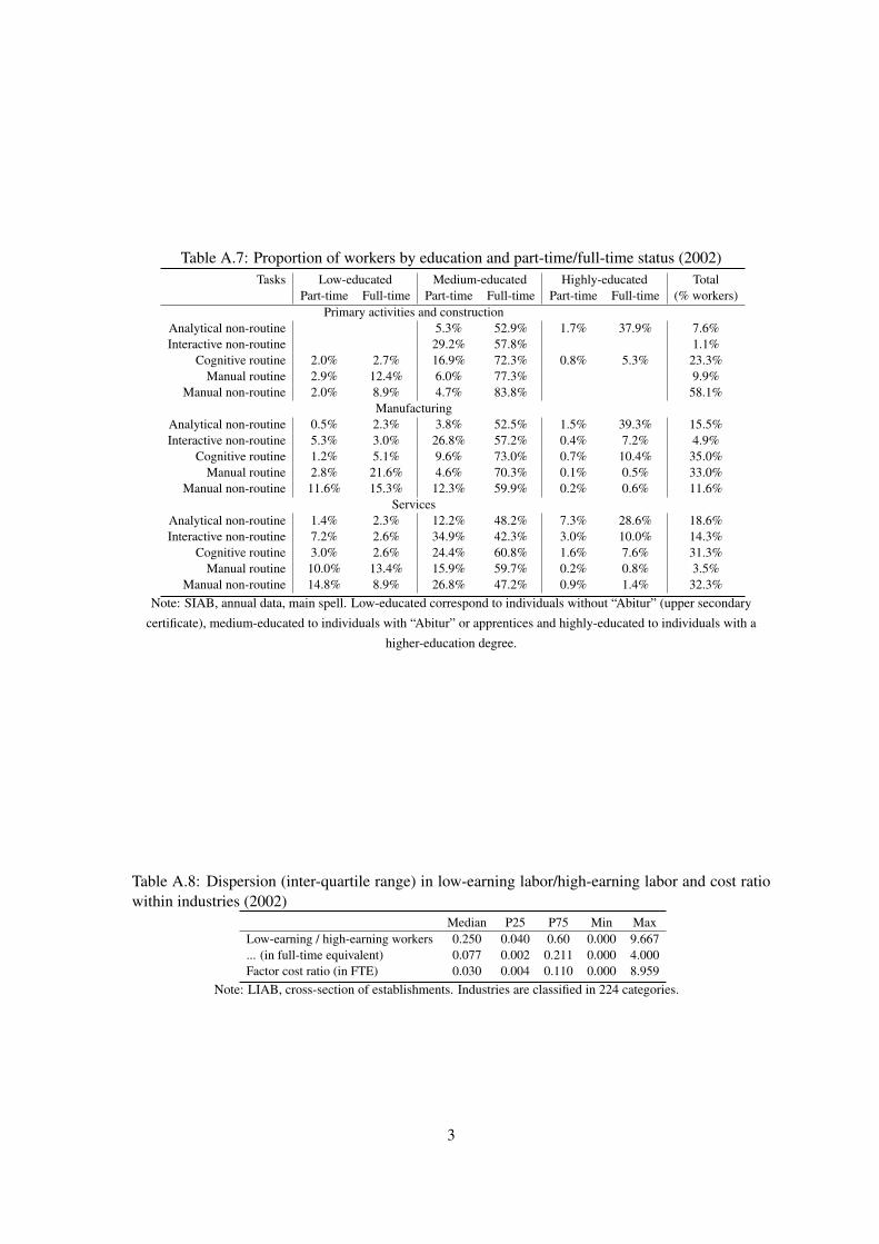
Table A.7: Proportion of workers by education and part-time/full-time status (2002)Tasks Low-educated Medium-educated Highly-educated Total

Part-time Full-time Part-time Full-time Part-time Full-time (% workers)Primary activities and construction

Analytical non-routine 5.3% 52.9% 1.7% 37.9% 7.6%Interactive non-routine 29.2% 57.8% 1.1%

Cognitive routine 2.0% 2.7% 16.9% 72.3% 0.8% 5.3% 23.3%Manual routine 2.9% 12.4% 6.0% 77.3% 9.9%

Manual non-routine 2.0% 8.9% 4.7% 83.8% 58.1%Manufacturing

Analytical non-routine 0.5% 2.3% 3.8% 52.5% 1.5% 39.3% 15.5%Interactive non-routine 5.3% 3.0% 26.8% 57.2% 0.4% 7.2% 4.9%

Cognitive routine 1.2% 5.1% 9.6% 73.0% 0.7% 10.4% 35.0%Manual routine 2.8% 21.6% 4.6% 70.3% 0.1% 0.5% 33.0%

Manual non-routine 11.6% 15.3% 12.3% 59.9% 0.2% 0.6% 11.6%Services

Analytical non-routine 1.4% 2.3% 12.2% 48.2% 7.3% 28.6% 18.6%Interactive non-routine 7.2% 2.6% 34.9% 42.3% 3.0% 10.0% 14.3%

Cognitive routine 3.0% 2.6% 24.4% 60.8% 1.6% 7.6% 31.3%Manual routine 10.0% 13.4% 15.9% 59.7% 0.2% 0.8% 3.5%

Manual non-routine 14.8% 8.9% 26.8% 47.2% 0.9% 1.4% 32.3%Note: SIAB, annual data, main spell. Low-educated correspond to individuals without “Abitur” (upper secondary

certificate), medium-educated to individuals with “Abitur” or apprentices and highly-educated to individuals with a

higher-education degree.

Table A.8: Dispersion (inter-quartile range) in low-earning labor/high-earning labor and cost ratiowithin industries (2002)

Median P25 P75 Min MaxLow-earning / high-earning workers 0.250 0.040 0.60 0.000 9.667... (in full-time equivalent) 0.077 0.002 0.211 0.000 4.000Factor cost ratio (in FTE) 0.030 0.004 0.110 0.000 8.959

Note: LIAB, cross-section of establishments. Industries are classified in 224 categories.

3

Table A.9: Characteristics of establishments in 2002, cross-section and panel (2000-2007),weighted/unweighted

Cross-section PanelUnweighted Weighted Unweighted Weighted

Establishment age 15.2 13.2 14.5 14.2Establishment size (n. of workers) 164.4 15.6 161.6 18.5Proportion of workers below 2003 MJ threshold 15.5% 27.8% 16.0% 29.2%Proportion of workers below 2003 MidiJ threshold 21.4% 37.7% 21.4% 37.6%Proportion of marginal part-time workers 9.9% 18.6% 10.5% 20.4%Proportion of part-time workers 23.2% 31.2% 23.0% 32.1%Proportion of temporary workers 5.7% 3.0% 5.3% 3.1%Proportion of low-educated workers 13.8% 13.0% 12.6% 11.5%Proportion of medium-educated workers 62.7% 58.6% 65.9% 58.0%Proportion of highly-educated workers 7.5% 3.7% 7.5% 4.3%Proportion of female workers 46.2% 55.1% 46.4% 56.7%Proportion of working proprietors 8.4% 20.4% 9.5% 19.8%Proportion of trainees/apprentices 5.1% 4.6% 5.0% 4.7%Median daily gross wage 61.2 44.3 58.3 45.0Median daily wage full-time 72.6 59.7 68.9 61.5Median daily wage part-time 32.8 20.0 32.8 19.6Median daily wage low-earnings 9.2 9.1 8.9 9.2Median daily wage high-earnings 68.0 56.8 65.1 58.8Monthly per capita labor cost 1,865.2 1,353.1 1,748.3 1,396.3Total monthly labor cost 479,785 33,551 478,390 43,405Investment (million) 2.146 0.116 1.877 0.118Sales (million) 37.483 2.493 29.975 2.967Exports/revenues 10.9% 4.2% 10.5% 4.1%Hirings/employment 0.19 0.21 0.17 0.19Separations/employment 0.60 0.32 0.25 0.26Work council 40.4% 10.2% 38.7% 9.9%Collective agreement 57.8% 43.5% 57.3% 44.6%Agriculture, primary 4.3% 3.7% 4.4% 4.0%Manufacturing 26.1% 11.9% 28.6% 12.9%Construction 8.9% 10.8% 9.7% 10.5%Retail, repair 13.0% 22.1% 12.5% 21.5%Transport, communication 3.6% 5.1% 3.1% 4.8%Financial intermediation 3.0% 2.3% 2.6% 2.3%Services for businesses 11.4% 15.3% 8.3% 15.7%Other services 19.4% 23.5% 18.3% 23.2%Public administration 10.4% 5.3% 12.5% 5.0%Proportion of workers in analytical non-routine tasks 14.8% 10.6% 13.5% 11.1%Proportion of workers in interactive non-routine tasks 8.9% 12.0% 8.7% 11.3%Proportion of workers in cognitive routine tasks 31.5% 34.6% 31.4% 35.9%Proportion of workers in manual routine tasks 12.8% 8.2% 14.5% 8.7%Proportion of workers in manual non-routine tasks 28.5% 31.5% 28.2% 30.1%New firm (Estab. Panel) 2.5% 9.2%Firm death 1.6% 2.9%Observations 14,591 3,770

4

Table A.10: Characteristics of establishments by proportion of low-earning workers (quintiles),2002

Q1 Q2 Q3 Q4 Q5Proportion of workers below 2003 MJ threshold 0% 6.2% 24.3% 46.3% 83.2%Proportion of workers below 2003 MidiJ threshold 11.8% 11.2% 34.0% 54.6% 85.7%Establishment age 14.7 18.5 14.7 13.0 11.8Establishment size (n. workers) 9.1 97.2 14.6 9.2 6.2Establishment size (full-time equivalent) 8.4 87.3 11.5 6.3 3.3Proportion of part-time workers 13.0% 17.7% 28.7% 42.7% 67.9%Proportion of low-educated workers 9.2% 13.2% 12.2% 13.7% 11.6%Proportion of medium-educated workers 65.6% 66.2% 60.2% 51.8% 43.2%Proportion of highly-educated workers 5.6% 9.1% 4.5% 2.9% 0.4%Vacancies/employment 3.0% 1.6% 1.2% 1.6% 0.7%Median daily gross wage 59.0 72.8 50.8 31.2 9.9Median daily gross wage (growth) 19.0% 2.9% 9.6% 22.6% -7.2%Median daily gross wage of full-time workers 64.5 80.2 63.8 56.2 38.8Median daily gross wage of full-time workers (growth) 4.2% 2.5% 0.7% 5.6% 4.2%Median daily gross wage of part-time workers 46.2 33.9 16.4 12.4 9.0Median daily gross wage of part-time workers (growth) 16.6% 22.0% 10.3% 7.1% 14.5%Per capita monthly labor cost 1,548 2,148 1,551 1,068 783Monthly wage bill 23,581 263,505 28,967 11,041 4,878Inequality (P75/P25) full-time workers 1.38 1.39 1.67 2.30 1.61Hirings/employment 0.14 0.18 0.19 0.25 0.23Separations/employment 0.30 0.19 0.20 0.26 0.33Investment (million) 0.057 0.777 0.057 0.033 0.037Sales (million) 1.627 21.291 1.565 0.566 0.448Exports/revenues 4.2% 11.8% 2.5% 3.4% 3.1%Work council 11.2% 37.3% 7.6% 4.5% 1.4%Collective agreement 47.3% 58.8% 49.6% 40.5% 28.6%Agriculture, primary 7.9% 1.7% 2.0% 2.5% 3.0%Manufacturing 13.0% 25.3% 10.5% 13.6% 8.9%Construction 16.0% 12.9% 12.5% 3.2% 3.6%Retail, repair 19.4% 12.8% 24.1% 23.6% 24.2%Transport, communication 6.6% 5.9% 2.5% 2.4% 6.6%Financial intermediation 3.5% 2.6% 1.9% 1.3% 1.8%Services for businesses 8.5% 12.3% 18.3% 26.2% 16.4%Other services 19.1% 18.5% 26.0% 24.8% 27.2%Public sector 5.9% 8.0% 2.3% 2.5% 8.4%Workers in analytical non-routine tasks 15.6% 15.2% 9.0% 8.1% 7.2%Workers in interactive non-routine tasks 9.0% 11.0% 10.2% 12.4% 16.3%Workers in cognitive routine tasks 32.1% 33.2% 41.2% 38.3% 34.0%Workers in manual routine tasks 12.2% 10.5% 8.2% 7.3% 3.9%Workers in manual non-routine tasks 29.8% 27.8% 28.8% 28.5% 35.4%Observations 1,041 1,288 852 306 283

Note: Panel 2000-2002. Establishments classified according to the (weighted) quintile of the proportion of low-earning

workers.

5

Table A.11: Empirical test: variations in employment by typeCoexistence of scale and substitution effect (0 < σ < η)

Intensive (s1H) Non-intensive (s1L) Diff. (Int. - Non Int.)N1k ↑ (scale) ↑ (substitution) >=< 0N2k ↑↑ ↑ > 0

N1k +N2k ↑↑ ↑ > 0Only substitution effect (σ > η)

Intensive (s1H) Non-intensive (s1L) Diff. (Int. - Non Int.)N1k ↑ ↑↑ < 0N2k ↓↓ ↓ < 0

N1k +N2k ↓↑ ↑↓ >=< 0Only scale effect (σ = 0)

Intensive (s1H) Non-intensive (s1L) Diff. (Int. - Non Int.)N1k ↑↑ ↑ > 0N2k ↑↑ ↑ > 0

N1k +N2k ↑↑ ↑ > 0Note: The direction and magnitudes of the effects correspond to the expression:

dlnN1kdlnw1

=−[s1kη +(1− s1k)σ ]dlnN2kdlnw1

=−[s1kη− s1kσ ]

6

Table A.12: Estimates of the differences-in-differences coefficients1999-2002 2002-2004 2002-2007

β1999 β2000 β2001 βPost

Total employment -0.063 -0.289 -0.344 0.463 0.873*(0.8148) (0.5562) (0.3313) (0.2577) (0.3632)

Total full-time equivalent employment 0.651 0.136 -0.134 0.763*** 1.370***(0.7153) (0.4749) (0.2692) (0.2238) (0.2912)

Low-earning workers (growth) -0.127 -0.488 -0.447* -0.413**(0.3555) (0.3351) (0.2149) (0.1558)

Higher-earning workers (growth) 0.170 0.067 0.300 0.103(0.1694) (0.1449) (0.1596) (0.1093)

Part-time workers -0.178 0.105 -0.069 -0.723*** -0.852***(0.3878) (0.2911) (0.1825) (0.1608) (0.1961)

Full-time workers 0.586 -0.030 -0.118 1.182*** 1.873***(0.5732) (0.3638) (0.2463) (0.2069) (0.2711)

Proportion of low-educated workers -0.014 -0.014 -0.004 -0.038* -0.042*(0.0312) (0.0164) (0.0154) (0.0187) (0.0204)

Number of medium-educated workers 0.794 0.236 0.052 0.578** 0.963***(0.6540) (0.4179) (0.2219) (0.1865) (0.2453)

Median gross daily wage (growth) 0.175 0.235 0.497*** 0.324***(0.1756) (0.1588) (0.1144) (0.1084)

Median gross daily wage full-time (growth) 0.057 0.002 0.134 0.093(0.1056) (0.0570) (0.0730) (0.0482)

Median gross daily wage of part-time (growth) 0.103 -0.151 0.451*** 0.054(0.1408) (0.0982) (0.1279) (0.2144)

Total investment (euros) -61,213 -45,864 -61,997 9,235 6,408(40870.5) (34493.8) (43756.7) (32644.1) (32603.5)

Vacancies (ln) 0.092 0.411 0.395 0.269(0.2960) (0.3240) (0.2017) (0.1817)

Hirings of workers earning 800-1200 0.024 -0.045 0.069 0.117***(0.0598) (0.0525) (0.0402) (0.0340)

Hirings of workers earning 1600-2000 0.052 -0.107 0.163** 0.189***(0.0970) (0.0919) (0.0541) (0.0571)

Wage of part-time hiring 7.121 0.124 1.692 4.524*(3.7899) (3.1635) (2.2834) (2.2909)

Wage of full-time hiring -9.124 5.391 -0.587 -10.362(8.3273) (7.8964) (5.5420) (6.6588)

Frequency of wage upgrade 0.148* 0.164* 0.098 0.069(0.0673) (0.0705) (0.0524) (0.0440)

Frequency of wage downgrade -0.037 -0.031 -0.062 -0.098(0.0734) (0.0496) (0.0690) (0.0572)

Proportion of workers in analytical non-routine tasks 0.019 0.023 0.010 0.011 0.016(0.0250) (0.0176) (0.0121) (0.0089) (0.0096)

Proportion of workers in interactive non-routine tasks 0.009 0.002 -0.005 -0.006 -0.006(0.0165) (0.0102) (0.0090) (0.0086) (0.0100)

Note: Estimates from equation (4). Different rows correspond to different outcomes. Columns 1-3 shows estimates of β

over the 1999-2002 period. Column 4 shows estimates of β for the 2002-2004 period (short-run), and column 5, for

2002-2007 (medium-run), both using an indicator variable Post that takes the value 1 for 2003 on. Standard errors in

parentheses. * p<0.05, ** p<0.01, *** p<0.001. Growth rates of low-earning and high-earning workers are estimated

on the subsample of establishments with both types of workers (quintiles 2 to 4 of intensity in low-earning workers).

7

Table A.13: Estimates of the differences-in-differences coefficients, heterogeneous effectsEmployment FTE employment Part-time Full-time Low-educated (proportion) Medium-educated

IndustryIntLE 1.65* 1.68** 0.02 1.64** -0.09 1.19*(baseline: Primaries, construction) (0.688) (0.583) (0.434) (0.522) (0.110) (0.480)IntLE ×Manufacturing 0.88 1.65 -1.16 2.43 0.15 1.31

(1.912) (1.676) (0.968) (1.610) (0.113) (1.394)IntLE × Services -0.39 -0.25 -0.41 0.03 0.04 0.19

(0.878) (0.726) (0.521) (0.655) (0.112) (0.612)

R2 0.11 0.12 0.06 0.12 0.07 0.09Establishment age

IntLE 0.90 0.67 0.22 0.54 -0.02 0.91(baseline: 0-9 y.o.) (0.730) (0.588) (0.370) (0.528) (0.022) (0.515)IntLE × 10-19 y.o. 0.70 1.45 -0.56 1.79 -0.05 1.33

(1.237) (1.015) (0.514) (0.956) (0.059) (0.869)IntLE × 20-29 y.o. 0.72 1.54 -1.68** 2.55** -0.02 0.47

(1.139) (0.972) (0.564) (0.908) (0.052) (0.751)

R2 0.11 0.12 0.06 0.12 0.07 0.09Establishment size

IntLE 0.35 0.34 -0.25 0.44 -0.05 0.56(baseline: 1-5 work.) (0.410) (0.359) (0.196) (0.325) (0.028) (0.317)IntLE × 6-20 work. 1.03 0.55 1.13 -0.09 0.03 0.72

(0.839) (0.665) (0.610) (0.618) (0.031) (0.613)IntLE × 21-200 work. 5.23 7.18* 2.22 6.04 0.09 7.05*

(5.217) (3.483) (3.381) (3.115) (0.051) (2.980)IntLE × 201 or more work. 20.21 41.93 -4.72 48.29** 0.07 24.24

(37.146) (23.775) (31.229) (17.603) (0.039) (15.611)

R2 0.11 0.13 0.09 0.14 0.07 0.09Collective agreement (industry or company level)

IntLE 0.73 0.83 -0.21 0.90* -0.04 1.07**(baseline: No agreement) (0.515) (0.436) (0.258) (0.406) (0.025) (0.361)IntLE × Agreement 1.66 1.92* -0.51 2.38** -0.00 0.91

(0.994) (0.784) (0.523) (0.730) (0.051) (0.619)

R2 0.11 0.12 0.06 0.12 0.07 0.09

Note: Estimates from equation (6.5). Different columns correspond to different outcomes, and different panels

correspond to different variables in the heterogeneity analysis. Standard errors in parentheses. * p<0.05, ** p<0.01,

*** p<0.001. Controlling for industry specific (224 categories) quadratic trends.

8

Table A.14: Estimates for βt for total employment - Specific trendsBenchmark Quadratic trend Quadratic trend Linear trend Controls for

quintiles LE share industry firm-specific (FD) pre-trend1999 -0.109 2.819 0.114 -0.121

(0.8734) (2.1425) (0.7532) (0.8745)2000 -0.409 1.229 -0.522 -0.496 -0.411

(0.5696) (1.2483) (0.5381) (0.5147) (0.5692)2001 -0.472 0.182 -0.491 -0.395 -0.469

(0.3362) (0.6493) (0.3398) (0.6099) (0.3362)2002 baseline2003 0.276 -0.049 0.406 -0.058 0.286

(0.2140) (0.4726) (0.2302) (0.3990) (0.2127)2004 0.666 0.304 0.914** 0.070 0.677*

(0.3400) (0.9055) (0.3478) (0.4347) (0.3398)2005 1.246** 1.120 1.569*** 0.262 1.243**

(0.4326) (1.2710) (0.4602) (0.4419) (0.4327)2006 1.325** 1.748 1.767*** -0.220 1.297**

(0.4755) (1.6606) (0.5366) (0.4028) (0.4822)2007 0.891 2.147 1.374* -0.760 0.867

(0.5657) (2.2076) (0.6290) (0.4124) (0.5692)LE industry (other commuting zones) -7.263

(7.0162)LE commuting zone (other industries) -0.480

(1.9197)

Note: Standard errors in parentheses. * p<0.05, ** p<0.01, *** p<0.001.

Table A.15: Estimates for βt for total full-time equivalent employment - Specific trendsBenchmark Quadratic trend Quadratic trend Linear trend Controls for

quintiles LE share industry firm-specific (FD) pre-trend1999 0.506 2.145 0.799 0.489

(0.7722) (1.8038) (0.6559) (0.7739)2000 -0.077 0.824 -0.141 -0.537 -0.081

(0.4881) (1.0433) (0.4710) (0.4366) (0.4884)2001 -0.264 0.065 -0.241 -0.416 -0.267

(0.2752) (0.5404) (0.2748) (0.4817) (0.2756)2002 baseline2003 0.434* 0.344 0.529** 0.329 0.441*

(0.1849) (0.3896) (0.1941) (0.3138) (0.1836)2004 1.087*** 1.105 1.285*** 0.566 1.091***

(0.2917) (0.7457) (0.2945) (0.3486) (0.2900)2005 1.783*** 2.105* 2.056*** 0.588 1.776***

(0.3324) (0.9797) (0.3512) (0.3514) (0.3333)2006 1.903*** 2.748* 2.307*** 0.055 1.885***

(0.3796) (1.2435) (0.4080) (0.3236) (0.3886)2007 1.678*** 3.251* 2.159*** -0.338 1.659***


(6.4675)LE commuting zone (other industries) 0.376

(1.6108)


9

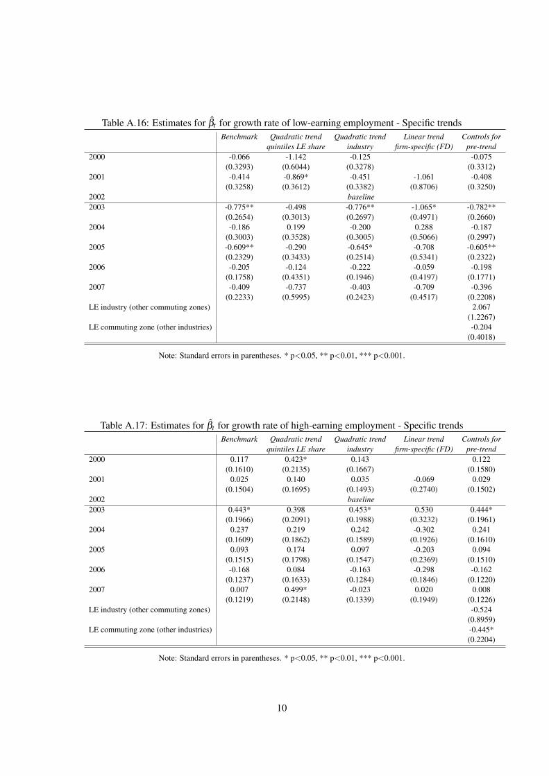
Table A.16: Estimates for βt for growth rate of low-earning employment - Specific trendsBenchmark Quadratic trend Quadratic trend Linear trend Controls for

quintiles LE share industry firm-specific (FD) pre-trend2000 -0.066 -1.142 -0.125 -0.075

(0.3293) (0.6044) (0.3278) (0.3312)2001 -0.414 -0.869* -0.451 -1.061 -0.408

(0.3258) (0.3612) (0.3382) (0.8706) (0.3250)2002 baseline2003 -0.775** -0.498 -0.776** -1.065* -0.782**

(0.2654) (0.3013) (0.2697) (0.4971) (0.2660)2004 -0.186 0.199 -0.200 0.288 -0.187

(0.3003) (0.3528) (0.3005) (0.5066) (0.2997)2005 -0.609** -0.290 -0.645* -0.708 -0.605**

(0.2329) (0.3433) (0.2514) (0.5341) (0.2322)2006 -0.205 -0.124 -0.222 -0.059 -0.198

(0.1758) (0.4351) (0.1946) (0.4197) (0.1771)2007 -0.409 -0.737 -0.403 -0.709 -0.396

(0.2233) (0.5995) (0.2423) (0.4517) (0.2208)LE industry (other commuting zones) 2.067


(0.4018)


Table A.17: Estimates for βt for growth rate of high-earning employment - Specific trendsBenchmark Quadratic trend Quadratic trend Linear trend Controls for

quintiles LE share industry firm-specific (FD) pre-trend2000 0.117 0.423* 0.143 0.122

(0.1610) (0.2135) (0.1667) (0.1580)2001 0.025 0.140 0.035 -0.069 0.029

(0.1504) (0.1695) (0.1493) (0.2740) (0.1502)2002 baseline2003 0.443* 0.398 0.453* 0.530 0.444*

(0.1966) (0.2091) (0.1988) (0.3232) (0.1961)2004 0.237 0.219 0.242 -0.302 0.241

(0.1609) (0.1862) (0.1589) (0.1926) (0.1610)2005 0.093 0.174 0.097 -0.203 0.094

(0.1515) (0.1798) (0.1547) (0.2369) (0.1510)2006 -0.168 0.084 -0.163 -0.298 -0.162

(0.1237) (0.1633) (0.1284) (0.1846) (0.1220)2007 0.007 0.499* -0.023 0.020 0.008


(0.8959)LE commuting zone (other industries) -0.445*

(0.2204)


10

Table A.18: Estimates for βt for number of part-time workers - Specific trendsBenchmark Quadratic trend Quadratic trend Linear trend Controls for

quintiles LE share industry firm-specific (FD) pre-trend1999 -0.103 0.639 -0.470 -0.118

(0.4192) (1.1710) (0.3412) (0.4191)2000 0.123 0.573 -0.168 0.264 0.119

(0.3003) (0.6870) (0.2588) (0.2751) (0.3000)2001 -0.105 0.131 -0.246 -0.193 -0.108

(0.1856) (0.3513) (0.1951) (0.3574) (0.1856)2002 baseline2003 -0.635*** -0.878** -0.526*** -0.669* -0.630***

(0.1471) (0.2738) (0.1550) (0.2641) (0.1471)2004 -0.811*** -1.306** -0.618** -0.233 -0.809***

(0.2069) (0.4883) (0.2087) (0.2522) (0.2080)2005 -0.688** -1.451 -0.420 0.092 -0.694**

(0.2561) (0.7634) (0.2601) (0.2604) (0.2560)2006 -0.969*** -2.002 -0.649* -0.332 -0.982***

(0.2692) (1.1142) (0.3029) (0.2299) (0.2659)2007 -1.168*** -2.489 -0.823* -0.245 -1.182***



(1.1140)


Table A.19: Estimates for βt for number of full-time workers - Specific trendsBenchmark Quadratic trend Quadratic trend Linear trend Controls for


(0.6264) (1.7176) (0.5887) (0.6288)2000 -0.260 0.379 -0.111 -0.680 -0.262

(0.3801) (0.9966) (0.4205) (0.4120) (0.3811)2001 -0.235 -0.045 -0.110 -0.246 -0.235

(0.2514) (0.5083) (0.2490) (0.3460) (0.2521)2002 baseline2003 0.786*** 0.841* 0.802*** 0.675* 0.791***

(0.1695) (0.3631) (0.1745) (0.2787) (0.1683)2004 1.575*** 1.889** 1.634*** 0.710* 1.579***

(0.2711) (0.6959) (0.2680) (0.3132) (0.2691)2005 2.198*** 2.974*** 2.281*** 0.512 2.194***

(0.2983) (0.8853) (0.3136) (0.3257) (0.2998)2006 2.475*** 3.937*** 2.654*** 0.220 2.462***

(0.3548) (1.0831) (0.3625) (0.3013) (0.3645)2007 2.375*** 4.738*** 2.616*** -0.209 2.362***



(1.5413)


11

Table A.20: Estimates for βt for proportion of low-educated workers - Specific trendsBenchmark Quadratic trend Quadratic trend Linear trend Controls for

quintiles LE share industry firm-specific (FD) pre-trend1999 -0.018 0.054 -0.029 -0.018

(0.0313) (0.0822) (0.0305) (0.0314)2000 -0.008 0.029 -0.011 -0.002 -0.008

(0.0192) (0.0492) (0.0199) (0.0349) (0.0192)2001 -0.002 0.010 -0.003 0.008 -0.003

(0.0164) (0.0263) (0.0166) (0.0215) (0.0164)2002 baseline2003 -0.039* -0.042 -0.040* -0.046 -0.039*

(0.0179) (0.0268) (0.0182) (0.0243) (0.0179)2004 -0.028 -0.023 -0.030 0.008 -0.028

(0.0212) (0.0381) (0.0217) (0.0192) (0.0212)2005 -0.022 -0.000 -0.027 -0.005 -0.022

(0.0235) (0.0449) (0.0242) (0.0243) (0.0235)2006 -0.055* -0.005 -0.064* -0.043 -0.055*

(0.0253) (0.0541) (0.0263) (0.0253) (0.0251)2007 -0.062* 0.026 -0.074* -0.003 -0.062*

(0.0280) (0.0704) (0.0316) (0.0220) (0.0278)LE industry (other commuting zones) 0.056


(0.0546)


Table A.21: Estimates for βt for number of medium-educated workers - Specific trendsBenchmark Quadratic trend Quadratic trend Linear trend Controls for


(0.7014) (1.5966) (0.5483) (0.7049)2000 0.107 0.707 -0.182 -0.489 0.108

(0.4257) (0.9230) (0.4162) (0.3802) (0.4258)2001 -0.012 0.252 -0.109 -0.112 -0.009

(0.2240) (0.4737) (0.2457) (0.4476) (0.2238)2002 baseline2003 0.503** 0.332 0.692*** 0.559 0.508**

(0.1706) (0.3469) (0.1846) (0.2861) (0.1695)2004 0.653** 0.359 1.013*** 0.204 0.659**

(0.2370) (0.6522) (0.2530) (0.3041) (0.2350)2005 1.236*** 0.859 1.756*** 0.651* 1.236***

(0.2730) (0.8547) (0.3088) (0.2864) (0.2732)2006 1.364*** 0.975 2.084*** 0.213 1.351***

(0.3285) (1.0800) (0.3637) (0.2893) (0.3375)2007 1.074** 0.722 1.933*** -0.235 1.065**



(1.4333)


12

Table A.22: Estimates for βt for growth rate of median daily wage - Specific trendsBenchmark Quadratic trend Quadratic trend Linear trend Controls for


(0.1449) (0.3644) (0.1499) (0.1431)2001 0.249 0.386* 0.203 0.344 0.248

(0.1511) (0.1926) (0.1546) (0.2802) (0.1497)2002 baseline2003 0.665*** 0.617*** 0.690*** 0.917*** 0.666***

(0.1309) (0.1591) (0.1337) (0.2669) (0.1310)2004 0.333** 0.326* 0.372** -0.121 0.334**

(0.1160) (0.1650) (0.1189) (0.2003) (0.1150)2005 0.261* 0.388* 0.299** 0.169 0.258*

(0.1103) (0.1856) (0.1126) (0.1806) (0.1083)2006 0.292* 0.646** 0.311* 0.258 0.285*

(0.1226) (0.2408) (0.1281) (0.1813) (0.1227)2007 0.049 0.718** 0.032 -0.026 0.042



(0.5315)


Table A.23: Correlation between proportion of low-earning workers in 2002 and variation (%) inthe proportion of low-earning workers in 2004/2007

2002-2004 2002-2007Industry level (41 categories) 0.33* 0.06

(0.0327) (0.7130)Commuting zone of residence (142 categories) -0.33*** -0.71***

(0.0001) (0.0000)Note: SIAB data. p-values in parentheses. * p<0.05, ** p<0.01, *** p<0.001.

13

Table A.24: Comparison of flows and occupational structure in 2002 and 20042002 2004 Diff. 2002-2004

Below med. Above med. Below med. Above med. Below med. Above med.

Proportion of low-earnings workers 3.4% 51.3% 10.9% 44.4% 7.5 -6.9(0.0569) (0.255) (0.181) (0.301)

Intensity 0.018 0.456 0.083 0.618 0.065 (361%) 0.162 (35.5%)(0.038) (0.622) (0.239) (1.355)

Wage of hiringsTotal 56.1 25.0 46.3 25.3 -9.8 0.3

(30.63) (22.67) (32.16) (22.95)Part-time 31.0 12.5 23.0 12.0 -11.0 -0.5

(20.86) (10.94) (20.25) (11.97)Full-time 70.0 52.4 68.8 47.4 -1.2 -5

(31.19) (28.70) (34.15) (26.53)Total with respect to incumbents 0.91 0.98 0.79 0.69 -0.22 -0.29

(0.455) (0.905) (0.370) (0.728)Wage of separationsTotal 32.1 16.8 32.5 17.1 -0.4 0.3

(33.99) (24.49) (39.53) (24.39)Part-time 7.2 4.2 7.4 3.4 0.2 -0.8

(17.44) (9.87) (19.96) (8.291)Full-time 34.6 17.3 34.5 18.5 -0.1 1.2

(39.45) (29.36) (44.07) (31.65)Total with respect to incumbents 0.51 0.48 0.54 0.49 0.03 0.01

(0.514) (0.703) (0.622) (0.756)Occupational distributionAnalytical non-routine tasks 14.7% 7.9% 14.3% 8.4% -0.4 0.5

(0.273) (0.181) (0.259) (0.186)Interactive non-routine tasks 9.7% 12.9% 9.8% 12.6% 0.1 -0.3

(0.236) (0.273) (0.238) (0.274)Cognitive routine tasks 32.7% 38.8% 33.0% 37.7% 0.3 -1.1

(0.265) (0.184) (0.352) (0.354)Manual routine tasks 11.5% 6.2% 10.6% 6.5% -0.9 0.3

(0.377) (0.353) (0.248) (0.187)Manual non-routine tasks 29.4% 30.7% 29.4% 31.0% 0.0 0.3

(0.377) (0.353) (0.367) (0.354)Number of job titles 4.6 2.9 4.7 3.0 0.1 0.1

(6.612) (2.503) (6.529) (2.503)Observations 2,682 1,088 2,667 1,082

Note: LIAB, panel 2000-2007. Standard error in parentheses.

Table A.25: Parameter valuesParameter Meaning Value

σ Elasticity of substitution N1 w.r.t. N2 2.462θH Productivity N1 in firm H 0.273θL Productivity N1 in firm L 0.159AH TFP firm H 32.00AL TFP firm L 33.57ε Elasticity of supply of hours w.r.t. wage 0.2β Fixed cost of work 10µ Scale parameter in Weibull F(α) 40γ Shape parameter in Weibull F(α) 1.2b Non-employment benefit 100κ Elasticity of substitution of YH w.r.t. YL 10

Note: The value of ε is obtained from Tazhitdinova (middle point of the range of elasticities [0.07−0.32]). Values of σ ,

θH , θL, AH and AL are computed by estimating equation (39) and the production function normalized to 2002, using

LIAB cross-sectional data at the industry level (224 categories) for 1999-2007.

14

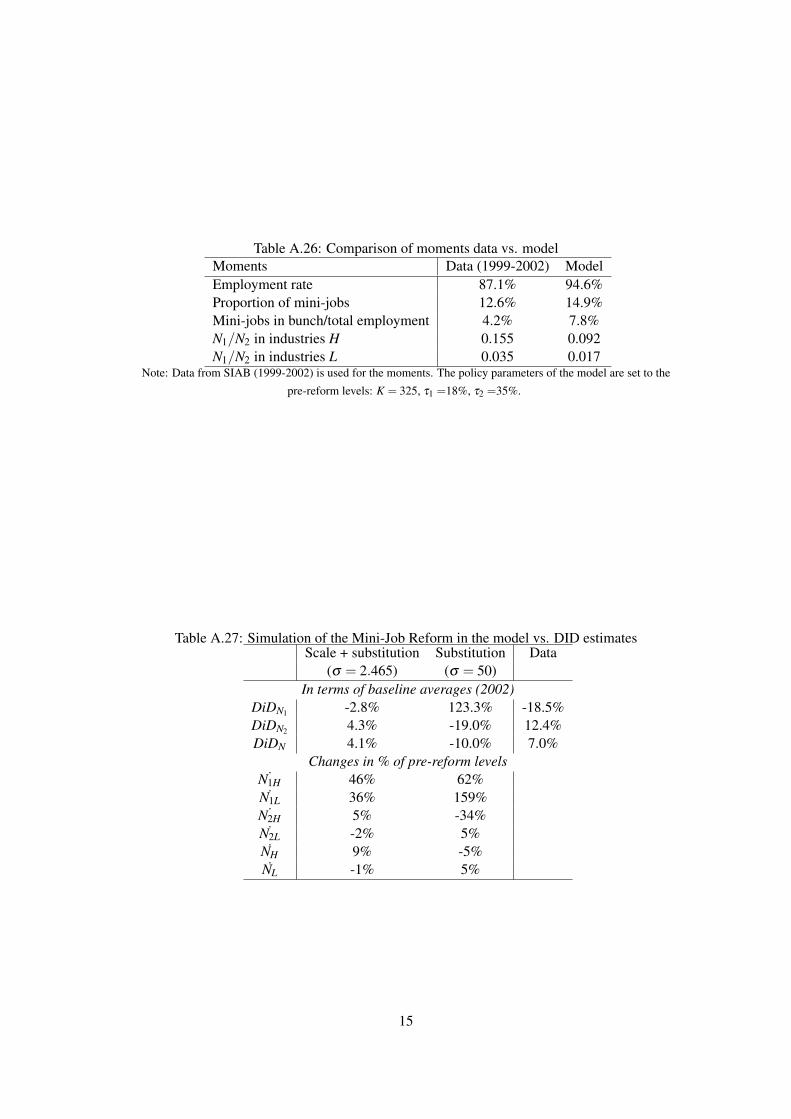
Table A.26: Comparison of moments data vs. modelMoments Data (1999-2002) ModelEmployment rate 87.1% 94.6%Proportion of mini-jobs 12.6% 14.9%Mini-jobs in bunch/total employment 4.2% 7.8%N1/N2 in industries H 0.155 0.092N1/N2 in industries L 0.035 0.017

Note: Data from SIAB (1999-2002) is used for the moments. The policy parameters of the model are set to the

pre-reform levels: K = 325, τ1 =18%, τ2 =35%.

Table A.27: Simulation of the Mini-Job Reform in the model vs. DID estimatesScale + substitution Substitution Data

(σ = 2.465) (σ = 50)In terms of baseline averages (2002)

DiDN1 -2.8% 123.3% -18.5%DiDN2 4.3% -19.0% 12.4%DiDN 4.1% -10.0% 7.0%

Changes in % of pre-reform levels˙N1H 46% 62%

N1L 36% 159%˙N2H 5% -34%

N2L -2% 5%NH 9% -5%NL -1% 5%

15

B Additional Figures

Figure B.1: Gross and net (of SSC) earnings of a worker as implied by the payroll tax schedulebefore (left) and after (right) the Mini-Job Reform

200 300 400 500 600 700 800 900 1000

Gross earnings

100

200

300

400

500

600

700

800

900

1000

Net

ear

ning

s

No taxRegular taxPre-reform tax schedule

200 300 400 500 600 700 800 900 1000

Gross earnings

100

200

300

400

500

600

700

800

900

1000

Net

ear

ning

s

No taxRegular taxPost-reform tax schedule

16

Figure B.2: Gross monthly earnings in 2000-2005P

ropo

rtio

n of

wor

kers

200 400 600 800 1000Gross monthly earnings

2000

Pro

port

ion

of w

orke

rs


2001

Pro

port

ion

of w

orke

rs


2002

Pro

port

ion

of w

orke

rs200 400 600 800 1000

Gross monthly earnings

2003

Pro

port

ion

of w

orke

rs


2004

Pro

port

ion

of w

orke

rs


2005

Source: SIAB, annual data, main spell, gross monthly earnings computed from daily wages.

Figure B.3: Employment rate and labor force participation

0.60

0.65

0.70

0.75

0.80

Sha

re o

f WA

P

1990 1995 2000 2005 2010 2015

Total employmentLabor force

Note: Data from DESTATIS. WAP stems for Working Age Population.

17

Figure B.4: Unemployment, non-employment and inactivity rate

0.25

0.30

0.35

0.40

Sha

re o

f WA

P

0.05

0.10

0.15

0.20

Sha

re o

f EA

P

1990 1995 2000 2005 2010 2015

Total unemployment (left axis)

Total non−employment (right axis)

0.22

0.24

0.26

0.28

0.30

Sha

re o

f WA

P

1990 1995 2000 2005 2010 2015

Inactivity rate

Note: Data from DESTATIS. EAP stems for Economic Age Population, and WAP for Working Age Population.

Figure B.5: Employment, full-time and part-time

0.40

0.45

0.50

0.55

0.60

0.65

0.70

0.75

0.80

Sha

re o

f WA

P

1990 1995 2000 2005 2010 2015

Total employment

Full−time employment

0.10

0.20

0.30

0.40

Sha

re o

f tot

al e

mpl

oym

ent

2000 2002 2004 2006 2008 2010

Part−time employment

Note: Data from DESTATIS. WAP stems for Working Age Population.

18

Figure B.6: Accounting exercise on the earnings distribution: expansion of in-work benefits

Figure B.7: Distribution of monthly gross earnings

Fre

quen

cy

200 400 600 800 1000 1200 1400 1600Gross monthly earnings

2000 2001

Fre

quen

cy

200 400 600 800 1000 1200 1400 1600Gross monthly earnings

2000 2002

Source: SIAB, annual, main spell, gross monthly earnings computed from daily wages.

19

Figure B.8: Cumulative distribution of monthly gross earnings

Cum

mul

ativ

e fr

eque

ncy


2002 2004

Only main job

Cum

mul

ativ

e fr

eque

ncy


2002 2004

All jobs

Source: SIAB, annual (left) and spell (right), gross monthly earnings computed from daily wages.

Figure B.9: Evolution of establishment-level employment

510

1520

2530

1999

2000

2001

2002

2003

2004

2005

2006

2007

Employment

510

1520

2530

1999

2000

2001

2002

2003

2004

2005

2006

2007

Full−time equivalent employment

Non−intensive in LE workers Intensive in LE workersTotal

Note: Panel 2000-2007. Intensive and non-intensive establishments in low-earning workers (LE) refer to whether they

are above or below the (weighted) median of the proportion of these workers.

20

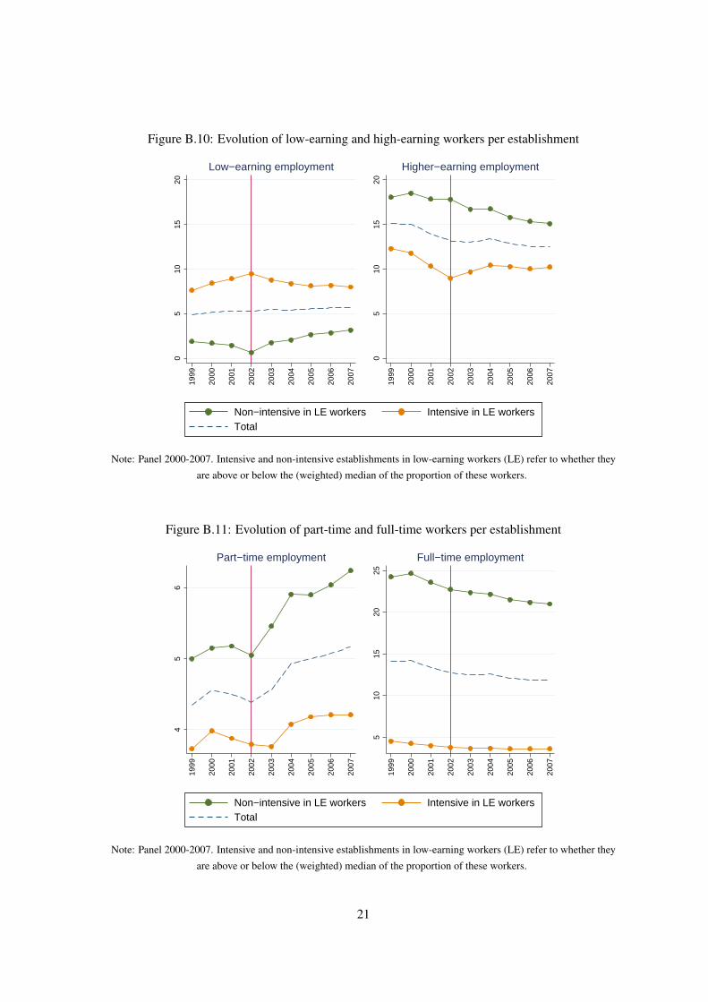
Figure B.10: Evolution of low-earning and high-earning workers per establishment

05

1015

20

1999

2000

2001

2002

2003

2004

2005

2006

2007

Low−earning employment

05

1015

20

1999

2000

2001

2002

2003

2004

2005

2006

2007

Higher−earning employment




Figure B.11: Evolution of part-time and full-time workers per establishment

45

6

1999

2000

2001

2002

2003

2004

2005

2006

2007

Part−time employment

510

1520

25

1999

2000

2001

2002

2003

2004

2005

2006

2007

Full−time employment




21

Figure B.12: Evolution of medium-educated and low-educated workers per establishment.0

8.0

9.1

.11

.12

.13

1999

2000

2001

2002

2003

2004

2005

2006

2007

Proportion of low−educated workers

510

1520

25

1999

2000

2001

2002

2003

2004

2005

2006

2007

Medium−educated employment




Figure B.13: Evolution of investment in physical capital per establishment

010

0000

2000

0030

0000

1999

2000

2001

2002

2003

2004

2005

2006

2007


Investment (euros)



22

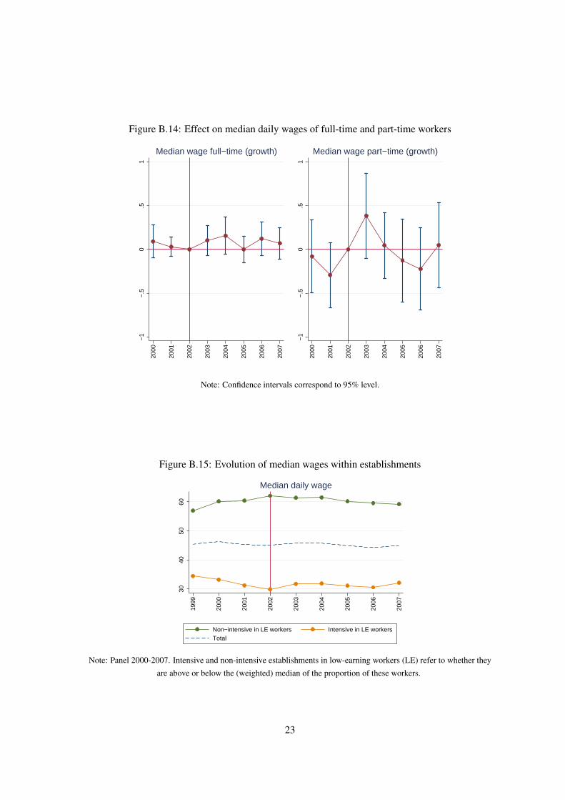
Figure B.14: Effect on median daily wages of full-time and part-time workers−

1−

.50

.51

2000

2001

2002

2003

2004

2005

2006

2007

Median wage full−time (growth)

−1

−.5

0.5

1

2000

2001

2002

2003

2004

2005

2006

2007

Median wage part−time (growth)

Note: Confidence intervals correspond to 95% level.

Figure B.15: Evolution of median wages within establishments

3040

5060

1999

2000

2001

2002

2003

2004

2005

2006

2007

Median daily wage




23

Figure B.16: Evolution of median wages within establishments, for full-time and part-time workers55

6065

7075

1999

2000

2001

2002

2003

2004

2005

2006

2007

Median daily wage full−time workers

1015

2025

3035

1999

2000

2001

2002

2003

2004

2005

2006

2007

Median daily wage part−time workers




Figure B.17: Effect on vacancies

−.5

0.5

1

2000

2001

2002

2003

2004

2005

2006

2007

Vacancies (log)


24

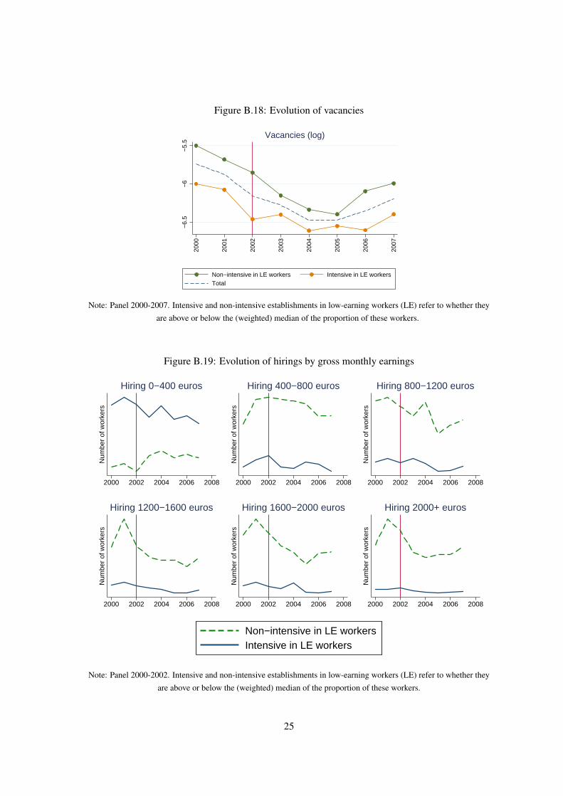
Figure B.18: Evolution of vacancies

−6.

5−

6−

5.5

2000

2001

2002

2003

2004

2005

2006

2007

Vacancies (log)




Figure B.19: Evolution of hirings by gross monthly earnings

Num

ber

of w

orke

rs

2000 2002 2004 2006 2008

Hiring 0−400 euros

Num

ber

of w

orke

rs

2000 2002 2004 2006 2008


Num

ber

of w

orke

rs

2000 2002 2004 2006 2008


Num

ber

of w

orke

rs

2000 2002 2004 2006 2008


Num

ber

of w

orke

rs

2000 2002 2004 2006 2008


Num

ber

of w

orke

rs

2000 2002 2004 2006 2008

Hiring 2000+ euros

Non−intensive in LE workersIntensive in LE workers



25

Figure B.20: Evolution of separations by gross monthly earnings

Num

ber

of w

orke

rs

2000 2002 2004 2006 2008

Separ. 0−400 euros

Num

ber

of w

orke

rs

2000 2002 2004 2006 2008


Num

ber

of w

orke

rs2000 2002 2004 2006 2008


Num

ber

of w

orke

rs

2000 2002 2004 2006 2008


Num

ber

of w

orke

rs

2000 2002 2004 2006 2008


Num

ber

of w

orke

rs

2000 2002 2004 2006 2008

Separ. 2000+ euros

Non−intensive in LE workersIntensive in LE workers



26

Figure B.21: Evolution of wage changes for workers within establishments

.4.4

5.5

.55

.6.6

5

2000

2001

2002

2003

2004

2005

2006

2007

Prop. workers with upgrade in earnings

.1.2

.3.4

2000

2001

2002

2003

2004

2005

2006

2007

Prop. workers with downgrade in earnings




Figure B.22: Effect on daily wages of workers flows with respect to average wage within the estab-lishment

−.5

0.5

11.

5R

atio

w.r

.t. a

vera

ge e

stab

lishm

ent w

age

2000

2001

2002

2003

2004

2005

2006

2007

Wage of hirings/average wage

−.5

0.5

11.

5R

atio

w.r

.t. a

vera

ge e

stab

lishm

ent w

age

2000

2001

2002

2003

2004

2005

2006

2007

Wage of separations/average wage


27

Figure B.23: Evolution of occupational structure (proportion of workers in each task, and numberof job titles)

.08

.1.1

2.1

4.1

6

1999

2000

2001

2002

2003

2004

2005

2006

2007

Analytical non−routine

.09

.1.1

1.1

2.1

3.1

4

1999

2000

2001

2002

2003

2004

2005

2006

2007

Interactive non−routine

.32

.34

.36

.38

.4

1999

2000

2001

2002

2003

2004

2005

2006

2007

Cognitive routine.0

6.0

8.1

.12

1999

2000

2001

2002

2003

2004

2005

2006

2007

Manual routine.2

8.2

9.3

.31

.32

1999

2000

2001

2002

2003

2004

2005

2006

2007

Manual non−routine

33.

54

4.5

5

1999

2000

2001

2002

2003

2004

2005

2006

2007

Number of job titles


Figure B.24: Effects on employment, model with LDV

−1

01

2000

2001

2002

2003

2004

2005

2006

2007

Conf. int. Blundell−Bond

OLS Within

Total employment

−1

−.5

0.5

1

2000

2001

2002

2003

2004

2005

2006

2007


OLS Within

Total full−time equivalent employment

Note: Confidence intervals correspond to 95% level, only reported for Blundell-Bond estimates. Hansen statistic for

overidentifying restrictions is not significant for full-time employment (at the 5% level), but it is for employment.

Differences-in-Hansen statistics for tests of validity of both GMM and IV instruments are not significant for full-time

employment, and only for IV instruments for employment. Hypothesis of autocorrelation of residuals for more than 1

period is rejected (at the 5% level for employment and at any level for full-time equivalent employment).

28

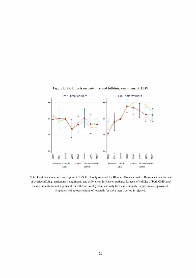
Figure B.25: Effects on part-time and full-time employment, LDV

−2

−1

01

2000

2001

2002

2003

2004

2005

2006

2007


OLS Within

Part−time workers

−2

−1

01

2000

2001

2002

2003

2004

2005

2006

2007


OLS Within

Full−time workers

Note: Confidence intervals correspond to 95% level, only reported for Blundell-Bond estimates. Hansen statistic for test

of overidentifying restrictions is significant, and differences-in-Hansen statistics for tests of validity of both GMM and

IV instruments are not significant for full-time employment, and only for IV instruments for part-time employment.

Hypothesis of autocorrelation of residuals for more than 1 period is rejected.

29

Figure B.26: Effects on employment by education level, LDV

−.0

6−

.04

−.0

20

.02

.04

2000

2001

2002

2003

2004

2005

2006

2007


OLS Within

Proportion of low−educated workers

−1

−.5

0.5

1

2000

2001

2002

2003

2004

2005

2006

2007


OLS Within

Medium−educated workers

Note: Confidence intervals correspond to 95% level, only reported for Blundell-Bond estimates. Hansen statistic for test

of overidentifying restrictions is not significant for medium-educated workers, and it is significant for low-educated

workers. Differences-in-Hansen statistics for tests of validity of both GMM and IV instruments are not significant for

both. Hypothesis of autocorrelation of residuals for more than 1 period is rejected.

Figure B.27: Distribution of establishments according to the proportion of low-earning workers,2002 vs. 2007

Pro

port

ion

of e

stab

lishm

ents

(%

)

0 .2 .4 .6 .8 1Low−earning workers / total employment

2002 2007

Note: LIAB, panel 2000-2007.

30

Figure B.28: Earnings distribution by establishment pre-reform intensity in low-earning workers,2002 vs. 2004

Fre

quen

cy

0 200 400 600 800 1000Euros/month

Quintiles 1 and 2, 2002

Fre

quen

cy

0 200 400 600 800 1000Euros/month


Fre

quen

cy

0 200 400 600 800 1000Euros/month

Quintile 3, 2002

Fre

quen

cy

0 200 400 600 800 1000Euros/month

Quintile 3, 2004

Fre

quen

cy

0 200 400 600 800 1000Euros/month


Fre

quen

cy

0 200 400 600 800 1000Euros/month


Note: LIAB, panel 2000-2007. Quintiles are defined according to the intensity in 2002, and establishments are followed

to 2004

Figure B.29: Proportion of establishments by intensity in low-earning workers, panel 2000-2007

58.2

41.8

60.6

39.4

65.5

34.5

62.3

37.7

53.8

46.2

53.7

46.3

48.9

51.1

52.0

48.0

2000 2001 2002 2003 2004 2005 2006 2007

Services for businesses

57.5

42.5

60.3

39.7

59.7

40.3

58.1

41.9

56.5

43.5

57.7

42.3

57.1

42.9

52.6

47.4

2000 2001 2002 2003 2004 2005 2006 2007

Other services

57.1

42.9

58.8

41.2

61.8

38.2

55.3

44.7

55.1

44.9

55.7

44.3

52.8

47.2

51.5

48.5

2000 2001 2002 2003 2004 2005 2006 2007

Retail, repair

45.9

54.1

43.0

57.0

43.4

56.6

42.0

58.0

45.3

54.7

43.8

56.2

40.3

59.7

40.2

59.8

2000 2001 2002 2003 2004 2005 2006 2007

Manufacturing

30.9

69.1

31.2

68.8

33.5

66.5

33.2

66.8

27.1

72.9

33.4

66.6

32.4

67.6

32.4

67.6

2000 2001 2002 2003 2004 2005 2006 2007

Construction

37.7

62.3

41.6

58.4

42.2

57.8

36.6

63.4

40.2

59.8

40.6

59.4

37.4

62.6

40.6

59.4

2000 2001 2002 2003 2004 2005 2006 2007

Transport, communication

27.1

72.9

34.1

65.9

32.7

67.3

30.6

69.4

28.3

71.7

38.3

61.7

38.4

61.6

50.0

50.0

2000 2001 2002 2003 2004 2005 2006 2007

Agriculture, primary

42.4

57.6

49.0

51.0

46.4

53.6

45.1

54.9

45.0

55.0

43.0

57.0

43.9

56.1

43.6

56.4

2000 2001 2002 2003 2004 2005 2006 2007

Public sector

Intensive Non−intensive

Note: LIAB, panel 2000-2007. Intensive establishments are those with a proportion of low-earning workers above the

annual median, and non-intensive as those with proportion of low-earning workers below the annual median. Financial

intermediation excluded due to insufficient number of observations.

31

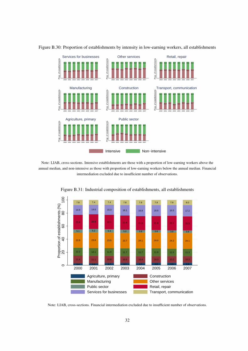
Figure B.30: Proportion of establishments by intensity in low-earning workers, all establishments

48.6

51.4

47.6

52.4

50.9

49.1

51.0

49.0

52.0

48.0

53.7

46.3

50.5

49.5

53.2

46.8

Pro

p. o

f est

ablis

hmen

ts

2000 2001 2002 2003 2004 2005 2006 2007

Services for businesses

62.1

37.9

61.3

38.7

57.2

42.8

64.3

35.7

62.7

37.3

64.3

35.7

60.9

39.1

64.4

35.6

Pro

p. o

f est

ablis

hmen

ts

2000 2001 2002 2003 2004 2005 2006 2007

Other services

54.5

45.5

56.0

44.0

55.4

44.6

56.3

43.7

54.5

45.5

57.9

42.1

54.4

45.6

55.8

44.2

Pro

p. o

f est

ablis

hmen

ts

2000 2001 2002 2003 2004 2005 2006 2007

Retail, repair

46.7

53.3

46.7

53.3

46.4

53.6

44.8

55.2

46.2

53.8

46.6

53.4

42.4

57.6

46.8

53.2

Pro

p. o

f est

ablis

hmen

ts

2000 2001 2002 2003 2004 2005 2006 2007

Manufacturing

32.6

67.4

33.2

66.8

34.4

65.6

36.8

63.2

34.5

65.5

39.6

60.4

34.2

65.8

41.7

58.3

Pro

p. o

f est

ablis

hmen

ts

2000 2001 2002 2003 2004 2005 2006 2007

Construction

45.7

54.3

41.5

58.5

45.3

54.7

36.0

64.0

40.8

59.2

46.3

53.7

42.9

57.1

45.7

54.3

Pro

p. o

f est

ablis

hmen

ts

2000 2001 2002 2003 2004 2005 2006 2007

Transport, communication

39.4

60.6

35.9

64.1

39.0

61.0

42.8

57.2

38.3

61.7

40.8

59.2

41.0

59.0

44.3

55.7

Pro

p. o

f est

ablis

hmen

ts

2000 2001 2002 2003 2004 2005 2006 2007

Agriculture, primary

40.8

59.2

47.3

52.7

50.2

49.8

46.1

53.9

41.6

58.4

42.6

57.4

42.3

57.7

41.3

58.7

Pro

p. o

f est

ablis

hmen

ts

2000 2001 2002 2003 2004 2005 2006 2007

Public sector

Intensive Non−intensive

Note: LIAB, cross-sections. Intensive establishments are those with a proportion of low-earning workers above the

annual median, and non-intensive as those with proportion of low-earning workers below the annual median. Financial

intermediation excluded due to insufficient number of observations.

Figure B.31: Industrial composition of establishments, all establishments

3.4

11.4

12.2

22.8

5.1

22.4

14.9

7.8

3.3

11.1

12.1

23.8

5.2

22.5

14.6

7.4

3.7

10.8

11.9

23.5

5.3

22.1

15.3

7.4

3.7

10.5

11.7

23.7

5.0

21.6

16.1

7.8

3.7

10.4

11.7

24.1

3.8

21.5

16.8

7.9

3.8

10.3

11.9

24.0

3.8

21.6

16.6

7.9

3.9

10.2

11.5

24.2

3.8

22.1

16.5

7.8

3.9

10.3

11.3

24.1

3.8

21.5

17.2

8.0

020

4060

8010

0P

ropo

rtio

n of

est

ablis

hmen

ts (

%)

2000 2001 2002 2003 2004 2005 2006 2007

Agriculture, primary ConstructionManufacturing Other servicesPublic sector Retail, repairServices for businesses Transport, communication

Note: LIAB, cross-sections. Financial intermediation excluded due to insufficient number of observations.

32

Figure B.32: Proportion of low-earning workers by commuting zones in 2002

(.1771934,.2342626](.1623718,.1771934](.1345116,.1623718][.0938389,.1345116]

2002

Note: SIAB data. Values for commuting zones of residence.

Figure B.33: Variation (in pp.) in the proportion of low-earning workers by commuting zones

(.0179318,.0429869](.0141342,.0179318](.0090349,.0141342][−.0131299,.0090349]

Var. 2002−2004 in p.p.

Note: SIAB data. Values for commuting zones of residence.

Note: Confidence intervals correspond to 95% level, only reported for Blundell-Bond estimates.

33

C Additional Details on the Data

I perform a set of preparation and cleaning procedures in both the SIAB and the LIAB whichfollows the recommendations and instructions provided by the IAB. First, I correct for the excessmissing values and inconsistencies in the education variables, due to the fact that the reporting ofthese variables is done by employers but it has not consequences for social security. I follow thecriterium “2B” in Fitzenberger, Osikominu, and Volter (2005), which uses all the information forthe same individual (forward and backward extrapolation, assignment of the maximum value forparallel spells), and considers the possibility of both under and over reporting. I adapt the codeprovided by the IAB, by using information coming from unemployment or training spells as well.

Another important adjustment I perform is imputation of daily earnings when they are right cen-sored (above the social security contribution limit). Right censoring affects fewer than 5% of theobservations and, in particular, it does not affect low-earning workers. The definition of low-earningand high-earning workers, crucial for the firm level analysis, is binary and hence does not incorpo-rate measurement error coming from this limitation. However, to count with a reliable measure ofearnings, I impute top coded wages using a series of Tobit models to log-daily earnings by educationand age groups following the methodology in Card, Heining, and Kline (2013) (see also Dustmann,Ludsteck, and Schonberg 2009 and Gartner 2005) adapted to processing constraints imposed byremote and on-site access of the data. The uncensored imputed value is the prediction of the modelaccording to the covariates. I use four groups of education (no degree or primary/lower secondaryor intermediate school leaving certificate without vocational training, intermediate school leavingcertificate with vocational training -“apprentices”-, upper secondary school certificate - “Abitur” -with or without vocational certificate, and degree from technical school or University) and sevenage groups of 10 year-range (in the first I include all people below 20 and in the last, all above 80years old). The explanatory variables include age in years, an indicator for firms with more than 10employees, the average proportion of right censored observations and average log daily wage withinthe establishment, a second degree polynomial of the number of workers at the establishment, anindicator for unipersonal establishments, the average proportion of workers with university degreeand the average years of schooling by establishment.

An important feature of the SIAB is that it is spell data, which means that every time there is anotification by the employer (annually, or in the event of changes in contribution group or healthinsurance company, or changes in the payroll system of the employer), or a change in the status asrecipient of unemployment benefits or as job seeker, a new observation is added to the data-set. Iuse spell data in particular to compute transitions between states witin employment, and to and fromunemployment. In such cases, I consider all the spells during each year of the time series. Someof the descriptives are based on a transformation of the data to annual frequencies, according to themethodology proposed by the IAB. I keep all the spells which contain June 30 each year. I furtherrestrict to one spell per worker-year (I eliminate parallel spells) for some of the descriptives, keepingthe observation with highest amount of earnings or benefit reception. I explicit which version of thedata I use in each case: “spell data”, “annual data”, or “annual data, main spell” respectively. Finally,I do not consider employment spells with 0 daily earnings.

With respect to the LIAB, I do not impose exclusions of any type on establishments. Typical ex-clusions in the literature vary according to the topic, and consist of excluding small establishments(17% of the establishments in the Establishment Panel have two employees), establishments in theagricultural sector (6.7%) and in the public administration (9.6%). I avoid restrictions as the sampleis meant to be representative of all establishments in Germany. Furthermore, I am agnostic about

34

how establishments typically excluded in the literature affect the results.

Regarding the variables used in the analysis, the data from IEB contains direct report of whetherthe employment spell comes from regular employment, mini-job (“marginal part-time”) or midi-job(“in transition zone”), and I use this definition for the descriptives. I use monthly gross earnings, inparticular for the definition of intensity in low-earning workers at the establishment level (propor-tion of workers in the pre-reform year who were below the after-reform threshold in earnings) andfor the analysis of the earnings’ distributions. As the data only provides daily (in calendar days)earnings, I generate a monthly conversion following Tazhitdinova (2017). For workers with a singleemployment spell covering the whole year, I multiply the daily earnings by the average number ofdays in a month (30.4). For individuals with multiple employment periods in a year, I computeaverage daily earnings in the year, and I multiply it by the average number of days in a month.

Full-time equivalent employment, as a proxy for hours, is constructed by attributing a weight below1 to part-time workers. In particular, IEB differentiates between “mini” part-time workers (hoursworked below half full-time, corresponding to 18 hours a week), and “midi” part-time workers(hours worked above half full-time and below full-time). I assign a weight of 0.5 to “mini” part-time workers, and 0.75 to “midi” part-time workers. Even though weights are somewhat arbitrary, Iconfirm that results are the same if I change the weights (for eg., assigning 0.25 to “mini” part-timeemployment and 0.5 to “midi” part-time workers).

Regarding the classifications used along the analysis, I use the most recent time-consistent industryclassification provided by the IAB (Classification of Economic Activities, 1993 version, 3-digits,224 categories). I perform groupings of this classification for some of the analysis, where I indicateit. Occupations are categorized according to the German Classification of Occupations (KldB) 1988,comprising 344 categories, and are grouped according to complexity and routinization followingDengler, Matthes, and Paulus (2014). The classification is based on the BERUFENET data collectedby IAB containing expert knowledge about competencies and skills. For the definition of local labormarkets, I use the classification of districts (“kreis”) in commuting zones in Kosfeld and Werner(2012).

Finally, the response rate in the IAB Establishment Panel is stable over the years and higher than80%. For longitudinal analysis, the IAB constructs several longitudinal sections, with the corre-sponding weights. These sections, besides including new establishments and establishments go-ing out of operation, keep the establishments which have continuity in the response to the surveyfrom one year to the next, being then free of survey non-response. I focus on the longitudinalsection 2000-2007 which is the most suitable for the period of the reform. I provide some descrip-tives though using the cross-section of the Establishment Panel, duely clarified in the text. Eventhough there is no survey non-response in the longitudinal analysis, the survey is subject to itemnon-response by certain establishments. However, most of the variables in the analysis such as em-ployment, wages, occupations and industries are drawn from the social security records from IEBand BHP linked to the Establishment Panel.1 I consider therefore that measurement error is not amajor issue for the analysis in this paper.

1One important exception is investment, which is reported by establishments in the survey and it is subject to non-negligible item non-response.

35

D Additional Derivations

D.1 Accounting exercise on the earnings distributionFigure (B.6) explains schematically the main ideas for this exercise. Let’s denote the change in themass of workers below the mini-job threshold as follows:

∆Emp(MJ)≡ Emp1(MJ)−Emp0(MJ)Emp0(MJ)

(1)

where Empt(MJ) denotes employment below earnings threshold introduced by the reform (e400),and t is 0 for before and 1 for after. The mass is normalized by the employment level belowthe threshold in case of absence of reform. The mass below the threshold after the reform com-prises: (1) workers who retain their job (potentially improving earnings), (2) workers who transitfrom non-employment to employment, denoted by Emp+1 (MJ), and (3) workers pulled from abovethe earnings distribution, Emp−1 (MJ). Decomposing Emp1(MJ) into the sum of Emp+1 (MJ) andEmp−1 (MJ)

∆Emp(MJ) =Emp+1 (MJ)+Emp−1 (MJ)−Emp0(MJ)

Emp0(MJ)(2)

The fraction of entrants from non-employment is then:

∆Emp+MJ ≡Emp+1 (MJ)−Emp0(MJ)

Emp0(MJ)= ∆Emp(MJ)−

Emp−1 (MJ)Emp0(MJ)

(3)

which is the excess mass of workers below the threshold netted out from the proportion pulled down.The fraction of workers coming from the upper segment of the earnings distribution is proxied bythe missing mass close to the threshold:

Emp−(MJ)≡ emp0(w > MJ)− emp1(w > MJ) (4)where empt(w > MJ) denotes the number of workers with wages above the mini-job threshold.Using annual data (considering individuals only according to the main job), and e1,200 as upperlimit (where visually the pre and post reform distributions of earnings converge), the quantities are:∆Emp(MJ)/Emp0(MJ)=7.8% and Emp−(MJ)/Emp0(MJ)=-4.1%, which yields ∆Emp+MJ =3.6%.This excess mass is even larger when considering only the prime-age population (9.8%), and moreso if all spells (secondary jobs included) are considered (41.7%).

D.2 Derivations regarding the theoretical framework

D.2.1 Partial equilibrium: Labor supply decision

The first order condition for the solution of the problem (10) in the absence of non-linearities is:n = αwε (5)

Note that w = α−1ε n

1ε , is positively related to the disutility of work. Net earnings, α−

1ε n

1+ε

ε , are anot-linear function of hours.2 The take-home wage of the worker is below her productivity, w < w,as a consequence of the tax.

With non-linear taxes, wages, fixed costs of work and non-labor income, there exists α∗0 such thatU(b,0) =U(c,n) (for n > 0):

α∗0 =

(ε +1)(b+β )

wε+11

(6)

Let’s define α∗1 as the value of α such that workers choose n which yields K before-tax earnings (K2The formulation with non-linear earnings in function of hours is typical in the literature dealing with intensive and

extensive margins of labor supply (see for eg. Erosa, Fuster, and Kambourov 2016). Note that earnings are increasing inthe disutility for labor, to compensate the individual for the utility cost of supplying more hours of work. The non-linearspecification penalizes individuals with low number of hours, bounding intensive margin decisions away from zero.

36

after taxes):

α∗1 ≡

Kwε+1

1(7)

Finally, there exists α∗2 that solves U(K, K/w1) =U(αwε+12 ,αwε

2):

(ε +1)K− εα∗− 1

ε

2

(Kw1

)1+ 1ε

−α∗2 wε+1

2 = 0 (8)

Let us consider the relevant case of w1 > w2. For individuals with α ≤ α∗0 , the fixed cost of workingand the loss of non-labor income are sufficiently high that the net earnings in job type 1 cannotcompensate for them, if they were to supply their preferred number of hours, and as a consequencethey do not work. For α∗0 < α ≤ α∗1 , individuals optimally choose their number of hours and sortinto jobs type 1, with α∗1 corresponding to the individual for which the optimal n is such that grossearnings are exactly K. Individuals with α∗1 < α < α∗2 would like to work more hours at the take-home wage w1, but cannot do it because their earnings would surpass K and the wage they receiveis w2 < w1. These agents bunch at the threshold supplying n = K/w1 at w1 and subject to τ1.Individuals with α ≥ α∗2 supply their optimal number of hours at w2 and are subject to τ2.

D.2.2 Comparative statics: change in labor supply when tax benefits change

Given w1 and w2, when τ1 decreases, (1− τ1) increases one to one. The change in α∗0 is:∂α∗0

∂ (1− τ1)=− (ε +1)2(b+β )

(1− τ1)ε+2wε+11

(9)

which is negative. For α∗1 :∂α∗1

∂ (1− τ1)=− εK

wε+11

(10)

is also negative. For α∗2 , renaming equation (8) as the implicit function F(α∗2 ,(1− τ1)):∂α∗2

∂ (1− τ1)=−∂ F/∂ (1− τ1)

∂ F/∂α∗2(11)

where:∂ F

∂ (1− τ1)= (ε +1)K (12)

∂ F∂α∗2

= α∗− 1

ε−1

2

(Kw1

)1+ 1ε

− wε+12 (13)

Equation (12) is positive. To derive the sign of equation (13), note that the first term is lower thanthe second because: (

Kα∗2 wε+1

1

) 1ε

<w2

w1(14)

α∗2 wε+11 are the net earnings the individual with the initial α∗2 would have if she could supply the

optimal number of hours at w1, which are higher than K by construction. The factor in the left handside is hence lower than one, the same as the factor in the right hand side as we are in the case wherew2 < w1. Besides, the exponent 1/ε > 1 means that the left hand side is smaller than the right handside. Hence, expression (13) is negative and ∂α∗2/∂ (1−τ1)> 0. As a consequence of the expansionof the in-work benefit (modelled as a decrease in τ1), given the wages, NS

1 increases due to both theinflow of new entrants into employment (α∗0 decreases) and workers previously in jobs type 2 (α∗2increases), whereas NS

2 decreases, pushing upwards the ratio NS1/NS

2 in partial equilibrium.

This parsimonious way of modelling the expansion of an in-work benefit, by a reduction in τ1,is illustrative but does not follow exactly the Mini-Job Reform case. With the reform, K increased

37

leaving τ1 virtually unaffected. The result of this modification is also an increase in NS1/NS

2 in partialequilibrium, but the channel is different. α∗0 does not change, whereas:

∂α∗1∂K

=1

wε+11 (1− τ1)ε

(15)

is positive, and:∂α∗2∂K

=− ∂ F/∂K∂ F/∂α∗2

(16)

is also positive. Note that in equation (16) the denominator is the same as in equation (11), and thenumerator is:

∂ F∂K

= (ε +1)(1− τ1)− εα∗− 1

ε

2

(1+

1ε

)(Kw1

) 1ε

(17)

For this expression to be positive, (1−τ1)εwε+1

1 α∗2 >K. This is indeed the case because the left handside is the total before-tax earnings of individual with α∗2 if she were to supply her preferred hoursat the take-home wage w1. This amount is higher than K by construction. Hence, equation (16)is positive. This means that the change in NS

1/NS2 with the Mini-Job Reform under this framework

responds exclusively to a reallocation of workers, both within the low-earning sector (the increase inα∗1 means that workers already in jobs type 1 supply more hours), and coming from the high-earningsector (the increase in α∗2 captures that workers previously in jobs type 2 sort into jobs type 1 byreducing hours). Although this effects are not unreasonable for many workers, there is a dimensionthe model is missing: the entry from secondary workers who may have higher fixed costs of workand would be induced to enter after the reform given the higher net wage. There is also new low-earning jobs taken up as second job, something also not captured in the model. These caveats areimportant, as pointed out in section (3.2). Although I do not introduce them in the model yet, Iconsider them when discussing the results from the quantitative exercise.

D.2.3 Equilibrium wages

As previously showed, the expansion of an in-work benefit induces NS1/NS

2 to increase. In equi-librium, supply and demand for each of the jobs, and relative wages, need to adjust for the labormarket to clear. These changes are simultaneous but I show them sequentially. I first use the factthat ND

1 /ND2 needs also to increase to match the labor supply, to show the direction of the change in

the firm-specific intensities. And then I show that w1/w2 will fall to accommodate the changes inquantities.

From the first order condition in equation (2), it must hold:(θH

1−θH

)−σ N1H

N2H=

(θL

1−θL

)−σ N1L

N2L(18)

Taking derivatives in both sides with respect to ND1 /ND

2 :(θH

1−θH

)σ∂ (N1H/N2H)

∂ (ND1 /ND

2 )=

(θL

1−θL

)σ∂N1L/N2L

∂ND1 /ND

2(19)

Equation (19) shows that the direction of change in the intensities of each firm is the same as in theaggregate intensity because θk/(1−θk)> 0. For a higher ND

1 /ND2 to match the increase NS

1/NS2 due

to the expansion of the tax benefit, the firm-specific intensities need to increase.

Knowing that the firm-specific intensity moves in the same direction as the aggregate intensityin labor demand, without loss of generality I can derive the direction of the change in w1/w2 inequilibrium, by deriving both sides of the first order condition for the firm H with respect to the

38

change in NS1/NS

2 , which in equilibrium is equal to the change in ND1 /ND

2 :

∂ (w1/w2)

∂ (ND1 /ND

2 )=− 1

σ

(θH

1−θH

)(N1H

N2H

)− σ+1σ ∂ (N1H/N2H)

∂ (ND1 /ND

2 )(20)

All the factors in the right hand side have a positive sign, except for −1/σ < 0. Hence, for ND1 /ND

2to increase to equate the labor supply, w1/w2 needs to fall. Note that the lower is σ (the morecomplements are low-earning and high-earning workers), the bigger the response on wages due to achange in the relative supply, and the smaller the changes in relative quantities. On the other hand,the only case in which the change in the relative supply does not exert any effect on relative wagesis when low-earning and high-earning jobs are perfect substitutes (σ → ∞).

D.2.4 Decomposition in scale and substitution effect

The Hicks-Marshall rules of derived demand allow to decompose the change in the labor demandof each task when there is a change in the price of one input, in terms of elasticities and cost factorshares. Let’s assume perfect competition and free entry.3 For simplicity, I skip the index for thefirm k, but all derivations need to hold for both k ∈ {H,L}.

Let s1 ≡ w1N1pY = θ

(N1Y

) σ−1σ and s2 ≡ w2N2

pY = (1−θ)(N2

Y

) σ−1σ be the cost share of labor in type-1 and

type-2 jobs respectively.

Totally differentiating Y = F(N1,N2):

dY = Y1σ θN

− 1σ

1 dN1 +Y1σ (1−θ)N

− 1σ

2 dN2

dYY =

Y1σ θN

− 1σ

1 N1Y

dN1N1

+Y

1σ (1−θ)N

− 1σ

2 N2Y

dN2N2

dlnY = s1dlnN1 + s2dlnN2

(21)

Since the production function is constant returns to scale, s1 = 1− s2:dlnY = s1dlnN1 +(1− s1)dlnN2

dlnN1 = dlnY +(1− s1)(dlnN1−dlnN2)(22)

Dividing by dlnw1:dlnN1

dlnw1=

dlnYdlnw1

+(1− s1)dlnN1−dlnN2

dlnw1(23)

A similar expression can be derived for N2:dlnN2

dlnw1=

dlnYdlnw1

− s1dlnN1−dlnN2

dlnw1(24)

These expressions decompose the change in the demand for both factors N1 and N2 when the priceof one of them changes, w1, in a scale effect (first term) and a substitution effect (second term).Whereas the scale effect has the same direction in both the demand of N1 and N2, the substitutioneffect acts in opposite direction.

Next, I express equations (23) and (24) in terms of elasticities. For the scale effect, I use the fact thatunder perfect competition and free entry, firms make zero-profits: pY = w1N1 +w2N2. Defining asη ≡−dlnY

dlnp the elasticity of demand for output (in absolute value), and plugging dlnY =−ηdlnp inequation (23):

dlnN1

dlnw1=−η

dlnpdlnw1

+ s2dlnN1−dlnN2

dlnw1(25)

Differentiating the zero-profit condition, for the case that only w1 changes, and using equation (21):dlnp = s1dlnw1 (26)

3Harasztosi and Lindner (2017) derive an analogous decomposition under imperfect competition.

39

For the substitution effect, using the ratio of first order conditions of the firm’s problem:N1

N2=

(θ

1−θ

)σ (w1

w2

)−σ

(27)

Taking logs and differentiating:dlnN1−dlnN2 =−σdlnw1 (28)

The elasticities of the demand for labor in each type of jobs when the price of type-1 jobs changesare:

dlnN1dlnw1

=−[s1η +(1− s1)σ ]dlnN2dlnw1

=−[s1η− s1σ ](29)

D.2.5 Intensities and cost-shares

From the first order conditions of the firm, N1HN2H

> N1LN2L

. From the definition of s1 omitting the indicesk.

s1 = θ(N1

Y

) σ−1σ

= θ

{A

[θ +(1−θ)

(N1N2

)− (σ−1)σ

]}−1 (30)

Deriving with respect to N1/N2:

∂ s1

∂ (N1/N2)= θ(1−θ)

σ −1σ

(N1

N2

)− 2σ−1σ

θ +(1−θ)

(N1

N2

)− (σ−1)σ

−2

(31)

where the right hand side is positive.

Let’s define φk ≡ N1kN1k+N2k

as the proportion of hours in the firm by low-earning workers out of totalnumber of hours. I skip the k indices, and express N1/N2 in terms of φ :

N1

N2=

φ

1−φ(32)

Deriving this expression in terms of φ

∂ (N1/N2)

∂φ=

11−φ

(33)

which is a positive expression, as ∂ s1/∂ (N1/N2) showed before. Hence:∂ s1

∂φ=

∂ s1

∂ (N1/N2)

∂N1/N2

∂φ> 0 (34)

The insight from this expression is that there is a positive relationship between the cost-share, whichis the relevant variable when considering the heterogenous strength of scale and substitution effects,and the fraction of labor in low-earning jobs, closely related to the variable used in the empiricalanalysis.

D.2.6 Consumption and government budget

Aggregate income is:Inc = (b+ tr)F(α∗0 )

+∫ α∗1

α∗0(αwε+1

1 + tr) f (α)dα +∫ α∗2

α∗1(K + tr) f (α)dα

+∫

∞

α∗2(αwε+1

2 + tr) f (α)dα

(35)

Total income in the economy is exhausted in the demand for goods: Inc = pHYH +YL. I model thedemand for each good using a CES aggregator at the economy-wide level.

YH = 1pH

Inc1+pκ−1

HYL = Inc

1+pκ−1H

(36)

40

Balance of the government budget implies T = G, where:T =

∫ α∗1α∗0

αwε+11 (1− τ1)

ετ1 f (α)dα +∫ α∗2

α∗1Kτ1 f (α)dα

+∫

∞

α∗2αwε+1

2 (1− τ2)ετ2 f (α)dα

(37)

and:G = tr+bF(α∗0 ) (38)

D.2.7 Parameterization and solution

To solve the model, I start in partial equilibrium (w1 and w2 fixed), and I obtain NS1 and NS

2 , Inc,YH , YL, N1H , N1L, N2H , and N2L. Using the zero-profit condition of the firm H, I further obtain pH .Finally, I iterate on w1 and w2 until the excess supply for both types of job is zero.

The parameters for the labor demand are selected as follows. I estimate an industry-level regressionusing the first order conditions of the firms (in logs):

ln(

N1it

N2it

)= λi−σ ln

(w1it

w2it

)+πt +ξit (39)

where i is the industry (224 categories). I use data from LIAB, cross-section, for the period 1999-2000. I measure N1it and N2it as the annual average by industry of the total full-time equivalentemployment in the low-earning and high-earning segment respectively (as before, I use the post-reform mini-job threshold for this definition). I measure w1it and w2it in a similar way, correspondingto the industry-level average of the full-time equivalent daily wage of workers in each group. Ifurther include a linear trend. Expression (39) allows to retrieve an estimation of the parameter σ .In order to address the endogeneity due to the omission of important variables in the productionfunction (such as capital for example, not directly available in the data), I instrument ln

(w1ktw2kt

)with a Post indicator, that takes the value 1 for the years after the reform. The estimation suggestsσ = 2.462, higher than for a Cobb-Douglas specification and low enough such that low-earning andhigh-earning workers are not perfect substitutes.

I retrieve the parameters θk using the fixed effects in the regression, and their correspondence withthe model specification: λi = σ ln

(θi

1−θi

). I take the average for the industries which were above

the median in the proportion of low-earning workers in 2002 to obtain θH , and the similarly butfor below median industries to obtain θL. I further estimate the CES specification of the productionfunction using the parameters retrieved, the sales in real terms as measures for Yit , and the employ-ment measures (all normalized for the year 2002), from which I obtain the relation of magnitudesbetween AH and AL using averages across industries similar as before. This exercise suggests thatAL is 5% higher than AH . The values obtained in this way imply that θH > θL and AH < AL, whichis sensible since H firms are intensive in low-earning workers and they are likely to have lower totalfactor productivity.

For the labor supply side of the model, I assume F(α) follows a Weibull distribution, characterizedby parameters µ and γ . The parameter ε is set to the average of estimates by Tazhitdinova (2017).The rest of the parameters (β , µ , γ , b, κ) are selected such that the model provides reasonableapproximations to the employment rate, the proportion of mini-jobbers with respect to the totalnumber of workers, the proportion of workers in the bunching at e400, and the average acrosshighly intensive and low intensity (as of 2002) establishments. Parameters values are shown intable (A.25) and the comparison of the moments of the model, in table (A.26).

41

References

Card, D., J. Heining, and P. Kline (2013). Workplace heterogeneity and the rise of West Germanwage inequality. Quarterly Journal of Economics 128(3), 967–1015.

Dengler, K., B. Matthes, and W. Paulus (2014). Occupational tasks in the German labour market.An alternative measurement on the basis of an expert database. Methodenreport 12/2014, Re-search Data Center (FDZ) of the German Federal Employment Agency (BA) at the Institutefor Employment Research (IAB).

Dustmann, C., J. Ludsteck, and U. Schonberg (2009). Revisiting the German wage structure.Quarterly Journal of Economics 124(2), 843–881.

Erosa, A., L. Fuster, and G. Kambourov (2016). Towards a micro-founded theory of aggregatelabor supply. Review of Economic Studies 83.

Fitzenberger, B., A. Osikominu, and R. Volter (2005). Imputation rules to improve the educa-tion variable in the IAB employment subsample. FDZ Methodenreport 3, Bundesagentur furArbeit.

Gartner, H. (2005). The imputation of wages above the contribution limit with the German IABemployment sample. Methodenreport, Bundesagentur fur Arbeit (FDZ).

Harasztosi, P. and A. Lindner (2017). Who pays for the minimum wage? Unpublished.

Kosfeld, R. and A. Werner (2012). Deutsche Arbeitsmarktregionen Neuabgren-zung Nach DenKreisgebietsreformen 20072011. Raumforschung und Raumordnung 70(1), 49–64.

Tazhitdinova, A. (2017). Adjust me if I can’t: The effect of firm incentives on labor supplyresponses to taxes. Unpublished.

42

labor demand response to labor supply incentives: evidence...

Documents