Konrad-Zuse-Zentrum für Informationstechnik Berlin

B. Erdmann R. Roizsch F. Bornemann

SK

umerical Experiments

T e h n i c l Repot TR 91-1 ( D e m b e r 1991

KASKADE

Numerical Exper imets

B. Erdmann R. Roitzsch F. Bornemann

Abstract . The C- implementa t in of KASKADE, an adaptive solver for linear e l l i t i c differential equatons in 2D, is object of a set of numerical ex­periments to analyze the use of resources (time and memory) with respect to numerical accuracy. We study the dependency of the reliability, robusness, and e f e n c y of he program f o m the parameters controling the a l g o r h m .

Contents

Introduction 1. The KASKADE Algor ihm 1. The PLTMG Algorithm 1.3 Norms and Notation 1.4 Test Set 1.5 Breaking Conditions 1.6 Computing Environment 1.7 Delicate Testing Q e s i o n s

Accuracy 2. Convergence Behavior 2. The Global E s a t e d E r o r

T i m e Efficiency 10 3. KASKADE Internals 11 3. KASKADE versus PLTMG 12

Storage Efficiency 16 4. KASKADE Internals 16 4. PLTMG 17

More Numerical Exper iments 19 5. Preconditioners: Hierarchical Bases versus BPX 19 5. Influence of the Iteration Error 21 5.3 xplici Sparse Form versus Local Stiffness M a t r e s 22

Summary 24 6. Analysis of KASKADE 24 6. Comparison of KASKADE and PLTMG 24

A p p e d i x A: Test Problem 26

A p p e d i x B: Grid 29

A p p e d i x C: C o n v e r g e c e History 35

R e f e r e c e s 39

hapter

Introduction The finite element method KASKADE [13] handles scalar lnear e l p t c two-dimensional partial differential equations of the form

{Piux) {p2Uy)y + qu in 0 on T0 C du Q j \

— + r]u on 11 On

with r 0 U r i = dft and q(x} y) > 0 and 0 < n(x}y)}0 < C < pi(x,y)}p2(x}y). Here 0 denotes a polygonal domain in IR and T0 is composed of edges of (90. Furthermore -^ denotes th conormal derivative associated with pi,p2

The first implementation in PASCAL is described n [16]. The second imple­mentation in C [22] is studied in this paper. This version was extended to the convecon-diffuson equation [14], time-dependent PDEs [3], and obsta cle problems in device simulation [15]. In this context alternative refinement strategies (blue refinement and the BPX-preondi t ioner of B r a m b e , P a s i a k Xu [11] wer implemented

Subject of thi paper are results of a set of test problems applied to KASKADE and the choi of some KASKADE parameters. Reliability, robusness, and efficency are tudied. Further the results are compared with th popular adaptive F E M o d e PLTMG of R. Bank [6]

1.1 The KASKADE Algorithm

The KASKADE algorithm is an adaptive mul t i - lve l method using linear finie elements. A flow chart of its general loop can be een in igur 1.1.

On a given triangulation 70 (level 0) the first finite element solution is com­puted by a direct solver. KASKADE supports the usage of two different versions of a sparse Cholesky decomposition: A fully parse elimination with the nested disset ion numbering and an envelope elimination with the re­verse Cuthill-McKee numbering of the nodes. The usage of a sparse solver for the initial triangulation is of particular interest in applications where th problem geometry demands an initial grid with rather many nodes.

The next steps ar an error estimation (ESTIMATE) and a closely coupled efinement process (REFINE). In the first tep we get an approximate value

eest of the global error (energy norm). This value is used stop the adap­tive ie ra t ion c y l e i the user-requesed global accuracy etoi is reached. Th

ESTIMATE process generates addi t ina l ly a local error e s t imae £A for each riangl (or edge) of the mesh. These values are used in the REFINE tep o select triangles for local, regular refinement if £A > c • 0 , where 0 is

some sort of average error and a a user-supplied constant. In [13] 0 is com­puted as the mean value of all local errors ( h o r t form 0mean)- Bornemann 4, Section 2.4.3] contributed to KASKADE the computation of 0 by ex­rapolation of the local errors of the different refinement levels (short form extrap)- Essentially this strategy goes back t Babuska/Rheinboldt [1]

After each REFINE tep it is checked if the maximum of nodes NmSLX is eached or if enough w nodes are found. In this case the iterative solver

( T E R A T E ) is called therwise the E S T I M A T E R E F I N E cycle i repeated

The iterative solver is a p recondioned conjugate gradient method which solves the l i e a r s y s e m esulting om the finite element approach on th mesh Ti

Ui = bi . (1.

The eration process should top if the solution of the system is as accurate as the discretization error which is predictedhy e"s

etw. For safety reasons we

introduce a factor p and s o p the eration process f th error of the near system is less than e req = gS

etw * p.

The CG-method needs only a device for matrix-vector multiplications Ax and thus n xplicit representation of the matrix A. There is an option either to maintain A completely in a parse form or to store the local stiffness matri ces for each triangle. Hierarchical Basis [13] and BPX n the implementaton of Bornemann [4] are the availabl preconditoners.

T a b e 1.1 shows the combination of parameters that are tested systematically and he abbreviations to denote these tests.

trix K K2 K3 K4 K5

mean mean xtrap xtrap xtrap

2. 2. 1. 1. 1.

0. 0.9

1. 1. 1.

0.25 0.01 0.25 0.01 0.01

ocal ocal ocal ocal ars

K K2 K3 K4 K5

Bank's PLTMG

able 1.1:

1.2 The PLTM Algorithm

We use the well-known nite Element program PLTMG [6] as a refer ence system (P). PLTMG resembles KASKADE, it uses the same adap­ive efinement techniques but has different STIMATE [10], REFINE, and

ITERATE steps. The ESTIMATE/REFINE loop is optimized to reach th user-supplied Nmax, normally it needs an xpansion factor = 4 at each

vel We note that PLTMG addresses non-linear probems.

1.3 Norms and Notation

Let u be the exact solution of the problem (1.1), ÜL the iterative solution of he lnear FEM equations, and || || the energy norm. Then we define

| | U L | | (1.3)

eest he e s a t e d (1-4)

Furthermore egrid is defined as the maximal error at the nodes, the centers of the triangles and the points h a l f a y between the center and the nodes, thus a p p r o x i a t i n g the real maximum norm.

We introduce some a d d i o n a l abbreviations:

i\ number of i teratons on efinement l v e l /

total P U t i m e onds for solving the p robem

ercentage of total me for error e s t i a t o n

f ercentage of total me for refinement

t ercentage of total me for assemblng and erative soluton

accumulated P U t i m e econds for al erations, up to l v e l /

t PU-t ime i econds per ie ra t ion and point

1.4 Tes

We use the test set recommended by W. M c h e l l 18] (see Appendix A). It contains problems of different complexity including peaks, boundary layers, discontinuities, sngularities, and non-quadra tc domains ( e e T a b e 1 . ) .

name ype rem ss harp p a k s

H e m h o t z b o u n d r y laye Helmhotz mi peaks

oisson wavefont Laplac moderat peak, geometry Lapla ngula Lapla d i s n t n u o u s boundary c n d i VaVu = 0 disontinuous a

e 1.2: Tes

1.5 Breakng Conditions

ne problem area is to define a break condition for the adaptive process. Th mathematca l ound method is o top if the estimated error eest i below user suppled etoi. We compare the estimation in our experiments with the rue error SL in order to test the reliability of the a lgor ihm (Chapter 2). This

also important in the c o n t x t of the evaluaton of e f i e n c y ( e e Chapter 3).

In PLTMG the error is computed in the i 1 - n o r m , i KASKADE in th energy norm. Thus the handling of the break condition makes the comparison of the two solvers difficult. Hence in tables where both the methods are mentioned, we didn't consider the Tests 2 and 3 and changed the other ones a little by adding the solution u on both des of the equations. On the right ide of (1.1) we replaced u by the known expresson of the solution ge t tng est equations for which he i - n o r m agrees wi he energy norm.

In ome real life problems it might be useful to take the number of nodes ax as break ondition due to lmi t s of memory.

1.6 Computing Environment

All computations are done on a Sun Sparc 1+ s t a ton under OS, Release 4.1 using the f 77 and cc compiler with their highes optimization level. This configuration should yield about 1.4 MFops for th Fortran doube precision L I A C K benchmark

3 2 b i t real data types (real respectively float) are used. For better accuracy double precison computation (64-bi a r i h m e t c ) s recommended

1. Delicate Testing Questions

The comparison of different a l g o r i t h s or implementations s extremely del icate, eg . , for the folowing reasons

Small changes in parameters of the algorithms might totally change the adaptive development, e.g., produc a different sequence of refined triangles.

The solution process might depend very sensitive on the initial trian-gulation. An improper choi of the i n i a l triangulation could easly poil the soluton.

An improper choice of the break conditon could dominate th over all time because each new step of the adaptive process is much more xpensive than he ones before.

The algorithms may be optimized for a certain problem class, thus a comparison of a code for linear problems with a code for n o n - n e a r problems might be ineviably biased

Memory can be allocated for purposes other than he here e s e d e.g., graphical processng.

Runtime results can be dominated by hardware structure and c o m p e r q u a l y , e.g., a wrong model of the optimization rocess of the c o m p e r can ad to bad mpementat ions.

Particular attention should be paid the fact that we ompare imple­mentations i diferent programming languages, i e , ORTRAN and C

These problems in mind we want to compare the behavior of KASKADE and PLTMG as carefully as possible and to prove that the KASKADE algorithm runs w i h easonable effiency, reliabiity, and robusness.

£toi

^est new

est

^ e q

Number of nodes Maximal number of nodes (user suppled Requested global error (user supplied) Estimated global error Predicted global error on the n mesh Required accuracy for the PCG iteration Factor for the number of new points (parameter Iteration safet facor (parameter)

ECT

old

ESTIMATE

f V—f £e £t

EFINE

^y^ oM

TERATE

req

igure 1.1: Ma t e r n loop of KASKADE

hapter

ccurcy In this chapter we investigate the convergence behavior and the error esti mation device of the adaptive KASKADE algor ihm which are essential for e l i a b i y robusness, and effciency.

We stress the importance of the interplay between the error estimator and the refinement trategy. The error estimator should produce local and global estimates for a given tr iangulaton. Local estimations provide information for the refinement strategy, deciding which and how many triangles to re­

ne. A method achieves high accuracy with a minimal number of nodes only f the error estimator represents the local error qualitatively well and the efinement strategy defines efficient rules for selecting triangles. A quantita­ive good estimate of the global error is needed in order to obtain a reliable

break condition. An underestimation might lead to stop the solution with­out getting the requested accuracy and an overestimation may l a d to more efinement l v e l and much heavier use of computer resoures) .

2.1 Convergen havior

The adaptive refinement should reduce the ize of the linear s y s e m and retai a small discetization error. Thus it seems reasonable (in view of optimal approximaton properties with linear elements) to evaluate the ratio of log(N) and | log(£,) | with respect to the different refinement strategies elying on the mean value or on extrapolation. However, the number of

nodes used to reach the requested accuracy gives only a hint of the efficiency of the method. One reason is he time spent on assembling stiffness atrices, in particular for the error estimator. Thus a method selecting only few ew points at each level might reach the accuracy with less nodes but spend too

uch time by esimations. W e ' l look into this question in the next chapter

We start with the evaluation of the convergence history for our test problems. Some typical e s l t s are noted Appendix C. As the break ondition

e e s t / | | £ | | e t o i = 0.05 2.1)

as selected Each of the solvers achived this accuracy

A quantitative comparison of the accuracy is practically impossible because different error estimators and refinement strategies produce diferent meshes. However, the algor ihm how qualitatively an equivalent ehavior O

meshes wi oughly the me numbe of nodes most tests h t me accuracy.

A signficant discepancy of th accuracy was seldom observed. In Exampl 6c the efinement rategy (K2) is inferior to the other methods. Strikingly PLTMG achieved in all examples smaller values for egrid on the mesh nodes, due to a more accurate solution of the linear y s e m .

We wi not analyze these results further in a fashion which might pretend a non-existing continuity. The success of a method just depends strongly on the discrete selection of triangles to refine, which is best demonstrated by the different results of the mean value refinement strategy and and the extrapolation strategy, which use nevertheless the same error e s t i a t o r , see Tabes and Figures i he Appendix C

The resuts show only in the Examples 6a, 6b and 6c a significant drawback of the mean value strategy. Al tests show comparable fast convergence for he extrapolation strategy with parameter choi K4) and PLTMG.

2.2 The Gloal Etimate rror

A method hould give a good es imat ion of the global error for a reliabl stopping criterion. The error e s t i a t o r can be characerized by the e f t i v i ndex [1] defined by

(eest eet/L . 2.

We folow [0] and choo as a measure of the relative error

£ e ) £ e s t ) 1 • (2-3

Having ( near or converging to zero is clearly the most desirable situation. Positive values of ( indicate an overestimate of the true error and are accept able as long as ( is not too much larger than one. N e a t i v e values of ( mean the error indicator has given an optimistic e s t i a t e of the error. Here th value of ( houl not be below /2 .

We measured the e f c t i v i t index ( for the methods K2), ( 4 ) , and P). Some r e s l t s are o l t e d in Appendix C

Only for Problem 6c the values for ( how significant differences between the methods. In all other cases the global error is estimated omparatively well. We observe a certain tendency of the KASKADE error estimator to underestimate he error and therefore to stop the olution process in some cases too early. Example 6c exemplifies this: the mean value efinement trategy leads to meshes where the KASKADE error estimator s way off

the real error. However, the extrapolaton refinement strategy generates meshes with far better results. We use the results from [0] o confirm thei evaluation for e a m p l 6c, see Tabes 2.1-2.3.

'-•e o g ( | l o g ( L ) 2 . 5 0 1 4 . 8 6 0 1 0.47 3.

21 2 . 4 5 0 1 4 . 3 8 0 1 0.441 3.69 44 2 . 3 1 i 0 1 3 . 9 3 0 1 0.41 4.05 202 1 . 8 4 0 1 3 . 0 3 0 1 0.393 4.45 58 1 . 4 0 1 2 . 2 4 i 0 1 0 . 7 5 4.26 745 1 . 2 4 0 1 1 . 9 3 0 1 0.358 4.02

ble 2 . : E nalysis K2) b l m 6c, natur boundary lues

o g ( | l o g ( 2 . 5 0 1 4 . 8 6 0 1 0.47 3. 2 . 4 0 1 4 . 5 0 0 1 0.46 4.13

47 2 . 2 7 i 0 1 3 . 6 7 i 0 1 0.381 3.84 151 1 . 7 8 0 1 2 . 7 i 0 1 0.216 3.38 207 1 . 6 0 1 1 . 8 9 0 1 0.138 3.20 447 I . I 8 O I 1 . 2 8 0 1 0 . 7 8 2. 912 8 . 6 0 2 9 . 1 8 0 2 0.054 2.85

ble 2.2: E nalysis 4) b l m 6c, natur boundary lues

'-'e o g ( | l o g ( L ) 3 . 0 4 0 1 4 . 0 1 0.390 3.31

41 2 . 0 1 3 . 6 8 0 1 0.19 3.71 161 2 . 2 1 i 0 1 2 . 0 8 0 1 0.065 3.23 681 1 . 0 1 1 . 2 0 0 1 0.026 3.08

T a e 2.3: E r o r nalysis (PLTMG) r P r b l c, natural boundary v l u e s , e s t s om 0]

hapter

im Efciency

In this chapter we tudy the P U - t m e necessary to solve the problems of Appendix A.

We consider the number of grid points and the CPU-t ime necessary to reach the required accuracy etoi = 0.1 (cf. Chapter 2) using the error e s t i a t o r s . In those cases where the required accuracy is reached but u n d e r e s a t e d we ontinue omputing unti he true error fills

/ | Ä L £ toi

We observed such an unrelable behavior only in the Examples 4 and 6c, where the KASKADE e s a t o r u n d e r e s t i a t e s the error. PLTMG always yields an o v e r e s a t i o n .

In some examples the requred accuracy is reached with quite a different number of grid points which is caused by the arbitrarily choice of the de­termination threshold etoi. In some cases the error on one level is estimated a little over this threshold, and on the next it is already lying considerably under it. In such nfortunate accidents we take als the preceding evel into account.

Usng PLTMG we set the maximal size of grid points much higher than necessary for reaching the required accuracy. Thus the number of grid points nceases by th factor 4 from one l v e l to the n x t .

Solver '-•e uL est t

4.63e-03 5.68e-0 051 5.3 34 3015 2.64e-03 3.70e-0 052 17. 57 37

K2 3.95e-03 4.11e-0 052 5.3 39 K3 1105 4.7e-03 5.85e-0 051 6 60 34 K3 2498 3.04e-03 4.91e-0 051 8. 24

899 3.91e-03 4.18e-0 052 6.6 K5 899 3.91e-03 4.18e-0 052 8.7

51 4.52e-03 4.11e-0 052 3.5 29

ble 3 . : P r b l

Solver '-•e üL est t

2271 1.08e-01 1.73e-01 1.43 18.8 561 52e-02 1.30e-01 1.43 51. 59

K2 1672 1.04e-01 1.69e-01 1.44 16. 47 K2 4166 32e-02 1.19e-01 1.43 47. 47 K3 489 1.7e-01 2.61e-01 1.43 K3 176 8.54e-01 1.13e-01 1.43 45. 76 22

46 1.13e-01 1.35e-01 1.43 14.4 20 K5 475 1.13e-01 1.35e-01 1.43 17.7 57

51 1.40e-01 1.30e-01 1.43 29.8 50 21 27

ble 3.2: P r m 6

problem Solver 1051 899

4 . 1 1 I 0 3

4 . 1 8 0 3 21. 9.

P KK

1055 817

1 . 3 5 0 1 1 . 5 5 0 1

22.4 9.8

1591 075

2 . 1 0 0 1 2 . 3 2 0 1

32.3 0.

361 437

2 . 1 2 0 1 I . 6 8 O I

5.3 2.

951 467

1 . 3 0 0 1 1 . 3 5 0 1

29.8 177

1561 901

2 . 0 6 0 1 2 . 7 0 0 1

31.8 6.6

52 53

< 1 . 1 6 0 1 I . I 6 O I

8. 2.6

e 3.3: KASKADE ( = K 5 versus PLTMG

3.1 KASKADE nternai

We start with the analysis of KASKADE to find a good parameter set. This verson will be ompared wi the PLTMG-solver i the next ection.

In KASKADE we may choose between two refinement strategies. We studied the resul ing accuracy in Chapter 2. Using the same notation we analyze th influence on the time effciency of the mean valu rategy (Solver l, K2 and he extrapolation strategy (Solver K3, 4).

In the tests we also varied the safety facto p (0.25 and 0.01) in rder to study the influence of accuracy in the iteration rocess on the time requirement Here we always used preconditioning by hierarchical bases. A ompar ion with the BPX-preondi t ioner follows in Chapter 5.

The election of p = 0.01 (versions K2 and K4) i he iteration process seems to be better than the p = 0.25 in the versions Kl and K3. Though t needs more (up to 4 ) iteration eps, the approximate soluton i found in mo examples on a oarser grid e.g. higher accuracy) in a shorter time. In th other problem there is only little additional work, because one i te ra ton step takes only a mall amount of t m e compared with other parts of the solver Therefore we propose the smaller safety factor 0.01. In Chapter 5 we efer

ome more results we made in he ourse of our experiments w i h p.

A comparison of versions K2 and K4 show only in the Tests b, 6c and 7 significant differences. The extrapolation strategy, discussed in Chapter 2, has the advantage of finding the solution in a shorter time. Though th extrapolation s ra tegy needs more refinement steps and error estimations, i most examples it generates a sufficient accurat solution on a coarser grid than the mean value strategy.iln this context it is crucial that the extrap­olation strategy does not require the doubling of grid points from level to level as the mean value strategy. The effect of the higher accuracy of the extrapolation strategy is very clear in Example 6c. In Example lb we have to notice an exception of this rule. In this problem the mean value strategy s more accurate and yields an advantage in runtime. Both versions, K2 and

K4, need he same number of refinement s eps , but K2 generates less gri points.

Thus we realize that it is reasonabe to include both strategies n the program. The user can select the most e f i e n t one for his type of problems.

3.2 KASKADE ersus PLTM

We recal ome results from Chapter 2:

1. Every solver reaches the required accuracy. There are no failures. In most of the testskKASKADE yields the required accuracy with fewer points than PLTMG. The reason for this behavior is not a higher accu­racy of KASKADE, but the unfortunately tuned refinement strategy of PLTMG requiring an incease of points by a facor 4 for ach refinement tep.

2. The solvers how different accuracy only in the E a m p l e s 4 and 6c. Th approximat olution of KASKADE in Problem 6c is more accurat than that of LTMG.

12

In thi secti we study the influence of the different methods on the runtime of the olver. Solutions with coarser grids are often generated by more refine­ment steps, each including the solution of a linear system, an error e s t i a t i o n or some in tero la t ion work Obviously we get the folowing result:

Differences in the runtime between the versions of KASKADE and PLTMG are significant in all tests. For each problem there is a varian of KASKADE which is much faster (u to factor 5) than the soler PLTMG.

To simplify the comparison of KASKADE and PLTMG, we only consider he version K5 of KASKADE. It uses he same refinement strategy as K4, he more robust one. K5 needs nearly as much memory as K4 due to th

storing of the local stiffness matrices at each triangle. Therefore we prefe the faster version KJf. In order to extract other effectswwe decided to us K5 here cause it handles the assembling of the stiffness matrix similar to PLTMG, e.g. it r eomputes all elements on a grid without u sng values of former grids.

The clear advantage of KASKADE is caused by the special C -mplemen ta ton and he s a l e r problem ass. We analyze some details

1. The evaluation of the problem describing functions is in PLTMG much more expensive (up to factor 3-4) than in KASKADE. There is only one function in KASKADE which computes all values at a point, whil in PLTMG different values are evaluated in diferent functions. In addition PLTMG uses another formulation of the problem (PLTMG is a solver for nonlinear problems too), which needs each of these functions for five different parameters. Furthermore these values are used in th integration formulas yielding superfluous arithmeti operatons in th case of a near problem.

Such numerical ntegrations and funcion evaluations are necessary for the assembling (stiffness matrix and the right-hand side) and the error estimation. We point out that PLTMG needs nearly he same number of evaluations of the right-hand side, but twice the number of evaluations of the coefficients per point. These additional function calls are necessary for the eror esimation process in PLTMG. (Th valuations of a function in LTMG w i h five different parameters ar ounted as one f u n c o n c a l )

n our examples the evaluation t m e for these functions yields about 10% of total time. Note hat we have constant coefficient problems and right-hand sides with few floating-point operations, conditional ontrol statements and andard funcion calls. In real life problems

13

ensive functon evaluations can domnae the total time, hus ruling th efficiency of the solvr. If only th right-hand sides are xpensive both solvrs will have similar runim but if a lot of tim is spend by computing the coefficient function ect KASKADE to be faster.

We found no further hints on significant numerical superiority of one of the solvers. The runtime advantage is homogeneous in all parts (error estimation, integration, linear solution) of the programs. A more de­tailed analysis of his question is intricate because of the very different mplementations.

2. The way of handling he data s ructures (used for d e s c b i n g the de­pendencies of different values on the geometry) seems to have an im­mense influence on the costs of the analyzed solvers. Comparisons showed that the structural data types and the pointer structures in C allow a very natural programming of an adaptive algorithm. While the Fortran-coded PLTMG needs a lot of index computations to get the re­lation between certai values and the geometry, the C-implementation of KASKADE uses a faser access by structured types and pointers. We did not analyze thes effects quantitatively. We just depict some details with consderabl nfluence on he speed:

PLTMG spends much more time than KASKADE handling the grids and the refinement (both solvers use the same geometrical refinement rules) after an error es imat ion, even in the case of uniform efinement when both a lgor thm generate the same grids.

Though both solvers use the same integration formulas, the inte­gration process (stifness matrix right-hand sde) is much faster n KASKADE than in PLTMG, even in the case of uniform grids. (We took into account the more expensive evaluaton of he prob­em desr ibing funcions i PLTMG, ee above.)

The speedup of using structured types and pointers in the C-version of KASKADE seems to correspond w i h higher requirements in memory, ee Chapter 4.

3. The runtime of a code depends immensely on the computer architec ture and he related optimization of the ompilers. For example, on our computer the advantage of KASKADE will decrease when we use no optimization. We suppose that the difference in the runtime be­tween PLTMG and KASKADE might disappear on special machines, e.g. computers with vecor units (the array formulaton in the Fortran-coded PLTMG might be better suited for vecor iza ton than the truc tured types i he KASKADE-code).

14

4. In our tests we onsidered public domai p r o g m s , whose purpose i to solve a wide cass of problems (PLTMG even nonlinear problems) in a comfortable way. Specially PLTMG is not optimized for solving our test problems. We already mentoned some details, aybe ther ar more.

nal remarks

Saving of the local stiffness matrices n KASKADE (version K4) or us ing the exact integration in the case of problems with constant coeffi­cients will accelerate the verson K5. Corresponding options of PLTMG are unknown.

The variation of the safety facor p in the iteration process of KASKADE il lusrates that even inside a solver a reasonable s e l e c o n of parame­ters may cause considerabl differences n he runtime ( he examples with he versions K3 and K4 up to 2 0 ) .

In our test problems none of the solvers s o w s a significant numerical drawback neither in the error estimation nor in the solution of th linear systems. Specially both linear solvers (in PLTMG a Multigrid

ethod, in KASKADE a preconditioned CG-method need only about (ncluded i ) of the total time.

15

hapter

Storag ciency

4.1 KASKADE nternal

KASKADE stores the triangulation nformation in data s ructures for points, edges, and triangles, each needing A p o n t , Aedge, Atiangie bytes respectively. The data to hol the iffness matrix and vectors is stored i associated arrays of lengths Apoint, Aedge, Atriangie at the corresponding data structures. Table 4.1 gives a t of these values when to rng he ocal tiffness m a t r i e s at triangles.

re p o n t edge t i a n g l p o n t edge t i a n g l

float doubl

52 52

60 60

36 68

16 32

36 72

able 4.1: L o c l s a g e q u i m e n t s (bytes

To get some estimate A of the amount of storage needed o compute a o lu ton at one point we use Euler formul

p o n t ge T ' t i a n g l

where npoint nedge, ^triangle are the number of points, edges, and trangles. For larger t r angu la tons the relations

t i ang le ~ ^ ^ p o n t t ^ g e ~ ^ p o n t

hold approximately. Taking nto account that the hierarchy of trangles is tored too, we get

t i a n e ~ ^ ^ p o n t t ^ e ~ p o n t

Thus

A = ( A p 0 n t + A p o n t ) + 4 ( A + A g e ) + ( 3 A t i a n g l 2 A t i a n g l

with the values 596 for ngle and 772 for double precisons.

Mo of the memory requests are handled dynamically: the program allocates only as much memory as used (e.g. for ne oints, edges, and riangles).

16

uch an administraion of memory corresponds well to an adaptive m e h o d which the structure and size of mesh is not known a priori

In order to make the allocation of memory eficient, memory fetched in buckets big enough to hold 1.000 points. This means that on coarser grids the requirements per point are much higher than the asymptotic value. This effect and the requiements for tat variables ar negligibl with inceasing number of points.

Some values of the really alocated memory an n one e a m p e i lus t ra te his behavior, see Table 4.2.

pont ge tiangl o c e d [Bytes] al

20 81 73 30182 25 64 1846 20 70182 200

1639 4796 315 1606182 80 08 2049 7964 322182 813

920 7325 181 7334182 2078 61859 73 16051782 72

ble 4.2: A l o c e d memory, u sng 6 4 - B i - f l o a n g p o n t numbers

The data structures used n KASKADE are not free of redundancy. This allows more flexibility in the description of the problem (complex geometry) and ease of implementation for advanced methods (iterative solvers) and additional features (graphis) . The redundancy sometimes also yields a faster code. An optimization for an actual application wi l be possible, if only subset of KASKADE features is used. Then the user can remove not needed edundancies or can mplement short cuts to get a faster and s a l e r code.

4.2 PLTM

PLTMG administrates he memory requirements atcally. Before compiling he program we have to fix the maximal length LENWS of an array used for

the typical informations (points, edges, t rangles) . Corresponding to th expeced grid refinement, we can compute L E N S by the formula [6]

E N S = 2(NV + NC + 4 NB + 12 + (50 + KP + KS)*MXV + 64

50 * MXV + 640,

MAXV is a number of points in the finest grid, and we have NV points, N triangles, NB boundary edges, and NC curved boundary edges in the frs coars triangulation. KS and KP are zero i lnear problems.

17

We see that PLTMG only requires about 50 words (200, 400 bytes i as of 3 2 - B i , respectively 64-Bit floating point numbers) per grid point

There are some other arrays, but their length is negligible with an i n c e a s n g number of grid points.

18

hap te r

ore erical E x e r i e n t s

In this chapter we will analyze the influence of certain special options of the KASKADE program. Some n Chapter 3 already mentoned results wi be confirmed

5.1 Preonditioners: H i e r a c h i c l Bases BPX

As already mentioned the arisng near y s e m s are solved usng the precon­ditioned CG-method.

Two preconditioners are implemented in KASKADE: F r s the hierarchcal bases method (HB), which was theoretically investigated by Yserentant [23] The second preconditioner (BPX) was suggested by Bramble, Pasciak, and Xu [11]. This method was further investigated for nonuniform triangul tions by Yserentant [24] Bornemann [5], and Dahmen/Kunoth [12]. The implementation of BPX for the case of highly nonunifor tr iangulatons of KASKADE as developed by Bornemann [4]

We observe their qualt ies in our test problems (Appendix A). The iteration is continued until the error is under a fixed threshold defined as product of the estimated global error and two further parameters. One is the quotient of actual and previous number of grid points after the last refinement, th other one is the safety factor /?, well-known from Chapter 3. We choose p = 0.01 in Table 5.1 and = 10~6 in Table 5. and T a b e 5.3. The grids were generated by the mean value strategy.

The computation is stopped, when the energy norm of the estimated error (relating to the norm of the a p p r o x i a t e solution) is s a l e r than a p r e s r i e d error toleranc etoi

eest/ |

We note the results on the final level

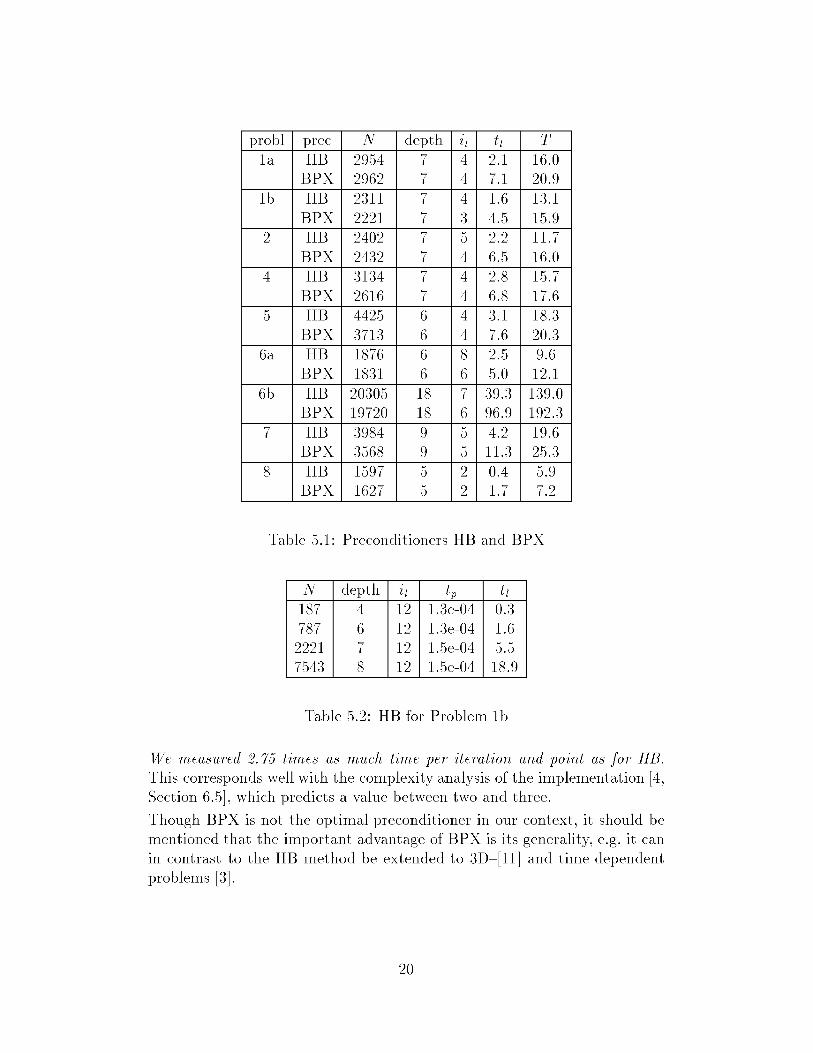
Table 5.1 shows slightly less iteration steps for BPX, an effect which is even more observable for more accurate solutons of the linear y s e m s (f . Tabl 5.2 and 5.3). This corresponds wel with the theory.

However we observe a clear advantage in runtime for HB, which needs less ime in all our test problems without loosng accuracy in the energy norm.

Obviously the higher runtime for BPX is caused by more expensive itera­on steps. Thi s s o w n in detai for Problem lb , see Tables 5.2 and 5.3.

probl re depth HB

BPX 2954 2962

2. 7.

16. 20.

HB BPX

2311 2221

1.6 4.5

13. 15.

HB BPX

2402 2432

2. 6.5

11.7 16.

HB BPX

3134 2616

2.8 6.8

15.7 17.6

HB BPX

4425 13

3. 7.6

18.3 20.3

HB BPX

1876 1831

2.5 5.

9.6 12.

HB BPX

20305 19720

18 18

9. 6.

139. 192.

HB BPX

3984 3568

4.2 11.

19.6 5.3

HB BPX

159 162

0.4 1.7

5. 7.

ble 5.1: P r n d i n e r s HB and BPX

depth H ^ 18 1.e-04 0.3 78 1.3e-04 1.6

2221 1.5e-04 5.5 7543 1.5e-04 18.

able 5.2: HB P r b l

We measured 2.75 times as much time per iteration and point as for HB. This corresponds well with the complexity analysis of the implementation [4, Section 6.5], which predicts a value between two and three.

Though BPX is not the optimal preconditioner in our context, it should be mentioned that the important advantage of BPX is its generality, e.g. it can in contrast t the HB method be extended to 3D-[11] and time dependent

roblems [3]

20

depth H ^ 18 4.e-04 0.6 78 4.0e-04 3.

2221 4.e-04 9.4 7543 4.2e-04 34.

ble 5.3: BPX Pr

5.2 uen of the eratio rror

In this section we tudy once more the aspec of accuracy in the i te ra ton process and present some results i addi ion to hos i Chapter 3.

The multi-level strategy of KASKADE relates the estimated discretization error to the error of the solution of he linear system. It is senseless and not efficient o generate a solution in the iteration process which is more accurate than the discretization. Becaus we do not know the exact errors of the discretization and the iteration, it is necessary t relate both by a afety factor p. It is well chosen if further iterations in the linear solver preconditioned CG-method) have no or only little effect on the accuracy of

the solution on the actual grid. In the first version [13] of KASKADE th authors worked w i h p = 0.25. However, the results from Chapter 3 and from this section uggest that a value of p = 0.01 is safer. ially we recognize an mproved e f e n c y index of the error estimation.

The effect on the runtime by some additional iteration steps is small com­pared with the total time including error e s t i a t o n and integration. Spe­cially in Chapter 3 we saw that the setting of a smaller p on the lower level often improves he convergence h i sory by reachng the requred accuracy on a coarser grid

In some xamples (Tables 5.4 - 5.7) we oted the accuracy to computation with p = 0.25, afterwards we continued the iteration process by choosing smaler values for p and noted the improved accuracy. We counted the ac cumuated number of iterations i. The accuracy is measured in the energy

orm {SL) and a kind of aximum nor grid, see Chapter 1). a le r value of p o fen deceases the maximu error.

21

' -•est £grid

0.50 0.100 0.010 0.001

8.65e-0 7.65e-0 7.36e-0 7.34e-0

9.92e-03 8.04e-03 7.67e-03 7.62e-03

1.81e-0 1.07e-03 8.31e-04 8.15e-04

ble 5.4: Pr a, m e n ) on l v e 5 , N = 301

'-'est £grid

0.50 0.100 0.010 0.001

7 13 15

1.72e-01 1.46e-01 1.29e-01 1.28e-01

1.87e-01 1.55e-01 1.38e-01 1.36e-01

6.67e-02 6.30e-02 9.38e-0 9.33e-0

ble 5.5: Pr 2, (me v e l 5 , N = 47

'-'est £grid

0.250 0.100 0.010 0.001

1.71e-01 1.83e-01 1.87e-01 1.86e-01

3.24e-01 3.00e-01 2.95e-01 2.95e-01

2.43e-01 2.26e-01 2.20e-01 2.19e-01

ble 5.6: P r b l m 6c, ( m e ) o v e l 5 , N 307

5.3 plicit S r s e Form versus L o a l Stiffness a­t r ices

By defaul the KASKADE program does not compute the values of th stiffness matrix explicitly, only the local stiffness matrix of each t r ang l s saved at the orresponding triangle data structure. If the stiffness matrix

is used in the iera t ion process, these local matrices must be added up for every matrix-vector multiplicaton. By special selecion of a parameter in he program here is the possbility to assemble and save the stiffness matrix i sparse form) on each level. Thus we get rid of summing of ocal mat rces

in every matrix multiplication, which accelerates each iteration step. In addition the local stiffness m a t r i e s are not saved in order to reduce th memory equirements. Therefor they must b ecomputed on each level

22

' -•est £grid

0.250 0.100 0.010 0.001

7.57e-01 6.94e-01 6.60e-01 6.58e-01

65e-01 7.09e-01 6.75e-01 6.72e-01

8.01e-02 7.87e-02 7.7e-02 7.7e-02

ble 5.7: Pr , (me v e l 6 , N = 237

even for trangles which have not changed on he latest refinement l v e l

We studied the runtime behavior of KASKADE version (K5) which uses the explicit form of the stiffness matrix. The results are shown in Chapter 3. We ealize that the time of the iteration process (multiplcation with the stiffness

matrix) is shortened but the loss in the integration process (integration is epeated on each level even on triangles which did not change) dominates

the runtime We need about 30% more time than in the version K4 working with local siffness matrices. K5 should be used in cases where the number of ie ra t ion steps is much higher than our test problems.

The complete-matrix verson K5 requires less memory than the saving of all stiffness matrices in K4 (see Chapter 4), but comparedwwith he total amount of memory this advantage eems to be negligible.

hapter

Su

6.1 nalysis of KASKAD

O the test et KASKADE as proved to be a r e l a b l , robust and efc ient a lgorthm.

The refinement trategy based on local extrapolation turns out to be more robust and accurate than the refinement strategy based on the mean value. Further it generates triangulations with far fwer nodes and is s e r i o r i r u n t m e .

The edge oriented error estimator turns out to be e f e n t and accu­rate. In tendency it underestimates the error lightly. On the solution triangulation it agrees with the true error a difference of only

- 7 % xtrapolation t r a t g y used!).

The hierarchical bases preconditioner is as robust and accurat as th BPX preconditioner, but has runtime advantages.

6.2 C o m p r i s o n of KASKAD and PLTM

As a rul of thumb one ay conclude:

KASKADE is 3-5 times faster han PLTMG, but uses 2-3 times as much emory as PLTMG while they ar comparabl robust and reli able.

ore detaied we observed the folowing:

In both programs the near olver needs only about 1 of the total runtime.

The triangle oriented error estimator of PLTMG needs roughly twice as many evaluations per point of the coefficient functions of the elliptic operator as the edge oriented error es imator of KASKADE. This could be a serious drawbac for eal applcations w i h expensive funcion valuations.

Integration process and grid refinement are much faster in KASKADE than in PLTMG for reasons of data ructure and mplementation (C versus F R T R N ) .

24

For the ame reasons PLTMG has he memory advn tage . Th i rad betwen sped and memory requiremen

ppendi Test Prob We use the Dirchlet boundary condition in all examples, except i ampl 6c, where we have addiionally natural boundary c o n d i o n s .

1. The solution of this problem has a harp peak. Two r i a n s of th problem run on different domains.

source equation peak at (0.5,0.117) domain initial triangles angle bounds

solution peak at (0,0 domai

initial t r ianges angle bounds olution

21] Poisson

unit square isosceles right m i m u m 18.43°; maximum 116.57° x(x 1) (y 1 ) e ( ) 2 + ( ) 2 )

h e a g o n with corners (1,0), ( | v 3 / ) , (- i , V / ) , (1,0) , ( i V ) , and (|, - V equilateral minimum 30°; maximum 90° (x + l)(x l ) ( y + l ) ( y 1 ) e (

2. The solution of this ro has a b o u n d r y layer a n g the lnes and y = 1.

source 6, 21, 19] equation V lOOu = / domain uni square initial triangles isosceles right angle bounds minimum 18.43°; m a x i u m 116.57°

h(10x) + cosh(0y) ut

2 cos

3. The solution of this problem has four mild peaks. It is fairly smoo so that a uniform grid should do nearly as wel as adaptive grids. Th equation h nonons tan t coeffiient.

sourc equation domain initial triangles angle bounds olution

21] V (100 + C S 2 X + y)u = /

unit square isosceles right minimum 18.43; m a x i u m 116.5

0.31(5.4 cos 4rx)(m(y y) (5.4 c o s 4 y ) ( ( l + $4) 0.5

= 4(x 0. 4 ( y 0 . 5 )

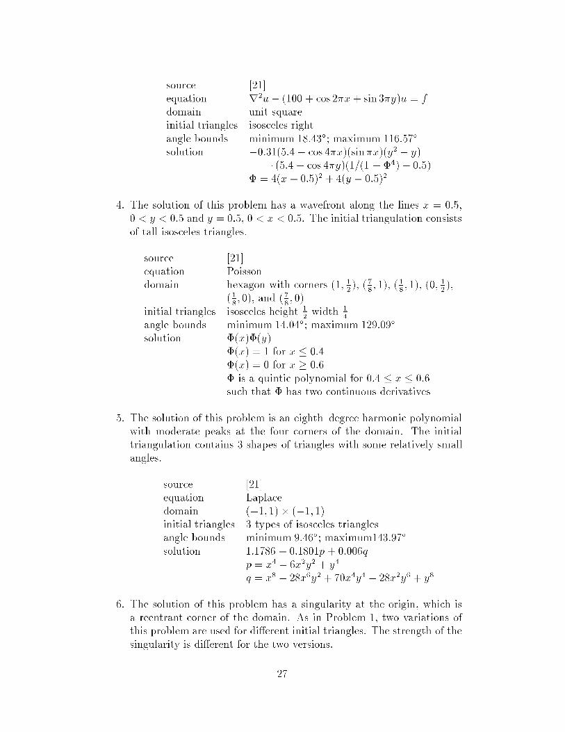
4. The solution of this proble has a wavefront along the lines x = 0.5, 0 < y < 0.5 and y = 0.5, 0 < x < 0.5. The in i ia l t rangulat ion c o n s t s of tall isosceles triangles.

sourc equation domai

initial triangles angl bounds o lu ton

:M (0

21] Poisson hexagon with corners ( | , 0 ) , and ( | , 0 isosceles height | width | m i n m u m 4.04°; maximum 129.09° $ (a )$ (y )

$(x = 1 for x < 0.4 $(x) 0 for x > 0.6 $ is a qu in tc polynomial for 0.4 < x < 0.6 uch that $ has two continuous derivatives

5. The solution of this problem is an eighth-degree harmonic polynomial with moderate peaks at the four corners of the domain. The nitial triangulation contains 3 shapes of trangles with ome relatively al angles.

source equation domain initial triangles angle bounds olution

[21] Laplac ( 1 , 1 ) x ( 1 , 1 ) 3 types of isosceles trangles minimum 9.46°; maximuml43.97° 1 .17860 .1801p + 0.006g

n ? i

p = x ox + y q = x 2Sx + 70x 2Sx + y

6. The solution of this problem has a singularity a the origin, which is a reentrant orner of the domain. As in Problem 1, two variations of this problem are used for different initial triangles. The strength of th ingularity is different for the two versons.

27

sourc equation

a) domai initial triangles angle bounds solution domai

initial triangles angle bounds solution

c) domai

initial triangles angle bounds olution

[2, 7, 8, 19, 20] Laplace L-shaped ( -1 ,1 ) x ( 1 , 1 ) ( 0 , 1 ) x ( 1 , 0 isosceles right minimum 18.43; maximum 116. r2'3 sin ^p (polar coordinates) hexagon as in l with a t along the l n e (y = 0,x > 0) equiateral minimum 30°; maximu 90°

1 4 n v circ wi along the l n e (y = 0,x > equiateral minimum 30°; maximu 90°

1 4 j

. The so lu t i n of this problem is harmonic, but drops very sharply nea (0.01, 0). If the domain were extended to 0, there would e a jump disontinui ty i the boundary condition.

source equation domain initial triangles angle bounds olution

[17] Laplace (0.01,1) x ( 1 , 1 ) right triangles with legs of length 1 and 0.495 minimu 2.43°; maximuml35.29° arctan -

8. The oefficient func t in in the operaor of this equation is discontinu­ous. a(x, y) is piecewise constant with the values 1 and 100 on alternate triangles of the in t ia l triangulation. The olution is contnuous, but the firs derivative as a jump d i s o n t i n u t y where a is discontnuous.

source 6] equation Va'Vu = 0

where a is piecewise constant as d e s c b e d above domain hexagon as in lb initial triangles equiateral angle bounds minimum 30°; maximum 90°

lu y(3x

ppendi : Grid The initial coarse tr ianguation used for al our computation is depicted by slightly thicker pensize in the following drawings. Figures 6.6-6.9 show the meshes for the mean value refnement r a t g y and the extrapolation refine­ment trategy.

igure B . : P b l a, me 275, gr;d 7.73

igure B.2: P r b l b, m e n , 313, id 2.8

igure B.3: P r b l 2, e x t p , 526, gr;d

30

igure B.4: P r o b e m 4, mean, 529, grid 3.

igure B.5: P r o b l m 5, e x t r p , N3 = 253, gr;d 3.37

31

igure B.6: P b l e m 6a, me 32, grid 8.17

igure B.7: Probl a, e x t r a , N 134, £g;d = 9.

32

igure B.8: P r b l b, m e n , 8, id = 4.17

i g u e B.9: P b l b, e x t a p , N7 = 7, egr;d 3.

igure B . 0 : Pr , m e n , 90, grid 6.51

igure B . l : P r b l m 8, e x t , N 535, egid = 114

34

ppend i C o n e n c istor

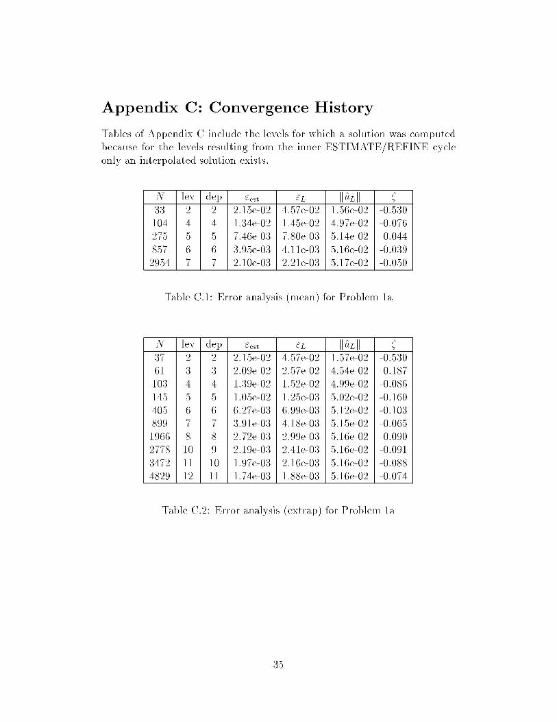
Tables of Appendix C include the levels for which a solution was computed

because for the levels resulting from the inner ESTIMATE/REFINE cyc

only an nterpolated olution xists.

ev dep c-est ÜL 2.15e-02 4.e-02 1.56e-02 0.530

04 1.34e-02 1.45e-02 4.7e-02 0.76

75 46e-03 7.80e-0 5.4e-02 0.044

857 3.95e-03 4.11e-0 5.16e-02 0.039

2954 2.0e-03 2.21e-0 5.17e-02 0.050

bl l: E r r a l y s (me bl

ev dep £-est üL 37 2.15e-02 4.e-02 1.e-02 0.530

61 2.09e-02 2.7e-02 4.54e-02 0.18

1.39e-02 1.52e-02 4.99e-02 0.086

45 1.05e-02 1.25e-0 5.02e-02 0.160

6.7e-03 6.99e-0 5.2e-02 0.03

899 3.91e-03 4.18e-0 5.15e-02 0.065

1966 2.72e-03 2.99e-0 5.16e-02 0.090

78 2.19e-03 2.41e-0 5.16e-02 0.091

3472 11 1.7e-03 2.16e-0 5.16e-02 0.088

4829 11 1.74e-03 1.88e-0 5.16e-02 0.74

ble C 2 : E r r analyss ( x t P r b l

'-•e üL 64

261

051

828

2.86e-02

9.48e-03

4.52e-03

2.00e-03

2.09e-02

8.06e-0

4.11e-0

1.92e-0

4.73e-02

5.11e-02

5.16e-02

5.17e-02

0.368

0.176

0.100

0.04

ble C 3 : E r r analys PLTMG) f Pr

ev dep c-est üL 50 3.51e-01 5.52e-01 1.50e-00 0.364

201 2.26e-01 3.59e-01 1.46e-00 0.70

634 1.53e-01 2.44e-01 1.44e-00 0.73

1672 1.7e-01 1.70e-01 1.44e-00 0.71

4224 52e-02 1.19e-01 1.43e-00 0.368

abl 4: E r r analysis (me P r b l m 6

ev dep est

3.54e-01 5.64e-01 1.50e-00 0.72

51 3.7e-01 4.69e-01 1.48e-00 0.345

62 2.69e-01 4.06e-01 1.46e-00 0.33

81 2.42e-01 3.46e-01 1.45e-00 0.301

94 2.22e-01 3.00e-01 1.44e-00 0.260

2.0e-01 2.86e-01 1.43e-00 0.266

13 2.00e-01 2.52e-01 1.43e-00 0.206

167 1.79e-01 2.24e-01 1.43e-00 0.201

75 13 1.50e-01 1.78e-01 1.43e-00 0.15

467 18 1.13e-01 1.35e-01 1.43e-00 0.163

453 19 13 34e-02 8.7e-02 1.43e-00 0.172

2002 24 17 5.77e-02 6.46e-02 1.43e-00 0. 2670 20 4.99e-02 5.31e-02 1.43e-00 0.060

bl 5: E r r a l y s (ext P r b l m 6