K.N. NINAN*

Economic Liberalization and Rural Poverty Alleviation: The Indian Experience

INTRODUCTION

The economic liberalization process, initiated by India in 1991 following a macroeconomic crisis, has evoked considerable debate and controversy, espe­cially regarding its social implications. Will these reforms, consisting of a Stabilization and Structural Adjustment Programme (SAP), benefit the poor and other marginalized groups by reducing poverty, improving food entitle­ments and access to other basic needs, or will poverty and inequality be accentuated? These questions assume importance especially in the context of a widespread belief that the benefits of reforms have largely accrued to the rich and other better-off sections, with the costs having most often been borne by the poor. Evidence from some recent studies (Gupta, 1992, 1996; Ninan, 2000), suggesting an aggravation of poverty after the reforms, has provided critics with ammunition to point to adverse social effects.

There are several features of India's reforms which raise concern from the perspective of poverty reduction. In the absence of adequate safeguards, the low priority accorded to agriculture under India's SAP (unlike the case of Africa and Latin America), plus the emphasis on reducing public expenditures on the social sector, including food subsidies, as part of the government's deficit-curbing exercises, will hurt the poor and reverse the declining trends in poverty recorded after 1969. The initial endowments and favourable condi­tions, such as a more egalitarian distribution of land and other productive assets allied to human resource development, which facilitated the success of such reforms in East and Southeast Asia, are absent in India. That may well affect the quality and success of the reforms.

Keeping the above in view, the present study seeks to analyse the impact of the economic reforms in India from the perspective of the poor, and poverty reduction. The specific objectives are as follows:

(1) to analyse the trends in poverty in India in the post-reform period as compared with the pre-reform period, both at an all-India level and across states;

*Institute for Social and Economic Change, Bangalore, India.

399

400 K.N. Ninan

(2) to analyse the role of agricultural growth, food prices, access to subsi­dized food, and other factors of rural poverty, at the same levels;

(3) to analyse the trends in (consumption) inequality in India in the pre- and post-reform period; and

(4) to estimate the elasticities of rural poverty in India with respect to se­lected variables, as well as explore factors behind alterations in rural poverty levels in the post-reform period.

DATA AND APPROACH

The data for the analysis are drawn from a report by the World Bank (1997) using its figures on 'Poverty and Growth in India' (Ozler et al., 1996). These have been supplemented by material from official publications of the Govern­ment of India such as the National Accounts Statistics, Estimates of State Domestic Product, Bulletin of Food Statistics and Statistical Abstracts of India. To cover the first objective, the analysis uses the estimates of poverty com­puted by Gaurav Datt (1997), and cited by the World Bank.

The estimates are based on the official poverty line determined by the Planning Commission in 1993. It corresponds to a per capita monthly expendi­ture of 49 Rupees and 57 Rupees for rural and urban areas, respectively, at October 1973-June 1974, measured at 'all-India' prices. These poverty lines correspond to a total household per capita expenditure sufficient to provide, in addition to clothing and transport, a daily intake of 2400 and 2100 calories per person in rural and urban areas, respectively. The poverty line for rural areas was adjusted for subsequent years using the Consumer Price Index for Agricul­tural Labourers (CPIAL) with 1960-61 = 100 and for urban areas, using the Consumer Price Index for Industrial Workers (CPIIW) with 1960 = 100. The poverty estimates by Datt and the World Bank have used a corrected CPIAL series where upward adjustments were made to the nominal price of firewood, which had been kept constant since 1960-61 in the official series. Owing to variations in commodity prices and rates of inflation across states, the official all-India poverty line at 1973-4 prices was adjusted using the state-specific consumer price indices for rural and urban areas to derive the poverty lines by state. These are inflated for subsequent years using the state-specific CPIAL.

There are three estimates of poverty based on the head count ratio (HCR), the poverty gap index (PGI), and the squared poverty gap index (SPGI), which belong to the general class of poverty measures commonly used (World Bank, 1997). They capture the extent, the depth and the severity of poverty. While the HCR indicates the proportion of poor with reference to the specified poverty line, the PGI measures the average distance below the poverty line in the population (counting the non-poor as having a zero poverty gap), expressed as a percentage of the poverty line. The SPGI is based on the individual poverty gaps raised to a power of two; that is, it is the mean of the squared proportion­ate poverty gaps (Ravallion and Datt, 1996a, 1996b; World Bank, 1997).

Poverty estimates are available on an annual basis from the 1950s up to 1973-4 and thereafter, up to 1986-7, on a quinquennial basis. However, with a

Economic Liberalization and Poverty Alleviation 401

view to rebuilding a time series, a decision was taken to revert to an annual basis from 1986-7, using a smaller sample. Despite the deficiencies of the material (such as the uneven spacing and length of the surveys), these are the only series available for such a long time span for any country, and hence have generated wide interest and research on temporal and spatial variations for India.

An earlier study noted that, while rural poverty trends at national and state levels registered a significant increase from 1957-8 to 1968-9, during the subsequent period from 1969-70 to 1986-7 they recorded a marked decline (Ninan, 1994, 1995-6). The rate of decline during the latter period was also higher than the rate of increase in rural poverty during the previous period, both for all India and most states. Hence 1969-70 has been taken as the starting point for analysis over the period up to 1993-4, the latest year for which poverty estimates are available. Although the analysis spans 25 years, we have only 14 observations at all-India level and 12 observations at state level, because of gaps in the data cited earlier. The pre- and post-reform periods are 1969-70 to 1990-91 and 1991-2 to 1993-4.

TRENDS IN POVERTY

For fitting trends the following model is used:

where

g == head-count ratio or poverty gap index or squared poverty gap index, d == dummy variable where d == 0 for the pre-reform period and d == 1 for the

post-reform period, ==time,

d·t ==product of dummy and time variables, u == error term.

From the estimated equations we can derive the equations for the pre- and post-reform periods (period I and period II) as follows:

This model offers advantages in terms of providing greater degrees of free­dom for econometric analysis as inferences about the period-wise trends can be drawn from a single sample rather than two and, more important, it enables us to see whether the slope itself has undergone a change over the two periods. Ordinary least squares (OLS) has been used to estimate the trends in poverty. In the equations where autocorrelation was found to be serious the parameters were re-estimated using the Beach-Mackinnon method. The estimates for the

402 K.N. Ninan

pre- and post-reform periods presented in Tables 1 and 2 are derived from the estimated linear equations using the model for the three alternative measures of poverty.

Table 1 presents the trends in poverty and (consumption) inequality for India. During the pre-reform period from 1969-70 to 1990-91, rural poverty recorded a significant decline in terms of all three indicators, falling at a

TABLE 1 Trends in poverty and inequality (consumption) in India during the pre- and post-reform period from I969-70 to 1993-4

Pre-reform period Post-reform period (1969-70 to 1990-91 (1991-2 to 1993-4)

Poverty indicator Constant Time Constant Time

Rural poverty HCR 59.16* -1.02* 42.32 -0.10 PGI 18.79* -0.46* 6.87 +0.10 SPGI 7.96* -0.23* 1.47 +0.07

Urban poverty HCR 47.79* -0.65* 66.49 -1.36 PGI 14.31* -0.26* 18.65 -0.42 SPGI 5.68* -0.12* 9.45 -0.26

Overall national poverty HCR 56.82* -0.95* 48.99 -0.04 PGI 17.85* -0.42* 9.20 -0.002 SPGI 7.49* -0.20* 3.11 +0.001

Inequality (consumption) Rural Gini 29.91* -0.03 30.26 -0.015 Urban Gini 34.07* +0.05 67.21 -1.23 National Gini 31.06* +0.001 38.56 -0.25

Notes: These equations are derived from the estimated equations using the model mentioned in the text. The trends computed here are linear trends. In the tables in this paper,*,**, and*** indicate coefficients to be statistically significant at I, 5 and 10 per cent levels of significance, respectively. In the equations for the post-reform period derived from the estimated equations, the significance of the constant term is infen-ed on the basis of the statistical significance of the dummy variable in the estimated equation, while that of the time trend variable is infen-ed on the basis of the statistical significance of the (d.t) variable.

Source: The basic data for the above analysis have been taken from World Bank (1997). The estimates of poverty using different indicators of poverty, and Gini ratios reported therein, have been computed by Gaurav Datt.

Economic Liberalization and Poverty Alleviation 403

sharper rate than urban poverty. In contrast, the post-reform period from 1991-2 to 1993-4 recorded either a notable weakening of the negative trend in the head count ratio, or a reversal on the basis of PGI and SPGI, which measure the depth and severity of poverty. Urban poverty in terms of all indicators continued to record declining trends (though none were statistically signifi­cant). Trends in consumption inequality for rural India recorded a decline during both periods, whereas in respect of urban areas this trend was positive during the pre-reform period and negative in the latter period, but none were statistically significant.

Trends in rural poverty for 15 major states appear in Table 2. It is interesting to see that in the pre-reform period all 15 recorded a significant decline in poverty levels, in terms of all three indicators, but during the post-reform period there is a diversity of patterns. Eleven states continued to record nega­tive trends in rural poverty for one or more poverty indicators, although these negative trends were not statistically significant in most cases. Only Gujarat and Kamataka continued to record significant declines in rural poverty levels across the three poverty indicators, and that, too, at a faster pace.

The intensification of rural diversification in Gujarat and Kamataka may explain the sharper decline in rural poverty levels in the post-reform period. Madhya Pradesh, Tamil N adu and Assam recorded a significant decline in terms of HCR or SPGI. Four states report a reversal with the rural poverty trends changing from negative to positive, although these trends were not statistically significant. Of them, Orissa and West Bengal fall in the eastern belt of India where poverty appears endemic. But most surprising is that Punjab and Haryana, which had been in the forefront in ushering in the 'Green Revolution' in India, and where poverty levels recorded a significant decline earlier, report a positive trend (although not statistically significant) in terms of all three poverty indicators. The rate of increase in rural poverty levels for Haryana is also quite sharp. For instance, the HCR for Haryana which was 20.72 during 1990-91, rose to 21.73 in 1992 and 33.08 in 1993-4 during the post-reform period. Similarly, the PGI rose from 4.95 to 4.98 and 7.64 respec­tively; and the SPGI from 1.596 to 1.538 and 2.531, respectively. Sharp hikes in procurement and issue prices of food grains during the post-reform period in response to the pressures of the farmers' lobby appear to have worked to the detriment of the rural poor in the traditional green revolution belt of the country.

FACTORS AFFECTING RURAL POVERTY

Given that agriculture contributes more than a third of India's gross national product (GNP) and supports over two-thirds of the population, it is obvious that the fortunes of the rural poor are intrinsically linked to those of farming. Ahluwalia ( 1978, 1985) observed a close negative association between the incidence of rural poverty in India and agricultural performance. The impact occurs in several ways. Higher agricultural output helps reduce prices as well as improve food availability, both of which favour the poor. It will generate

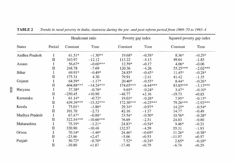
TABLE2 Trends in rural poverty in India, statewise during the pre- and post-reform period from 1969-70 to 1993--4

Headcount ratio Poverty gap index Squared poverty gap index

States Period Constant Time Constant Time Constant Time

Andhra Pradesh I 61.51 * -1.30** 19.68* -0.58* 8.36* -0.29* II 343.97 -12.12 113.22 -4.13 49.64 -1.85

Assam I 56.67* -0.60*** 12.59* -0.17 4.06* -0.06 II 248.78 -7.69 120.36 -4.26 55.25*** -2.02***

Bihar I 69.91 * -0.49* 24.85* -0.45* 11.45* -0.28* II 175.31 4.30 79.91 -2.41 41.42 -1.35

Gujarat I 64.59* -1.17* 20.40* -0.55* 8.44* -0.26* II 404.88*** -14.24*** 174.65*** -6.44*** 83.85*** -3.13***

.i:. Haryana I 37.38* -0.76* 9.65* -0.24* 3.47* -0.10* 0

.i:. II -250.45 +10.90 -48.77 +2.16 -19.73 +0.85

Karnataka I 61.14* -0.72* 19.03* -0.28* 7.95* -0.13* II 439.39*** -15.32*** 172.30*** -6.25*** 79.26*** -2.92***

Kerala I 75.01 * -1.86* 29.34* -0.97* 14.25* -0.54* II 101.70 -2.73 42.16 -1.37 14.77 -0.49

Madhya Pradesh I 67.47* -0.88* 23.54* -0.50* 10.'i6* -0.28* II 322.54*** -10.66*** 76.69 -2.51 24.83 -0.80

Maharashtra I 75.19* -1.21* 24.83* -0.54* 9.46* -0.21 II 320.90 -10.48 132.57 -4.59 55.31 -1.93

Orissa I 70.14* -1.40* 24.46* -0.69* 11.26* -0.38* II -23.86 +2.47 -5.06 +0.53 -11.97 +0.57

Punjab I 30.72* -0.70* 7.52* -0.24* 2.65* -0.10* II -30.80 +l.87 -17.48 +0.79 -6.74 +0.29

Rajasthan I 67.40* -1.16* 23.74* -0.52* 10.88* -0.27** II 143.32 -3.53 61.11 -1.90 31.17 -1.04

Tamil Nadu I 67.54* 1.09* 22.28* -0.48* 9.67* -0.24* II 294.40*** -9.91 *** 119.56 -4.27 52.11 -1.89

U ttar Pradesh I 54.62* -0.84* 15.19* -0.30* 5.72* -0.13* II 196.49 -5.97 98.68 -3.42 55.17 -2.00

West Bengal I 66.56* -1.49* 21.42* -0.62* 9.08* -0.30* II 50.15 -0.88 10.34 -0.22 -0.27 +0.06

Notes: I, 1969-70 to 1990-91; II, 1991-2 to 1993-4. See also notes to Table 1.

Source: As for Table 1.

~ 0 Ul

406 K.N. Ninan

employment opportunities on the land and spur growth in the non-agricultural sector, thereby creating income-earning opportunities. Agricultural growth on the whole will give a fillip to overall economic development. However, if it involves a shift from labour-intensive crops and technologies to labour-saving ones, this could work to the detriment of the rural poor, since agricultural wages constitute a major component of their incomes. Evidence from India, however, suggests that on balance the green revolution resulted in increased labour use and real wage rates (Dantwala, 1985).

Nevertheless, some argue that, in the context of the institutional and struc­tural constraints characteristic of most low-income countries, the beneficial effects of growth can be mostly expropriated by the non-poor. The trickle­down effect implied by Ahluwalia's finding of a negative correlation between agricultural growth and the incidence of rural poverty was thus challenged by a number of researchers (Rajaraman, 1975: Griffin and Ghose, 1979). However, these observations are based on flimsy theoretical or empirical support. For instance, Rajaraman's findings implying a weak causal link between agricul­tural growth and rural poverty were based on just ten observations, of which only four were in the post-green revolution period. In specifying variables it was decided to use agricultural output expressed on a per capita basis, rather than on the per acre basis as in Datt and Ravallion (1998), who argued that, although output on a per person and per acre basis are highly correlated (the coefficient being 0.89 over 35 annual observations), for predictive purposes output expressed on a per acre basis is more appropriate for use in poverty equations. The reason is that, in a country like India, rapid population growth can negate the favourable impact of an improvement in crop yields on poverty levels.

Poverty is affected by inflation, which acts like a regressive tax on the poor, leading to a deterioration in their entitlements and real incomes (Sen, 1981). Since food constitutes the predominant portion of the consumption basket of the poor, rising food prices cause great anxiety. Even subsistence farmers who are net purchasers of foodgrains can be affected (Mellor and Desai, 1985; Ninan, 1994, 1995-6).

Population growth, poverty and the environment are closely interlinked. Rapid population growth affects poverty in many ways. It can offset the benefi­cial effects of economic growth on poverty as experienced by some South Asian countries. Moreover, poverty intertwined with rapid population growth exercises intense pressure on scarce environmental resources, resulting in envi­ronmental degradation through overexploitation of fragile resources.

Particularly since 1969, there have been a number of institutionalized wel­fare programmes aimed at poverty relief. Of these the provision of subsidized food through the public distribution system (PDS) has assumed great signifi­cance. However, except in some states in southern India, the programme is largely urban-oriented, although in the recent past improvements have been made to extend its reach to rural areas elsewhere and to improve selectivity. Time-series data are available only in the form of PDS offtake of foodgrains aggregated for rural and urban areas, as well as the number of fair price shops (available separately for rural and urban areas). These limitations have been

Economic Liberalization and Poverty Alleviation 407

kept in view while specifying the PDS variable. The role of other factors, such as inequality in rural consumption (which is a proxy for income inequality) and infrastructure development, are also examined.

It has been customary to include a time trend variable in poverty functions to serve as a cover-all variable for all other time-related factors influencing pov­erty not explicitly considered in a given model. This implicitly assumes that all time-related factors exercise unidirectional influences on poverty, which is questionable. The inclusion of a separate time trend variable in these circum­stances is, therefore, questionable and could even affect the estimates of other explanatory variables.

Bearing these factors and data limitations in mind, the causal factors behind rural poverty in India between 1969-70 and 1993-4 can be examined. A time­series analysis at all-India level, and a cross-section analysis of inter-state data at two points of time, 1987-8 and 1993-4, which belong to the pre- and post­reform periods, respectively, are used. The variables are as a dependent variable (HCR, PGI or SPGI - all in percentages) and independent variables. To study the impact of agricultural growth (or performance), food prices, rural popula­tion pressure on environmental resources, access to subsidized food through the PDS, inequality in rural consumption levels, and infrastructure develop­ment on rural poverty levels, the following variables are considered.

( 1) Agricultural output/performance variables (three specifications): NDPAGRI - real net domestic product (NDP) from agriculture at 1960-61 prices per rural inhabitant, NDPPRM - real NDP from the primary sector (excluding mining and quarrying) at 1960-61 prices per rural inhabitant, SDPAGRI - state domestic product from agriculture per state rural inhabitant.

(2) Price variables (two specifications): FDPR - consumer price index for agricultural labourers for food items (where 1960-61=100) for rural areas, RELFDPR - relative food to general consumer price index for agricul­tural labourers ( 1960-61=100) for rural areas.

(3) Population pressure on environmental resources: RPPAL - rural population pressure on agricultural land expressed in 100 000 people per ha. of gross cropped area (so as to take note of land-augmenting technologies which became prominent after the green revolution).

(4) Institutional intervention (PDS): PDS - proportion of PDS offtake of foodgrains to total net availability of foodgrains, PDSFP - number of fair price shops per 100 000 people (for rural areas).

(5) Consumption inequality: INEQUAL - inequality in rural consumption (Gini ratios).

(6) Infrastructure development: INFRADEV - infrastructure development index as constructed by the Centre for Monitoring the Indian Economy, Bombay.

408 K.N. Ninan

Not all these variables have been included in an equation because of the constraints of limited observations. Further, while some variables were com­mon to both the time series and cross-section analyses, others were included in only one of them.

The agricultural, as well as price, variables were also used in their lagged forms. One could argue that the level of poverty in a given year is determined not only by that year's agricultural performance but also by that of the previous year. A good crop enables a poor household not only to repay past debts but also to build up reserves to meet unforeseen circumstances. Similarly, inflation has a lagged effect. For instance, given the low incomes of the poor, a steep rise in the prices of essential commodities may force them to borrow in order to arrest a deterioration in their consumption, the after-effects of which will be felt in subsequent years as well. To take note of these lagged effects, an alternative specification of the output and price variables is used which is computed at { t + (t - 1)} I 2.

Multiple linear regression using OLS was used to estimate the coefficients. In those equations where the Durbin-Watson statistic indicated serious prob­lems of autocorrelation, the parameters were re-estimated using the Beach-Mackinnon method. The INFRADEV variable was found to be strongly correlated with the '}gricultural output variable in some equations, and hence dropped. Only those equations which gave meaningful results have been repre­sented below.

Table 3, which presents the results time series analysis for all India, indi­cates that, while the agricultural output and PDS variables are negatively correlated with the incidence of rural poverty measured in terms of all the three indicators, the relative food price variable has a positive effect. The coeffi­cients are statistically significant in most cases. The Gini variable which measures inequality in rural consumption (a proxy for income inequality) is also positively correlated with the incidence of rural poverty, although the coefficient is not statistically significant. These observations are also valid for the equations where we have used the lagged versions of the agricultural performance and relative food price variables. The R-squared values are very high. These variables are able to explain between 88 to 97 per cent of the variation in the incidence of Indian rural poverty.

Results of the cross-section analysis of the factors affecting the inter-state incidence of rural poverty for two points of time, 1987-8 and 1993-4 (pre­and post-reform, respectively), are presented in Table 4. Here again, while the agricultural performance and PDS variables are negatively correlated with the incidence of rural poverty across states, the food price, Gini and RPPAL variables are positively associated with poverty levels. The infra­structure development index variable is negatively correlated with incidence. The agricultural performance variable is statistically significant in most of the estimated equations. Although the other variables had the expected signs, none of them were statistically significant. In fact, the addition of the other variables even resulted in the agricultural performance coefficient becoming statistically not significant in some equations, which partly reflects the few degrees of freedom available for the analysis. An earlier study had estab-

TABLE3 Determinants of rural poverty in India I969-70 to I993-4

Equation No. Estimated linear equations R2 DW Statistic Rho

Dependent variable: head count ratio (per cent) 1 -82.33-0.34 NDPAGRI* + 2.01 RELFDPR** - 2.13 PDS* 0.92 1.99 -0.74** 2 123.26* - 0.33 NDPAGRI* - 2.00 PDS* + 0.37 GINI 0.88 1.94 -0.58 3 -79.39- 0.28 NDPPRM* + 1.89 RELFDPR** -1.94 PDS* 0.94 1.80 0.77** 4 124.44* - 0.28 NDPPRM* - 1.72 PDS* + 0.01 GINI 0.90 1.91 0.53 5 -5.11 - 0.38 LNDPAGRI* + 1.21 LRELFDPR - 0.63 PDS 0.91 1.91 0.48 6 -105.85 -0.31LNDPPRM*+2.08 LRELFDPR- 1.10 PDS** 0.89 1.59

Dependent variable: poverty gap index 7 -22.15 - 0.16 NDPAGRI* + 0.71 RELFDPR*** - 0.93 PDS* 0.94 2.12 -0.78**

+>- 8 53.34* - 0.16 NDPAGRI* - 0.87 PDS* + 0.03 GINI 0.91 2.05 -0.65** 0 \0 9 -21.07 -0.13 NDPPRM* + 0.65 RELFDPR** - 0.84 PDS* 0.97 1.96 -0.87*

10 -33.91- 0.17 LNDPAGRI* + 0.79 LRELFDPR- 0.50 PDS** 0.91 1.72 11 -33.89* - 0.14 LNDPPRM* + 0.75 LRELFDPR- 0.47 PDS** 0.91 1.68

Dependent variable: squared poverty gap index 12 -7.03 - 0.08 NDPAGRI* + 0.30 RELFDPR* - 0.45 PDS* 0.95 2.13 -0.77** 13 -6.43 -0.07 NDPPRM* + 0.27 RELFDPR** - 0.41 PDS* 0.97 1.94 -0.86* 14 -12.53 - 0.09 LNDPAGRI* + 0.34 LRELFDPR- 0.25 PDS** 0.91 1.67 15 -12.53 - 0.07 LNDPPRM* + 0.32 LRELFDPR- 0.23 PDS** 0.91 1.61

Notes: For a description of the independent variables refer to the text. Variables prefixed by the letter 'L' are lagged variables. Only the agricultural performance and price variables have been used in the lagged form in some equations. For *, ** and ***, refer to notes in Table 1.

Source: Table I; also official documents such as the Bulletin of Food Statistics, Statistical Abstracts of India, Govt. of India.

..,. ,_. 0

TABLE4 1993-4

Determinants of the inter-state incidence of rural poverty in India: a cross-section analysis for 1987-8 and

Equation No. Estimated linear equations

1 2 3

4 5 6

7 8 9

10 11

12 13 14

15 16

Notes:

1987-8 Dependent variable: head count ratio (per cent) 28.48 - 0.01 SDPA ** + 0.03 FDPR - 2.91 PDSFP + 0.11 GINI -49.34-0.01SDPA**+1.00 RELFDPR-4.36 PDSFP + 0.13 GINI -47.79 - 0.004 SDPA + 0.96 RELFDPR - 3.58 PDSFP + 0.46 GINI - 0.10 INFRADEV

Dependent variable: poverty gap index -1.01 -0.002 SDPA** + 0.01FDPR-1.97 PDSFP + 0.26 GINI -32.62 - 0.002 SDPA ** + 0.40 RELFDPR - 2.56 PDSFP + 0.27 GINI -32.03 - 0.001 SDPA + 0.39 RELFDPR - 2.26 PDSFP + 0.39 GINI - 0.04 INFRADEV

Dependent variable: squared poverty gap index -2.63 -0.001SDPA*+0.005 FDPR- 1.04 PDSFP + 0.15 GINI -17.99-0.001SDPA**+0.19 RELFDPR-1.34 PDSFP + 0.16 GINI -17.71 - 0.0004 SDPA + 0.18 RELFDPR- 1.19 PDSFP + 0.22 GINI - 0.02 INFRADEV

1993-4 Dependent variable: head count ratio (per cent) -106.10 - 0.003 SDPA * + 1.54 RELFDPR - 3.69 PDSFP -72.64- 0.001SDPA+1.33 RELFDPR- 0.20 INFRADEV + 0.70 RPPAL

Dependent variable: poverty gap index -33.57 - 0.001 SDPA ** + 0.46 RELFDPR - 3.92 PDSFP -30.21 - 0.001 SDPA ** + 0.40 RELFDPR + 0.04 GINI -23.43 - 0.0002 SDPA + 0.39 RELFDPR - 2.49 PDSFP - 0.05 INFRADEV + 0.17 RPPAL

Dependent variable: squared poverty gap index -13.29 - 0.0003 SDPA*** + 0.17 RELFDPR - 1.93 PDSFP + 0.12 GINI -16.16- 0.00004 SDPA + 0.19 RELFDPR-0.43 PDSFP + 0.14 GINI-0.03 INFRADEV + 0.12 RPPAL

See Tables 1 and 3.

R2 OW statistic

0.56 1.95 0.57 2.09 0.62 1.92

0.51 1.89 0.52 2.04 0.58 1.79

0.46 1.85 0.49 2.00 0.57 1.69

0.46 2.38 0.59 2.01

0.37 2.42 0.33 2.58 0.47 2.18

0.33 2.37 0.45 1.90

Economic Liberalization and Poverty Alleviation 411

lished these variables as having a significant influence on the inter-state incidence of rural poverty in India (Ninan, 1994; 1995-6). The estimated equations are able to explain 33 to 62 per cent of the variations in the inter­state incidence of rural poverty.

ELASTICITIES OF RURAL POVERTY

The elasticities of rural poverty levels in India with respect to selected vari­ables during the period under review show that a 1 per cent rise in the per capita real NDP from agriculture reduced rural poverty levels in India by over 1.4 per cent in terms of the HCR and still higher, by 2.5 to 3.4 per cent, in terms of the PGI and SPGI (Ninan, 2000). Similarly, a 1 per cent rise in the offtake of PDS foodgrains reduced rural poverty levels by 0.5 to 0.9 per cent across the three poverty indicators. A 1 per cent rise in the relative prices of food, however, led to a sharp rise in poverty levels, ranging from 5.3 to over 6.5 per cent across the three poverty indicators. The increase in poverty levels following a rise in relative food prices was sharper in the case of rural poverty as compared to urban poverty (ibid.). Similarly, an incre,ase in the offtake of PDS foodgrains brought about a sharper reduction in rural poverty as com­pared with that in urban areas (ibid.).

The elasticities of inter-state incidence of rural poverty during 1987-8 (pre­reform) and 1993-4 (post-reform,) revealed that a 1 per cent rise in the per capita state domestic product (SDP) from agriculture and access to PDS re­duced inter-state incidence by about 0.5 to 0.8 per cent and 0.03 to 0.3 per cent, respectively, during 1987-8 and 1993-4 across the three poverty indica­tors. The poverty-alleviating role of agricultural growth and access to PDS was sharper in terms of PGI and SPGI. A 1 per cent rise in relative food prices led to a more than proportionate rise in inter-state poverty incidence. But most interesting was that, while in 1987-8 this increase ranged between 1.04 to 1.4 per cent across the three poverty indicators, during 1993-4, after reform, this increase was sharper, ranging from over 2.6 to 3.2 per cent in terms of the three poverty indicators. The poverty-aggravating effect of a rise in relative food prices on rural poverty is more prominent in the post-reform period as com­pared with pre-reform years.

RESULTS OF STEPWISE REGRESSIONS

To find out the relative contribution of selected variables to variations in rural poverty levels in India during 1969-70 to 1993-4, stepwise regressions were computed. The R-squared values of these estimated equations, which shed light on the contribution of these variables to poverty, indicated that over 90 per cent of the variation in rural poverty levels in India was explained by NDPAGRI, RELFDPR and PDS (Ninan, 2000). The agricultural performance variable alone was able to explain about 79 to 86 per cent of the variation. The addition of a relative food price variable resulted in a 2 to 3 per cent improve-

412 K.N. Ninan

ment in the explanatory power of the estimated equations, while inclusion of the PDS variable further raised R-squared values by 5 to 9 per cent (ibid.).

The above, however, does not tell us what factors may have contributed to a worsening of poverty in India in the post-reform period. To investigate this, stepwise regressions were run to examine the contribution of selected variables to variations in the inter-state incidence of rural poverty. Although 1990-91, as the year on the eve of the reforms, would have been ideal to compare the situations, the poverty estimates for that year are based on a thin sample, unlike those for 1987-8 and 1993-4. The variables considered were SDPAGRI (per capita state domestic product from agriculture), RELFDPR (relative food price) and PDSFP (number of fair price shops per 100 000 population for state rural areas). The results indicated that, during 1987-8, 30 to 52 per cent of the variations in the inter-state incidence of rural poverty are accounted for by SDPAGRI alone (ibid.). These proportions were lower during 1993-4, ranging from 21to33 per cent. Most noteworthy, however, was that, when the RELFDPR variable was also included, the explanatory power of the estimated equations which recorded only a marginal improvement of 2 to 3 per cent during the pre­reform year, 1987-8, rose substantially, by 5 to 12 per cent, during the post-reform year, 1993-4. The role of food prices in affecting the inter-state incidence of rural poverty appears to be greater in the post-reform year as compared to the pre-reform year. The addition of PDSFP led to only a slight improvement in the R-squared values of the estimated equation for rural pov­erty in respect of two poverty indicators, HCR and PGI. But in respect of SPGI the value rose further, by 8 and 9 per cent, in 1987-8 and 1993-4, respectively (ibid.). While acknowledging a deterioration of rural poverty in India in the immediate year or two after the reforms, some have argued that a poor crop harvest was responsible for this. A close examination of the data, however, reveals that the per capita real NDP from agriculture during the post-reform period was conspicuously higher than during most years from 1969-70 to 1987-8 in the pre-reform period, as stated earlier (ibid.). Other factors may, therefore, account for the deterioration in rural poverty levels in the post­reform period.

RURAL POVERTY TRENDS UNDER WITH AND WITHOUT REFORM SCENARIOS

A general criticism of most studies that have assessed the social implications of such reforms in India, and elsewhere, is that they fail to provide a counter­factual analysis. In other words, what would the trends in poverty have been in the absence of the reforms? However, data inadequacies preclude us from attempting such a rigorous analysis except in the cases of Punjab and Haryana, under a with and without reform scenario. Using the model spelt out earlier, it was noted that, while rural poverty trends in both states recorded significant declines across the three poverty indicators in the pre-reform period, during the post-reform period these trends reported a reversal, though not to a statistically significant extent (Table 5). In the alternative case, under a without reform

Economic Liberalization and Poverty Alleviation 413

TABLE 5 Rural poverty trends in Haryana and Punjab under with and without reform scenarios during 1969-70 to 1993-4

With reform scenario Without reform scenario

State and Pre-reform Post-reform Overall period poverty indicators period period

Haryana Head count ratio -0.76* +10.90 -0.55* Poverty gap index -0.24* +2.16 -0.18* Squared poverty gap index -0.10* +0.85 -0.07*

Punjab Head count ratio -0.70* +l.87 -0.62* Poverty gap index -0.24* +0.79 -0.22* Squared poverty gap index -0.10* +0.29 -0.09*

Notes: I. Pre- and post-reform periods, 1969-70 to 1990-91 and 1991-2 to 1993-4, respectively; overall period, 1969-70 to 1993--4. 2. Trends computed here are linear trends. 3. * Statistically significant at 1 per cent level of significance. 4. In the equations for the with reform scenario, trends have been com­puted using the model explained in the text wherein a dummy variable is included to account for the pre- and post-reform period as indicated in the text. In the without reform scenario, trends have been computed for the period from 1969-70 to 1993--4, omitting the dummy variable; in other word, the trends are computed assuming a without reform scenario. Under this alternative case we have only one equation for the whole period.

scenario, trends have been fitted by omitting the dummy variable for the period 1969-70 to 1993-4. As is evident, under that scenario, rural poverty trends recorded a significant decline in terms of all three poverty indicators. Thus, as stated earlier, rural poverty in Punjab and Haryana seems to have been aggra­vated in the post-reform period.

CONCLUSIONS

Evidence presented here suggests that, while rural, urban and overall national poverty levels in India recorded a significant decline during the pre-reform period from 1969-70 to 1990-91, during the post-reform period from 1991-2 to 1993-4 these negative trends have weakened or even become reversed in terms of one or more of the three poverty indicators. While rural poverty levels in terms of HCR continued to record negative trends in the post-reform period, in terms of PGI and SPGI a reversal is reported, with the trends changing from negative to positive, although these are not statistically significant. Across

414 K.N. Ninan

states there is a diversity of trends and patterns. While during the pre-reform period all the 15 states recorded significant reductions in rural poverty levels in terms of all the three poverty indicators, during the post-reform period the scenario has changed. Only Gujarat and Karnataka continued to record signifi­cant declines in rural poverty - indeed, at a faster rate. Four states reported a reversal of fortunes with the negative trends turning positive during the post­reform period in terms of one or more poverty indicators. These include Orissa and West Bengal (in SPGI only) which fall within the eastern belt of the country known for its endemic poverty. But most surprising is that Punjab and Haryana, the two states which ushered in the green revolution in India and where rural poverty levels had recorded significant reductions earlier, have reported a reversal of fortunes.

The study also confirmed the strong negative association between agricul­tural growth, access to PDS and rural poverty levels in India, whereas relative food prices and inequality in rural consumption were positively associated with rural poverty levels. These were valid for all three poverty indicators. The infrastructure development index was negatively associated with the inter-state incidence of rural poverty in India, whereas rural population pressure on agri­cultural lands was positively associated.

The increase in poverty levels following a rise in food prices is sharper in the case of rural poverty, while the poverty-aggravating effect appears to be greater during the post-reform period. Whether the reforms per se are to be blamed for this, as opposed to the choice of inappropriate policies during the reform period (for example, the government's policy in effecting sharp hikes in procurement prices, and issue prices of PDS foodgrains) is a matter to be debated.

There is no doubt that rapid economic growth is essential for bringing about a significant reduction in poverty levels in India. But it is not only growth per se but also the pattern of growth that matters. Policies to promote agricultural growth, improve access to the PDS and infrastructure development, along with measures to control inflation, population growth and reducing inequalities, hold the key to making a dent in poverty in India and need to be taken note of in implementing reforms.

BIBLIOGRAPHY

Ahluwalia, M.S. (1978), 'Rural Poverty and Agricultural Performance in India', Journal of Development Studies, 14, 298-323.

Ahluwalia, M.S. (1985), 'Rural Poverty, Agricultural Production and Prices: A Re-Examination', in J.W. Mellor and G.M. Desai (eds), Agricultural Growth and Rural Poverty- Variations on a Theme by Dharm Narian, Baltimore, MD: Johns Hopkins University Press.

Dantwala, M.L. (1985), 'Technology, Growth and Equity in Agriculture', in J.W. Mellor and G.M. Desai (eds), Agricultural Growth and Rural Poverty- Variations on a Theme by Dharm Narian, Baltimore, MD: Johns Hopkins University Press.

Datt, G. (1997), 'Poverty in India 1951-1994-Trends and Decomposition', IFPRI, Washington, DC (mimeo).

Datt, G. and Ravallion, M. (1997), 'Macroeconomic Crisis and Poverty Monitoring: A Case Study for India', Review of Development Economics, 1, 135-52.

Economic Liberalization and Poverty Alleviation 415

Datt, G. and Ravallion, M. (1998), 'Farm Productivity and Rural Poverty in India', Journal of Development Studies, 34, 62-85.

Griffin, K.B. and Ghose, A.K. ( 1979), 'Growth and Impoverishment in the Rural Areas of Asia', World Development, 7, 361-83.

Gupta, S.P. (1992), 'Economic Reform and Its Impact on the Poor', Economic and Political Weekly, 30, 1295-313.

Gupta, S.P. (1996), 'Recent Economic Reforms in India and Their Impact on the Poor and Vulnerable Sections of Society', in C.H.H. Rao and H. Linnemann (eds), Economic Reforms and Poverty Alleviation in India, lndo-Dutch Studies in Development Alternatives Series no 17, New Delhi: Sage.

Lipton, M. and Ravallion, M. (1995), 'Poverty and Policy', in J. Behrman and T.N. Srinivasan (eds), Handbook of Development Economics, vol. III, Amsterdam: Elsevier.

Mellor, J.W. and Desai, G.M. (eds) (1985), Agricultural Growth and Rural Poverty - Variations on a Theme by Dharm Narian, Baltimore, MD: Johns Hopkins University Press.

Ninan, K.N. ( 1994), 'Poverty and Income Distribution in India', Economic and Political Weekly, 24, 1544-51.

Ninan, K.N. (1995-6), 'Agricultural Growth, Institutional Intervention and Rural Poverty Trends - Their Linkages in the Context of Structural Adjustment and Economic Liberalisation in India', Regional Development Studies, Winter, vol. II, United Nations Centre for Regional Development, Nagoya, Japan.

Ninan, K.N. (2000), Economic Reforms in India - Impact on the Poor and Poverty Reduction, IDS Working Paper no. 102, Brighton: Institute of Development Studies.

Ozier, B., Datt, G. and Ravallion, M. (1996), A Data Base on Poverty and Growth in India, Washington, DC: World Bank, Policy Research Department.

Rajaraman, I. (1975), 'Poverty, Inequality and Economic Growth: Rural Punjab - 1960-61 to 1970-71 ',Journal of Development Studies, 11, 278-90.

Ravallion, M. and Datt, G. (1996a), India's Chequered History in the Fight Against Poverty: Are There Lessons for the Future?, Washington, DC: World Bank, Policy Research Department.

Ravallion, M. and Datt, G. (1996b), Growth, Wages and Poverty-Time Series Evidence for Rural India, Washington, DC: World Bank, Policy Research Department.

Sen, A. (1981), Poverty and Famines: An Essay on Entitlements and Deprivation, New Delhi: Oxford University Press.

Tendulkar, S.D. and Jain, L.R. (1995), 'Economic Reforms and Poverty', Economic and Political Weekly, 30, 1373-8.

World Bank (1997), India: Achievements and Challenges in Reducing Poverty, report no. 16483-IN, Washington, DC: World Bank.