kinetics simple models

Kinetics: Simple Models © K. J. Kearfott

Kinetics: Differential Equations and Simple Compartmental Models

K. J. KearfottDepartment of Nuclear Engineering

and Radiological SciencesCollege of EngineeringUniversity of Michigan

Ann Arbor, MI48109-2104

(734) 763-9117FAX (734) [email protected]

Suggested ReadingCember: Chapter 4, pp. 195-196, pp. 299-308, pp. 315-320, pp. 550-554 Evans: Chapter 15Krane: Sections 6.3-6.6Lamarsh: Section 2.9Moe: Chapter 2Shleien: p. 3-14, 3-16 to 3-17, 12-7, 12-12 to 12-22Turner: Section 3.12

Suggested ReviewKJK lectures: Activity and the Decay Law

Sunday, September 11, 2011


Outline• Differential equations and compartmental models

• Simple cases of decay Pure decay Multiple loss terms (leaking tank) Decayed atoms as a compartment Decayed atoms as a compartment with multiple ! loss terms

• Production with decay General case of production with decay Different production terms Decayed atoms for production with decay Production with multiple loss terms Decayed atoms for production with multiple loss ! terms

• Maximums and steady states Maximum activity produced Steady state Atmospheric 14C Radiocarbon dating Production with gas mixing in a room

• Activation Simple activation Activation with burnup



Differential Equation of Importance to HP

• Most differential equations used in radiation protection are of general first order linear form

• In fact, the most common differential equation is the simplest form of Bernoulli’s equation (n = 1)

• Once solved, the solution may be remembered and applied to almost all situations



Important DE, Cont’d.Differential equation to be solveddy x( )dx

+ p(x)y x( ) = q(x)

Solution

y(x) = e! p( x)dx" e

+ p( x )dx"" q(x)dx + C# $ %

& ' (

wherex : independent variabley(x) : dependent variablep(x) : function of x (no explicit y - dependence), uniqueto the equation of interestq(x) : function of x (no explicit y - dependence), uniqueto the equation of interestC : constant of integration, determined from boundaryconditions (e.g. initial conditions)


dy x( )

dx+ p(x)y x( ) = q(x) -(1)

Multiply by ep(x )dx! , the "integrating factor" for

this case

ep(x )dx! dy x( )

dx+ e

p(x )dx! p(x)y x( ) = ep(x )dx! q(x) -(2)

Note that

(xy)'=x'y+y'x, thus

d ep(x )dx! y x( )"

#$%&'= e

p(x )dx! dy x( )

dx+ e

p(x )dx! d p(x)dx!( )y x( )

d ep(x )dx! y x( )"

#$%&'= e

p(x )dx! dy x( )

dx+ e

p(x )dx! p(x)y x( )

ep(x )dx! dy x( )

dx= d e

p(x )dx! y x( )"#$

%&'( e

p(x )dx! p(x)y x( ) -(3)

Putting (3) in (2), and simplifying

d ep(x )dx! y x( )"

#$%&'( e

p(x )dx! p(x)y x( ) + ep(x )dx! p(x)y x( ) = e

p(x )dx! q(x)

d ep(x )dx! y x( )"

#$%&'= e

p(x )dx! q(x) -(4)

Integrate both sides of (4), and simplifying

d ep(x )dx! y x( )"

#$%&'! dx = e

p(x )dx! q(x)! dx + C

ep(x )dx! y x( ) = e

p(x )dx! q(x)! dx + C

y x( ) = e( p(x )dx! e

p(x )dx! q(x)! dx + C"#$

%&'

-(5)


Proof of Solution



Summary: Most General ApproachFor Simple, First-Order Kinetics

dy x( )dx

+ p(x)y x( ) = q(x)

y(x) = e! p( x)dx" e

+ p( x )dx"" q(x)dx + C# $ %

& ' (



Using the Solution

• Put differential equation into the specific form for solution (using algebraic manipulations)

• Identify x [independent variable], y [dependent variable], p(x), q(x)

• Write down the solution

• Use other information (given) to solve for the constant of integration C; usually this information is in the form of initial (or boundary) conditions

• Alternatively, may evaluate the solution in terms of definite integrals



Writing the Equations for any Model

• Identify all relevant compartments --radionuclides --physical locations --chemical form --physical form

• Include all inputs and outputs from eachcompartment, with appropriate connections among compartments

• Write an equation for each compartment (usually assume linear, first order kinetics)

• Put equations into familiar format in order to solve

• Identify and use boundary (usually initial) conditions or other relationships to solve for the unknown constants in the solution

• Be sure the units are correct e.g. are atoms or activities being tracked?



Choosing the Model

• Each compartment be correspond to a physical location, a chemical form, a radiological form, physical form, or some combination of variables

• Choosing the model may be the most difficult part of any general problem

• Often, several models may be utilized in the search for a model that best approximates the observed data

• Several books exist about compartmental models, some specific to the problems of biological systems [e.g. Friedman, Godfrey, Iyengar, Kajiya, Shipley]



Determining Parameters• Even if the model is well known, it still remains to chose the parameters that apply to the actual situation

• Model parameters may include a rate constant for transfer from one compartment to another, or the size of the compartments

• Input functions or initial conditions are sometimes not known and must be approximated

• Computer fitting routines are most useful in determining model parameters



Complex Models and Fitting• Often models may be too complex to derive a simple analytical solution => Use computer fitting techniques(either home-grown or commercially available)

• The appropriate model to fit a given set of experimental data may not be known; finding the appropriate model is important and is often done by trial and error (user-friendly modeling software is becoming more available, e.g. Stella)

• Some problems involve determining the transfer constants for a given model, which may be obtained by fitting data; in other cases these constants are derived from averages ofobserved data

• Problems may be divided into two broad types

-Model known or guessed, want to predict time courses of amounts or concentrations (e.g. dose estimation due to internally deposited radionuclides), or

-To obtain explanation of the data (e.g. medical radiotracer experiments)



Simple Decay

N(t) !N(t)



Simple Decay, Cont’d.

simple decaydN t( )dt

= !"N t( )

dN t( )dt

+ "N t( ) = 0

Compare with the general form, for which solutionis knowndy x( )dx

+ p x( )y x( ) = q x( )

x = t ; y = Np x( ) = " ; q(x) = 0

y(x) = e! p( x)dx# e

+ p( x )dx## q(x)dx + C$ % &

' ( )

*N t( ) = e! "dt# e

+ "dt## 0dt + C$ % &

' ( )

N t( ) = e!"t 0 + C[ ] = Ce! "t

If initial condition is given as N 0( ) = N0 ,then for the above solution get

N 0( ) = N0 = Ce! " 0

+ C = N0

Putting this into our solution equation

N t( ) = N0e!"t



Simple Decay, Result

!1 = 0.01, !2 = 0.05, !3 = 0.1, !4 = 0.5

log [ N(t) ] = 1.0 * exp(-!t)



Graph on Semi-log Paper

!1 = 0.01, !2 = 0.05, !3 = 0.1, !4 = 0.5

log [ N(t) ] = log [1010exp(-!t)]



Scaled (Normalized) Version

• Sometimes special selection of the axis variables results in a normalization so that it is not necessary to plot some of the variables. The above is an example of this.



Normalized Version: Semi-Log

• The above is true for any value of lamda!



Example of Simple Decay• Problem: C-11 decays with a half-life of 20 minutes. How long does it take for the amount of C-11 to reduce to 10% of the initial amount?

• Solution:

A= Ao exp(- ! *t) => t = - ln (A/Ao) / !

Here ! = ln 2 / 20 min = 0.034/min

Therefore have t = - ln (0.1) / (0.034/min) = 68 minutes



Another Example of Simple Decay

• Problem: The air turnover rate in a room is 15% per hour. How much is a given substance diluted in 2 hours?

• Solution: A= Ao exp(- ! *t) => A/Ao = exp(- ! *t)

Here ! = 0.15/h

Therefore A/Ao = exp[ - (0.15/h) * 2 h] = 0.74 = 74%

In other words, the substance will be 74% of its original concentration after 2 hours.



Multiple Loss Terms: Leaking Tank• A tank is found to be leaking a fraction k of its volume per unit time. If the tank contains a solution with uniformly mixed radionuclide with a decay constant !, then write an equation describing the amount of activity in the tank as a function of time t. Let the initial number of atoms of radionuclide in the tank be denoted by No.

!N(t)TankN(t)

kN(t)



Leaking Tank SolutiondN t( )dt

= !"N t( ) ! kN t( )

dN t( )dt

+ " + k( )N t( ) = 0

x = t ; y = N; p x( ) = " + k ; q(x) = 0

y(x) = e! p( x)dx# e

+ p( x )dx## q(x)dx + C$ % &

' ( )

*N t( ) = e! " + k( )dt# e

+ " +k( )dt## 0dt + C$ % &

' ( )

N t( ) = e! " + k( )t 0 + C[ ] = Ce! " + k( ) t


N 0( ) = N0 = Ce! " +k( )0 + C = N0


N t( ) = N0e! " + k( )t



Leaking Tank, Easy Way

• Fairly straight forward to identify that the effective removal constant is actually the decay constant plus the leakage constant (0.01)

• The answer may be written directly from the equation for simple decay; this works because the leakage is modeled as a very simple, first order, linear process

• The same set of circumstances arises if activity is cleared from an organ in the body both by decay and by some physiological (e.g. transport, or metabolism followed by transport) process

• Note that the sum here is in terms of the decay or removal constant (NOT a half-life). The summed constant could be termed an “effective removal constant”



Leaking Tank Results



Leaky Tank Results, Cont’d.



Example of Two Loss Terms

• Problem: A radionuclide is in a room where the air is being continuously turned over. It reduced in concentration to 30% of its original in 4 hours. What is the effective half-life of the radionuclide in the room? If the radionuclide has a half-life of 7.5 hours, what is the air turnover rate in the room? How long will it take for half the air in the room to turn over?

• Solution:

Although this is not a leaking tank, the problem is identical in that it has two loss terms.

A= Ao exp(- ! *t) => ! = - ln (A/Ao) / t

Therefore have ! = - ln (0.3) / (4 h) = 0.30/h

The radionuclide decay constant is ! = ln 2 / 7.5 h = 0.09/h

Thus, the room turnover rate must be

0.30/h - 0.09/min = 0.21/h

In other words, the turnover rate is 21% per hour

Half the air will be turned over in (ln 2) / (0.21/h) = 3.3 h



Decayed Atoms as a Compartment

!N(t)RadionuclideN(t)

DecayedAtomsD(t)

• The number of decayed atoms may be treated as a compartment. The total number of atoms “in the compartment” represents the total number of decays,which is useful for dose estimation and for determining the number of counts for a detector

• The number of decayed atoms is equal to the number of stable progeny atoms

dN t( )dt

= !"N t( )

# N t( ) = N0e! "t

dD t( )dt

= +"N t( ) = "N0e!"t



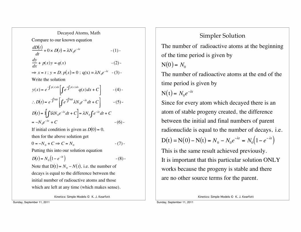
Decayed Atoms, Math

!

Compare to our known equationdD t( )dt

+ 0 " D t( ) = #N 0e$#t - (1) -

dydx

+ p(x)y = q(x) - (2) -

% x = t ; y = D; p x( ) = 0 ; q(x) = #N 0e$#t - (3) -

Write the solution

y(x) = e$ p( x )dx& e

+ p( x )dx&& q(x)dx + C' ( )

* + , - (4) -

-D t( ) = e$ 0dt& e

+ 0dt&& #N 0e$#t dt + C'

( ) * + , - (5) -

D t( ) = 1 1& #N0e$#t dt + C[ ] = #N 0 e$#t dt& + C

= $N 0e$#t + C - (6) -

If initial condition is given as D 0( ) = 0,then for the above solution get0 = $N 0 + C% C = N0 - (7) -Putting this into our solution equation

D t( ) = N0 1$ e$#t( ) - (8) -

Note that D t( ) = N0 $ N t( ), i.e. the number ofdecays is equal to the difference between theinitial number of radioactive atoms and thosewhich are left at any time (which makes sense).



Simpler SolutionThe number of radioactive atoms at the beginningof the time period is given byN 0( ) = N0

The number of radioactive atoms at the end of thetime period is given byN t( ) = N0e!"t

Since for every atom which decayed there is anatom of stable progeny created, the difference between the initial and final numbers of parentradionuclide is equal to the number of decays, i.e.

D t( ) = N 0( ) !N t( ) = N0 ! N0e!"t = N0 1! e! "t( )

This is the same result achieved previously. It is important that this particular solution ONLYworks because the progeny is stable and thereare no other source terms for the parent.



Graph of Results

!1 = 0.01, !2 = 0.05, !3 = 0.1, !4 = 0.5

N(t) = 100 [1 - exp(-!t) ]



Semi-log Graph



Scaled Graph



Example of Decayed Atoms• Problem: Sr-90 is a bone-seeking radionuclide with a half-life of 28.8 years. Assume that once strontium is deposited in bone, and that it is not excreted biologically in any appreciable way. How many decays occur as a result of the uptake of 20 microCuries of Sr-90 in 1 year? In 50 years?

• Solution:

Because of the assumption of negligible biological excretion, this is a case of simple decay. It is important to be careful with the unit conversions.

Recall that A(0) = N(0) x !

Here, ! = ln 2 / 28.8 y = 0.024/yand A = 20 x 10-3 x 3.7 x 1010 dis/s x 3600 s/h * 24 h/d x 365 d/y = 2.33 x 1016 dis/y

The total number of initial atoms is thusN(0) = A(0) / ! = (2.33 x 1016 dis/y) / (0.024/y) = 9.72 x 1017 atoms

Now, find number of decays Decayed atoms = (initial atoms) [1 - exp(-!t) ]

For one yearDecays = 9.72 x 1017 atoms [1 - exp(-0.024"1) ] decays/atom= 2.3 x 1016 decays (about 2% of the total)

For 50 yDecays = 9.72 x 1017 atoms [1 - exp(-0.024"50) ] decays/atom= 6.8 x 1017 decays (about 1/3 of the total)

In reality, the biological time course of Sr-90 in bone may be complex. It may enter blood after being trapped in the lungs from an inhalation, then be taken up in bone. It may deposit on the surface or at depth within in the bone (each with different biological excretion rates)



Decayed Atoms with Another Loss Term

• Consider the situation in which we are interested in the number of atoms which decay in the compartment of interest, but there is another loss term from the compartment

!N(t)RadionuclideN(t)

DecayedAtomsD(t)

kN(t)



Decays with Losses, Soln.

dN t( )dt

= !"N t( ) ! kN t( )# N t( ) = N0e! "+ k( )t

dD t( )dt

= +"N t( ) = "N0e! "+ k( )t

Compare to our known equationdD t( )dt

+ 0 $ D t( ) = "N0e! "+ k( )t %

dydx

+ p(x)y = q(x)

# x = t ; y = D; p x( ) = 0 ; q(x)="N0e! "+ k( )t

Write the solution

y(x) = e! p(x )dx& e+ p(x )dx&& q(x)dx + C'

()*+,

-D t( ) = e! 0dt& e+ 0dt&& "N0e

! "+ k( )tdt + C'()

*+,

D t( ) = 1 1& "N0e! "+ k( )tdt + C'

(*+ = "N0 e! "+ k( )tdt& + C

= !"

" + kN0e

! "+ k( )t + C

If initial condition is given as D 0( ) = 0, then

0 = ! "" + k

N0 + C# C ="

" + kN0

Note that "" + k

./0

123

represents the fraction of the

losses that are decay.Putting this into our solution equation

D t( ) = "N0

" + k1! e! "+ k( )t'( *+



Production with Decay

P N(t) !N(t)

P =[ ]atomstime

! " # $

% &

dN t( )dt

= P ' (N t( )

dN t( )dt

+ (N t( ) = P

x = t ; y = N; p x( ) = ( ; q(x) = P

y(x) = e' p( x)dx) e

+ p( x )dx)) q(x)dx + C* + ,

- . /

0N t( ) = e' (dt) e

+ (dt)) Pdt + C* + ,

- . /

N t( ) = e'(t P e(t) dt + C[ ] = e' (t Pe(t

(+ C

*

+ ,

-

. /

N t( ) =P(

+ Ce' (t



Production/Decay, Cont’d.


N 0( ) = N0 =P!

+ Ce"0

# C = N0 "P!


N t( ) =P!

+ N0 "P!

$ % & '

( ) e"!t

N t( ) = N0e"!t +P!

1 " e"!t( )Note that if N 0( ) = 0,

N t( ) =P!

1 " e"!t( )



Production/Decay Result

Production P = 0.02, 0.05, 0.1, and 0.5Decay ! = 0.1N(t) = P/! [1-exp(- ! t) ]



Semilog Graph



Scaled Graphs



Examples of Different Forms of Production TermsThe following are taken from Bevelacqua (2004). A key to avoiding mistakes is to continuously check for unit consistency.



Example of Production with Multiple Loss Terms

Problem: Derive an expression for N1(t) in the following model.

k2,other

k1,other

k3,other

!1

!2

!3

k1,2

k2,3

k3,4

N3(t)

N2(t)

N1(t)

kn,other Nn(t)kn-1,n

kn,n+1

!n

P1

P2

P3

Pn

***



Solution, Production with Multiple Loss TermsSolution: The compartments beyond the first compartment have no influence over it, so the problem is immensely simplified if are only concerned about the first compartment.

k1,other!1

k1,2

dN1 t( )dt

= P1 ! k1,other + " 1̀ + k1,2( )N1 t( )

This is identical to the problem just solved (productionand one loss term) except could define"effective = k1,other + " 1̀ + k1,2

The solution thus has the same form, namely

N(t) = P"

1-e-"t( )

# N1(t) = Pk1,other + " 1̀ + k1,2( )

1! exp! k1,other +"`1 + k1,2( )t$%

&'

** A generalization of this situation will be made in KJK Lecture on Long Chains



Maximum Possible Activity ProducedOne approach => Consider the activity equation with P representing the production rate expressed as atoms/time, i. e.

A(t) = ! N(t) = P x [1-exp(- ! t) ]

As t => infinity, exp(- ! t) => 0, and A(t) approaches a maximum. At the maximum

A(max) = ! N(max) = P x [1- 0 ] = P

In other words, the maximum possible activity is equal to the production rate (in atoms/time)!

Another approach is to look directly at the differential equation describing the situation, namely (on a number of atoms basis)

dN/dt = P - !N

For a maximum, slopes are zero, i.e. dN/dt = 0Thus 0 = P - !N(max) = P - A(max) #A(max) = PThis is the same result, which is reassuring.



Approaches toSteady State (Equilibrium) Problems

• Write the general temporal solution to the problem, then set the time very large to get the steady state

• Write the general differential equations, then set the differentials equal to zero. Solving will yield the answer directly! This is usually the simplest approach.



Example: Atmospheric 14C

• The production rate of 14C in the atmosphere is 1.4 x 1015 Bq/y. What is the steady state global inventory of 14C?(problem 4-39 in Cember).

Note: 14N (n, p) 14C

Here, we are given “PA”, the production rate on an activity basis. The problem is nothing more than a simple production/decay problem (just solved previously). Note that a steady state is reached for long times t, in fact we want N(t) for t=infinity. The half-life of 14C is 5700 y (from RHH), thus we have all we need to solve.

Note that the box represented here is the 14C in the atmosphere (no losses other than decay are assumed).

PA AtmosphereNatm(t)A atm(t)

!Aatm(t)



Atmospheric 14C, Solution

Let PA = !P (activity production rate) =[ ]activity

time" # $ %

& '

Using our production/decay equation (activity basis)

Aatm t( ) =PA!

1 ( e(!t( )For t ) *, 1 ( e(!t( )) 1

+ Aatm *( ) =PA! 14C

=

1.4 ,1015 Bqy

"

# $

%

& '

ln 25700 y"

# $

%

& '

=1.15 ,1019 Bq

Another approach (atom basis)dNatm t( )

dt= (!14CNatm t( ) + P = (! 14CNatm t( ) +

PA! 14C

At steady state

0 = (! 14CNatm SS( ) +PA!14C

+Aatm SS( ) =PA! 14C

=1.15 , 1019 Bq



Example of Production with Decay and Steady State

[Lamarsh Problem 3.4, p. 220]Problem: The $—-emitter 28Al (half-life 2.30 min) can be

produced by the radiative capture of neutrons by 27Al. The 0.0253 eV cross-section for this reaction is 0.23 b. Suppose that a small, 0.01-g aluminum target is placed in a beam of 0.0253 eV neutrons, % = 3 x 108 neutrons/cm2-s, which strikes the entire target. Calculate(a) the neutron density in the beam (in neutrons/cm3) (b) the rate at which 28Al is produced (in atoms/s)(c) the maximum activity (in microCuries) that can be produced in this experiment

Recall that energy and velocity are related. At thermal energies (0.0253 eV) the neutron velocity is 2200 m/s.

Other possibly useful information1 barn = 10-24 cm2

density of Al = 2.7 g/cm3

Avogadro’s number NA = 6.02 x 1023 atoms/moleNatural Aluminum is 100% Al-271 Ci = 3.7 x 1010 dis/s

Note: Burnup of the Al-27 will be neglected here.



Solution

! =ln2T1/2

=0.693

2.3min= 0.301 / min = 0.00502 / s

" thermal( ) = 0.23 b= 0.23 x 10-24 cm2

# = 3 x 108 ncm2 $ s

0.01 g AlThermal 0.0253 eV % 2200 m/s

a) Neutron density

#n

cm2 $ s&'(

)*+= neutron density x neutron velocity

= n ncm3

&'(

)*+, v cm

s&'(

)*+

-n = #v=

3 x 108 ncm2 $ s

&'(

)*+

2200 ms

&'(

)*+

100 cm1 m

&'(

)*+

= 1364 ncm3


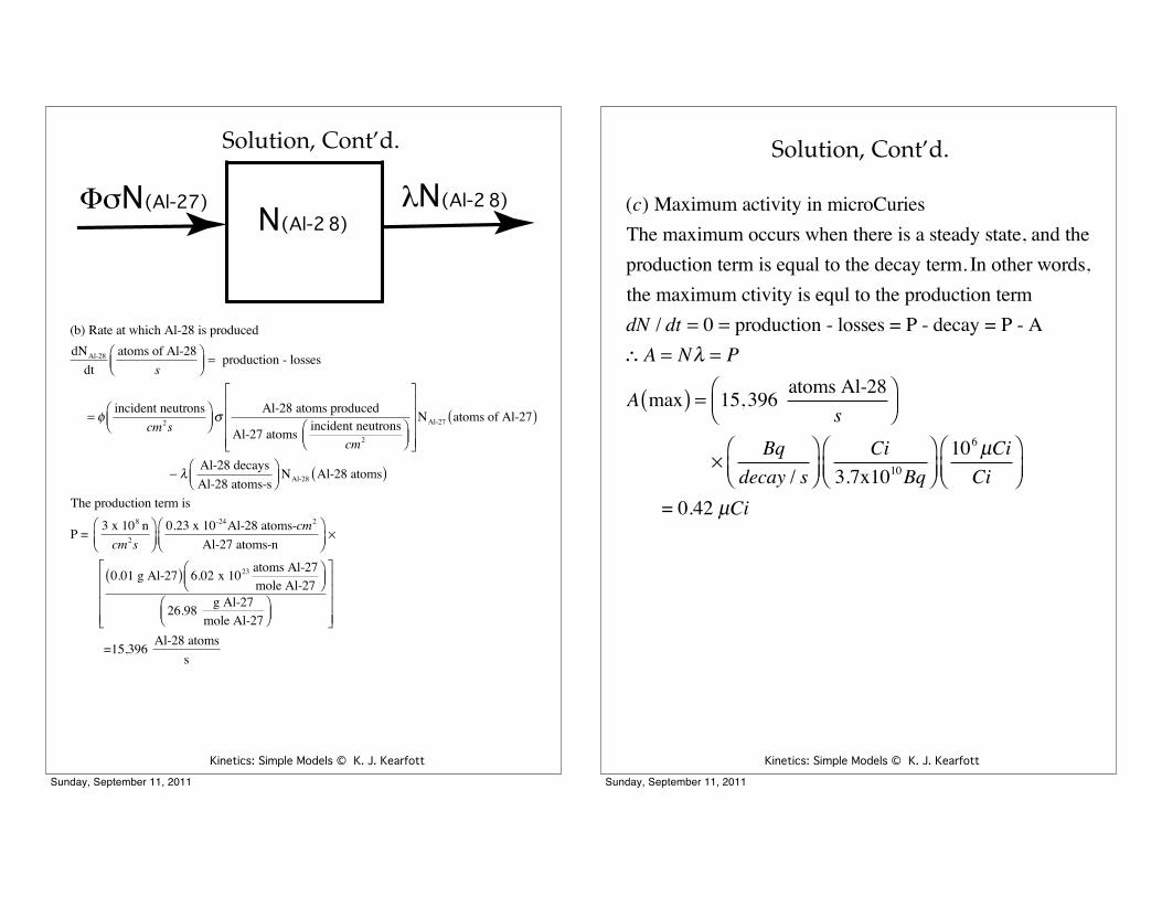
(b) Rate at which Al-28 is produced

dNAl-28

dt

atoms of Al-28

s

!"#

$%&= production - losses

= 'incident neutrons

cm2s

!"#

$%&(

Al-28 atoms produced

Al-27 atoms incident neutrons

cm2

!"#

$%&

)

*

++++

,

-

.

.

.

.

NAl-27 atoms of Al-27( )

/ 0Al-28 decays

Al-28 atoms-s

!"#

$%&

NAl-28 Al-28 atoms( )

The production term is

P = 3 x 108 n

cm2s

!"#

$%&

0.23 x 10-24Al-28 atoms-cm2

Al-27 atoms-n

!"#

$%&1

0.01 g Al-27( ) 6.02 x 1023 atoms Al-27

mole Al-27

!"#

$%&

26.98 g Al-27

mole Al-27

!"#

$%&

)

*

++++

,

-

.

.

.

.

=15,396 Al-28 atoms

s


Solution, Cont’d.

!"N(Al-27) N(Al-2 8)#N(Al-2 8)



Solution, Cont’d.

(c) Maximum activity in microCuries

The maximum occurs when there is a steady state, and the

production term is equal to the decay term. In other words,

the maximum ctivity is equl to the production term

dN / dt = 0 = production - losses = P - decay = P - A

!A = N" = P

A max( ) = 15,396 atoms Al-28

s

#$%

&'(

)Bq

decay / s

#$%

&'(

Ci

3.7x1010Bq

#$%

&'(

106µCi

Ci

#$%

&'(

= 0.42 µCi



Radiocarbon Dating• Suppose the ratio of C-14 to elemental carbon in a given type of living object, say wood, is well known and hasn’t changed over time

• Further assume that the amount of C-14 in the atmosphere is known, and easier still, has remained constant over time

• If the amount of C-14 is fixed in a living object upon its death (e.g. tree cut down and a board sawed), except for decay, then the age of the object (approximately time of death of the organism) may be determined from the following simple equation

(current ratio of C-14: C in object)

= (ratio of C-14: C in object at time of death)

* exp [ - ln (2) * (time since death) / (half-life of C-14) ]

• A good website for information about this method ishttp://www.c14dating.com/



Example of Radiocarbon DatingFor the determination of the age of an artifact using C-14 dating, the ratio of C-14 to stable carbon in the object is then compared to the ratio of C-14 to stable carbon found today. There are several assumptions, however, which must be made for C-14 dating in its simplest implementation.

Additional informationHalf-life of C-14: 5715 yearsC-14 decays 100% of the time via beta emissionProduction rate of C-14 in the atmosphere: 1.4 x 1015 Bq/yPercentage of total carbon that is C-14: 10-10 %Percentage of total carbon that is C-13: 1.07 %Percentage of total carbon that is C-12: 98.93 %Avogadro’s number: 6.02 x 1023 atoms/moleAtomic weight of carbon: 12.0107

C-14 is produced from the following reactionAtmospheric N-14 + cosmic neutron => C-14 + proton

A piece of wood found at an archeological site is analyzed. For a counting period of 20 minutes, at an efficiency of 72%, there were 423 beta counts recorded corresponding to C‑14. It is then determined that the sample contains 1.57 g of carbon. Approximately how old is the sample (expressed in years)?



Solution

! =ln2

5715 y= 1.213"10#4 / y

activity of C-14 in sample = C$yt

= 423 counts

0.72 countsemission

%&'

()*

1emissiondecay

%&'

()*

20min( )= 29.375 decays

min

atoms of C-14 in sample = A!=

29.375 decaysmin

%&'

()*

60 minh

%&'

()*

24 hd

%&'

()*

365 dy

%&'

()*

1.213"10#4 / y( ) = 1.273"1011 atoms C-14

atoms of C in sample = 1.57 g( ) 6.02 "1023 atoms

mole%

&'(

)*

12 gmole

%&'

()*

= 7.876 "1023atoms C

C-14C

%&'

()* sample today

= 1.273"1011 atoms C-14

7.876 "1023atoms C= 1.616 "10#13

C-14C

%&'

()* sample today

=C-14

C%&'

()* sample yesterday

e#!t + C-14C

%&'

()* living today

e#!t

, t =

# ln

C-14C

%&'

()* sample today

C-14C

%&'

()* living today

-

.

////

0

1

2222

!=

# ln 1.618 "10#13

10-12

%

&'(

)*

1.213"10#4 / y( )= 15,025 y + 15,000 y



Some Questions about Radiocarbon Dating

• What effect will changes in atmospheric C-14 production have on the results, and how may a correction be made for this?

• How could any losses or additions of C-14 to the object following its death be accounted for?

• For a given measurement sensitivity and error, what will be the uncertainty in the estimation of the age of the object due to the measurement uncertainties alone?

• If other radionuclides are used for this technique, then how will half-life influence accuracy and the ages which may best be determined using the method? What other factors may influence your comments?



Criticisms of RadioDating by Anti-Evolutionists

• See evolution-facts.org or Ferrell (2001)

Problems with all dating methods1. Each system has to be a closed system. Nothing can

contaminate any of the parents or the daughter products while they are going through their decay process. No piece of rock cannot for millions of years be sealed off from other rocks, water, chemicals, and changing radiations from outer space

2. Each system must initially have contained none of its daughter products. This can in no way be confirmed.

3. The process rate must always have been the same. The decay rate must never have changed. All radioactive clocks, including C-14, have always had a constant decay rate unaffected by external influences. This is not true because decay rate may be changes if a) material is bombarded by high energy particles from space; b) there is a nearby radioactive material emitting radiation, c) as a result of physical pressure, d) as a result of contact with chemicals

4. Changes in the blanket of atmosphere surrounding the planet would affect results by changing the amount of cosmic radiation

5. Any change in the Van Allen belt would change the amount of cosmic radiation

6. Things started at the beginning, no daughter products were present, only elements at the top of the radioactive decay chain were present



Criticisms Specific to C-14 DatingThe following assumptions1. Atmospheric carbon is constant2. Oceanic carbon is constant3. Cosmic radiation is constant4. Rate of formation and decay of C-14 is constant5. The decay rate of C-14 has never changed6. Nothing has ever contaminated any specimen

containing C-147. No seepage of water or other factor has brought

additional C-14 to the sample since death8. The fraction of C-14, which the living thing possessed

at death, is known today9. The half-life of C-14 is accurate10. Nitrogen is the precursor to C-14, thus nitrogen in

the atmosphere must have been constant11. Instrumentation is precise, working properly, and

analytic methods are always carefully done12. Technique always yields the same results on the same

sample or related samples that are obviously part of the same larger sample

13. The earth’s magnetic field was the same in the past as it is today



Production Term with Gas Mixing in a Room

• Suppose a radioactive gas is leaking from a container into a room of volume V at some rate L (atoms/time). Suppose that the turnover rate of air in the the room is R (fraction of volume/time). Write an equation for the activity concentration in the room as a function of time. (Assume instantaneous and complete mixing of room air).

The compartment represents radioactive atoms in the air of the room. Losses are both by decay and by removal with air leaving the room. Entrance is through leakage from thecontainer.

L(atoms/time) !NRoom Air

N(atoms)A(activity)V(volume)

RN



Gas Mixing, Soln.

Problem on a "number of atoms" basisdN t( )dt

= L ! RN t( ) ! "N t( )

= L ! (R+ ")N t( )For N(0) = 0

# N t( ) = LR + "

1 ! e!(R+ ") t[ ]On an activity concentration basisA t( )V

="N t( )V

="L

V R + "( )1 ! e!(R+ ") t[ ]

Note that this expression is the same as thatobtained for production with decay, butsubstitute (R + " ) = "effective everywhere for "and use L for the production term (previously P).



Simple Activation

• Suppose a radionuclide is produced by bombarding a target which produces a radionuclide. This is also a simple case of production/decay (if we neglect the burnup of the target).

The compartment is the amount of product actually present at any time

!"Ntarget ProductNproduct

#Nproduct



Simple Activation, Soln.activation problemsRate of interactions = flux ! cross section

"particlescm2 sec

# $ % &

' ( ! )

cm 2 ! interactionsbombarding particles! target nuclei#

$ %

&

' (

= ")interactions

sec ! target nuclei#

$ %

&

' (

The cross section is a probability of interaction perbombarding particle flux per target nucleus. It is a property that has been measured and is tabulated

in the RHH and the "Barn Book" (1 b = 10-24 cm2 ).Production rate of product is thus

P = ")interactions

sec ! target nuclei#

$ %

&

' ( !Ntarget target nuclei( )

= ")Ntargetinteractions

sec# $ % &

' (

If N target is constant, then our previous equation

for simple production/decay applies, and we have

Nproduct t( ) =P

*product

1 + e+* p roductt( )

Nproduct t( ) =")N target

*product

1 + e+* product t( )The maximum product for simple activation occursfor t ,-, or t large w.r.t. the product half - life, and is equal to

Nproduct tmaximum = t-( ) =")Ntarget

*product



Activation with Burnup• Suppose that there were a finite number of target atoms for an activation, and we wanted to account for the effects of losses of these atoms during the activation process. Our model is now a two-compartment model.

!"Ntarget ProductNproduct

#Nproduct

TargetNtarget



SolutionProduction rate of product varies as f(t), i.e.

P = !"Ntarget t( )interactions

sec# $ % &

' (

We therefore have, for the target compartmentdN target t( )

dt= )P = )!"N target t( )

This is the same form as simple decay, withthe solutionNtarget t( ) = Ntarget 0( )e)!"t

Our equation for the product compartment isdNproduct t( )

dt= P ) *Nproduct t( ) = !"Ntarget t( ) ) *Nproduct t( )

Substituting in our equation for Ntarget t( )

dNproduct t( )dt

= !"Ntarget 0( )e) !"t ) *Nproduct t( )

Now, put in form we know the solution todNproduct t( )

dt+ *Nproduct t( ) = !"Ntarget 0( )e)!" t

Compare to Bernoulli' s equationx = t ; y = Nproduct; p x( ) = * ; q(x) = !"Ntarget 0( )e)!" t

Write down the solution

y(x) = e) p( x)dx+ e

+ p( x )dx++ q(x)dx + C, - .

/ 0 1

2Nproduct t( ) = e) *dt+ e

+ *dt++ !"Ntarget 0( )e)!"tdt + C, - .

/ 0 1



Solution, Cont’d.Simplifying yields

Nproduct t( ) = e! "t #$N target 0( ) e"t e!#$ t% dt + C[ ]= e!"t #$Ntarget 0( )

e " ! #$( )t

" !#$+ C

&

' (

)

* +

Nproduct t( ) = #$Ntarget 0( )e!#$t

" ! #$+ Ce! "t

If initial condition is given as Nproduct 0( ) = 0,

then for the above solution get

Nproduct 0( ) = 0 =#$Ntarget 0( )" ! #$

+ C

, C = !#$Ntarget 0( )" ! #$


Nproduct t( ) = #$Ntarget 0( )e!#$t

" ! #$!#$Ntarget 0( )" !#$

e!"t

Nproduct t( ) =#$N target 0( )" !#$( )

e!#$t ! e!"t( )

where " = "product

Recall that neglecting burnup (i.e. for the conditions forwhich " >> #$ and -#$t- 0) we got the following

Nproduct t( ) =#$Ntarget

"product

1 ! e!" product t( )



Activation with Burnup Results

Accounting for target burnup, have

Nproduct t( ) =!"Ntarget 0( )#product $!"( )

e$!"t $ e$# product t( )Neglecting target burnup, have

Nproduct t( ) =!"Ntarget

#product

1 $ e$# product t( )

Important note: For activation with target burnup, the “saturation” or maximum activity is not reached. Furthermore, in the case that the number of target atoms is small, this effect is even more pronounced.



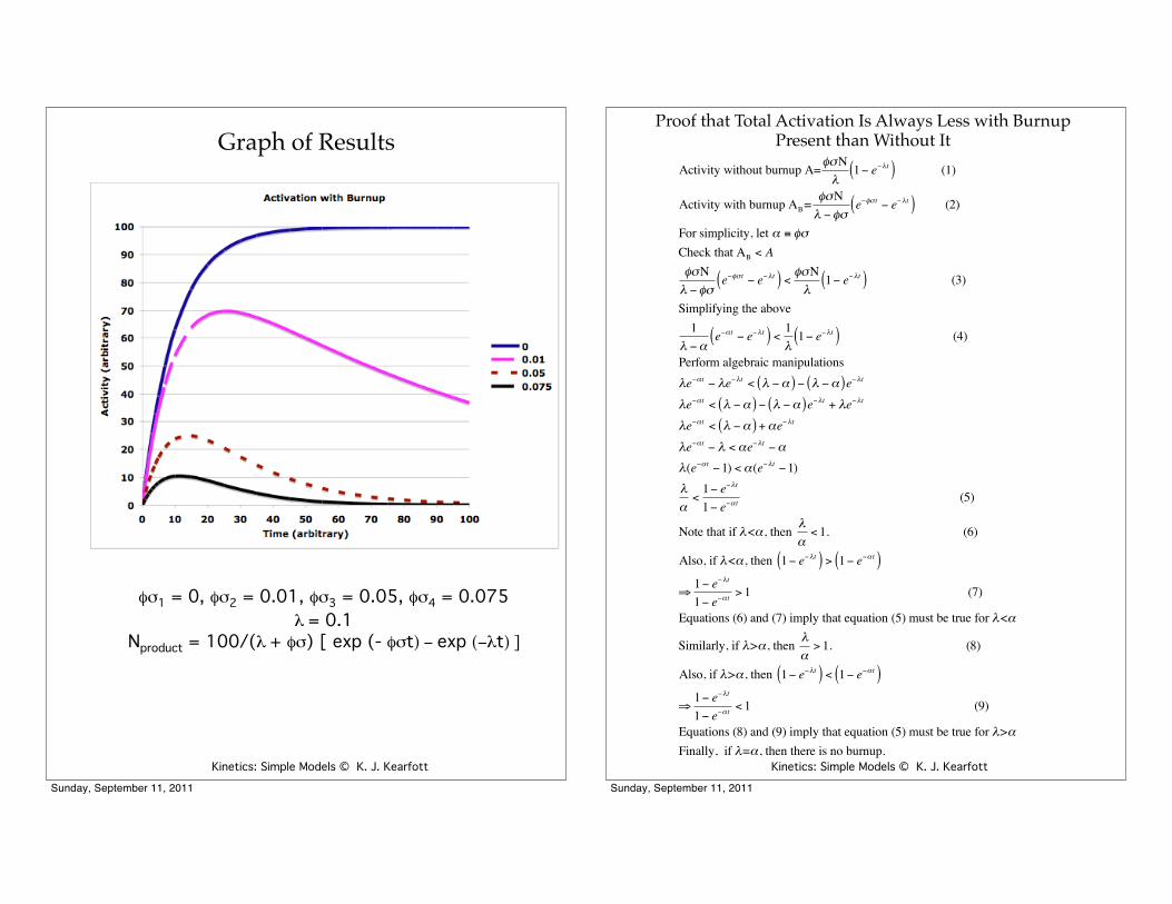
Graph of Results

%&1 = 0, %&2 = 0.01, %&3 = 0.05, %&4 = 0.075! = 0.1

Nproduct = 100/(! + %&) [ exp (- %&t) ' exp ('!t) ]



Proof that Total Activation Is Always Less with Burnup Present than Without It

Activity without burnup A=!"N#

1$ e$#t( ) (1)

Activity with burnup AB= !"N# $!"

e$!" t $ e$#t( ) (2)

For simplicity, let % & !"

Check that AB < A!"N# $!"

e$!" t $ e$#t( ) < !"N#

1$ e$#t( ) (3)

Simplifying the above1

# $%e$% t $ e$#t( ) < 1

#1$ e$#t( ) (4)

Perform algebraic manipulations#e$% t $ #e$#t < # $%( ) $ # $%( )e$#t

#e$% t < # $%( ) $ # $%( )e$#t + #e$#t

#e$% t < # $%( ) +%e$#t

#e$% t $ # <%e$#t $%#(e$% t $1) <%(e$#t $1)#%<

1$ e$#t

1$ e$% t (5)

Note that if #<%, then #%< 1. (6)

Also, if #<%, then 1$ e$#t( ) > 1$ e$% t( )

'1$ e$#t

1$ e$% t> 1 (7)

Equations (6) and (7) imply that equation (5) must be true for #<%

Similarly, if #>%, then #%> 1. (8)

Also, if #>%, then 1$ e$#t( ) < 1$ e$% t( )

'1$ e$#t

1$ e$% t< 1 (9)

Equations (8) and (9) imply that equation (5) must be true for #>%Finally, if #=%, then there is no burnup.



Maximum for Activation with Burnup

Nproduct t( ) =!"Ntarget 0( )# product $ !"( )

e$!"t $ e$# productt( )Differentiate w.r.t. time, and set equal tozero to find the time of maximum productdNproduct t( )

dt= 0

=!"N target 0( )# product $!"( )

$!"e$!"t max + # producte$ #product tmax( )

%!"e$!"tmax = #product e$# producttmax

!"# product

= e !" $#product( )tmax

ln!"#product

&

' (

)

* + = !" $ #product( )tmax

, tmax =

ln !"#product

&

' (

)

* +

!" $ #product( )The maximum is thus equal to

Nproduct tmax( ) =!"Ntarget 0( )# product $ !"( )

e$!"tmax $ e$# producttmax( )



Note on Steady State,Equilibrium, and Saturation

• If times are long with respect to the decay constant, and either complete decay or buildup occurs, then there is a substantial simplification of formulae

==> At steady state, equilibrium, and saturation,the [ 1 - exp ( - ! t ) ] terms approach one

• Under such circumstances have the following

Activity produced (and present) P / !

Total number of decays A / !



Hints on Solving Kinetics Problems

• Be sure that the units match up whenever any equation is used

• Be careful with equations; they may be stated either on an activity or on an atom basis

• Often an equation may be written simply based upon an understanding of the overall form expected for the solution

(e.g. exponential, 1-e-kt, what the maximum should be, etc.)

• Always verify that the conditions for which the equation was derived apply to the situation at hand



Summary of Kinetics Formulae: Decay

Simple decay

N t( ) = N0e!"t

Decay with another loss term

N t( ) = N0e! " + k( )t

Decayed atoms

D t( ) = N0 1 ! e! "t( )Total possible number of decaysD #( )= N0

Decayed atoms with another loss term

D t( ) = "N0

" + k1 ! e! " + k( )t[ ]

Total possible number of decays when loss term

D t( ) = "N0

" + k



Summary of KineticsFormulae: Production

Production without decayN t( ) = PtProduction with decay

N t( ) = P!

1 " e"!t( )Production with decay, with initial activity

N t( ) = N0e"!t +P!

1 " e"!t( )Steady state for production and decay

N SS( ) =P!

Production with additional loss terms

N t( ) = P! + k( )

1" e" ! + k( ) t[ ]Sunday, September 11, 2011


Summary of Kinetics Formulae: Activation

Activation, neglecting target burnup

Nproduct t( ) =!"Ntarget

#product1 $ e$# productt( )

Steady state (or maximum) activation product

Nproduct SS( ) =!"Ntarget

# product

Activation, with target burnup

Nproduct t( ) =!"Ntarget 0( )# product $ !"( )

e$!"t $ e$# productt( )



Things to Know• Radiocarbon dating assumes that C-14: C ratio is constant in living objects, that C-14 in the atmosphere has been constant over time, and that objects no longer exchange carbon with the environment (and there are not C-14 production terms) once the object is no longer living



Definitions to Know

activationBernoulli’s equationboundary conditionsbuildupcompartmentcross sectiondecaydecay chaindecay constantdependent variabledeterminantdual decayeigenvalueequilibriumfirst order linear differential equationfission productsfluxhalf-lifeindependent variableinitial conditions



Definitions, Cont’d.

matrix solution of system of equationsnonlinear equationsparent radionuclidepartial decay constantprogeny radionuclideradiocarbon datingradiation intensityrate transfer constantssaturationspecific activitysteady statetarget burnup



Exercises

• Write the set of differential equations corresponding to any first order linear model

• Solve simple sets of equations involving differential equations of simple form

• Recognize simple decay and decay with production problems and be able to solve quickly



Suggested ABHP Part II Problems

1975: 6a+b, 161976: 2a, 8a1978: 1d 1979: 1a+b+c, 7(know what MPC is) 1981: 1a+b, 7a, 12a+c1982: 10a1983: 13a+b1984: 2a+b1986: 1a+b1987: 5a+b, 8a+b1988: 9f+g+h1989: 5a+b, 7a+c+e, 10b+c+d+e+f, 11b+c+d1990: 1a+b, 3d, 4a+b, 8f+g, 91991: 11a+b+d1992: 1, 9a+b, 10a, 12a1993: 8a+b+c, 12a+b1994: 7a+d



References• Bevelacqua, J. J. “Production equations in health physics”, Radiation Protection Management, vol. 20, no. 6, pp. 9-14, 2004.

• Cember, H. Introduction to Health Physics,Third Edition, McGraw-Hill, New York, NY, 1996.

• Ferrell, V., The Evolution Cruncher, Evolution Facts, Inc., Altamont, TN, 2001

• Friedman, M. H., Principles and Models of Biological Transport, Springer-Verlag, New York, NY, 1986.

• Godfrey K., Compartmental Models and Their Application, Academic Press, New York, NY, 1983.

• Iyengar, S. S., Computer Modeling of ComplexBiological Systems, Chemical Rubber Company Press, Boca Raton FL, 1984.

• Kajiya, F., Kodama, S., Abe, H., CompartmentalAnalysis: Medical Applications and TheoreticalBackground, Karger, New York, NY, 1984

• Krane, K. S. Introductory Nuclear Physics, John Wiley and Sons, New York NY, 1988.



References, Cont’d.• J. R. Lamarsh, A. J. Baratta, Introduction to Nuclear Engineering, 3rd Edition, Prentice Hall, Upper Saddle River, NJ, 2001.

• H. J. Moe, Operational Health Physics Training, Argonne National Laboratory, ANL-88-26, U.S. Department of Energy, National TechnicalInformation Service, Springfield, VA 22161.

• Shipley, R. A., Clark, R. E., Tracer Methods forin Vivo Kinetics: Theory and Applications,Academic Press, New York NY, 1972.

• Skrable, K., French, C., Chabot, G., Major, A.,A general equation for the kinetics of linearfirst order phenomena and suggested applications,Health Physics 27: 155-157, 1974.

• Stella II, software from High PerformanceSystems, 45 Lyme Road, Hanover NH 03755,telephone (603) 643-9636, fax (603) 643-9502,AppleLink: X0858

• Radiological Health Handbook (RHH 1970), U.S. Dept. of Health, Education, and Welfare, 1970.



References, Cont’d.

• B. Shleien, L. A. Slaback, B. K. Birky (RHH 1998), Handbook of Health Physics and Radiological Health, Third Editions, Williams and Wilkins, Baltimore, MD, 1998.

• Tuli, J. K., Nuclear Wallet Card, National NuclearData Center, Brookhaven National Lab, Upton, NY, 1990.

• J. E. Turner, Atoms, Radiation, and Radiation Protection, Pergamon Press, New York, NY, 1986.


kinetics simple models

Documents