1

Kinetic-Ion Simulations Addressing Whether Ion Trapping Inflates Stimulated

Brillouin Backscattering Reflectivities

B.I. Cohen and E. A. Williams

University of California Lawrence Livermore National Laboratory

P.O. Box 808, Livermore, CA 94551

and H. X. Vu

University of California, San Diego, La Jolla, CA 92093

Abstract

An investigation of the possible inflation of stimulated Brillouin backscattering

(SBS) due to ion kinetic effects is presented using electromagnetic particle simulations

and integrations of three-wave coupled-mode equations with linear and nonlinear models

of the nonlinear ion physics. Electrostatic simulations of linear ion Landau damping in

an ion acoustic wave, nonlinear reduction of damping due to ion trapping, and nonlinear

frequency shifts due to ion trapping establish a baseline for modeling the electromagnetic

SBS simulations. Systematic scans of the laser intensity have been undertaken with both

one-dimensional particle simulations and coupled-mode-equations integrations, and two

values of the electron-to-ion temperature ratio (to vary the linear ion Landau damping)

are considered. Three of the four intensity scans have evidence of SBS inflation as

determined by observing more reflectivity in the particle simulations than in the

corresponding three-wave mode-coupling integrations with a linear ion-wave model, and

the particle simulations show evidence of ion trapping.

2

I. INTRODUCTION

The nonlinear interaction of intense, coherent electromagnetic waves in high

temperature plasmas plays an important role in laser fusion.1,2 Stimulated backscattering

of the incident electromagnetic wave by electron plasma waves, stimulated Raman

backscattering (SRS), and by ion acoustic waves, stimulated Brillouin backscattering

(SBS), are of particular interest because the backscattering can damage the final optics of

the laser and degrade the symmetric illumination (direct or indirect) of the laser-fusion

target.3,4 Stimulated backscattering instabilities in laser plasmas have been the object of

more than thirty years of intense research in experiments, analytical theory, and

simulations. The new work presented here addresses specific aspects of the saturation of

stimulated Brillouin backscattering in which nonlinear kinetic ion physics is important.

Our previous research on SBS has examined the role of nonlinear ion physics in

the saturation of SBS in one and two spatial dimensions, and with the inclusion of ion-ion

collisions and spatial inhomogeneity.5,6,7,8,9 Vu and co-workers have elucidated the

effects of wave breaking and ion trapping in SBS with particle simulations.10 Recent

work by Vu, Dubois, and Bezzerides has demonstrated with particle simulations and

detailed modeling that SRS can exhibit reflectivities significantly in excess of those

derived from models in which the electron plasma wave is assumed to be small amplitude

and nonlinearities are absent.11 The research by Vu and co-workers on SRS was

motivated by experimental observations of SRS reflectivities much in excess of linear

theory reported by Montgomery and co-workers.12 The simulations and modeling in Ref.

11 make the case that electron trapping, which nonlinearly reduces electron Landau

damping13 and produces a nonlinear frequency shift14,15,16 in the electron plasma wave,

3

can produce kinetic inflation of SRS because the linear SRS gain depends inversely on

the damping of the electron plasma wave when the electron plasma wave is strongly

damped. The effects of ion trapping on ion acoustic waves are quite analogous to electron

trapping effects on electron plasma waves, 17,5 Evidence of ion trapping has been

observed frequently in simulations4-10 of SBS and in experiments.18 We are thus

motivated to examine whether ion trapping in the SBS ion acoustic waves can

nonlinearly reduce ion wave damping and inflate the SBS reflectivities.

Here we present an investigation of SBS using electromagnetic particle

simulations including nonlinear ion kinetic effects and integrations of three-wave

coupled-mode equations with a reduced model of the nonlinear ion physics addressing

whether kinetic inflation of SBS can occur. To establish a baseline for modeling the

electromagnetic SBS simulations, we have undertaken electrostatic simulations to

directly measure the linear ion Landau damping of small-amplitude ion acoustic waves

and the nonlinear reduction of damping and emergence of a nonlinear frequency shift due

ion trapping in large-amplitude ion waves. Systematic scans of the laser intensity have

been undertaken with both one-dimensional electromagnetic particle simulations and a

coupled-mode-equations model to study SBS; and two values of the electron-to-ion

temperature ratio (to vary the linear ion Landau damping) are considered. Three of the

four intensity scans yield significant evidence of SBS inflation as determined by

observing more reflectivity in the particle simulations (which show evidence of ion

trapping) than in the corresponding three-wave mode-coupling integrations with a linear

(small-amplitude) ion-wave model. Integrations of the three-wave mode-coupling

equations with a simplified nonlinear model incorporating ion-trapping effects are useful

4

in elucidating the effects of nonlinearities on SBS. Our studies also demonstrate the

importance of kinetic simulations of SBS in giving guidance to reduced models.

The paper is organized as follows. Section I introduces the subject matter and its

motivation. Section II comments on how collisions can affect ion-trapping effects and

describes the particle simulation and three-wave-coupling models. Section III presents

one-dimensional electrostatic simulations of small and large-amplitude ion waves to

establish the linear damping of the small-amplitude waves and the nonlinear damping and

frequency shifts of large-amplitude waves. In Sec. IV we report the results of four scans

of laser intensity in electromagnetic particle simulations of SBS and the corresponding

three-wave mode-coupling modeling. Conclusions are presented in Sec. V.

II. PARTICLE SIMULATION AND THREE-WAVE MODE COUPLING MODEL

A. Particle-in-cell simulations with ion-ion collisions

Particle-in-cell simulations with kinetic ions and Boltzmann electrons described

elsewhere5,11 are used here to study stimulated Brillouin backscattering (SBS) with

nonlinear kinetic ion effects. The electrons are modeled as a fluid with a Boltzmann

response to the longitudinal electric fields. The fluid electrons respond to the

perpendicularly polarized pump and scattered electromagnetic waves, provide the

transverse current in Maxwell’s equations, and produce the ponderomotive potential that

perturbs the electron density and drives the SBS ion waves. There is no collisional

absorption of the electromagnetic waves in this model. We impose an explicit Fokker-

Planck ion-ion collision operator9 in some of the simulations. An important consequence

of ion-ion collisions is that they provide a detrapping mechanism for resonant ions that

5

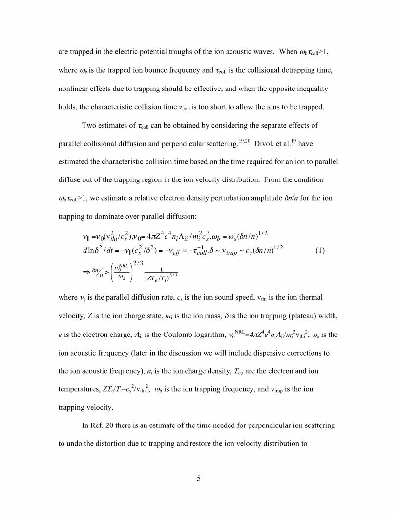
are trapped in the electric potential troughs of the ion acoustic waves. When ωbτcoll>1,

where ωb is the trapped ion bounce frequency and τcoll is the collisional detrapping time,

nonlinear effects due to trapping should be effective; and when the opposite inequality

holds, the characteristic collision time τcoll is too short to allow the ions to be trapped.

Two estimates of τcoll can be obtained by considering the separate effects of

parallel collisional diffusion and perpendicular scattering.19,20 Divol, et al.19 have

estimated the characteristic collision time based on the time required for an ion to parallel

diffuse out of the trapping region in the ion velocity distribution. From the condition

ωbτcoll>1, we estimate a relative electron density perturbation amplitude δn/n for the ion

trapping to dominate over parallel diffusion:

!

" || =" 0(vthi2/cs2)," 0= 4#Z

4e4ni$ii /mi

2cs3,%b =%s(&n /n)

1/2

d ln&2 /dt = '" ||(cs2/&2) = '"eff ( ')coll

'1,& ~ vtrap ~ cs(&n /n)

1/2

*&nn

>" 0NRL

%s

+

, -

.

/ 0

2 /31

(ZTe /Ti )5 / 3

(1)

where ν|| is the parallel diffusion rate, cs is the ion sound speed, vthi is the ion thermal

velocity, Z is the ion charge state, mi is the ion mass, δ is the ion trapping (plateau) width,

e is the electron charge, Λii is the Coulomb logarithm, ν0NRL=4πZ4e4niΛii/mi

2vthi2, ωs is the

ion acoustic frequency (later in the discussion we will include dispersive corrections to

the ion acoustic frequency), ni is the ion charge density, Te,i are the electron and ion

temperatures, ZTe/Ti=cs2/vthi

2, ωb is the ion trapping frequency, and vtrap is the ion

trapping velocity.

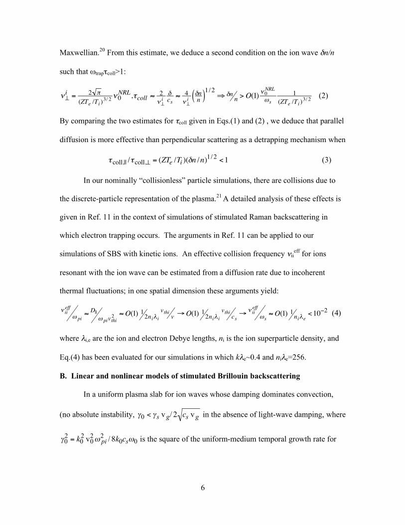
In Ref. 20 there is an estimate of the time needed for perpendicular ion scattering

to undo the distortion due to trapping and restore the ion velocity distribution to

6

Maxwellian.20 From this estimate, we deduce a second condition on the ion wave δn/n

such that ωtrapτcoll>1:

!

"#i = 2 $

(ZTe /Ti )3/ 2

"0NRL

,%coll &2

"#i

'cs& 4

"#i

'nn( )1/2

('nn

>O(1)" 0NRL

)s

1

(ZTe /Ti )3/ 2

(2)

By comparing the two estimates for τcoll given in Eqs.(1) and (2) , we deduce that parallel

diffusion is more effective than perpendicular scattering as a detrapping mechanism when

!

"coll,|| /"coll,# = (ZTe /Ti )($n /n)1/2

<1 (3)

In our nominally “collisionless” particle simulations, there are collisions due to

the discrete-particle representation of the plasma.21 A detailed analysis of these effects is

given in Ref. 11 in the context of simulations of stimulated Raman backscattering in

which electron trapping occurs. The arguments in Ref. 11 can be applied to our

simulations of SBS with kinetic ions. An effective collision frequency νiieff for ions

resonant with the ion wave can be estimated from a diffusion rate due to incoherent

thermal fluctuations; in one spatial dimension these arguments yield:

!

" iieff

# pi$D||# pivthi

2 $O(1) 12ni%i

vthiv&O(1) 1

2ni% i

vthics&

" iieff

#s$O(1) 1

ni%e<10

'2 (4)

where λi,e are the ion and electron Debye lengths, ni is the ion superparticle density, and

Eq.(4) has been evaluated for our simulations in which kλe~0.4 and niλe=256.

B. Linear and nonlinear models of stimulated Brillouin backscattering

In a uniform plasma slab for ion waves whose damping dominates convection,

(no absolute instability,

!

"0 < "s v g/ 2 cs v g in the absence of light-wave damping, where

!

"02

= k02

v02# pi

2/ 8k0cs#0 is the square of the uniform-medium temporal growth rate for

7

SBS1-3), the intensity gain exponent for convective amplification of the SBS

backscattered electromagnetic wave is given by1-3

!

!

GSBSI

= 18

v02

ve2

nenc

"s# s

"0Lx

vg (1+k2$e2)

(5)

The gain exponent is an important parameter in characterizing the conditions for SBS.

Here γs is the ion wave damping rate, Lx is the length of the plasma, ω0 is the laser

frequency, v0 is the electron quiver velocity in the laser field, ve is the electron thermal

velocity, vg is the group velocity of the backscattered wave, ωpi is the ion plasma

frequency, k0 is the wavenumber of the laser, and ne/nc is the ratio of the electron density

to the critical density (where the laser frequency equals the electron plasma frequency).

If the ion wave in SBS remains relatively small in amplitude and is heavily

damped (

!

"0 < "s v g/ 2 cs v g ), then Eq.(5) describes the exponential amplification of the

backscattered wave for weak backscatter, i.e., power reflectivities R<<1. The backscatter

amplification comes at the expense of pump depletion, which must be taken into

consideration for finite R. An analytical solution for pump depletion in one spatial

dimension and in the limit

!

"0 < "s v g/ 2 cs v g has been given by Tang22 describing the

reflectivity if a steady state is reached:

R(1-R)+R0R=R0exp[(1-R)G] (6)

where G for SBS is the gain given by Eq.(5) and R0 is the ratio of the intensity of the

backscattered wave to the incident laser intensity at the boundary opposite the incident

plane. For R<<1, R~R0exp(G). Equation (6) is a transcendental equation for R given R0

and G, which is most easily solved for G as a function of R given R0. We shall compare

the Tang formula, Eq.(6), to the time-averaged reflectivities of the saturated SBS in our

8

simulations. We note that the only nonlinearity in the Tang formula is pump depletion,

and the ion wave is taken to be linear.

If ion trapping is significant, a number of new effects emerge that change the

character of the ion wave. The ion wave Landau damping is expected to be reduced as

the trapping distorts the velocity distribution, and there is also a nonlinear frequency

shift,5-9,13-17,19 Δωnl/ωs =−η|δn/n|1/2 , where η is a dimensionless coefficient that in the

simplest limit is given by7,14-17 η=

!

"O(1)v#3$2 f /$v2where f is the unperturbed velocity

distribution function. While the reduction in the damping might be expected to increase

the SBS gain, the frequency shift may produce a gain reduction due to detuning, i.e.,

intuitively, one might expect G∝1/γs ⇒1/(γs2+ Δωnl

2)1/2. If there is little or no detuning

effect, and if there is no new ion damping mechanism engendered by other nonlinearities,

then there is a basis for expecting an increase in the effective SBS gain due to the effects

of trapping through the reduction in ion wave Landau damping. In this situation an

inflation of the SBS reflectivity might be observed as in the case of SRS reported

experimentally12 and in recent simulation work.11 Understanding the linear and nonlinear

ion wave dissipation is a key element in assessing whether inflation of SBS is occurring.

Particle simulations of SBS typically see bursty reflectivities and no steady state.

The ion-wave model in the particle simulations naturally retains convection, whose

neglect as in the Tang model would be especially suspect if trapping is causing a

reduction of the ion wave damping. Thus, we are motivated to model SBS with a set of

one-dimensional coupled-mode equations retaining time dependence and convection, and

with some nonlinear modifications in the ion-wave density perturbation equation to

9

capture the effects of ion trapping. The coupled-mode equations derive straightforwardly

from well-established theory:1,3,4,23,24

!

""t

+ vg0""x( )a0 = #ic0($ne /ne)a1

""t# vg1

""x( )a1% = ic1($ne /ne)a0

%

c0 =& pe2/&1,c1 =& pe

2/&0,&0 =&1 +&s,vg 0,1 = k0,1c

2/&0,1 ' vg ,a0,1 = E0,1

(7)

for the pump and backscattered electromagnetic waves, where ωpe is the electron plasma

frequency; E0,1 are the slowly varying, complex-valued amplitudes for the transverse

electric fields, δne is the slowly varying, complex-valued amplitude of the electron

density perturbation; and vg is the group velocity of the light waves; and equations for

linear ion waves:

!

""t

+ cs""x

+ #s( )$ne / ne = %ic2a0a1& + Snoise

c2 = v02'0's

4 ve

2E00

2 '1

,#s = #LD + ( ii,Snoise = noise

(8)

and nonlinear ion waves:

!

""t

+ cs""x# i$%nl + &nl( )'ne / ne = #ic2a0a1

( + Snoise

&nl = &LD exp(# dt%b

2))0

t* + + ii,%b =%s 'ˆ n e / ne

1/ 2

,'ˆ n e = ('ne #'nnoise,0)

>

$%nl = #,%b[1# exp(# dt%b

2)0t* )]

(9)

where γnl is the nonlinear ion wave damping rate, γs is the linear ion wave damping, ωb is

the ion trapping frequency, νii is the ion wave damping due to collisions, Snoise represents

the thermal noise source present in the particle simulations,10,21Δωnl is the nonlinear

frequency shift, and Δωnl=0 is an option in the nonlinear ion model to emphasize

“inflation” effects. Based on the calculations in Refs. 13-16, the Landau damping

10

nonlinearly relaxes over a few trapped ion bounce periods and the nonlinear frequency

shift is established on the same time scale. The noise source is given by the simple

model: Snoise=Anoiseexp(iΘ) withΘ=2πr(t), where r(t)∈[0,1] is randomly chosen at every

time step.

We integrate these equations with an explicit, finite-difference, predictor-

corrector scheme using Δx=vg Δt. The incident pump and backscattered waves in Eq.(7)

are advected from left to right and right to left, respectively, along the characteristics of

the equations with the right sides evaluated explicitly using a predictor-corrector iteration

to approximately center the evaluation. The sound wave convection term is generally a

small term for

!

"0 < "s v g/ 2 cs v g and is treated explicitly with central differencing in

space. The high-frequency coupled-mode equations admit an action conservation law:

!

""t (J0 + J1) + (vg 0

""x J0 # vg1

""x J1) = 0 (10)

where the wave-action densities for the pump and backscattered waves are defined as

!

J0,1 " a0,1

2/(2#$0,1) . With 100 spatial cells, the relative action conservation error was

less than 1% in all cases. As a check of the coupled-mode equations, we considered a

test case using the linear ion-wave model, a pump-wave intensity below the threshold for

absolute instability, ne/ncrit=0.1, a Be plasma, ZTe/Ti=6.24, Te=2 keV, νii/ωs=0,

Lx/λ0~300, very weakly seeded backscatter so that pump depletion is negligible, no IAW

noise source (Snoise=0), Δx/Lx=0.01, γLD/ωs=0.097, and v0/ve=0.2033 For this test case, we

expect the coupled-mode equations to settle into a steady state with convective growth of

the backscatter and a spatial growth rate1 for the amplitude a1 given by

κconv=γ2SBS/(γLDvg1)=5.04×104m-1, where γSBS is the homogeneous-medium convective

11

temporal growth rate and GISBBS=2κconvLx from Eq.(5). This is in good agreement with

the coupled-mode-equations integration which yielded a spatial growth rate of

5.0×104m-1 after a steady state was reached (~35 ps).

III. Linear and Nonlinear Ion Wave Features in PIC Simulations

The coupled-mode equations introduced in the preceding section are used to

model the more complete particle simulations of SBS. For the results of the coupled-

mode equations to agree reasonably well with the kinetic simulations, it is important to

use accurate values for the linear and nonlinear ion wave damping and the frequency

shifts. To this end we calibrate the ion-wave model in the coupled-mode equations with

two types of electrostatic ion wave simulations: initial-value of simulations of undriven,

small-amplitude, ion acoustic waves to determine the linear ion wave damping directly

(which can be compared to linear theory) and ponderomotively driven ion waves at finite

amplitude to motivate our model of nonlinear SBS ion waves.

A. Ion wave linear damping

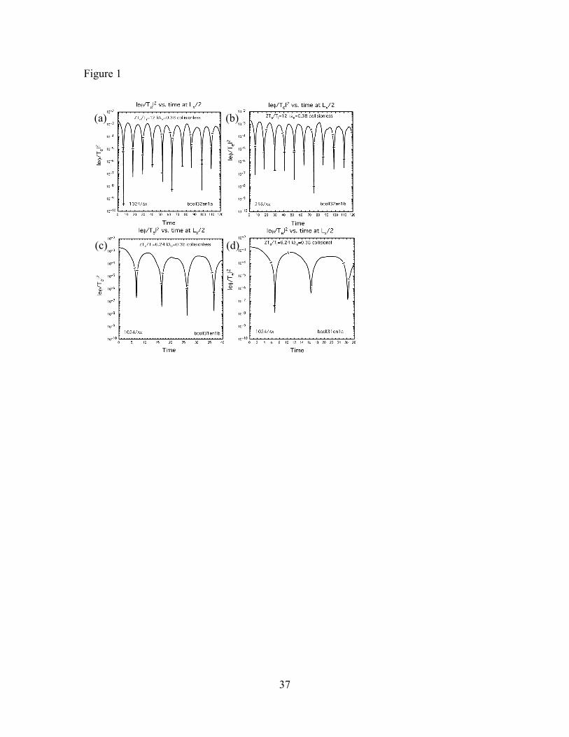
By initializing a small-amplitude, sinusoidal displacement of the ions in a particle

simulation to launch a standing wave, a direct measurement of the ion wave frequency

and damping rate can be made, which is then compared to linear theory. Figure 1 shows

the results from one-dimensional BZOHAR simulations of small-amplitude, ion acoustic,

standing waves with ne/ncrit=0.1, a Be plasma, ZTe/Ti=12 and 6.24, Te=2 keV, νii/ωs=0,

Lx/λIAW~40, kΔx=0.04, kλe=0.38, and 256 and 1024 particles per cell. For ZTe/Ti=12, the

BZOHAR simulations agree relatively well with linear theory (including ion thermal

effects): ωs=0.269, γs=0.0041 as compared to ωs=0.28, γs=0.0044 for 1024/Δx particles

12

and ωs=0.272, γs=0.005 for 256/Δx particles. Note that in BZOHAR’s units, the ion

plasma frequency

!

" pi = Z / A = 2 / 3 for a Be plasma (Z=4, A=9). For ZTe/Ti=6.24,

BZOHAR simulation again agrees relatively well with linear collisionless theory:

ωs=0.293, γs=0.0284 as compared to ωs=0.31, γs=0.0287 for 1024/Δx particles

(collisionless) and ωs=0.31, γs=0.029 for 1024/Δx particles (with collisions,

ν0NRL/ωs=0.02). The RPIC10 particle simulation for the ZTe/Ti=6.24 case yielded γs/ωs

=0.097 for 256/Δx particles using quadratic interpolation for the ion charge density

calculation (BZOHAR uses linear interpolation and γs/ωs =0.092 was observed). With

fewer particles per cell, the effective collisional diffusion due to discrete particle effects

is larger;11,21 and we expect that the simulations will yield higher damping rates. Ion-ion

collisions tend to increase the ion wave damping rates, but there are some subtleties.25

These test cases provide values for the linear damping rates of the ion acoustic waves

needed for the modeling of the SBS simulations in Sec. IV.

B. BZOHAR simulations of driven ion waves: nonlinear frequency shift and

damping with no imposed ion collisions

We next consider BZOHAR simulations of ponderomotively driven ion waves.

We undertook two simulations with values of ZTe/Ti=12 and 6.24. Both simulations

exhibit evidence of ion trapping, e.g., an ion velocity tail is produced and there is

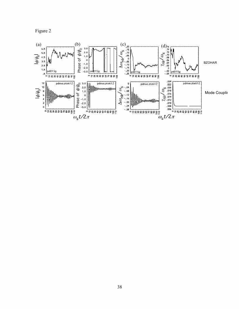
flattening of the velocity distribution for v~cs . In Figure 2 we show the results of a one-

dimensional simulation with ne/ncrit=0.1, a Be plasma, ZTe/Ti=12, Te=2 keV, driver turn-

on time ωs0τdron=2.5, νii/ωs=0, Lx/λs~5, kΔx=0.25, kλe=0.4, driver potential eφ0/Te=0.02

and frequency Ω=ωs0=kcs/(1+ k2λe2)1/2 As a diagnostic we use a Taylor-series expansion

13

of the longitudinal dielectric response with respect to εnl(ωnl,κ)=0 and solve for

ωnl= Reωl+Δωnl+iγnl in terms of other quantities using the derived relation:26,5

!

ke2"e

2#($,%+ i& /&t) ˜ ' (%,$;t) ( ke2"e

2 &#nl&)

(%*)nl + i& /&t) ˜ ' (%,$;t) = * ˜ ' 0(%,$;t) (11)

From the amplitude and phase of the electric potential φ relative to φ0, we use Eq.(11) to

identify approximate values for the nonlinear frequency shift Δωnl and damping rate γnl.

After relaxation of the transients, ωs0t/2π > 50, |eφ/Te|~0.1±0.01, the phase of the electric

potential relative to the driving potential approaches π, γnl/ωs0 ⇒ O(0±0.02) and Δωnl/ωs0

⇒ -0.12±0.01 (and both are not steady). This can be compared to linear theory,

γl/ωs0=0.015, and nonlinear trapping theory,13-16 Δωnl/ωs0=-η|eφ/Te|1/2~-0.12 for η=0.4

and γnl⇒0. The full value of the nonlinear frequency shift is realized in the simulation.

The damping generally decreases in magnitude in the simulation as time progresses and

becomes oscillatory, but the dissipation is positive on average over the simulation.

In Figure 3 we show the results of a one-dimensional BZOHAR simulation with

ne/ncrit=0.1, a Be plasma, ZTe/Ti=6.24, Te=2 keV, driver turn-on time ωs0τdron=2.5,

νiiNRL/ωs0=0, Lx/λs~5, kΔx=0.25, kλe=0.4, driver potential eφ0/Te=0.02 and frequency

Ω=ωs0=kcs/(1+ k2λe2)1/2 Again using Eq.(11), we deduce values for Δωnl and γnl For

ωs0t/2π > 45, |eφ/Te|⇒0.09, the phase of the response approaches π, γnl/ωs0 ⇒

O(0.01±0.02) and Δωnl/ωs0 ⇒ -0.15 The frequency shift and damping rates are not

steady, and can be compared to linear theory, γl/ωs0=0.097, and nonlinear trapping

theory,13-16 Δωnl/ωs0=-η|eφ/Te|1/2~-0.27 for η=0.9 and γnl⇒0. However, the ion wave

dissipation remains positive on average. ~60% of the frequency shift expected from

nonlinear trapping theory is observed in the simulation.

14

In Figs. 2 and 3 we also show the results of integrating Eq.(9) from the coupled-

mode equations with a fixed ponderomotive driving potential (with a finite turn-on time,

ωs0τdron~2) suppressing the dynamics of the electromagnetic waves. In the integration of

Eq.(9) we used η=0.4 and η=0.54 and γnl/ωs0=0.015 (relaxes to zero) + 0.008 (residual)

and γnl/ωs0=0.08 (relaxes to zero) + 0.02 (residual) for ZTe/Ti=12 and 6.24, respectively,

as motivated by the BZOHAR simulation results and the frequency-shift and nonlinear-

damping diagnostic. The integration of the coupled-mode equations in this case yields

qualitatively similar results compared to the BZOHAR results after initial transients

relax. Late in time there is some semi-quantitative agreement of the ion-wave

magnitudes and the nonlinear frequency shifts. To the extent that the damping rates late

in time are small compared to magnitude of the frequency shift and positive, the phases in

the kinetic simulation are ≤π. It is typical that the damping and frequency shift

diagnostic based on Eq.(11) yields effective damping rates that are much larger than one

would expect based on linear theory early in time, which then decrease to smaller values

as transients relax and the velocity distributions flatten due to trapping. Meanwhile the

frequency shifts in the BZOHAR simulations deduced from the diagnostic qualitatively

resemble those built into the nonlinear ion wave model in the coupled-mode equations.

The relative magnitudes of |φ/φ0| and phases in the particle simulations and the couple-

mode-equation integrations are similar after the initial transients.

The results of the two simulations for steadily driven ion waves indicate that there

is a general relaxation of the ion-wave dissipation and that a nonlinear frequency shift

results that approaches the value suggested by trapping theory. However, neither the

damping nor the frequency shift is steady; and the time-averaged damping is positive.

15

The reduced model based on Eq.(9) with a defined ponderomotive driving potential

captures some of the important phenomenology at least qualitatively.

IV. PIC Simulations of SBS and Three-Wave Coupled-Mode Integrations

In this section we present particle simulations of SBS in one spatial dimension

and accompanying integrations of the coupled-mode equations that model the particle

simulations. In each of the four studies the incident laser intensity is scanned

corresponding to an interesting range of linear gains. As the laser intensity is increased,

the SBS reflectivities increase; and nonlinearities become evident.

The rationale for the four test cases is as follows. Firstly, if inflation of SBS

occurs in a specific plasma condition, is that occurrence exceptional? To address this

question in a limited parameter study, four series of intensity scans were examined. Two

values ZTe/Ti=6.24 and 12 are considered, corresponding to relatively strong and weak

ion Landau damping. For ZTe/Ti=6.24, we consider one case in which there are imposed

ion-ion collisions (Case 1) and another case in which there are no imposed collisions

(Case 2). The collisions increase the ion wave damping, which reduces the SBS gain

exponent and is expected to reduce the reflectivities. For ZTe/Ti=6.24, we also

investigate a case with no imposed ion collisions in which the discrete particle noise and

the concomitant fluctuation-driven diffusion have been reduced significantly (Case 3). In

Case 3, we expect that trapping can occur at lower ion wave amplitudes because the

collisional detrapping is weaker, which circumstance might allow inflation to onset at

lower laser intensities. However, the SBS exponentiates from the significantly lower

thermal fluctuations for the density perturbations, which leads to a lower saturated

16

reflectivity for the same value of the gain parameter as in Case 2. For ZTe/Ti=12 and no

imposed collisions (Case 4), the ion wave linear damping is significantly reduced, which

means that the linear gains for SBS are significantly higher for the same values of the

laser intensity. The simulations address whether the reduced ion Landau damping in

Case 4 makes it easier for inflation to occur.

A. Case 1: ZTe/Ti=6.24 with ion-ion collisions using BZOHAR

All of the SBS simulations share the following parameters: the laser wavelength

corresponds to λ0=0.35 µm, ne/ncrit=0.1, a Be plasma, Te=2 keV, Lx/λ0~300, and

k0Δx=k0λe=0.2. For this first case ZTe/Ti=6.24, and the ion-ion collision frequency

νiiNRL/ωs0=0.28, where

!

"iiNRL

=4#Zi

4e4ni$ ii

mi2vi3, the total relative linear ion wave

damping is γstot/ωs=0.112,25 from the trapping theory Δωnl/ωs0=-0.9(δn/n)1/2, and the

simulation durations correspond to τsim~60ps. The length of the simulation is chosen to

approximate a single speckle length, Lx~8f2λ0, where f =f/#~6 is the f-number. The ion-

ion collisions were imposed using the Fokker-Planck collision model outlined in Ref. 9.

For δn/n > 0.015, which in this series of simulations occurs for (v0/ve)2>0.02, the ion

response should be in a trapping-dominated physics regime based on Eqs.(1) and (2).

The intensity scan v0/ve=0.0707 - 0.2828 corresponds to linear gains 1 – 16. Note that

v0/ve≈6(I0λ02/1014Wµm2/cm2)1/2/Te(eV)1/2. Data from the BZOHAR simulations and

coupled-mode-equations integrations are shown in Fig. 4. The time-averaged BZOHAR

reflectivities follow the Tang formula (RTang) using the linear gains relatively well with a

value of R0 so that the resulting reflectivities match the time-averaged BZOHAR

reflectivities at the lowest intensities. However, the reflectivities are not steady in the

simulations, which motivates the mode-coupling, time-dependent analysis. If the

17

saturated reflectivities were relatively steady and compared well with the Tang formula

using the linear ion wave damping rate, then this would be a basis for concluding that

there was no significant inflation of SBS.

The BZOHAR simulation peak and time-averaged reflectivities are compared

with coupled-mode equation predictions using the linear and nonlinear IAW models in

Figs. 4-7. The amplitude Anoise of the noise source in Eqs.( 8) and (9) is set by fitting the

resulting peak reflectivities to match the BZOHAR peak reflectivities at the lowest

intensities for which the SBS signal is above the noise (backscattering off the thermal

noise in the density fluctuations). As the value of v0/ve increases in Fig. 4a, we see that

the BZOHAR peak and time-averaged reflectivities significantly exceed the reflectivities

produced by the coupled-mode equations with the linear ion-wave model, which gives

evidence of inflation. Use of the nonlinear ion-wave model in the coupled-mode

equations yields higher reflectivities and a better match to the BZOHAR data. The

“inflation” model (Δωnl=0) reflectivities are much too high.

In Fig. 5 the peak relative electron density perturbations at x=Lx/4 in the

BZOHAR simulations are compared to couple-mode-equation results as a function of the

pump-wave intensity for linear, nonlinear, and “inflation” IAW models. A spatially local

comparison is made difficult because the coupled-mode-equation IAW amplitudes are

strongly spatially dependent and peak sharply at the left side of the plasma where the

pump enters when SBS is strong. Furthermore, the local spatial variability in the

unfiltered density perturbation amplitudes is 25-50% throughout. We note that while the

coupled-mode equations with the nonlinear model lead to reflectivities that better match

18

the BZOHAR data, use of the linear ion-wave model better matches the ion-wave

amplitudes in this particular case.

Figures 6 and 7 show results from a BZOHAR simulation with v0/ve=0.1414,

ZTe/Ti=6.24, νiiNRL/ωs0=0.28, τsim~40ps and the corresponding coupled-mode-equation

integrations with linear and nonlinear ion-wave models. Distortion of the ion velocity

distribution due to trapping is evident in Fig. 6f. Evidence of coupling of the SBS ion

wave to subharmonic features emerges in the electrostatic streak spectrum in Fig. 6e,

which may be a manifestation of a secondary instability, e.g., two-ion-wave decay.5

Mode coupling and two-ion-wave decay processes are omitted from the SBS coupled-

mode equations. These processes are a source of nonlinear dissipation for the SBS ion

wave, which can reduce the SBS.5 The mode-coupling results in Fig. 7 capture the bursty

time dependence of the BZOHAR reflectivity and the ion wave amplitude in a general

sense. We note that the first large burst of SBS reflectivity in Fig. 6a in BZOHAR has

the highest reflectivity as is frequently observed in other one and two-dimensional

BZOHAR SBS simulations.6,9 This is not the case in the results from the coupled-mode

equations whose bursts of reflectivity do not decrease in magnitude and sometimes

increase in time (Fig.7a,c). We have documented that the decrease in the magnitude of

the reflectivity bursts in time in the BZOHAR simulations correlates with the occurrence

of the coupling/decay of the principal SBS ion wave to lower-frequency, longer-

wavelength ion waves.5.7 We believe that the absence of the coupling of ion waves to

other ion waves, including two-ion-wave decay, likely accounts for why the reflectivity

bursts are not observed to decrease in magnitude after the first burst in the mode coupling

calculations presented here.

19

B. Case 2: ZTe/Ti=6.24 with no ion collisions using BZOHAR

In Fig. 8 we show the results of BZOHAR simulations and corresponding mode-

coupling-equation integrations scanning laser intensity with ZTe/Ti=6.24, Te=2 keV, no

imposed ion collisions, γLD/ωs0=0.092, Δωnl/ωs0=-0.9(δn/n)1/2 , τsim~60ps. The BZOHAR

simulations show ion trapping (Fig. 9), and reflectivities higher than the mode coupling

model yield with linear ion waves. In this test case and the two that follow with no

imposed ion-ion collisions, evaluation of Eqs.(1) and (2) suggests that the ion wave

amplitude thresholds set in for |δn/n| values <1% in order to be in the ion-trapping-

dominated limit. The intensity scan v0/ve=0.0707 - 0.2828 corresponds to linear gains 1 –

12. The peak reflectivities and many of the time-averaged reflectivities exceed the Tang

formula using the linear gain (Fig. 8a). The peak reflectivities follow the predictions of

the coupled-mode equations with the nonlinear ion-wave model (Fig. 8b). Use of the

nonlinear and inflation (Δωnl/ωs=0) ion-wave models in the coupled-mode equations

give higher reflectivities than the reflectivities produced with the linear ion-wave model.

The reflectivities using the inflation model are significantly higher than the BZOHAR

values (Fig. 8c). Because the BZOHAR peak reflectivities exceed the coupled-mode-

equation reflectivities using the linear IAW model, this suggests that there is some

inflation of SBS in this intensity scan. In addition, many of the BZOHAR time-averaged

reflectivities observed exceed the Tang formula using the linear ion wave damping rate.

Figure 8d shows the mode-coupling reflectivities as functions of laser intensity

using a nonlinear ion-wave model amended to include some residual damping (Δωnlr≠0,

“nlr-c” data), Imω/ωs0=0.082 (relaxes to zero due to trapping)+.01 (residual, does not

relax). We note that the collisional discrete particle effects, Eq.(4), motivate the

20

assumption of the residual damping and its approximate magnitude. Furthermore, there

is again some evidence of mode coupling and two-ion-wave decay in the BZOHAR

electrostatic streak spectrum shown in Fig. 9. The choice of the magnitude of the

residual ion wave damping in the mode-coupling model could be made on the basis of a

careful assessment of the ion wave damping based on theoretical arguments, or

measurements or inferences of the ion wave damping in the kinetic simulations, or by

fitting the mode-coupling results (by varying the residual damping) to the results of the

kinetic simulations, or some other logic. We did a little exploration of the sensitivity of

the mode-coupling results to varying the residual damping, but this exploration was not a

systematic optimization with respect to the value of the residual damping. The value of

the residual ion wave damping used here should be considered as illustrative and

reasonable given Eq.(4).

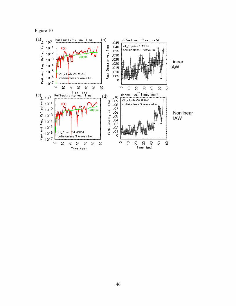
In Fig. 10 are shown plots of the reflectivities and density perturbations at x=Lx/4

as functions of time from coupled-mode integrations with linear and nonlinear (nlr-c) ion-

wave models. The reflectivities in the mode-coupling integrations and in BZOHAR are

similarly bursty, and the density perturbation amplitudes increase in amplitude with

respect to time in both examples in Fig. 10. However, the BZOHAR reflectivity bursts

tend to decrease in amplitude with respect to time while the mode-coupling reflectivities

increase. We present the peak density perturbation amplitudes at x=Lx/4 as functions of

(v0/ve)2 for BZOHAR and the mode-coupling models in Fig. 11. We note that the mode-

coupling data using the nonlinear ion wave model with residual damping (nlr-c) is in

better agreement with both the BZOHAR reflectivities (for (v0/ve)2 > 0.015) and density

perturbations than the data from the other ion-wave models (Figs. 8d and 10). The

21

overall results indicate that the mode-coupling equations augmented with a nonlinear

model of the ion waves capture important features in the BZOHAR simulations but do

not reproduce everything.

C. Case 3: ZTe/Ti=6.24 with no ion collisions (RPIC simulation)

We also undertook a series of simulations with the same parameters as in Case 2

using the RPIC particle simulation code,10,11 which uses quadratic interpolation to

compute the ion density and has a lower thermal fluctuation level than does BZOHAR

which uses linear interpolation.11,21 In the RPIC, one-dimensional simulations, the

parameters again were ZTe/Ti=6.24, with no imposed ion-ion collisions, τsim~120-300ps,

γLD/ωs=0.097 (measured independently), and Ncell=256. The laser intensities were

scanned over v0/ve=0.037 - 0.26 (6×1013W/cm2 - 3×1015W/cm2) corresponding to linear

gains 1 - 12. With a lower-amplitude thermal noise source, smaller reflectivities and

saturated ion wave amplitudes result than were observed in the BZOHAR simulations.

In Fig. 12 we observe that the time-averaged reflectivities follow the Tang

formula using the linear gain, but the reflectivities are non-steady. There are a few peak

reflectivities in Fig. 12a above the predictions of the mode-coupling model using a linear

IAW model (which may suggest that there is some inflation), but the mode-coupling

time-averaged reflectivities with a linear ion-wave model agree well with most of the

RPIC simulation results. The mode-coupling equations using the nonlinear ion-wave

models slightly over-estimate the particle simulation peak and time-averaged reflectivies

in Figs. 12b and 12c.

If we include some residual dissipation for the ion waves in the nonlinear ion-

wave model (model nlr-c), then the mode-coupling peak and time-averaged reflectivities

22

reproduce the particle simulation reflectivities relatively well using γtot/ωs=0.082 (relaxes

to 0) + 0.015 (residual damping) and retaining a finite nonlinear frequency shift. In fact,

both the nlr-c and linear ion wave mode-coupling models fit the particle simulation

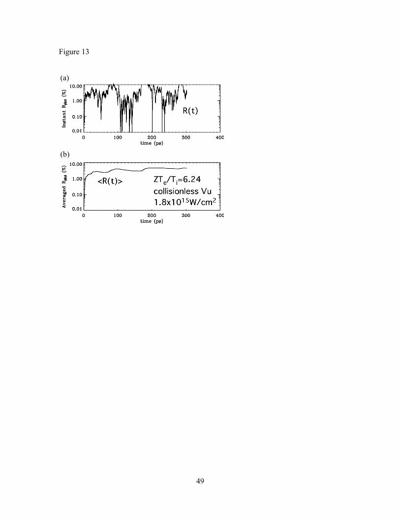
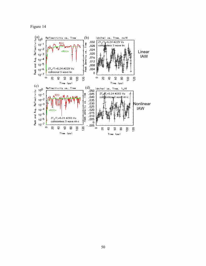
reflectivities quite well. In Fig. 13 we show an example of the reflectivities as functions

of time from a specific particle simulation and in Fig. 14 the corresponding mode-

coupling calculations for I0=1.8×1015 W/cm2. The mode-coupling calculations in Fig. 14

are similarly bursty, and the magnitudes of the reflectivities are in relatively good

agreement. The magnitudes of the reflectivity bursts in the RPIC kinetic simulation and

in the mode- coupling integrations here are significantly smaller than those in Case 2 and

do not increase in time. The amplitudes of the density perturbations observed in the

mode-coupling-equations integrations are similarly smaller here as compared to those in

Case 2 for the same laser intensity (and, hence, smaller linear gain exponent) correlating

with the reduced thermal noise source in the RPIC simulations out of which the SBS

grows. With smaller ion-wave amplitudes, the nonlinear ion-wave effects are weaker.

We conclude that in this RPIC series of particle simulations and the corresponding mode-

coupling integrations there is almost no evidence of inflation, and the mode-coupling-

equations integrations (linear and nlr-c) capture the bursts of reflectivity relatively well.

The power spectrum of the density fluctuation, |δne(k,ω)|2, for a representative

simulation (I0=1.9×1015 W/cm2) is shown in Fig. 15 in two ranges of k and ω for clarity.

The top panel shows a non-stimulated noise spectrum, corresponding to the usual linear

dispersion of IAWs for kλDe<0.2, and a stimulated IAW spectral streak at kλDe~0.38

corresponding to the SBS-generated IAW and its subsequent ion trapping-induced

frequency shift. This spectral streak feature is analogous to the Langmuir wave streaks

23

observed in previous RPIC simulations of backward SRS in the (electron) trapping

regime.27 The lower panel of Fig. 15 shows the same power spectrum, but in a smaller

range of k and ω. One interesting feature can be seen in this contour plot: the spectral

streak is actually composed of several distinct "islands." Each of these "islands" can be

correlated to a distinct SBS spatiotemporal pulse moving across the simulation domain.

For each RPIC simulation performed, the density fluctuation at a fixed location

(for the cases reported here, this location is 25µm away from the laser entrance boundary)

as a funtion of time is recorded. Three significant quantities are calculated from this set of

data: the maximum density fluctuation (δnmax), the average of the temporal density

maxima (δnmean), and the root-mean-square (rms) of the temporal density maxima (δnrms).

From the temporal density fluctuation at a fixed location δne(xfixed,t), a set of local

maxima of |δne(xfixed,t)| is computed. The largest among these local maxima is then

computed and is called, for the lack of better terms, the maximum density fluctuation

δnmax. δnmean and δnrms are computed as the unweighted arithmetic mean and the rms,

respectively, of the set of local maxima. δnmax, δnmean, and δnrms are quantitative measures

of the strength of the SBS-generated IAWs. A summary of the results for our RPIC

simulations is shown in Fig. 16, along with analagous quantities from three-wave

coupled-mode simulations. Similar to the comparison of the BZOHAR ion wave

amplitudes to those from the coupled-mode-equations integrations, there is qualitative

agreement between the RPIC ion wave amplitudes and those from the coupled-mode-

equations modeling. We note that the nonlinear mode-coupling model with residual

dissipation (nlr-c) matches both the reflectivities and the trends of the ion wave

amplitudes vs. laser intensity relatively well (Figs. 12d and 15). Although there is no

24

indication of inflation in the SBS reflectivities in this RPIC series, the results of the

coupled-mode-equation integrations using the nlr-c ion wave model and the significant

ion wave amplitudes and evidence of ion trapping effects in the RPIC simulations suggest

that ion-wave kinetic nonlinearities are significant elements in these simulations and the

plasma response is not linear.

D. Case 4: ZTe/Ti=12 with no ion collisions using bZOHAR

In this last series of BZOHAR simulations we consider a case with much weaker

ion Landau damping and no imposed collisions. The parameters are ZTe/Ti=12, no

imposed collisions, γsLD/ωs0=0.015, Δωnl/ωs0=-0.3(δn/n)1/2, and τsim~35-80ps. We scan

laser intensities such that v0/ve=0.04 - 0.1, which corresponds to linear gains ~2 – 15.

The time-averaged BZOHAR reflectivities mostly follow the Tang formula using the

linear gains in Fig. 17, but the reflectivities are non-steady. The peak and time-averaged

reflectivities substantially exceed the coupled-mode-equations peak reflectivities using

the linear ion-wave model (Fig. 17a), and there is evidence of ion trapping (Fig. 18),

suggesting that nonlinearities are inflating the SBS reflectivities.

Integrating the coupled-mode equations with Δωnl=0 (“inflation”) and damping

that relaxes to zero leads to reflectivities that are systematically too high compared to

BZOHAR data (Fig. 17b). The nonlinear IAW models (nlr and nlr-c) that retain

nonlinear frequency shifts fit bZohar reflectivity data better than the “linear” and

“inflated” models. The nlr-c model includes a small effective collisional damping rate

that models discrete particle effects (νii/ωs=0.008). Use of the nlr-c model leads to a

better fit to the bZohar reflectivities and the δn/n data in Fig. 18, while the coupled-

mode-equation results with the linear IAW model do not fit as well.

25

Results from a BZOHAR simulation with v0/ve=0.06, ZTe/Ti=12, ν0NRL/ωs=0, and

τsim~100ps are shown in Fig. 19. Evidence of mode coupling and two-ion-wave decay

again emerges in the electrostatic streak spectrum late in time. The distortion of the

velocity distribution due to trapping is clearly evident. The corresponding mode-

coupling SBS calculations with the same parameters are shown in Fig. 20 with the linear

ion-wave model and with the nonlinear ion-wave model (nlr-c) having finite residual

damping νii/ωs=0.008 The nonlinear ion model leads to higher IAW amplitudes and

reflectivities than with the linear IAW model. The nonlinear ion-wave model with

residual damping (nlr-c) compares more favorably with BZOHAR data for both the

reflectivities and the ion wave density perturbations in Figs. 17-20.

V. Conclusions

Four series of particle simulations and accompanying coupled-mode-equation

integrations were undertaken in which the laser intensity was scanned looking for

evidence of SBS inflation due to nonlinear effects. For the cases with ZTe/Ti=6.24 with

and without imposed collisions using BZOHAR (Cases 1 and 2), we saw significant

evidence of inflation and generally similar behavior, although Case 2 had larger linear

gains and slightly higher saturated reflectivities. The ion-wave peak amplitudes in Case 1

are smaller than in the collisionless case, Case 2. In Case 3 (ZTe/Ti=6.24 with no

imposed collisions, using the RPIC simulation code), the significantly lower thermal

fluctuations due to discrete-particle noise led to a factor of 10 lower thermal Thomson

backscattering noise signal in the reflectivities than in Case 2, and approximately a factor

of 10 lower reflectivities overall. With ZTe/Ti=12 in Case 4 using BZOHAR with no

26

imposed collisions, the results are qualitatively similar to Case 2 with ZTe/Ti=6.24, in the

magnitude of the inflation effects, the significant reflectivities and the ion trapping effects

observed, the evidence of mode coupling and/or two-ion-wave decay, and the general

importance of nonlinearities.

Over the range of parameters examined in three of the four intensity scans using

our particle simulations of SBS there is evidence of inflation, i.e., either the peak or both

the peak and time-averaged reflectivities in the particle simulations exceed the

reflectivities resulting from the corresponding coupled-mode-equation integrations with a

linear IAW model for some range of pump-wave intensities. The amount of inflation in

the reflectivities varies from a factor of a few to a factor of ten. In the Case 3 intensity

scan the SBS grows from a smaller thermal fluctuation level leading to lower

reflectivities and lower saturated ion-wave amplitudes with weaker nonlinear effects and

little or no evidence of inflation.

It is interesting that the predictions of the Tang formula using the linear ion wave

damping rate compare relatively well with the time-averaged reflectivities in the particle

simulations. Because the reflectivities are quite time dependent in these simulations, the

Tang formula is not really applicable. Furthermore, the Tang formula ignores all

nonlinearities in the ion waves and in the ion velocity distribution perturbations, although

it does capture the important pump-depletion nonlinearity. Perhaps the success of the

Tang formula in predicting the time-averaged reflectivities observed in the particle

simulations is only fortuitous.

The coupled-mode-equation integrations with linear and nonlinear models for the

ion waves have been used to compare to the particle simulation results. The nonlinear

27

ion-wave models embody the basic phenomenology of ion trapping which can

nonlinearly reduce the ion Landau damping and produce nonlinear frequency shifts.

Because the value of the ion wave damping is a very influential parameter in the

modeling, we have undertaken direct particle simulations of ion waves to measure the ion

wave damping in the small-amplitude, linear-physics regime. We have also performed

simulations of ponderomotively driven ion waves in electrostatic simulations to assess

finite-amplitude effects on the ion wave damping and to measure frequency shifts

directly. Our modeling of the particle simulations with the coupled-mode equations

indicates that use of a linear ion-wave model is inadequate for most of the simulation

results when both the reflectivities and the ion-wave density perturbations exceed a few

per cent. In three of the four intensity scans (Test Cases 1, 2, and 4), use of the nonlinear

ion-wave models (“nlr” in Case 1 and “nlr-c” in Cases 2 and 4) in the mode coupling

equations leads to results that better match the particle simulation results. In Test Case 3,

there is little difference in the results of the coupled-mode equations using the linear and

“nlr-c” models, both of which lead to reflectivities that match both the peak and time-

averaged reflectivities well. However, use of the “nlr-c” model agrees better with the

observed ion wave amplitudes than does using the linear ion wave model in Case 3. The

agreement of the coupled-mode equations with the particle simulation reflectivities in

Cases 2 and 4 also was improved with additions of small amounts of residual dissipation

or effective collisionality (“nlr-c” model, which takes into account the discrete-particle

effects in the PIC simulations or other sources of residual IAW damping). In all of the

cases studied, use of a nonlinear ion-wave model that completely suppresses the

28

nonlinear frequency shift leads to overestimates of the reflectivities and the ion wave

amplitudes.

The experience here with the reduced modeling of SBS using coupled-mode

equations augmented with a nonlinear model of the ion waves is sufficiently encouraging

to motivate further work with the coupled-mode equations in which we extend and

improve the coupled-mode-equations model as guided by kinetic particle simulations.

The extensions address certain physics omissions. We have begun incorporating a model

of ion-wave mode coupling and/or two-ion-wave decay in the SBS coupled-mode-

equations model, because we believe that ion wave mode coupling/two-ion-wave decay is

a potentially important ion wave dissipation mechanism. Another omission in our mode-

coupling model is that the ion trapping flattens and distorts the ion velocity distribution

function, which distortions survive when the ion wave relaxes unless there are ion side

losses or collisional relaxation. The distortion of the ion velocity distribution alters the

damping rate of the ion wave and its frequency.7,19 A reduced model of the ion trapping

effects on SBS that includes the evolution of the flattening of the ion velocity distribution

by introducing equations for the growth and relaxation of the ion velocity plateau width

has been introduced in Ref. 19. We will compare the results of the coupled-mode-

equations model to kinetic SBS simulations incorporating these extensions in the future.

The one-dimensional particle simulations of SBS and the modeling with coupled-

mode equations presented here suggest that inflation can occur. Our previous work in

two-dimensional SBS simulations6,9 has indicated that ion trapping effects are just as

vigorous and the effects of ion wave mode coupling and two-ion-wave decay are

profound in saturating SBS in two spatial dimensions. Whether the inflation observed

29

here in one dimension survives in two dimensions remains to be investigated. We note

that we are unaware of any experimental evidence for significant kinetic inflation of SBS.

Acknowledgements

This work was performed under the auspices of the U.S. Dept. of Energy by the

University of California Lawrence Livermore National Laboratory under contract No. W-

7405-ENG-48. H. X. Vu was supported by the NNSA under the Stewardship Science

Academic Alliances Program through DOE Research Grant # DE-FG52-

04NA00141/A000. We thank Don Dubois, Laurent Divol, Bruce Langdon for their

interest and encouragement, Bedros Afeyan for suggesting comparing coupled-mode

equation integrations to the particle simulation results, and Dick Berger for useful input,

suggestions, and a careful reading of the manuscript.

References

1W. L. Kruer, The Physics of Laser Plasma Interactions (Addison-Wesley, Reading, MA,

1988).

2J. D. Lindl, P. Amendt, R. L. Berger, S. G. Glendinning, S. H. Glenzer, S. W. Haan, R.

L. Kauffman, O. L. Landen, and L. J. Suter, Phys. Plasmas 11, 339 (2004).

3J. Drake, P. Kaw, Y. C. Lee, G. Schmidt, C. S. Liu, and M. N. Rosenbluth, Phys. Fluids

17, 778 (1974)

4D. W. Forslund, J. M. Kindel, and E. L. Lindman, Phys. Fluids 18, 1002 (1975); and

ibid. 18, 1017 (1975).

5B. I. Cohen, B. F. Lasinski, A. B. Langdon, and E. A. Williams, Phys. Plasmas 4, 956

(1997).

30

6B. I. Cohen, L. Divol, A. B. Langdon, and E. A. Williams, Phys. Plasmas 12, 052703

(2005).

7E. A. Willams, B. I. Cohen, L. Divol, M. R. Dorr, J. A. Hittinger, D. E. Hinkel, A. B.

Langdon, R. K. Kirkwood, D. H. Froula, and S. H. Glenzer, Phys. Plasmas 11, 231

(2004).

8L. Divol, B. I. Cohen, E. A. Williams, A. B. Langdon, and B. F. Lasinski, Phys. Plasmas

10, 3728 (2003); L. Divol, R. L. Berger, B. I. Cohen, E. A. Williams, A. B. Langdon, R.

K. Kirkwood, D. H. Froula, and S. H. Glenzer, ibid. 10, 1822 (2003).

9B. I. Cohen, L. Divol, A. B. Langdon, and E. A. Williams, Phys. Plasma 13, 022705

(2006).

10H. X. Vu, J. Comput. Phys. 124, 417 (1996); H. X. Vu, Phys. Plasmas 4, 1841 (1997);

R. E. Giacone and H. X. Vu, ibid. 5, 1455 (1998).

11H. X. Vu, D. Dubois, and B. Bezzerides, Phys. Plasmas 14, 012702 (2007).

12D. S. Montgomery, J. A. Cobble, J. C. Fernandez, R. J. Focia, R. P. Johnson, N.

Renard-LeGalloudec, H. A. Rose, and D. A. Russell, Phys. Plasmas 9, 2311 (2002).

13T. M. O’Neil, Phys. Fluids 14, 2255 (1965).

14W. Manheimer, and R. Flynn, Phys. Fluids 14, 2393 (1971).

15G. J. Morales and T. M. O’Neil, Phys. Rev. Lett. 28, 417 (1972).

16R. L. Dewar, Phys. Fluids 15, 712 (1972).

17H. Ikezi, K. Schwarzenegger, AL Simons, Y. Ohsawa, and T. Kamimura, Phys. Fluids

21, 239 (1978).

18D. H. Froula, L. Divol, and S. H. Glenzer, Phys. Rev. Lett. 88, 105003 (2002); D. H.

Froula, L. Divol, H. A. Baldis, R. L. Berger, D. G. Braun, B. I. Cohen, R. P. Johnson, D.

31

S. Montgomery, E. A. Williams, et al., Phys. Plasmas 9, 4709 (2002); D. H. Froula, L.

Divol, D. G. Braun, B. I. Cohen, G. Gregori, A. Mackinnon, E. A. Willams, S. H.

Glenzer, H. A. Baldis, D. S. Montgomery, et al., ibid. 10, 3728 (2003).

19L. Divol, E. A. Williams, B. I. Cohen, A. B. Langdon, and B. F. Lasinski, “A Reduced

Model of Kinetic Effects Related to the Saturation of Stimulated Brillouin Scattering,” in

Proceedings of the 2003 Third International Conference on Inertial Fusion Sciences and

Applications, Monterey, CA, September 7-12, 2003, TU07.2 (UCRL-JC-155169).

20P. W. Rambo, S. C. Wilks, and W. L. Kruer, Phys. Rev. Lett. 79, 83 (1997).

21C. K. Birdsall and A. B. Langdon, Plasma Physics Via Computer Simulation (McGraw-

Hill, New York, 1985).

22C. L. Tang, J. Appl. Phys. 37, 2945 (1966).

23B. I. Cohen and C. E. Max, Phys. Fluids 22, 1115 (1979).

24 B.I. Cohen, H.A. Baldis, R.L. Berger, K.G. Estabrook, E.A. Williams, and C. Labaune,

Phys. Plasmas 8, 571 (2001). 25C. J. Randall, Phys. Fluids 25, 2231 (1982).

26B. I. Cohen and A. N. Kaufman, Phys. Plasmas 20, 1113 (1977).

27 H.X. Vu, L. Yin, D.F. DuBois, B. Bezzerides, and E.S. Dodd, Phys. Rev. Lett. 95,

245003 (2005).

32

Figure Captions

FIG. 1.

!

e" /Te2 vs. time in initial-value BZOHAR simulations of undriven small-

amplitude ion waves for ZTe/Ti=12, with (a) 1024 particles per cell and (b) and 256

particles per cell, and for ZTe/Ti=6.24, with 1024 particles per cell and (c) with no

collisions or (d) with collisions, ν0NRL/ωs=0.02

FIG. 2. BZOHAR electrostatic simulation and corresponding integration of the coupled-

mode equation Eq.(9) for a ponderomotively driven ion wave with ZTe/Ti=12 and driver

amplitude

!

e"0 /Te = 0.02 (a)

!

˜ " / ˜ " 0 vs. time, (b) phase of

!

˜ " / ˜ " 0 vs. time, (c)

!

"#nlr /#s0

vs. time, and (d)

!

"nlr /#s0 vs. time, where

!

˜ " and

!

˜ " 0 are amplitudes of the envelopes for

the self-consistent electric potential (determined by Poisson’s equation) and the imposed

ponderomotive potential.

FIG. 3. BZOHAR electrostatic simulation and corresponding integration of the coupled-

mode equation Eq.(9) for a ponderomotively driven ion wave with ZTe/Ti=6.24 and

driver amplitude

!

e"0 /Te = 0.02 (a)

!

˜ " / ˜ " 0 vs. time, (b) phase of

!

˜ " / ˜ " 0 vs. time, (c)

!

"#nlr /#s0 vs. time, and (d)

!

"nlr /#s0 vs. time.

FIG. 4. Peak and time-averaged reflectivities as functions of |v0/ve|2 from SBS BZOHAR

particle simulations with ZTe/Ti=6.24 and imposed Fokker-Planck ion-ion collisions

(with ion wave dissipation due to collisions

!

" ii /#s0 = 0.02 ) compared to mode-coupling-

equations integrations with (a) linear ion-wave model, (b) inflation ion-wave model

(

!

"#nlr = 0 ), and (c) nonlinear ion-wave model. Also shown is the steady-state

reflectivity determined by the Tang formula, Eq.(6). (color on-line)

33

FIG. 5. Peak ion-wave, relative density perturbation

!

"ne /ne at x=Lx/4 as function of

|v0/ve|2 from SBS BZOHAR particle simulations with ZTe/Ti=6.24 and imposed Fokker-

Planck ion-ion collisions compared to mode-coupling-equations integrations. (color on-

line)

FIG. 6. From a BZOHAR SBS simulation with ZTe/Ti=6.24, imposed Fokker-Planck ion-

ion collisions, and |v0/ve|=0.1414 (a) instantaneous and cumulative time-averaged

reflectivities, R and <R>, respectively, vs. time; (b)

!

e" / Te vs. time at x=Lx/4; (c)

!

"ne / nc

vs. time at x=Lx/4; (d) streak spectrum for the reflected electromagnetic power at the

pump-laser incident plane, power vs. frequency shift from the incident pump wave in

units of

!

"s and time; (e) streak spectrum

!

e" / Te

2 at x=Lx/4 vs. frequency in units of

!

"s

and time; (f) longitudinal ion velocity distribution function f(ux) vs. ux. (color on-line)

FIG. 7. From SBS mode-coupling-equation integrations ZTe/Ti=6.24,

!

" ii /#s0 = 0.02 ,

and |v0/ve|=0.1414 using a linear ion-wave model, (a) instantaneous and cumulative time-

averaged reflectivities, R and <R>, respectively, vs. time; (b)

!

"ne / ne at x=Lx/4 vs. time;

and using a nonlinear ion-wave model including collisional damping, (c) instantaneous

and cumulative time-averaged reflectivities, R and <R>, respectively, vs. time; (d)

!

"ne / ne at x=Lx/4 vs. time. (color on-line)

FIG. 8. Peak and time averaged reflectivities as functions of |v0/ve|2 from SBS BZOHAR

particle simulations with ZTe/Ti=6.24 and no collisions compared to mode-coupling-

equations integrations with (a) linear ion-wave model, (b) nonlinear ion-wave model, (c)

inflation ion-wave model, and (d) nonlinear-with-effective-collisions ion-wave model.

34

Also shown is the steady-state reflectivity determined by the Tang formula, Eq.(6). (color

on-line)

FIG. 9. From a BZOHAR SBS simulation with ZTe/Ti=6.24, no collisions, and

|v0/ve|=0.13 (a) instantaneous and cumulative time-averaged reflectivities, R and <R>,

respectively, vs. time; (b)

!

e" / Te vs. time at x=Lx/4; (c)

!

"ne / nc vs. time at x=Lx/4; (d)

streak spectrum for the reflected electromagnetic power at the pump-laser incident plane,

power vs. frequency shift relative to the incident pump wave in units of

!

"s and time; (e)

streak spectrum

!

e" / Te

2 at x=Lx/4 vs. frequency in units of

!

"s and time; (f) longitudinal

ion velocity distribution function f(ux) vs. ux. (color on-line)

FIG. 10. From SBS mode-coupling-equation integrations with ZTe/Ti=6.24, nominally

collisionless, residual damping in the nlr-c model

!

" ii /#s0 = 0.01, and |v0/ve|=0.13 using

a linear ion-wave model, (a) instantaneous and cumulative time-averaged reflectivities, R

and <R>, respectively, vs. time; (b)

!

"ne / ne at x=Lx/4 vs. time; and using a nonlinear

ion-wave model including collisional damping, (c) instantaneous and cumulative time-

averaged reflectivities, R and <R>, respectively, vs. time; (d)

!

"ne / ne at x=Lx/4 vs. time.

(color on-line)

FIG. 11. Peak ion-wave, relative density perturbation

!

"ne /ne at x=Lx/4 as function of

|v0/ve|2 from SBS BZOHAR particle simulations with ZTe/Ti=6.24 and no imposed ion

collisions compared to mode-coupling-equations integrations. (color on-line)

FIG. 12. Peak and time-averaged reflectivities as functions of |v0/ve|2 from SBS using the

RPIC particle simulation code with ZTe/Ti=6.24 and no collisions compared to mode-

coupling-equations integrations with (a) linear ion-wave model, (b) nonlinear ion-wave

35

model, (c) inflation ion-wave model, and (d) nonlinear-with-effective-collisions ion-wave

model with

!

" ii /#s0 = 0.015. Also shown is the steady-state reflectivity determined by

the Tang formula, Eq.(6). (color on-line)

FIG.13. From a SBS simulation using the RPIC particle simulation code with

ZTe/Ti=6.24, no collisions, and laser intensity 1.8×1015 W/cm2 (a) instantaneous

reflectivity R and (b) cumulative time-averaged reflectivity <R> vs. time.

FIG. 14. From a SBS simulation using the coupled-mode equations with ZTe/Ti=6.24, no

collisions, and laser intensity 1.8×1015 W/cm2, and a linear ion-wave model , (a)

instantaneous and cumulative time-averaged reflectivities, R and <R>, vs. time, (b)

!

"ne / ne at x=Lx/4 vs. time, and using a nonlinear ion-wave model with residual damping

!

" ii /#s0 = 0.015, (c) instantaneous and cumulative time-averaged reflectivities, R and

<R>, vs. time, (d)

!

"ne / ne at x=Lx/4 vs. time. (color on-line)

FIG. 15. Ion wave power spectrum as a function of wavenumber k and frequency ω

computed over the entire time interval of an RPIC simulation for ZTe/Ti=6.24 and

I0=1.9×1015 W/cm2.

FIG. 16. Ion wave amplitudes at x=Lx/4 : the temporal maximum

!

"ne / nemax

and the

mean over time of the local maxima in an RPIC simulation

!

"ne / nemax

; and the mode-

coupling-equation results for the maximum of

!

"ne / ne for linear and nlr-c ion wave

models vs. |v0/ve|2 for ZTe/Ti=6.24 and no collisions. (color on-line)

FIG. 17. Peak and time-averaged reflectivities as functions of |v0/ve|2 from SBS using the

BZOHAR particle simulation code with ZTe/Ti=12 and no collisions compared to mode-

coupling-equations integrations with (a) linear ion-wave model, (b) nonlinear ion-wave

36

model, (c) inflation ion-wave model, and (d) nonlinear-with-effective-collisions ion-wave

model with

!

" ii /#s0 = 0.008 . Also shown is the steady-state reflectivity determined by

the Tang formula, Eq.(6). (color on-line)

FIG. 18. Peak ion-wave relative density perturbation

!

"ne /ne at x=Lx/4 as function of

|v0/ve|2 from SBS BZOHAR particle simulations with ZTe/Ti=12 and no imposed ion

collisions compared to mode-coupling-equations integrations. (color on-line)

FIG. 19. From a BZOHAR SBS simulation with ZTe/Ti=12, no collisions, and

|v0/ve|=0.06 (a) instantaneous and cumulative time-averaged reflectivities, R and <R>,

respectively, vs. time; (b)

!

e" / Te vs. time at x=Lx/4; (c)

!

"ne / nc vs. time at x=Lx/4; (d)

streak spectrum for the reflected electromagnetic power at the pump-laser incident plane,

power vs. frequency shift from the incident pump wave in units of

!

"s0 and time; (e)

streak spectrum

!

e" / Te

2 at x=Lx/4 vs. frequency in units of

!

"s0 and time; (f) longitudinal

ion velocity distribution function f(ux) vs. ux. (color on-line)

FIG. 20. From a SBS simulation using the coupled-mode equations with ZTe/Ti=12, no

collisions, and |v0/ve|=0.06, and a linear ion-wave model, (a) instantaneous and

cumulative time-averaged reflectivities, R and <R>, vs. time, (b)

!

"ne / ne at x=Lx/4 vs.

time, (c) and

!

"ne / ne vs. x=Lx/4 at t=120ps, and using a nonlinear ion-wave model with

residual damping

!

" ii /#s0 = 0.008 , (d) instantaneous and cumulative time-averaged

reflectivities, R and <R>, vs. time, (e)

!

"ne / ne at x=Lx/4 vs. time, (f)

!

"ne / ne vs. x=Lx/4

at t=120ps (color on-line)

37

Figure 1

(a) (b)

(c) (d)

38

Figure 2

BZOHAR

Mode Coupling

(a) (c) (d) (b)

39

Figure 3

(a) (d) (c) (b)

BZOHAR

BZOHAR

Mode Coupling

40

Figure 4

2 2

(a) (b) (c)

41

Figure 5

42

Figure 6

|

(a) (b) (c)

(d) (e) (f)

43

Figure 7

Linear IAW

Nonlinear IAW

(a) (b)

(c) (d)

44

Figure 8

(a) (b)

(c) (d)

45

Figure 9

|

(a) (b) (c)

(d) (e) (f)

46

Figure 10

Linear IAW

Nonlinear IAW

(a) (b)

(c) (d)

47

Figure 11

(a) (b)

48

Figure 12

(c) (d)

(b) (a)

49

Figure 13

(a)

(b)

50

Figure 14

Linear IAW

Nonlinear IAW

(a) (b)

(d) (c)

51

Figure 15

52

Figure 16

53

Figure 17

(a) (b)

(c) (d)

54

Figure 18

55

Figure 19

|

(a) (b) (c)

(d) (e) (f)

56

Figure 20

|

(a) (b) (c)

(d) (e) (f)