kinetic analysis of 2-heptene reforming on … · ijrras 17 (3) december 2013 adesina & susu...

IJRRAS 17 (3) ● December 2013 www.arpapress.com/Volumes/Vol17Issue3/IJRRAS_17_3_08.pdf

315

KINETIC ANALYSIS OF 2-HEPTENE REFORMING ON

PLATINUM/ALUMINA CATALYST USING THE TIKHONOV

REGULARIZATION TECHNIQUE

Aramide Adenike Adesina1 & Alfred Akpoveta Susu

2

1Department of Chemical & Polymer Engineering, Lagos State University, Epe, Lagos State, Nigeria

E-mail: [email protected] 2Department of Chemical Engineering, University of Lagos, Lagos, Nigeria

E-mail: [email protected]

ABSTRACT

In this work, the kinetic analysis of 2-heptene reforming on Platinum/Alumina catalyst was carried out using the

concentration-time data reported by Aberuagba [8]. The Tikhonov regularization technique was used for the

confirmation of the experimental concentration-time data to rate-concentration data. Due to the ill-posed nature of

the problem of obtaining of reaction rates from experimental data, conventional methods will lead to noise

amplification of the experimental data. Hence, Tikhonov regularization technique is preferably employed because it

is entirely independent of reaction rate models and it also manages to minimize noise amplification, thus, leading to

more reliable results. The kinetic parameters obtained by the application of the Nelder-Mead simplex optimization

technique to formulated mechanistic models permit discrimination among rival kinetic models based upon

physicochemical criteria, analysis of the residuals, and thermodynamic tests. The rate-determining step was found to

be the surface reaction of adsorbed methylcyclohexane to adsorbed toluene with dissociative adsorption of bi-

molecular hydrogen specie on the catalyst surface.

Keywords: Tikhonov regularization technique; Nelder-Mead simplex method; 2-Heptene reforming; Mechanistic

kinetic models; Kinetic and equilibrium parameters.

1. INTRODUCTION

In a typical reaction kinetics investigation, the progress of the reaction is monitored by measuring the concentration

of one or more of the products or reactants as a function of time. Guided by prior experience or the likely reaction

mechanism, a reaction rate model is then adopted that gives the rate as a function of concentration. The next step is

to determine all the reaction parameters (kinetic and equilibrium constants) in the model from the experimental

kinetic data. A variety of procedures has been developed to perform this task. For relatively simple reactions, it is

possible to obtain these constants by graphical construction of one kind or another [1]. For other reactions, it may be

possible to deduce the rate constants by examining the initial slope of the time-concentration data. Another

technique is to treat the rate equations as ordinary differential equations but converting time-concentration data into

concentration reaction rate data by direct numerical differentiation of experimental kinetic data. However, this

procedure amplifies the noise in the data leading to unreliable results.

Special procedures have been developed to perform this task [2]. Yeow et al. [3] showed that Tikhonov

regularization is a reliable procedure for processing the time-concentration data of reaction kinetics. This procedure

has been successful in keeping noise amplification under control and meets the important requirement that it does

not require the assumption of a model to describe the original experimental data. This procedure was first used by

Yeow and Taylor [4] for obtaining velocity profiles from various experimentally measured velocity data. Yeow et.

al. [3] carried out further application of the procedure to reactions ranging from first order reactions to chain

reactions involving a number of intermediate steps with rate equation of the rate determining process. Omowunmi

and Susu [5] used the Tikhonov regularization technique in converting the concentration-time data for n-eicosane

pyrolysis data procured by Susu and Kunugi [6] to generate the kinetic parameters for this homogeneous

autocatalytic chain reaction. In addition, Omowunmi and Susu [7] also used the same technique in determining the

kinetic parameters for the reforming of n-heptane, 2-heptene and 3-methylhexane on Pt/Alumina catalyst.

The aim of this paper is to more exhaustively apply Tikhonov regularization to the conversion of the concentration-

time data of the complex reaction of the catalytic reforming of 2-heptene on Platinum/Alumina catalyst to

concentration-rate data at temperatures 330°C, 350°C, 370°C, 400°C and 500°C using the well documented

experimental data from the work of Aberugba [8]. The unknown kinetic parameters in the rate equations

accompanying these data were obtained by fitting the rate equations into the resulting concentration-reaction rate

profile. Thus, the performance of this new procedure can be demonstrated by showing that these parameters

conform to the expected trend in the kinetic investigation under study.

IJRRAS 17 (3) ● December 2013 Adesina & Susu ● Kinetic Analysis of 2-Heptene Reforming

316

2. THEORY

The review of the derivation of the working equations of Tikhonov regularization is explained in Sections 2.1 to 2.4

while the implementation of the computational steps is explained in Sections 2.5 and section 2.6 while Section 2.7

describes the kinetics of the process and parameter estimation.

2.1 The governing equation The relationship between the reaction rate r(t) and the time-concentration profile C(t) can be written as:

r( ) ( )

( )

This can be rewritten as:

( ) ∫ ( )

( )

where is the initial concentration. This equation can be regarded as a Volterra integral equation for the unknown

reaction rate ( ) and initial concentration if this quantity is not measured directly or if the experimental

measurement is considered to be unreliable. This is an integral equation of the first kind. The mathematical nature of

this equation shows that the problem of obtaining r(t) is an ill-posed problem in the sense that if inappropriate

methods are to inaccurate results [2].

Instead of solving Equation (2) directly for ( ), this equation, through integration by parts, can be transformed into:

( ) ∫ * [ ( )]

( )+ ( )

( ) ∫ ( )

( )

(∫ ( )

) ∫ ( ) ( )

∫ ( ) ( ) ( )

where ( ) ( )

⁄ and ( ) is the initial rate.

Equation ( ) can be regarded as a Volterra integral equation of the first kind to be solved for the unknown function

( ) and the constants and . Superscript is used to distinguish the computed concentration given by this

equation from its experimentally measured counterpart which will be denoted by superscript . The computational

procedure developed here will obtain and as part of the solution to the integral equation. However, if the initial

concentration is exactly known, e.g. when the initial mole fraction is zero or unity, then takes on this exact value

and is not treated as an unknown. Similarly if there are physical reasons to suggest that the initial reaction rate is

identically zero then is assigned this value and not treated as an unknown.

Once ( ), and are known, ( ) and ( ) can be obtained by direct numerical integration. Since numerical

integration does not suffer from noise amplification, the ( ) thus obtained can be expected to be relatively free

from the influence of experimental noise.

Equation (6) is the starting point of the present investigation. Inputs to this equation are the experimentally measured

time-concentration data points: ( ) (

) ( ) (

). is the number of points in the

set and is usually a relatively small number, typically around . The data points may or may not be regularly

spaced out in time. From the way Equation ( ) was obtained it is clear that this equation is independent of the order

of the reaction and its nature.

2.2 Discretizing the Volterra integral equation

In discretized form Equation ( ) becomes:

∑ ( )

( )

where are the discretized ( ). The independent variable is divided into uniformly

spaced discretization points with step size ( )∆t′. In the present investigation is typically of

the order of . is the largest in the data set. is the coefficient arising from the numerical

scheme used to approximate the integral in Eq. . For Simpson’s ⁄ rule, used throughout the present investigation,

⁄ for odd (except

⁄ ) and ⁄ for even . Depending on whether the of the experimental data

point coincides with a discretization point, the last associated with this point may have to be adjusted, by

interpolation, to allow for fractional step size.

The deviation of from is given by


317

( ∑ ( )

) ( )

(∑ ( )

) ( )

or, in matrix notation, δ CM - Cc0 - Br0 - Af. (10) C and B are ND × 1 column vectors and A is a ND × NK matrix of coefficients of the unknown column vector.

f = [f1, f2, f3 fNK ]T. (11) while C, B and A are given by

Ci = 1 (12)

Bi = ti (13)

( ) for for (14)

In Equation (14) , ND are the times at which the concentration is measured and , j = 1, 2, 3, ….,

NK are then uniformly discretized time . NK generally exceeds the number of data points ND, thus A is

not a square matrix and Equation (9) cannot be inverted to give a unique ( ), and . Instead, these unknowns

are selected to minimize the sum of squares of , i.e. to minimize

∑ ( ) ( ) ( )

2.3 Tikhonov regularization To obtain smooth solutions to ill-posed problems, the standard Tikhonov regularization method is most often used.

Ill-posed problems are frequently encountered in science and engineering. The term itself has its origins in the early

20th century. It was introduced by Hadamard [9] who

investigated problems in mathematical physics. According to his beliefs, ill-posed problems did not model real

world problems, but later it appeared how wrong he was. Hadamard [9] defined a linear problem to be well posed if

it satisfies the following three requirements: (a) existence, (b) uniqueness, and (c) stability. A problem is said to be

ill-posed if one or more of these requirements are not satisfied. A classical example of an ill-posed problem is a

linear integral equation of the first kind in L2 (I) with a smooth kernel. A solution to this equation, if it exists, does

not continuously depend on the right-hand side and may not be unique. When a discretization of the problem is

performed, we obtain a matrix equation in Cm,

( )

where is an matrix with a large condition number, . A linear least squares solution of the system ( ) is a solution to the problem

*‖ ‖ ‖ ‖ + ( )

where the Euclidean vector norm in Cm is used. We say that the algebraic problems ( ) and ( ) are discrete ill-

posed problems.

The numerical methods for solving discrete ill-posed problems in function spaces and for solving discrete ill-posed

problems have been presented in many papers. These methods are based on the so-called regularization methods.

The main objective of regularization is to incorporate more information about the desired solution in order to

stabilize the problem and find a useful and stable solution. The most common and well-known form of

regularization is that of Tikhonov (Groetsch, 1984). It consists in replacing least-squares problem ( ) by that with

a suitably chosen Tikhonov functional. The most basic version of this method can be presented as

*‖ ‖ ‖ ‖ + ( )

where α R is called the regularization parameter. The Tikhonov regularization is a method in which the

regularized solution is sought as a minimizer of a weighted combination of the residual norm and a side constraint.

The regularization parameter controls the weight given to the minimization of the side constraint.

Minimizing δTδ in Equation (15) will not in general result in a smooth f(t) because of the noise in the experimental

data. To ensure smoothness, additional conditions have to be imposed. In the present investigation, the additional

condition is the minimization of the sum of squares of the second derivative d2f/dt′

2 at the internal discretization

points. In terms of the column vector f, this condition takes on the form of minimizing

∑ ( f )

( ) ( ) ( )

where β is the tri-diagonal matrix of coefficients arising from the finite difference approximation of f


318

[

]

( ) ( )

In Tikhonov regularization [2] instead of minimizing δTδ and fT βT βf separately, a linear combination of these two

quantities R δTδ λfT βT βf is minimized. λ is an adjustable weighting/regularization factor that controls the extent

to which the noise in the kinetic data is being filtered out. It balances the two requirements on f(t):

a. fitting the experimental data

b. remaining as smooth as possible.

A large λ will give a smooth f(t) but at the expense of the goodness of fit of the kinetic data and vice versa.

Minimizing R becomes:

( )

R

C

( )

( )

These give rise to a set of linear algebraic equations for f, C0 and r0 (assuming that both initial conditions are

unknown). It can be shown [10] that the f, C0 and r0 that satisfy Equations (21) to (23) are given by

( λ )

C ( )

For convenience f is used to denote the column vector [f1, f2, f3 fNK , C0; r0]T incorporating C0 and r0 into f. A is

the composite matrix (A,C,B) derived from Equations (21) to (23) to reflect the inclusion of C0 and r0 in f.

Similarly β is the composite matrix (β, 0, 0) where 0 is a (NK 2)× 1 column vector of 0 to allow for the fact that

C0 and r0 play no part in the smoothness condition in Equation (19). The f given by Equation (24) can now be

substituted into Equation (2) to give C(t). It can also be substituted in the defining equation dr(t)/dt = f(t) and

integrated to give the reaction rate r(t).

As f(t) is known at a large number of closely spaced discretization points the integration for r(t) and c(t) can be

carried out using any of the standard numerical integration procedures. Since integration is a smoothing process, the

resulting r(t) and c(t) can be expected to be well-behaved smooth functions. This has been observed in all the

examples investigated.

2.4 Regularization parameter identification

A suitable choice of the regularization parameter λ has to be provided by the user in order to apply Tikhonov

regularization [2]. The regularization parameter controls the weight given to the minimization of the side constraint.

Thus, the quality of the regularized solution is controlled by the regularization parameter. An optimal regularization

parameter should fairly balance the perturbation error and the regularization error in the regularized solution.

There are several possible strategies that depend on additional information referring to the analysed problem and its

solution, e.g., the discrepancy principle and the generalized cross-validation method. The discrepancy principle is an

a-posteriori strategy for choosing α as a function of an error level (the input error level must be known). The

generalized cross validation method is based on a-priori knowledge of a structure of the input error, which means

that the errors in f can be considered to be uncorrelated zero-mean random variables with a common variance, i.e.,

white noise.

Another practical method for choosing α when data are noisy is the L-curve criterion [11,12]. The method is based

on the plot of the norm of the regularized solution versus the norm of the corresponding residual. The practical use

of such a plot was first introduced by Lawson and Hanson [13]. The idea of the L-curve criterion is to choose a

regularization related to the characteristic L-shaped “corner” of the graph.

The most appropriate value of λ depends on factors such as the noise level in the experimental data, the number of

data points ND, and discretization points NK, and the numerical schemes used to approximate the integral in Equation

(6) and the second derivative in Equation (19). It is neither a property of the reaction under investigation nor a

constant determined by the concentration measurement technique or instrument employed [2]. If λ is set too small

the determinant of the matrix A TA λβ Tβ in Equation (24) may become close to zero and the inverse of the

matrix becomes ill conditioned. This is a manifestation of the ill-posed nature of the problem of obtaining reaction

rates from time-concentration data.


319

3. APPLICATION TO 2-HEPTENE REFORMING ON PLATINUM/ALUMINA CATALYST AT

DIFFERENT TEMPERATURES

3.1 The step wise analysis of the conversion concentration-time data to reaction rate-concentration data

Aberuagba [8] investigated the kinetics of the catalytic reforming of 2-heptene over Platinum/Alumina catalyst

using a micro-catalytic reactor at a total pressure of 391.8Kpa and a temperature range of 330-500°C. The

experimental data was presented in the form of x, the mole fraction of exit products, (2-heptene, cracked fraction,

methylcyclohexane, benzene/toluene) and their concentration against the residence time (Appendix). The data was

for the reaction occurring at temperatures: C C C C C The step wise analysis of the conversion of the data from concentration-time data to reaction rate-concentration data,

taking the initial mole fraction of unreacted n-heptene to be 1.0 is as follows:

tmax = 3.75, ND=5, take Nk = 20 Step one: Divide the independent variable, time(t), where max is divided uniformly

spaced discretization points Nk with step size t = tmax = (NK 1). Nk= 101, tmax=3.75

Step two: Generate αij from Simpson’s 1/3 rule, where αij = 2/3 for odd j (excep αi1 = 1/3)

and 4/3 for every even j Step three: Compute (ti –tj ) in Equation (14)

Step four: Compute ∆t′ in Equation (14)

Step five: Compute Aij using Equation (15)

Step six: Compute matrix A, where A is a 5 x 20 matrix of coefficients of unknown column

vector

Step seven: Compute matrix C, where C is a 5 x 1 matrix of ones

1

1

1

1

1

Step eight: Compute matrix B from Equation (14), where B is a 5x1 matrix of ti’s.

5

4

3

2

1

t

t

t

t

t

Step nine: Compute A using Equation (15)

A =

A

Step ten: Compute composite matrix A where

A′ = which is a 5 x 22 matrix

Step eleven: Compute the transpose of A′.

Compute β using Equation (20), where β is a tri-diagonal matrix of 20 x 20 square matrix

Step twelve: Compute matrix 0 where matrix 0 is a 18 x 1 column vector of 0

Step thirteen: Compute β′ where β′ is a composite matrix (β ). Step fourteen: Compute f using Equation (24) for each value of CM

Step fifteen: Compute Cc(t) using Equation (24) which is solved by Simpson’s numerical

method of integration

Step sixteen: Calculate r(t) using equation r( ) ∫ f( ) using Simpson’s numerical method


320

Steps one to sixteen is carried out by MATLAB software package by imputing different mole fractions of each of

the exit streams at the respective temperatures.

Simulated results for the conversion of concentration time data to reaction rate data are presented in the following

forms:

(a) Graph of rate versus concentration at each temperature for 2-heptene in the exit stream

(b) Graph of back calculated concentration against measured concentration for each component in the exit

stream at different temperatures.

3.1.1 Reforming of 2-heptene on Platinum/Alumina catalyst at 330°C Figure 1 shows a linear relationship between the rate (dC2-heptene/dt) and concentation of 2-heptene in exit stream (C2-

heptene(t)) for 0.4 ˂ C2-heptene ˂ 0.5 at temperature 330°C. For the purpose of this research work, the reaction Model 4

is proposed as the best model which fits the description of the catalytic reforming of 2-heptene over

Platinum/Alumina Catalyst, after discriminating it among many other models.

C C

C

( C C C C C

C

C

C

) ( )

The parameters in this model are obtained by the Nelder-Mead Simplex method of multivariable optimization. The

best fit Equation (47) is shown in Figure 1a as a smooth curve in which the rate of reaction decreases smoothly to

0.3623 ml/mg.min as the concentration of 2-heptene in exit stream changes from 0.4684 to 0.4425 gmol/m3 in a

non-linear fashion. The time-concentration profile back calculated from the best-fit rate equation is shown as a

continuous curve in Figure 1b. Good correlation is seen between the calculated concentration and the measured

concentration of 2-heptene.

Figure 1a: Measured concentration of 2-heptene in exit stream versus rate at 330°C

0.36234

0.362342

0.362344

0.362346

0.4378 0.4425 0.4509 0.457 0.4684

Rate

(m

l/m

g.m

in)

Concentration of 2-heptene in exit stream (gmol/m3)


321

Figure 1b: Experimental concentration, calculated concentration versus time for 2-heptene at 330°C

3.1.2 Reforming of 2-heptene on Platinum/Alumina catalyst at 350°C

Figure 2a shows a linear relationship between the rate (dC2-heptene/dt ) and concentration of 2-heptene in exit stream

(C2-heptene(t)) for 0.35 ˂ C2-heptene ˂ 0.40 at temperature 350°C.

The best fit Equation (47) is shown in Figure 2a as a smooth curve in which the rate of reaction decreases smoothly

to 0.0284 ml/mg.min as the concentration of 2-heptene in exit stream changes from 0.3987 to 0.3739 gmol/m3 in a

non-linear fashion. The time-concentration profile back calculated from the best-fit rate equation is shown as a

continuous curve in Figure 2b. Good correlation is seen between the calculated concentration and the measured

concentration of 2-heptene.

Figure 2a: Measured concentration versus rate for 2-heptene at 350°C

0.000000

0.150000

0.300000

0.450000

0.600000

1.25 1.5 1.88 2.5 3.75

Co

nce

ntr

ati

on

(g

mo

l/m

3)

W/F (mg.min/ml)

Calculated Conc.

Experimental Conc.

0.028419

0.02842

0.028421

0.028422

0.3739 0.3856 0.3856 0.3987 0.3989

Rate

(m

l/m

g.m

in)



322

Figure 2b: Experimental Concentration, Calculated concentration versus time at 350°C


Figure 3a shows a linear relationship between the rate (dC2-heptene/dt ) and Concentation of 2-heptene in exit stream

(C2-heptene(t)) for 0.3 ˂ C2-Heptene ˂ 0.4 at temperature 370°C. The best fit Equation (47) is shown in Figure 4a as a

smooth curve in which the rate of reaction decreases smoothly to 0.5162 ml/mg.min as the concentration of 2-

heptene in exit stream changes from 0.3541 to 0.3069 gmol/m3 in a non-linear fashion. The time-concentration

profile back calculated from the best-fit rate equation is shown as a continuous curve in Figure 3b. Good correlation

is seen between the calculated concentration and the measured concentration of 2-heptene.


0.300000

0.400000

0.500000

1.25 1.5 1.88 2.5 3.75

Co

nce

ntr

ati

on

(g

mo

l/m

3)

W/F (mg.min/ml)

CalculatedConc.

ExperimentalConc.

0.51618

0.516184

0.516188

0.516192

0.3052 0.3057 0.3069 0.311 0.3541

Rate

(m

l/m

g.m

in)



323

Figure 3b: Calculated concentration, measured concentration versus time for 2-heptene at 370°C


Figure 4a shows a linear relationship between the rate (dC2-heptene/dt ) and concentation of 2-heptene in exit stream

(C2-heptene(t)) at temperature 400°C. The concentration of 2-heptene in the exit stream is 0 which implies all the 2-

heptene coming into the reaction is completely converted. The best fit Equation (47) is shown in Figure 4a as a

smooth curve in which the rate of reaction increases smoothly to 0.063365 ml/mg.min as the concentration of 2-

heptene in exit stream remains 0gmol/m3 in a linear fashion. The time-concentration profile back calculated from the

best-fit rate equation is shown as a continuous curve in Figure 4b. Good correlation is seen between the calculated

concentration and the measured concentration of 2-heptene.


0.000000

0.100000

0.200000

0.300000

0.400000

1.25 1.5 1.88 2.5 3.75

Con

cen

trati

on

(g

mol/

m3)

W/F (mg.min/ml)

Calculated Conc.

Experimental Conc.

0.000000

0.020000

0.040000

0.060000

0.080000

0 0 0 0 0

Rate

(m

l/m

g.m

in)

Concentration of 2-heptene in sit stream (gmol/m3)


324



Figure 5a shows a linear relationship between the rate (dC2-heptene/dt ) and concentation of 2-heptene in exit stream

(C2-heptene(t)) at temperature 500°C. The concentration of 2-heptene in the exit stream is 0 which implies all the 2-

heptene coming into the reaction is completely converted. The best fit Equation (47) is shown in Figure 5a as a

smooth curve in which the rate of reaction increases smoothly to 0.063365 ml/mg.min as the concentration of 2-

heptene in exit stream remains 0gmol/m3 in a linear fashion. The time-concentration profile back calculated from the

best-fit rate equation is shown as a continuous curve in Figure 5b. Good correlation is seen between the calculated

concentration and the measured concentration of 2-heptene.


0.000000

0.400000

0.800000

1.200000

1.25 1.5 1.88 2.5 3.75

Co

nce

ntr

ati

on

(g

mo

l/m

3)

W/F (mg.min/ml)

Calculated Conc.

Experimental Conc.

0.000000

0.020000

0.040000

0.060000

0.080000

0 0 0 0 0

Rate

(m

l/m

g.m

in)

Concentration of 2-heptene in exit stream

(gmol/m3)


325


4. KINETICS OF THE CATALYTIC REFORMING OF 2-HEPTENE ON PLATINUM/ALUMINA

CATALYST

MECHANISM 1

For hydrogen not adsorbed on the catalyst surface

ADSORPTION

1K ( )

REACTION

2K ( )

3K ( )

4K ( )

5K C ( )

DESORPTION

6K

( )

C 7KC ( )

8K ( )

The construction of Model 1 is based on the assumption that if Equation (27) (dehydrogenation of isoheptene) is the

rate determining step while other rate equations are in quasi-equilibrium.

Therefore,

( )

The construction of Model 2 is based on the assumption that Equation 3.2.4 (hydrogenation of toluene) is the rate

determining step while other rate equations are in quasi-equilibrium.

( (

)

( )

MECHANISM 2 For hydrogen absorbed on the catalyst surface as bimolecular specie.

ADSORPTION

0.000000

0.400000

0.800000

1.200000

1.25 1.5 1.88 2.5 3.75

Co

nce

ntr

ati

on

(g

mo

l/m

3)

W/F (mg.min/ml)

Calculated Conc.

Experimental Conc.


326

1K ( )

2K ( )

REACTION

3K ( )

4k ( )

5K ( )

6KC ( )

DESORPTION

7K ( )

C 8KC ( )

9K ( )

10K ( )

11K ( )

For reaction 3 as the rate controlling step the reaction rate equation was given as

Model 3 is given as:

(

) ( )

For reaction 4 as the rate controlling step the reaction rate equation was given as


(

) ( )

MECHANISM 3

For hydrogen absorbed on the catalyst surface as monomolecular specie.

ADSORPTION

1K ( )

2K ( )

REACTION

3K ( )

4k ( )

5K ( )

6KC ( )

DESORPTION

7K ( )

C 8KC ( )

9K ( )

10K ( )

11K ( )

For reaction 3 as the rate controlling step, the reaction rate equation is given as:


(

) ( )


327

For reaction 4 as the rate controlling step the reaction rate equation is given as:


(

) ( )

5. PARAMETER ESTIMATION

Estimation of the kinetic parameters of the six proposed rate models were accomplished by least square fitting of the

rate equations into the concentration reaction rate curve. The polyhedron method of Nelder and Mead is used to

achieve this using FORTRAN software package. This method alters the shape of the initial simplex to suit local

topology. The tolerance criterion is reduced within the region of an optimum till it reaches a present small value.

The general objective in optimization is to choose a set of values of variables subject to the various constraints that

produce the desired optimum response for the objective function. The objective function in this work is the sum of

squares of residuals between experimental and predicted rates of reaction.

n

i 1

(

)

The FORTRAN programme uses initial guesses to form the initial simplex, predict the initial rates and then

minimizes the sum of squares of errors between the observed and calculated rates.

The kinetic parameters and the objective functions obtained by fitting the selected rate models given by Equations

(27), (28) and (29) into the concentration-rate curve generated by Tikhonov regularization are given in Tables 1 to 3.

The objective functions accompanying these results are also provided in these tables.

Table 1: Objective function and parameter estimates for Model 1

330

OC 350

OC 370

OC 400

OC 500

OC

K3f 9.9360E+05 6.2420E+07 6.4630E+09 8.2450E+05 9.1330E+05

K3r 2.4440E+04 2.0000E+04 2.1340E+04 2.0000E+04 2.0360E+04

K3 4.0650E+01 3.1210E+03 3.0290E+05 4.1220E+01 4.4860E+01

K1 4.5700E-03 2.4940E-05 3.1110E+00 7.5690E+00 9.3730E-01

K2 2.5390E-03 8.6650E-04 2.5260E-07 9.5540E-02 9.6020E-06

K6 1.0490E+00 1.3800E+00 1.1560E-01 -1.1190E-04 -1.0720E-05

K7 1.5470E+00 1.8200E+00 -1.1900E-05 4.6810E+00 4.8530E-02

K8 2.9230E+00 4.5150E-01 2.8410E+00 2.8140E+01 3.0080E+00

objective function 1.903094E-01 1.915400E-01 7.903570E-02 1.936510E-01 2.087080E-01


330

OC 350

OC 370

OC 400

OC 500

OC

K4f 4.0310E+01 3.3420E+07 5.9250E+01 1.4970E+01 3.1860E+01

K4r 2.3060E+04 2.0000E+04 2.0080E+04 2.0430E+04 -2.7450E+00

K4 1.7480E-03 1.6710E+03 2.9500E-03 7.3290E-04 -1.1610E+01

K7 5.1760E+01 5.2410E+01 7.7040E-04 -1.0240E-05 6.6030E+01

K1 5.8900E-03 1.0430E-03 5.1830E+01 1.0130E+00 4.0460E-01

K2 1.8850E+00 1.5180E-04 2.2830E+01 8.9970E+01 6.0010E-02

K3 2.5420E+00 2.4090E-01 5.7590E-02 4.6710E+00 -1.0350E+00

K6 4.4430E+00 1.1300E+00 1.3960E-01 1.2790E-05 2.4090E-01

objective function 1.909010E-01 1.915650E-01 1.944760E-01 1.391910E+00 2.320640E-01


328


330

OC 350

OC 370

OC 400

OC 500

OC

K3f 8.4580E+01 9.4890E+01 1.3540E+02 5.4630E+03 2.1740E-01

K3r 3.9610E+00 5.8560E+00 2.1260E-02 4.8510E-01 2.9840E-01

K3 2.1360E+01 1.6200E+01 6.3680E+03 1.1260E+00 7.2870E-01

K1 7.7900E+01 7.8780E+01 4.4120E+03 3.3840E+01 8.5970E+01

K2 8.8250E+02 8.8800E+02 8.0410E-01 2.6890E+05 8.3930E+01

K4 6.9950E+01 6.8630E+01 1.4370E+03 2.1800E+01 7.7090E+01

K7 7.3450E+01 7.1130E+01 1.8500E+03 4.9870E+04 8.2910E+01

K8 1.5340E+02 1.5870E+02 1.1980E+03 4.2290E+04 1.2380E+02

K9 1.0290E+02 9.9490E+01 1.8690E+08 1.1190E+03 1.2340E+02

K11 1.5110E+02 1.5470E+02 1.2990E+03 5.7300E+04 1.2160E+02

objective function 1.908950E-01 1.915760E-01 1.823498E-01 1.411780E+00 1.411700E+00


330

OC 350

OC 370

OC 400

OC 500

OC

K4f 8.4580E+01 9.4890E+01 7.3330E+03 7.3431E+03 7.3420E+04

K4r 3.9610E+00 5.8560E+00 9.3850E+00 7.9180E+01 7.9630E+02

K4(K4f/K4r) 2.1360E+01 1.6200E+01 7.8190E+02 9.2710E+01 9.2210E+01

K1 7.7900E+02 7.6780E+02 8.5780E+03 8.5770E+03 8.5780E+03

K2 8.8825E+02 8.8800E+02 8.3940E+02 8.3930E+02 8.3400E+02

K3 6.9950E+01 6.8630E+01 2.5690E-06 1.0620E-01 8.6110E-01

K7 7.3450E+01 7.1130E+01 8.3710E+01 8.1990E+01 1.2030E+01

K8 1.5340E+02 1.5170E+02 1.2330E+02 1.2290E+02 1.2260E+02

K9 1.0290E+02 9.9490E+01 1.2330E+04 1.2330E+04 1.2330E+04

K11 1.5110E+02 1.5070E+02 1.2230E+02 1.2210E+02 1.2220E+02

objective function 1.908950E-01 1.915760E-01 5.644260E-00 9.839044E-01 1.609048E+00


329

Table 5: Objective function and parameter estimation for Model 5

330

OC 350

OC 370

OC 400

OC 500

OC

K3f 1.3450E-02 1.6190E+00 6.3080E+02 -1.4990E+01 1.7120E+02

K3r 1.6190E+00 1.7060E+00 0.1984+02 -2.5870E+01 -1.0000E-05

K3 8.3080E-03 1.0770E-02 3.1800E+01 5.7950E-01 -1.7110E+07

K1 8.2810E+01 8.5100E+01 2.0160E-03 -5.3680E+01 3.1030E+02

K2 8.3720E+02 8.3890E+02 8.3510E+02 7.8610E+03 2.0580E-04

K4 7.7690E+01 7.8330E+01 8.7290E+01 1.9350E+04 3.7290E+02

K7 8.2770E+02 8.2650E+04 8.5090E+02 7.3540E+03 1.5110E+03

K8 1.2360E+02 1.2300E+02 1.3590E+02 1.3880E+02 1.7470E+02

K9 1.1390E+01 1.4440E+01 1.2340E+04 3.1330E+04 1.3530E+04

K11 1.3740E+01 1.1350E+01 2.2800E+01 8.3160E+03 3.3430E+02


Table 6: Objective function and parameter estimation for Model 6

330

OC 350

OC 370

OC 400

OC 500

CC

K3f 3.1010E+01 3.0970E+01 3.0940E+01 1.4460E-01 1.3890E-01

K3r 7.4720E+00 7.7050E+00 7.5350E+00 3.3830E-01 3.3830E-01

K3 4.1500E+00 4.0190E+00 4.1060E+00 4.2750E-01 4.1070E-01

K1 8.4540E+01 8.4780E+01 8.4780E+01 8.5920E+01 8.5920E+01

K2 8.4670E+02 8.4660E+02 8.4660E+02 8.3930E+02 8.3930E+02

K4 6.2750E+01 6.2590E+01 6.2590E+01 7.7040E+01 7.7040E+01

K7 8.8790E+01 8.8760E+01 8.8760E+01 8.2790E+01 8.2790E+01

K8 1.2860E+02 1.2850E+02 1.2850E+02 1.2370E+02 1.2360E+04

K9 1.2590E+02 1.2590E+02 1.2590E+02 1.2330E+04 1.2330E+04

K11 1.2390E+02 1.2390E+02 1.2390E+02 1.2150E+02 1.2330E+04


6. DISCUSSION

The procedure based on Tikhonov regularization has successfully converted time-concentration data into

concentration-reaction rate data. It was applied to the reforming of 2-heptene over Platinum/Alumina catalyst even

at different reaction temperatures and to kinetic data presented in a variety of formats. Eq. (14) was used to perform

all the data conversion. The data as generated by Eq. (14) are in the form of a discrete set of reaction rate data points

at uniformly and closely spaced time intervals. These discrete data points, without assuming any rate model, were

used to back calculate the time-concentration profiles. The back-calculated profiles, for all the examples considered,

are in good agreement with the original experimental data. As the back calculations were performed using

commercial software independent of that developed for the Tikhonov computation, they provide a quick check

against possible errors introduced during the derivation and solution of Eq. (14). The outcome of the Tikhonov

regularization computation can now be put in the form of a set of closely spaced concentration versus reaction rate

points. All the results up to this point are independent of any reaction rate model. As can be seen from all the


330

examples, The best fit Eq. (47) is shown in Figures 1b, 2b and 3b as a smooth curve in which the rate of reaction

decreases smoothly as the concentration of 2-heptene in exit stream changes in a non-linear fashion while The best

fit Eq. (47) is shown in Figures 4b and 5b as a smooth curve in which the rate of reaction increases smoothly as the

concentration of 2-heptene in exit stream remains 0gmol/m3 in a linear fashion.

The regularization parameter λ has ensured that each set of concentration-reaction rate data traces out a relatively

smooth curve. The smooth curves were used to determine the parameters in the models. Irrespective of the nature of

the reaction, the key step involved is the fitting of the rate expression of the model to the well-behaved

concentration-rate curve.

This was accomplished by the flexible tolerance search method. Based on the behavior of these parameters, the rate

models were screened in order to determine the model that fits the data best. The parameter estimates were in no

means unique, but were expected to follow a general trend.

The discrimination amongst the rival models using the generated results from 3.3 is based on the following factors:

(a) The agreement of estimated rate constants with the expected trend of increasing rate constants as

temperature increases.

(b) The agreement of estimated equilibrium constants with the expected trend of its decrease with temperature

increase.

(c) The respective values of the objective function at each temperature, over the whole temperature range.

(d) Thermodynamic scrutiny. This involves assessing the kinetic models against the Boudart-Mears-Vannice

guidelines [14,15].

This criterion is given as: ˂ ˂ – ( )

where

(62)

The result for the estimation of the rate constants and equilibrium constants for model1 as presented in Table 1

shows an increase in value for the rate constants of the forward reaction as temperature increase from 330°C to

370°C but the rate constant due to the reverse reaction shows a decrease in value from 330°C to 350°C. The values

for some of the equilibrium constants decreased with temperature increase but were not consistent because K6 and

K7 showed an increase in value with temperature increase from 330°C to 350°C. However, the rate constants due to

forward and reverse reactions both showed an increase in value and also a consistent decrease in value of the

equilibrium constants from temperatures 400°C to 500°C.

Model 1 will therefore be considered a possible model based on the parameter values between temperatures 400°C

and 500°C.

Also the result for the estimation of the rate constants and equilibrium constants for Model 4 as presented in Table 4,

shows an increase in the value of the rate constants with temperature increase as well as the equilibrium constants

decreasing with temperature increase from temperatures 330°C to 350°C. Model 4 will therefore be considered a

possible model based on the parameter values between temperatures 330°C and 350°C.

However, Models 2,3,5&6 were eliminated based on the factor of expected increase in the value of rate constants

with temperature increase and corresponding decrease of equilibrium constants with increase in temperature as seen

in Tables 2,3,5 and 6. The best two models i.e Models1&4 were tested for their thermodynamic adequacy. From

Figures 6 (Model 4) & 7 (Model 1), the plot of lnK against 1/T gave values for ∆H/R as the slope and ∆S/R as the

intercept of the graphs respectively. The slope of the Vant Hoff plot for Model 1 is 1.6916E+08 and the intercept

5.0E+01 which also made Model 1 to be eliminated according to the Boudart-Mears-Vannice guideline. The slope

of the Vant Hoff plot for Model 4 is 5.8209E+03 and the intercept is 1.50E+01.

Model 4 is the only model that satisfied the criterion for thermodynamic scrutiny. This model is the rate of

conversion of adsorbed 3-methylhexane to adsorbed toluene when hydrogen is adsorbed as a bi-molecular specie.

From the Vant Hoff plot for this model (Fig. 6), the enthalpy of reaction, ∆Hrxn, for the reforming of 2-heptene was

computed to be 4.8394E+07J/mol. The activation energy for forward and backward reaction was obtained from

Figure 8 as 1.034E+08J/mol and 2.6995E+07J/mol while the Arrhenius constants are 40s-1

& 11.328 s-1

respectively.

The reaction entropy change, ∆Srxn, for the process was computed as4.7447E+04J/molK.

Hence, Eq. (83) shows that 10 < 124,710 < 677,529 implies that Model 4 also satisfies the

thermodynamic scrutiny.


331

Figure 6: Vant Hoff plot of lnK4 against 1/T for Model 4

Figure 7: Vant Hoff plot of lnK3 against 1/T for Model 1

ln K4 = 5820.9/T - 15

-6.00E+00

-4.00E+00

-2.00E+00

0.00E+00

2.00E+00

4.00E+00

0 0.001 0.002 0.003 0.004ln

K4

(Dim

en

sio

nle

ss)

1/T(K')

ln K3 = 16971/T - 41

-8.00E+00

-4.00E+00

0.00E+00

4.00E+00

8.00E+00

1.20E+01

0 0.001 0.002 0.003 0.004

ln K

3(D

ime

nsi

on

less

)

1/T(K')


332

Figure 8: Arrhenius plot of lnK4f and ln K4r against 1/T for Model 4

7. CONCLUSION

Tikhonov regularization technique applied to the analysis of kinetic data provides a reliable way of converting the

time-concentration data of reaction kinetics into concentration-reaction rate data. The procedure is independent of

reaction rate model and is applicable to a wide variety of reactions. As noise amplification is kept under control, the

resulting concentration-reaction rate curve allows the rate constants in any rate model used to describe the reaction

to be determined with relative ease and reliability. The polyhedron search method of optimization provides a way of

generating the kinetic parameters of multivariable function. Based on the fact that the rate constants of Model 4

increased consistently with temperature and satisfaction of the thermodynamic criterion, this model thus provide the

realistic rate expression with the contaminant rate and equilibrium parameters for the catalytic reforming of 2-

heptene on the Platinum/Alumina catalyst.

8. NOMENCLATURE

A ND x Nk matrix of coefficient of unknown column vector f

αij A coefficient arising from the numerical integration of equation (2)

β A tri-diagonal matrix of coefficients arising from the finite difference approximation of

d2f/dt

2

Ci, Bi The coefficients of C0 and r0 representing the column matrices C and B respectively

Cc Computed Concentration

CM

Experimentally measured concentration

C(t) Concentration at specific time t

C0 Initial concentration

δi The deviation of Cc from C

M

ND Number of data points

Nk Number of Uniformly-spaced discretization points

r(t) Rate of reaction

r0 Initial rate of reaction

S The objective function

t Time

ti The times at which the concentration is measured

λ The regularization parameter

x Conversion

N N-Heptane or N-Heptene

Σ Summation

Q 2-heptene

ln K4f = -12435/T + 40

ln K4r= -3246.9/T + 11.328

0

4

8

12

16

0 0.001 0.002 0.003 0.004

lnK

4f,

lnK

4r

(Dim

en

sio

nle

ss)

1/T(K')

K4f

K4r


333

CP Cracked products

I 3-methylhexane

MCH Methylcyclohexane

B Benzene

M Methane

T Toluene

Θv Vacant site on catalyst surface

ΘT Total active site of the catalyst

a subscript denoting adsorbed specie on the catalyst

Kf Rate constant of forward reaction

Kr Rate constant of reverse reaction

K Equilibrium constant

°C Unit of Temperature in Celsius

∆H Enthalpy of reaction

∆S Entropy change for the reaction

9. REFERENCES

[1]. K.A. Connors. Chemical Kinetics: The Study of Reaction Rates in Solution, New York: VCH, 1990.

[2]. H.W. Engl, M. Hanke and A. Neubauer. Regularization of Inverse Problems, Dordrecht: Kluwer Academic

Publishers, 2000.

[3]. Y. L. Yeow, S. R. Wickramasinghe, B. Han, Y. Leong A new method of processing the time-concentration

data of reaction kinetics, Chemical Engineering Science 58 (2003) 3601 – 3610.

[4]. Y.L. Yeow and J.W. Taylor. Obtaining the Shear Rate Profile of Steady Laminar tube flow of Newtonian and

non-Newtonian Fluids from Nuclear Magnetic Resonance Imaging and Laser Doppler Velocimetry Data. J.

Rheology, 2002, 46(2): 351–365.

[5]. S.C. Omowunmi, A.A. Susu. Application of Tikhonov Regularization Technique to the Kinetic Data of an

Autocatalytic Reaction: Pyrolysis of N-Eicosane. Engineering, 2011, 3: 1161-1179.

[6]. A.A. Susu and T. Kunugi. Novel Pyrolysis Decomposition of n-Eicosane with Synthesis Gas and K2CO3-

Catalyzed Shift Reaction. I & EC Process Design & Development, 1980, 19: 693-699.

[7]. S.C. Omowunmi and A.A. Susu. Application of Tikhonov Regularization Technique to the Kinetic Analysis

of N-Heptane, 2-Heptene and 3-Methylhexane Reforming on Pt/Al2O3 Catalysts. J. Engineering Technology

Research, 2012, 1 (1): 1-18.

[8]. F. Aberuagba. Selective Aromatization during n-Heptane Reforming on Fresh and Decaying

Platinum/Alumina and Platinum-Rhenium/Alumina Catalysts. Ph.D. Thesis, University of Lagos, Lagos,

Nigeria, 1995.

[9]. J. Hadamard. Sur les problèms aux dérivées partielles et leur signification physique. Princeton University

Bulletin, 1902, 13: 49-52

[10]. W.T. Shaw and J. Tigg. Applied Mathematica. Reading, MA, Addison-Wesley: Toledo, 1994.

[11]. P.C. Hansen. Analysis of Discrete Ill-posed Problems by means of the L-curve’’, SIAM Reviews, 1992, 34:

561–580.

[12]. P.C. Hansen and D.P. O’Leary. The Use of the L-curve in the Regularization of Discrete Ill- Posed Problems,

SIAM J. Sci. Comput., 1993, 14(6): 487–1503.

[13]. C.L. Lawson and R.J. Hanson. Solving Least Squares Problems, Englewood Cliffs, NJ: Prentice-Hall, 1974.

[14]. M. Boudart, D.E. Mears and M. A. Vannice. Kinetics of Heterogeneous Catalytic Reactions, Industrie

Chimique Belge, 1967, 32(I): 281.

[15]. M.A. Vannice, S. H. Hyun, B. Kalpakci and W.C. Liauh. Entropies of Adsorption in Heterogeneous

Catalytic Reactions, 1979, J. Catal., 56: 358.


334

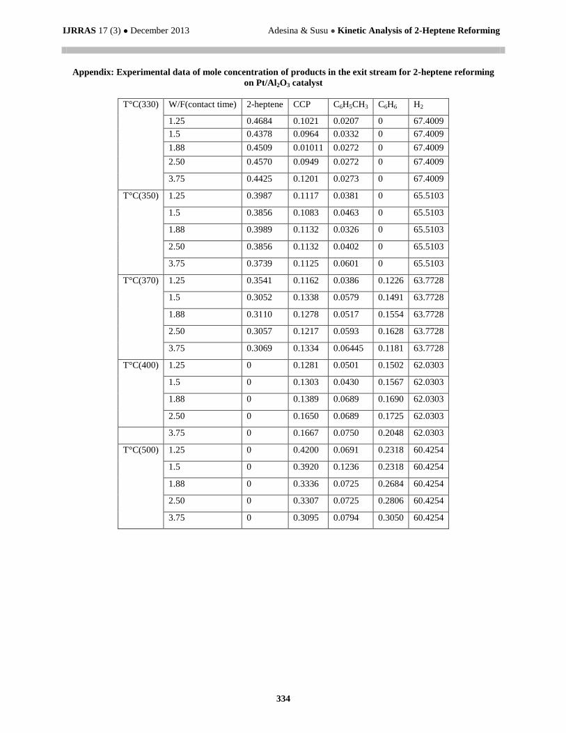
Appendix: Experimental data of mole concentration of products in the exit stream for 2-heptene reforming

on Pt/Al2O3 catalyst

T°C(330) W/F(contact time) 2-heptene CCP C6H5CH3 C6H6 H2

1.25 0.4684 0.1021 0.0207 0 67.4009

1.5 0.4378 0.0964 0.0332 0 67.4009

1.88 0.4509 0.01011 0.0272 0 67.4009

2.50 0.4570 0.0949 0.0272 0 67.4009

3.75 0.4425 0.1201 0.0273 0 67.4009

T°C(350) 1.25 0.3987 0.1117 0.0381 0 65.5103

1.5 0.3856 0.1083 0.0463 0 65.5103

1.88 0.3989 0.1132 0.0326 0 65.5103

2.50 0.3856 0.1132 0.0402 0 65.5103

3.75 0.3739 0.1125 0.0601 0 65.5103

T°C(370) 1.25 0.3541 0.1162 0.0386 0.1226 63.7728

1.5 0.3052 0.1338 0.0579 0.1491 63.7728

1.88 0.3110 0.1278 0.0517 0.1554 63.7728

2.50 0.3057 0.1217 0.0593 0.1628 63.7728

3.75 0.3069 0.1334 0.06445 0.1181 63.7728

T°C(400) 1.25 0 0.1281 0.0501 0.1502 62.0303

1.5 0 0.1303 0.0430 0.1567 62.0303

1.88 0 0.1389 0.0689 0.1690 62.0303

2.50 0 0.1650 0.0689 0.1725 62.0303

3.75 0 0.1667 0.0750 0.2048 62.0303

T°C(500) 1.25 0 0.4200 0.0691 0.2318 60.4254

1.5 0 0.3920 0.1236 0.2318 60.4254

1.88 0 0.3336 0.0725 0.2684 60.4254

2.50 0 0.3307 0.0725 0.2806 60.4254

3.75 0 0.3095 0.0794 0.3050 60.4254

kinetic analysis of 2-heptene reforming on … · ijrras 17 (3) december 2013 adesina & susu...

Documents