Seediscussions,stats,andauthorprofilesforthispublicationat:https://www.researchgate.net/publication/285597647

KinematicOptimisationofanArticulatedTruckIndependentFrontSuspensionbyUsingResponseSurface...

ConferencePaper·November2015

CITATION

1

READS

249

4authors,including:

Someoftheauthorsofthispublicationarealsoworkingontheserelatedprojects:

ComputerAidedDesignandAnalysisofaDoubleWishboneSuspensionforHeavyCommercial

VehiclesViewproject

MehmetMuratTopaç

DokuzEylulUniversity

17PUBLICATIONS63CITATIONS

SEEPROFILE

EgemenBahar

DokuzEylulUniversity

3PUBLICATIONS2CITATIONS

SEEPROFILE

AllcontentfollowingthispagewasuploadedbyMehmetMuratTopaçon04December2015.

Theuserhasrequestedenhancementofthedownloadedfile.Allin-textreferencesunderlinedinblueareaddedtotheoriginaldocumentandarelinkedtopublicationsonResearchGate,lettingyouaccessandreadthemimmediately.

KINEMATIC OPTIMISATION OF AN ARTICULATED TRUCK INDEPENDENT FRONT SUSPENSION BY USING RESPONSE SURFACE METHODOLOGY

MEHMET MURAT TOPAÇ1, EGEMEN BAHAR2,3, CAN OLGUNER2,3, NUSRET SEFA KURALAY1,

1 Dokuz Eylül University, Department of Mechanical Engineering, İzmir-TURKEY 2 Ege Endüstri ve Ticaret A.Ş., İzmir-TURKEY 3 Dokuz Eylül University, The Graduate School of Natural and Applied Sciences, İzmir-TURKEY

Abstract Conceptual kinematic design study of a double wishbone suspension that will be used as the front axle of a 40 metric tonnes capacity articulated heavy commercial vehicle is summarised. Design problem is basically established on two main goals namely, minimum deviations of the wheel track and the camber angle under all drive and load conditions. In the light of the design constraints such as the ground clearance of the tractor, chassis location, structural elements of the wheel-end package and the steel wheel, the possible design volume of the suspension was predicted. Subsequently a primary kinematic model of the suspension was built via Adams/Car™ multibody dynamics (MBD) software and the deviation characteristics of this model were computed in case of wheel jounce and rebound. Targeted optimal ranges of the kinematic parameters during the wheel travel were also obtained by using response surface methodology (RSM). For this purpose, a central composite design (CCD) - based multiobjective optimisation process was performed to the primary model by using Adams/Insight™ tool of MSC.Adams® commercial software. 3D plots of the kinematic parameters including the effects of the wheel travel and wheel steering are presented for primary and optimised designs. Results showed that the optimal geometry of the double wishbone suspension obtained from the multiobjective optimisation study satisfies the track change limitation given in the literature. Keywords: Independent front suspension (IFS), Design of experiments (DOE), Multibody dynamics (MBD), Multi-objective

optimisation, Kinematic optimisation, Central composite design (CCD)

1. INTRODUCTION

Through their high loading capacity and ease of manufacturing, solid axles have a broad application area as heavy

commercial vehicle suspension. Moreover, constant track and camber requirements have a much greater priority for

commercial vehicles than for passenger cars due to the minimisation of tyre wear, rolling resistance and fuel consumption

(Bramberger and Eichlseder, 1998 p.1). These targets can be highly attained via solid axle designs. An example of this system

can be seen in Figure 1.a (Topaç et al., 2011 p.149). On the other hand, solid axles have higher unsprung mass in comparison

with the independent suspensions. High unsprung mass affects the ride comfort, wheel-road contact and handling dynamics

adversely (Gillespie, 1992 p.165), (Gysen et al., 2010 p.1159). In addition, this may cause structural noise problems. As a

result of the comfort and control requirements, one of the main targets to be reached at the end of the design process of a

vehicle suspension is to keep the unsprung mass as small as possible. In order to satisfy these requirements, independent

suspensions are chosen as front suspensions of busses and trucks by the heavy commercial vehicle manufacturers

increasingly (Timoney and Timoney, 2003 p.426). Applied sample of the truck IFS which was designed in the scope of this

study is seen in Figure 1.b. These systems also have some advantages such as little space requirement, easier steerability, low

weight and no mutual wheel influence which are important for good road-holding characteristics. Aforementioned

advantages are most easily achieved by using double wishbone suspension (Reimpell et al., 2001 p.7). On the other hand,

kinematic characteristics of the suspension should also be taken into account during the design process. For instance,

variation range of the track change during the vertical wheel travel should not be higher than certain design limits. Deviation

characteristic of the IFS kinematic parameters during the wheel travel is highly dependent on the hardpoint positions.

Essentially, kinematic design of the independent suspension mechanism is determination of the hardpoint positions (Hwang

et al., 2007 p.1).

Elastic bushing

(Vehicle body mounting)

Air spring

Anti-roll bar

Elastic bushing

(Axle beam mounting)

Axle beam IIη

IIε

IIξ

Direction of travel

Control arm

Direction of travel Lower wishbone

Wheel-end

Spring

Upper wishbone

Kingpin

Knuckle

Connection element for spring

a. b.

Figure 1.a. Solid front axle (Topaç et al., 2011 p.149) b. Double wishbone IFS designed for articulated trucks

In this work, optimal kinematic design study of a double wishbone suspension that will be used as 7100 kg capacity front

axle of a 40 metric tonnes articulated truck was carried out by using multibody dynamics (MBD). In order to do that,

hardpoint positions of the front axle which give optimal variation range of the kinematic parameters during the wheel travel

were determined via multiobjective optimisation. Firstly, physical design limitations were determined by taking the structure

of the vehicle into account. By this way, a primary kinematic model of the IFS was built. By using the initial hardpoint

positions, a multibody model of the mechanism was performed by using MSC. Adams™ commercial software. Variation of the

kinematic parameters such as camber (σ), track (sRV) and kingpin inclination angle (δ) were computed for parallel wheel travel

and steering. After that, structural design constraints which constitute the possible design volume of the suspension

mechanism were determined. The possible ranges of a hardpoint positions were determined by taking the design limitations

such as the ground clearance, roll centre height, structural elements of the wheel-end package etc. into account. With the

use of these limitations, a Design of Experiments-Response Surface Methodology (DOE-RSM) -based optimisation study was

carried out via Adams/Insight™ multi-objective optimisation tool. By this way, optimal hardpoint locations which satisfy the

design targets namely, minimum deviations of σ and sRV during the wheel travel were obtained.

2. KINEMATIC DESCRIPTION OF THE IFS

General view and the kinematic parameters of the double wishbone suspension are seen in Figure 2.a. Here, OV is the

midpoint of the front track. In this model, double wishbone suspension is basically represented via 8 hardpoints, A1 to A8. The

points A11 and A12 also give the axis of the suspension spring. Knuckle is in connection with the upper and lower wishbones

via A3 and A4 spherical joints. A3-A4 line represents the geometric steering axis. A7 is the intersection point of steering axis and

wheel rotation axis that is described by the unit vector {eYR}. The unit vector {eL} represents the steering axis. Wishbones are

mounted to the vehicle body via bearings A1, A2, A5 and A6 which can be considered as revolute joints. Axes of the hard points

A1, A2, A5 and A6 which are mounted on a sub frame are parallel to ξ; the longitudinal axis of the vehicle. Figure 2.b also

shows the kinematic model of the double wishbone suspension. Reference frame ξ-η-ε (frame 1) is defined at the centre of

the mass SA of the vehicle body. In this model, U-V-W frame (frame 2) was also defined for each wishbone where subscripts O

and U indicate upper and lower wishbones respectively. It can be assumed that A3 and A4 rotate around the points OU and OO

which are at the origin of the U-V-W frames. Here, the unit vectors {eUU} and {eUO} also represent the rotation axes of the

wishbones. Hardpoints A9 and A10 represent the tie rod. Tie rod and knuckle are connected via A9 ball joint. Steer angle of the

wheel, βL (Figure 3.a) is adjusted by the position of A10. Position vector of A3 can be written in terms of U-V-W frame as:

VU3U1/23A eAOR (1)

As a result of the vertical wheel displacement εA8, {RA3'}2/1 can also be expressed in terms of ξ-η-ε frame as:

1/2'3A121/1OU1/1'3A RTRR (2)

where, the sign ' indicates the displaced position of the hardpoint.

A11

A12

nS

S F

Subframe

A4

A3

IIξ IIη

IIε

Direction

A8

A1

A2 A9

Symmetry

plane

Suspension spring

A5

A6

sRV

S: Steering axis - road surface intersection

F: Tyre contact patch

{eYR}

rδ

RD

Steering axis

OV

nS

A2

A4

A5

A6

A1

A3

OO

OU

A8

{eVO}

{eUU}

{eUO}

A9

{eVU} {RA3}2/1

ε

ξ η

SA

{ROU}1/1

{eYR}

A7

Direction

A10

{eL}

+εA8

-εA8

a. b.

Figure 2.a. Schematic of the truck IFS model b. Kinematic model of the IFS

Here, [T2]1 is also defined as the transformation matrix between U-V-W and ξ-η-ε frames. Position of A4 can be obtained

from the solution of the following constraint equations (Kuralay, 1985 p.19), (Simionescu and Beale, 2002 p.818), (Hwang et

al., 2007 p.2):

24A3A2

4A3A2

4A3A2

'3A2

'3A2

'3A (3)

VO4O2

OO2

OO2

OO eAO (4)

By using the same notation, new positions of A7, A8 and A9 can be computed. Camber angle and track variations caused by

the wheel displacement εA8 are shown in Figure 3.b (Topaç, 2010 p.47), (Topaç et al., 2010 p.10).

G

IIξ

δ

S´

+ σ

rδ

S

B

F

C

D

Yönlendirme ekseni

Y1

{eYR} H

sRV

Z1

X1

Hareket yönü

C

D

Z1

nS

P´

εR

Direction

IIξ

IIη

A5

A6

A3

A4

A1

A2

A8

βV

{eYR} G

A7

σ: Kamber açısı rδ: Yön verme yarıçapı nS: Kaster mesafesi βV: Ön iz açısı δ: Dingil pimi açısı εR: Kaster açısı sRV: İz genişliği βL: Yönlendirme açısı

βL

{eL}

P´

A8'

A7 A8

A1 A3

A5 A4

Δσ A4'

A3'

εA8

ε

η SA

wO

vO

YR

ZR

vU

wU

ZR'

A7' YR'

F

F´

ΔsRV / 2

uO

uU

Sym

met

ry a

xis

sRV / 2 OV

a. b.

Figure 3.a. Steer and toe angles of the wheel b. Camber and track change of a bus IFS during the jounce motion of the wheel

(Topaç et al. 2010 p.10)

Here, the displaced positions of the points A7 and A8 are shortly denoted as A7' and A8'. In order to determine the change

in i.e., camber angle, the new positions A7' and A8' can be compared with the initial positions A7 and A8. Hence the camber

change can be written as the angle Δσ between the projection of A7A8 and A7'A8' onto the ηε plane that is assumed as global

frame as:

'8A'7A8A7A

'8A'7A18A7A

RR

RRcos (5)

Kinematic parameters δ, εR and βV can also be represented by using the same formulation (Blundell and Harty, 2006 p.43).

Moreover, by using the ξ and η co-ordinates of the points F and S which are given in Figure 4, the scrub radius, rδ and the

caster arm, nS can be written respectively as (Kuralay, 1985 p.28):

SFr (6)

SFSn (7)

3. MULTIBODY MODEL

Although a parallel arm mechanism satisfies the design targets such as minimum deviations of σ and sRV in jounce and

rebound modes of the wheel, this design configuration is not applicable in many cases because of the design constraints.

Figure 4.a shows the produced final prototype of the IFS which was designed in the scope of this study. Figure 4.b also

summarises some of the design limitations which were used for the kinematic design and optimisation phases. Initial

positions of the hardpoints A3 and A4 were selected in the light of the design constraints such as the brake system, steel

wheel, steering knuckle and connection element for the suspension spring. Moreover, the effective distance c between A3

and A4 should be as large as possible to achieve small reaction forces in the link bearings and to limit the deformation of the

rubber elements fitted (Reimpell et al., 2001 p.7). Primary positions of A1 and A5 were selected by considering the chassis

position, design of the subframe, ground clearance of the vehicle and the roll centre height of the front axle. It is known from

the literature that the roll centre of a double wishbone suspension should be as low as possible to obtain minimum

deviations of σ and sRV during the wheel travel (Reimpell, 1988 p.206), (Reimpell, 2001 p.156).

A1

A2

A3

A4

A5

A6

A11

Steel wheel

A3

c

A4

Brake system

Knuckle

Design area for A3

Design area for A4

a. b.

Figure 4.a. Produced prototype of the truck IFS b. Design limitations for upper and lower control arm joints

By using the selected initial hardpoint positions, a three dimensional multibody model of the draft suspension design was

composed by using Adams/Car™ module of MSC. Adams™ as shown in Figure 5.a. In this model, the structural elements

namely, upper and lower wishbones, knuckle arm and tie rod were assumed as rigid. For the pre-load of the suspension

spring used in this model, total sprung load of the 7 metric tonnes loading capacity front axle was calculated in static loading

condition by using the equation:

gmmgmP USS (N) (8)

Here, mS is sprung mass per front wheel. m is total mass that is carried by a single wheel. Unsprung mass per wheel of the

front axle which includes wheel-end, brake system and tyre is assumed as mU ≈250 kg. In this design, suspension spring is

directly mounted to the kingpin via a revolute joint (Figure 4). By this was spring rate of the suspension can be assumed as

iF≈1 (Matschinsky, 2007 p.96,97), (Blundell and Harty, 2006 p.228-231). Upper and lower wishbones of the truck suspension

are also connected to the vehicle body via elastic bushings at A1, A2, A5 and A6 hardpoints. It is known from the literature that

elastic bushings affect the variation range of the kinematic properties of the suspension and the dynamics of the vehicle

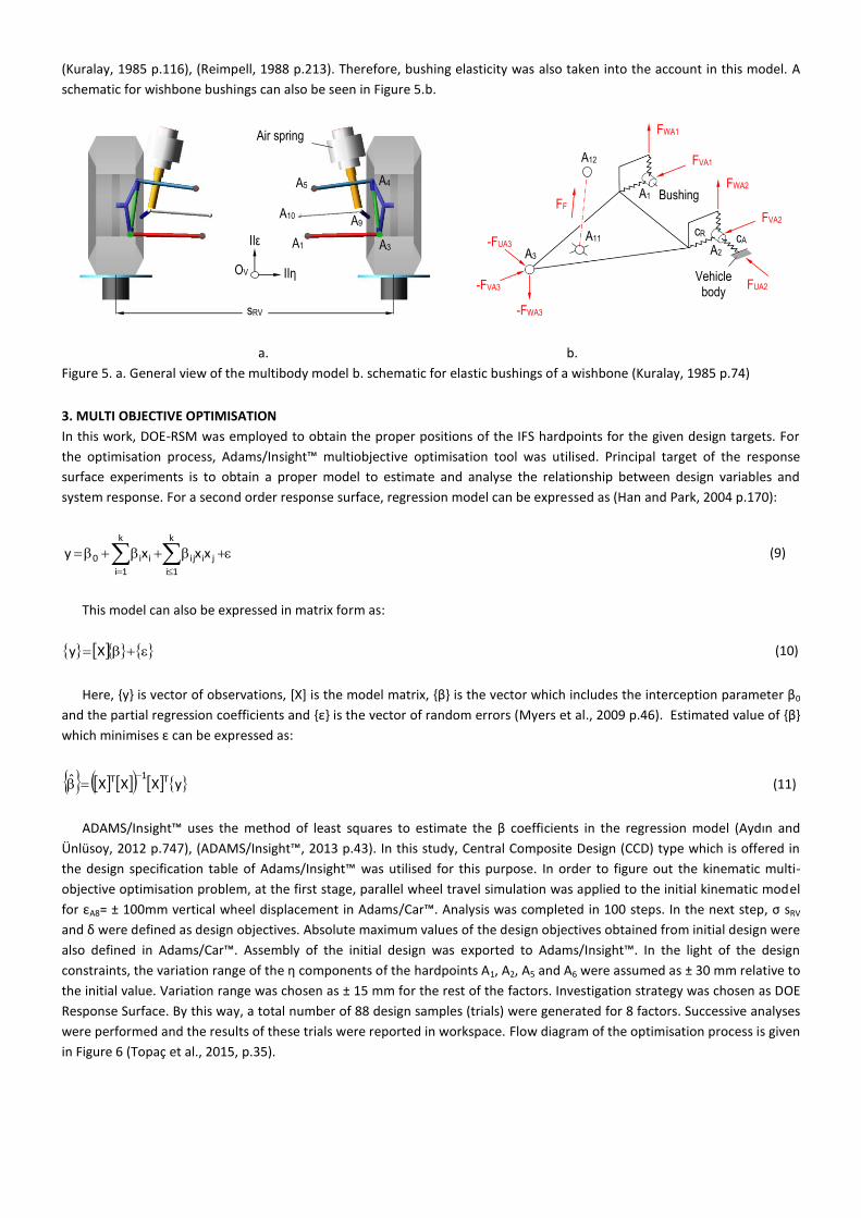
(Kuralay, 1985 p.116), (Reimpell, 1988 p.213). Therefore, bushing elasticity was also taken into the account in this model. A

schematic for wishbone bushings can also be seen in Figure 5.b.

Air spring

A1

A5

A3

A4

A9 A10

IIη

IIε

OV

sRV

cA

FF

A3

A1

A2

A11

A12

-FUA3

-FVA3

-FWA3

FWA1

FVA1

FWA2

cR

FUA2 Vehicle

body

Bushing

FVA2

a. b.

Figure 5. a. General view of the multibody model b. schematic for elastic bushings of a wishbone (Kuralay, 1985 p.74)

3. MULTI OBJECTIVE OPTIMISATION

In this work, DOE-RSM was employed to obtain the proper positions of the IFS hardpoints for the given design targets. For

the optimisation process, Adams/Insight™ multiobjective optimisation tool was utilised. Principal target of the response

surface experiments is to obtain a proper model to estimate and analyse the relationship between design variables and

system response. For a second order response surface, regression model can be expressed as (Han and Park, 2004 p.170):

k

1i

jiij

k

1i

ii0 xxxy (9)

This model can also be expressed in matrix form as:

Xy (10)

Here, {y} is vector of observations, [X] is the model matrix, {β} is the vector which includes the interception parameter β0

and the partial regression coefficients and {ε} is the vector of random errors (Myers et al., 2009 p.46). Estimated value of {β}

which minimises ε can be expressed as:

yXXXˆ T1T (11)

ADAMS/Insight™ uses the method of least squares to estimate the β coefficients in the regression model (Aydın and

Ünlüsoy, 2012 p.747), (ADAMS/Insight™, 2013 p.43). In this study, Central Composite Design (CCD) type which is offered in

the design specification table of Adams/Insight™ was utilised for this purpose. In order to figure out the kinematic multi-

objective optimisation problem, at the first stage, parallel wheel travel simulation was applied to the initial kinematic model

for εA8= ± 100mm vertical wheel displacement in Adams/Car™. Analysis was completed in 100 steps. In the next step, σ sRV

and δ were defined as design objectives. Absolute maximum values of the design objectives obtained from initial design were

also defined in Adams/Car™. Assembly of the initial design was exported to Adams/Insight™. In the light of the design

constraints, the variation range of the η components of the hardpoints A1, A2, A5 and A6 were assumed as ± 30 mm relative to

the initial value. Variation range was chosen as ± 15 mm for the rest of the factors. Investigation strategy was chosen as DOE

Response Surface. By this way, a total number of 88 design samples (trials) were generated for 8 factors. Successive analyses

were performed and the results of these trials were reported in workspace. Flow diagram of the optimisation process is given

in Figure 6 (Topaç et al., 2015, p.35).

Yes No

Converge ? (Y, N)

Converge?

Regression

Design target (Minimum Δσ,

ΔsRV …)

Design space (Generation of design trials)

OUTPUT

Adams/CarTM

1. Analyse the initial model 2. Define the design objectives (σ, δ, …)

Factors

(A1, A2, A3, …)

Analysis of design trials

Max. absolute values of the

objectives

Adams/InsightTM

1. Call the factors 2. Select design limits 3. Define targets 4. Select the investigation

strategy (e.g. DOE-RSM)

Design matrix

(Workspace)

Figure 6. Flow diagram of Adams/Insight™ kinematic optimisation process (Topaç et al., 2015, p.35)

4. RESULTS AND DISCUSSION

4.1. Optimisation of camber and track alterations

Histograms shown in Figure 7 were generated by using the results provided from the workspace. These diagrams present the

dissipation of the design points for the various values of the kinematic parameters, namely, σ, sRV and δ. Diagrams give the

number of design samples for a certain value of a parameter. Main effect plots for σ, sRV and δ are also seen in Figure 8. In

the light of the design limitations, suspension geometry which gives minimum variation of σ and sRV during jounce and

rebound was chosen by the software among the design samples.

42

35

28

21

14

7

0

27

18

9

0

Num

ber

of o

ccur

ence

s

0 0.5 0.9 1.4 1.8 2.3 2.7 3.2 3.6 4.1 4.5

Camber, σ(º)

16 18 20 21 23 25 27 29 30 32 34

Track change, ΔsRV (mm)

3 4 5 6 7 8 9 10 11 12 13

Kingpin, δ (º)

27

18

9

0

a. b. c.

Figure 7. Histograms for kinematic parameters: a. Camber b. Track c. Kingpin

Parallel wheel travel simulation for εA8= ± 100mm and steering simulation for βL= ± 50° were applied to the optimised

MBD model simultaneously. These simulations are also illustrated by using the solid model of the IFS in Figure 9. Results were

generated via Adams/PostProcessor™. Camber deviation ranges for εA8= ± 100 mm and βL= 0° were obtained for original and

optimised designs as (–2.6°; +1.8°) and (–1.8°; 1.3°) respectively. It is known from the literature that total track variation ΔsRV

of an IFS should not be higher than 25 mm for εA8= ± 40mm (Reimpell, 1976 p.149, 150). ΔsRV was calculated as 42 mm for the

primary design and 25 mm for the optimised design as seen in Figure 10. In order to improve the ease of the steerability,

variation of the kingpin inclination angle and the scrub radius are also reduced. 3D response plots obtained from MATLAB®

are also given in Figure 11.a and 11.b. Here, the comparisons of the camber angle and kingpin angle variations for initial and

optimised designs are presented as functions of εA8 and βL.

The main kinematic parameter that affects the roll dynamics of the vehicle body is the roll centre height, hMV.

Determination of hMV is given in Figure 11.a. Roll centre of the optimised design was obtained as hMV ≈ 58 mm at εA8=0 mm as

seen in Figure 11.b. Results of the multibody analyses indicated that reducing the hM decreases the variation of σ and sRV

which satisfies the design targets. However, lower hMV also increases the roll moment and the roll angle ψ of the vehicle body

during a cornering manoeuvre.

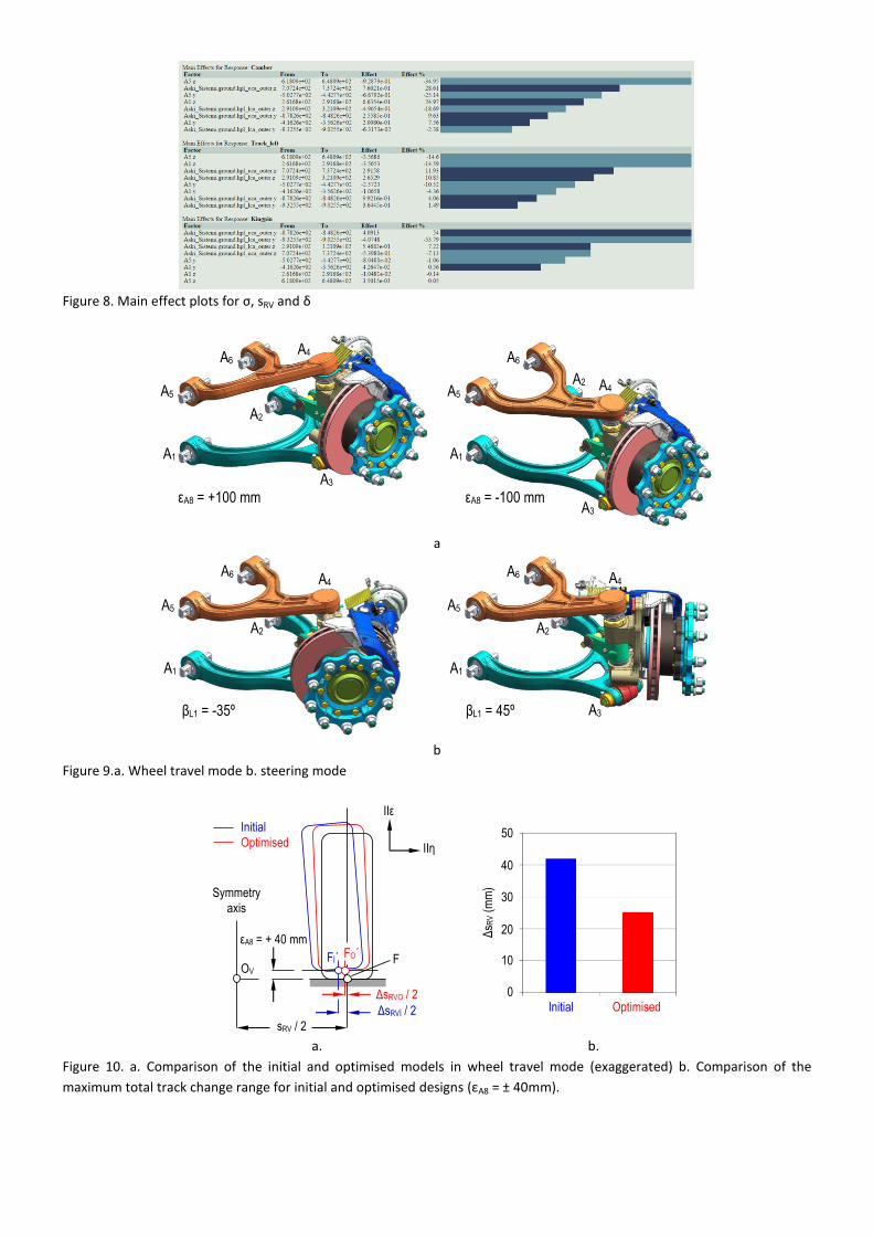
Figure 8. Main effect plots for σ, sRV and δ

a

45/35 b

εA8 = +100 mm εA8 = -100 mm

A1

A2

A3

A4

A5

A6

A1

A2 A5

A6

A3

A4

βL1 = -35º βL1 = 45º

A1

A2

A5

A6 A4

A1

A2

A5

A6 A4

A3

a

a

45/35 b

εA8 = +100 mm εA8 = -100 mm

A1

A2

A3

A4

A5

A6

A1

A2 A5

A6

A3

A4

βL1 = -35º βL1 = 45º

A1

A2

A5

A6 A4

A1

A2

A5

A6 A4

A3

b

Figure 9.a. Wheel travel mode b. steering mode

OV

IIε

IIη

sRV / 2

Symmetry

axis

ΔsRVİ / 2

ΔsRVO / 2

F

εA8 = + 40 mm

Fİ´ FO´

Initial

Optimised

50

40

30

20

10

0

Initial Optimised

Δs R

V (

mm

)

a. b.

Figure 10. a. Comparison of the initial and optimised models in wheel travel mode (exaggerated) b. Comparison of the

maximum total track change range for initial and optimised designs (εA8 = ± 40mm).

σ (º)

4

2 0

-2

ε A8

(mm

)

50

-50

0

βL (º)

100

50

0

-50

-100

εA8 (mm)

Initial

Optimised

50 0 -50

Initial design

βL (º)

Optimised design

-100

-50

0

50

100

-100

-50

0

50

100

σ (º)

4

3

2

1

0

-1

-2

-3

βL (º)

50 0 -50

a

100

50

0

-50

100

11

10

9

8

7

6

5

50

δ (º)

-50

50

0

βL (º)

-100

-50

0

100

εA8 (mm)

Optimised

Initial

Initial design

Optimised design

ε A8

(mm

)

-50 0 50

βL (º)

100

50

0

-50

-100

σ (º)

βL (º)

-50 0 50

10.5

9.5 8.5

7.5

6.5

5.5

b

Figure 11. Response surfaces for a. camber angle b. kingpin angle

OV

MV

A1

δ

J

F

P1

Chassis

K

IIε

IIη

S

rδ

sRV / 2

α

c

h

hMV

Design volume for air spring

Symmetry axis

Subframe

MV Roll centre P1 Instant centre OV Reference point h Ground clearance

Road surface

A3

A4

A5

Whe

el tr

avel

, εA

8 (m

m)

-100 -50 0 50 100 150 200 250

Roll centre height, hMV (mm)

100

50

0

-50

-100

Initial Optimised

a. b.

Figure 12.a. Determination of the roll centre b. Roll centre height deviations for initial and optimised kinematic models

4.2. Minimisation of toe deviation

One of the main targets in the kinematic design of the independent front suspensions is to minimise the βV (Figure 3.a)

variation during the service. By this way uncontrolled steering effects can be prevented. In order to do that, angular position

of the tie rod (A9-A10) should be determined with sufficient accuracy. Figure 13.a summarises the kinematic requirement to

adjust the appropriate tie rod position (Reimpell, 1974 p.150). In this study, the correct position of the hardpoint A9 for the

initial design is determined by using this principle. First, the instant centre P1 was assigned by using the positions of A2, A3, A4

and A6. Extension of the path A9-A10 should also intersect P1. α is the angle between A4-P1 and A3-P1 lines. The instant centre

P2 was also determined by using A2, A3, A4 and A6 as seen in Figure 13.Then the third instant centre P3 was found by using the

extension of the lines A6-A10 and P1-P3. Here, the angle between P1-P2 and P1-P3 lines should be equal to α. Finally, the correct

position of the hardpoint A9 was found where the extensions of A10-P1 and the extension of A4-P3 intersect. Figure 13.b also

shows the toe angle variation during jounce and rebound. For the final kinematic design, the calculated variation range of βV

is (–0.02°; +0.02°).

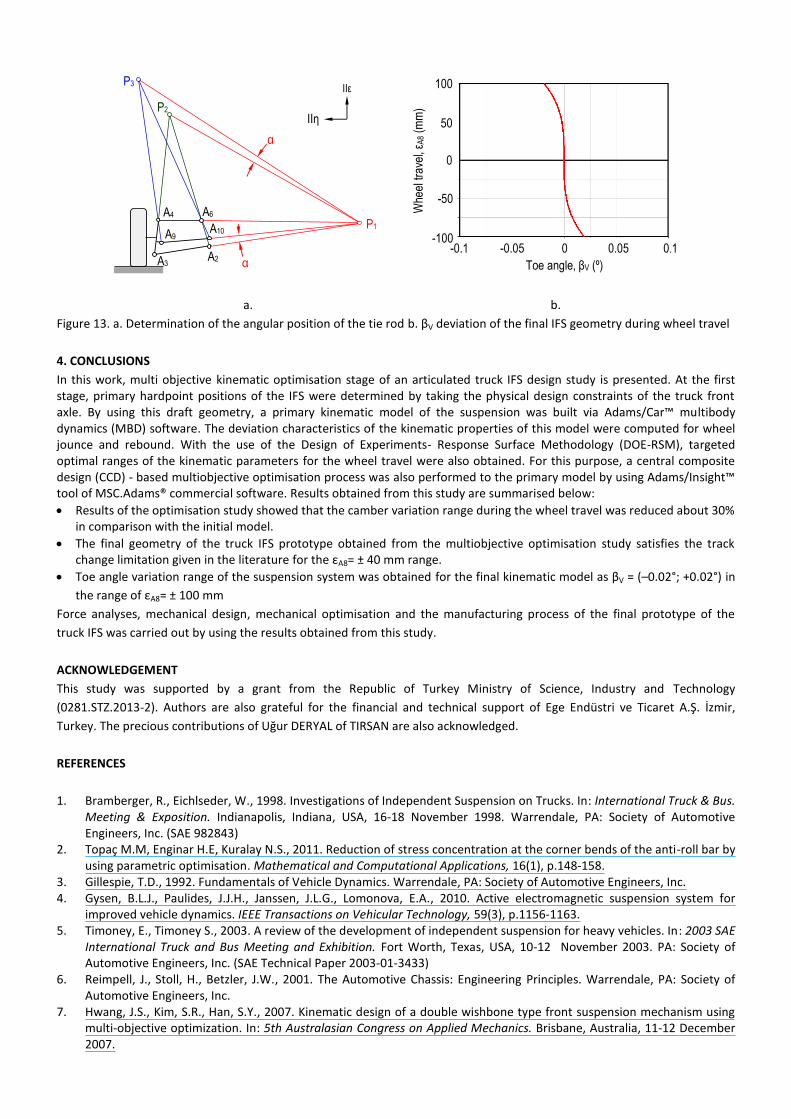
A6 A4

A3

A9

P3

P2

A2

A10 P1

α

α

IIη

IIε

Whe

el tr

avel

, εA

8 (m

m)

-0.1 -0.05 0 0.05 0.1

Toe angle, βV (º)

100

50

0

-50

-100

a. b.

Figure 13. a. Determination of the angular position of the tie rod b. βV deviation of the final IFS geometry during wheel travel

4. CONCLUSIONS

In this work, multi objective kinematic optimisation stage of an articulated truck IFS design study is presented. At the first stage, primary hardpoint positions of the IFS were determined by taking the physical design constraints of the truck front axle. By using this draft geometry, a primary kinematic model of the suspension was built via Adams/Car™ multibody dynamics (MBD) software. The deviation characteristics of the kinematic properties of this model were computed for wheel jounce and rebound. With the use of the Design of Experiments- Response Surface Methodology (DOE-RSM), targeted optimal ranges of the kinematic parameters for the wheel travel were also obtained. For this purpose, a central composite design (CCD) - based multiobjective optimisation process was also performed to the primary model by using Adams/Insight™ tool of MSC.Adams® commercial software. Results obtained from this study are summarised below:

Results of the optimisation study showed that the camber variation range during the wheel travel was reduced about 30% in comparison with the initial model.

The final geometry of the truck IFS prototype obtained from the multiobjective optimisation study satisfies the track change limitation given in the literature for the εA8= ± 40 mm range.

Toe angle variation range of the suspension system was obtained for the final kinematic model as βV = (–0.02°; +0.02°) in

the range of εA8= ± 100 mm

Force analyses, mechanical design, mechanical optimisation and the manufacturing process of the final prototype of the

truck IFS was carried out by using the results obtained from this study.

ACKNOWLEDGEMENT

This study was supported by a grant from the Republic of Turkey Ministry of Science, Industry and Technology

(0281.STZ.2013-2). Authors are also grateful for the financial and technical support of Ege Endüstri ve Ticaret A.Ş. İzmir,

Turkey. The precious contributions of Uğur DERYAL of TIRSAN are also acknowledged.

REFERENCES

1. Bramberger, R., Eichlseder, W., 1998. Investigations of Independent Suspension on Trucks. In: International Truck & Bus. Meeting & Exposition. Indianapolis, Indiana, USA, 16-18 November 1998. Warrendale, PA: Society of Automotive Engineers, Inc. (SAE 982843)

2. Topaç M.M, Enginar H.E, Kuralay N.S., 2011. Reduction of stress concentration at the corner bends of the anti-roll bar by using parametric optimisation. Mathematical and Computational Applications, 16(1), p.148-158.

3. Gillespie, T.D., 1992. Fundamentals of Vehicle Dynamics. Warrendale, PA: Society of Automotive Engineers, Inc. 4. Gysen, B.L.J., Paulides, J.J.H., Janssen, J.L.G., Lomonova, E.A., 2010. Active electromagnetic suspension system for

improved vehicle dynamics. IEEE Transactions on Vehicular Technology, 59(3), p.1156-1163. 5. Timoney, E., Timoney S., 2003. A review of the development of independent suspension for heavy vehicles. In: 2003 SAE

International Truck and Bus Meeting and Exhibition. Fort Worth, Texas, USA, 10-12 November 2003. PA: Society of Automotive Engineers, Inc. (SAE Technical Paper 2003-01-3433)

6. Reimpell, J., Stoll, H., Betzler, J.W., 2001. The Automotive Chassis: Engineering Principles. Warrendale, PA: Society of Automotive Engineers, Inc.

7. Hwang, J.S., Kim, S.R., Han, S.Y., 2007. Kinematic design of a double wishbone type front suspension mechanism using multi-objective optimization. In: 5th Australasian Congress on Applied Mechanics. Brisbane, Australia, 11-12 December 2007.

8. Kuralay, N.S., 1985. Einfluβ von Fahrwerkelastizitäten und Reifenparametern auf das Fahrverhalten von Personenkraftwagen. Ph. D. Universität Hannover.

9. Simionescu, P.A., Beale, D., 2002. Synthesis and analysis of the five-link rear suspension system used in automobiles. Mechanism and Machine Theory, 37(9), p.815-832.

10. Topaç, M.M., 2010. Numerical analysis of the influence of torsen differential on vehicle handling dynamics by using a mathematical vehicle model. Ph. D. Dokuz Eylül University.

11. Topaç, M.M., Özdel, S., Kuralay, N.S., 2010. Computer aided position analysis of a double wishbone suspension. Engineer and Machinery, 51(604), p.9-21. (in Turkish with an abstract in English).

12. Blundell, M., Harty, D., 2006. The Multibody Systems Approach to Vehicle Dynamics. London: Elsevier Butterworth – Heinemann.

13. Reimpell, J., 1988. Fahrwerktechnik: Radaufhängungen. 2nd ed. Würzburg: Vogel Buchverlag. 14. Matschinsky, W., 2007. Radführungen der Straβenfahrzeuge. 3rd ed. Berlin Heidelberg: Springer-Verlag. 15. Han, H., Park, T., 2004. Robust optimal design of multi-body systems. Multibody system dynamics, 11(2), p.167-183. 16. Myers, R.H., Montgomery, D.C., Anderson-Cook, C.M., 2009. Response Surface Methodology, Process and Product

Optimization Using Design of Experiments, 3rd ed. Hoboken, New Jersey: John Wiley & Sons, Inc. 17. Aydın, M., Ünlüsoy, S., 2012. Optimization of suspension parameters to improve impact harshness of road vehicles. The

International Journal of Advanced Manufacturing Technology, 60(5-8), p.743–754. 18. MSC. Software Corporation, 2013. MSC.Adams®, Adams/Insight™ User Guide. 19. Topaç M.M., Duran İ., Kuralay N.S., 2015. Kinematic optimisation of the steering trapezoid of a 4WD vehicle by using

design of experiments approach, In: Düzce Univesity, UMAS 2015: National Engineering Studies Symposium. Düzce, Turkey, 10-12 September 2015. Düzce: Düzce University.

20. Reimpell, J., 1976. Fahrwerktechnik, Bd. 1. 3rd ed. Würzburg: Vogel-Verlag. 21. Reimpell, J., 1974. Fahrwerktechnik, Bd. 3. Würzburg: Vogel-Verlag.

View publication statsView publication stats