kernel methods fast algorithms and real life applications
TRANSCRIPT

Kernel MethodsFast Algorithms and Real Life Applications
A Thesis
Submitted For the Degree of
Doctor of Philosophy
in the Faculty of Engineering
by
S.V.N.Vishwanathan
Department of Computer Science and AutomationIndian Institute of Science
Bangalore – 560 012
JULY 2003

To my parents
for
everything . . .

Acknowledgments
They say that once in your lifetime there comes a person who opens the doors of your mind and
makes you more aware of yourself. For me such a person has been Prof. M.Narasimha Murty.
More than being my thesis adviser, he has been a friend, philosopher and guide in the truest
sense. Every time I had a problem, personal or professional, I rushed to him for advise, and
he never ever let me down. His immense confidence in me allowed me to achieve goals much
beyond my capabilities. I attribute whatever technical sophistication that can be found in this
thesis to his inspiration, motivation and guidance.
Whatever I thought were the qualities of a world class researcher and a good human being,
I found much more than that in Dr. Alexander Smola. His energy and enthusiasm for research
and his ability to listen to my endless ramblings and most importantly his belief in me have
contributed immensely to this thesis. I must thank Miki for patiently bearing with me when
I kept Alex at his office for long hours or discussed kernel methods with him on the way to
Mysore.
A part of my work was carried out at the Research School of Information Science and
Engineering (RSISE), Australian National University (ANU). I would like to thank RSISE for
an opportunity to attend the Machine Learning Summer School - 2002 and for hospitality and
facilities extended during my visit.
I would like to thank Prof. Adimurty for being very patient with me and teaching me whatever
little Analysis and Topology that I know. I would like to thank Prof. Vittal Rao for teaching
me Linear Algebra.
Many people have contributed to my education both technical and non-technical. Here I
must mention Mr. Satyam Dwivedi. He has been an near perfect room mate and a valuable
friend who has helped me gain insights into various aspects of life. My lab mates have helped
me in various ways both personal and technical. Chapter 7 was inspired by a discussion with
i

P. Viswanath.
I would like to thank the department of Computer Science and Automation for creating a
world class environment for research. Prof. Y.N. Srikant the chairman of the department has
been especially helpful in shielding me from administrivia at different stages of my Ph.D. The
office staff especially Mrs. Meenakshi, Mrs. Lalitha and Mr. Mohan have been very helpful during
the entire course of my stay at the Institute.
The research work reported in this thesis was supported by an Infosys fellowship, a travel
grant from Netscaler Inc., a grant from TriVium India Software Ltd. and a grant from the
Australian Research Council.
Finally, I want to thank my parents for everything. They taught me that dreams are im-
portant, however big or small they may be. They have been very supportive of my dream to
pursue a Ph.D. I consider myself immensely lucky to have parents like them. Although they
were physically far away from me, their immense faith in me always kept me going. I dedicate
this thesis to them.
S.V.N.Vishwanathan

Contents
Acknowledgments i
Abstract viii
1 Introduction 1
1.1 VC Theory - A Brief Primer . . . . . . . . . . . . . . . . . . . . . . . . . . . . . . 2
1.1.1 The Learning Problem . . . . . . . . . . . . . . . . . . . . . . . . . . . . . 2
1.1.2 Traditional Approach to Learning Algorithms . . . . . . . . . . . . . . . . 2
1.1.3 VC Bounds . . . . . . . . . . . . . . . . . . . . . . . . . . . . . . . . . . . 4
1.1.4 Structural Risk Minimization . . . . . . . . . . . . . . . . . . . . . . . . . 6
1.2 Introduction to Linear SVM’s . . . . . . . . . . . . . . . . . . . . . . . . . . . . . 7
1.2.1 Linear Hard-Margin Formulation . . . . . . . . . . . . . . . . . . . . . . . 8
1.2.2 Linear Soft-Margin Formulation . . . . . . . . . . . . . . . . . . . . . . . 9
1.2.3 ν-SVM Formulation . . . . . . . . . . . . . . . . . . . . . . . . . . . . . . 10
1.3 The Kernel Trick . . . . . . . . . . . . . . . . . . . . . . . . . . . . . . . . . . . . 11
1.4 Quadratic Soft-Margin Formulation . . . . . . . . . . . . . . . . . . . . . . . . . . 14
1.5 Contributions and a Road Map of this Thesis . . . . . . . . . . . . . . . . . . . . 14
1.6 Summary . . . . . . . . . . . . . . . . . . . . . . . . . . . . . . . . . . . . . . . . 16
2 SimpleSVM: A SVM Training Algorithm 17
2.1 Notation and Background . . . . . . . . . . . . . . . . . . . . . . . . . . . . . . . 18
2.2 Related Work . . . . . . . . . . . . . . . . . . . . . . . . . . . . . . . . . . . . . . 19
2.3 The Basic Idea . . . . . . . . . . . . . . . . . . . . . . . . . . . . . . . . . . . . . 20
2.4 SimpleSVM . . . . . . . . . . . . . . . . . . . . . . . . . . . . . . . . . . . . . . . 21
2.4.1 The Dual Problem . . . . . . . . . . . . . . . . . . . . . . . . . . . . . . . 22
iii

2.4.2 Finite Time Convergence . . . . . . . . . . . . . . . . . . . . . . . . . . . 22
2.4.3 Rate of Convergence . . . . . . . . . . . . . . . . . . . . . . . . . . . . . . 23
2.5 Updates . . . . . . . . . . . . . . . . . . . . . . . . . . . . . . . . . . . . . . . . . 24
2.5.1 Initialization . . . . . . . . . . . . . . . . . . . . . . . . . . . . . . . . . . 24
2.5.2 Adding a Point . . . . . . . . . . . . . . . . . . . . . . . . . . . . . . . . . 25
2.5.3 Removing a Point . . . . . . . . . . . . . . . . . . . . . . . . . . . . . . . 25
2.6 Extensions . . . . . . . . . . . . . . . . . . . . . . . . . . . . . . . . . . . . . . . . 28
2.6.1 Rank-Degenerate Kernels . . . . . . . . . . . . . . . . . . . . . . . . . . . 28
2.6.2 Linear Soft-margin Loss . . . . . . . . . . . . . . . . . . . . . . . . . . . . 29
2.7 Experiments . . . . . . . . . . . . . . . . . . . . . . . . . . . . . . . . . . . . . . . 29
2.7.1 Experimental Setup and Datasets . . . . . . . . . . . . . . . . . . . . . . . 30
2.7.2 Discussion of the Results . . . . . . . . . . . . . . . . . . . . . . . . . . . 30
2.8 Summary and Outlook . . . . . . . . . . . . . . . . . . . . . . . . . . . . . . . . . 36
3 Modified Cholesky Factorization 38
3.1 Introduction . . . . . . . . . . . . . . . . . . . . . . . . . . . . . . . . . . . . . . . 39
3.1.1 Previous Work . . . . . . . . . . . . . . . . . . . . . . . . . . . . . . . . . 39
3.1.2 Notation . . . . . . . . . . . . . . . . . . . . . . . . . . . . . . . . . . . . . 40
3.2 Matrix Factorization . . . . . . . . . . . . . . . . . . . . . . . . . . . . . . . . . . 41
3.2.1 Triangular Factors . . . . . . . . . . . . . . . . . . . . . . . . . . . . . . . 41
3.2.2 Factorization . . . . . . . . . . . . . . . . . . . . . . . . . . . . . . . . . . 42
3.2.3 Uniqueness and Existence . . . . . . . . . . . . . . . . . . . . . . . . . . . 42
3.2.4 Solution of Linear System . . . . . . . . . . . . . . . . . . . . . . . . . . . 44
3.2.5 Parallelization and Implementation Issues . . . . . . . . . . . . . . . . . . 45
3.2.6 Extensions . . . . . . . . . . . . . . . . . . . . . . . . . . . . . . . . . . . 46
3.3 An LDV Factorization . . . . . . . . . . . . . . . . . . . . . . . . . . . . . . . . . 47
3.4 Rank Modifications . . . . . . . . . . . . . . . . . . . . . . . . . . . . . . . . . . . 49
3.4.1 Generic Rank-1 Update . . . . . . . . . . . . . . . . . . . . . . . . . . . . 49
3.4.2 Rank-1 Update Where p = Z q . . . . . . . . . . . . . . . . . . . . . . . . 50
3.4.3 Removal of a Row and Column . . . . . . . . . . . . . . . . . . . . . . . . 51
3.5 Applications . . . . . . . . . . . . . . . . . . . . . . . . . . . . . . . . . . . . . . . 52
3.5.1 Interior Point Methods . . . . . . . . . . . . . . . . . . . . . . . . . . . . . 52

3.5.2 Lazy Decomposition . . . . . . . . . . . . . . . . . . . . . . . . . . . . . . 54
3.5.3 Support Vector Machines . . . . . . . . . . . . . . . . . . . . . . . . . . . 55
3.6 Summary . . . . . . . . . . . . . . . . . . . . . . . . . . . . . . . . . . . . . . . . 56
4 Kernels on Discrete Objects 57
4.1 Introduction . . . . . . . . . . . . . . . . . . . . . . . . . . . . . . . . . . . . . . . 58
4.1.1 Applications of Kernels on Discrete Structures . . . . . . . . . . . . . . . 58
4.1.2 Previous Work . . . . . . . . . . . . . . . . . . . . . . . . . . . . . . . . . 59
4.2 Defining Kernels . . . . . . . . . . . . . . . . . . . . . . . . . . . . . . . . . . . . 60
4.2.1 Haussler’s R-Convolution . . . . . . . . . . . . . . . . . . . . . . . . . . . 60
4.2.2 Exact and Inexact Matches . . . . . . . . . . . . . . . . . . . . . . . . . . 61
4.3 Sets . . . . . . . . . . . . . . . . . . . . . . . . . . . . . . . . . . . . . . . . . . . 62
4.3.1 Implementation Strategies . . . . . . . . . . . . . . . . . . . . . . . . . . . 62
4.4 Strings . . . . . . . . . . . . . . . . . . . . . . . . . . . . . . . . . . . . . . . . . . 63
4.4.1 Notation . . . . . . . . . . . . . . . . . . . . . . . . . . . . . . . . . . . . . 63
4.4.2 Various String Kernels . . . . . . . . . . . . . . . . . . . . . . . . . . . . . 64
4.5 Trees . . . . . . . . . . . . . . . . . . . . . . . . . . . . . . . . . . . . . . . . . . . 66
4.5.1 Notation . . . . . . . . . . . . . . . . . . . . . . . . . . . . . . . . . . . . . 66
4.5.2 Various Tree Kernels . . . . . . . . . . . . . . . . . . . . . . . . . . . . . . 67
4.5.3 Coarsening Levels . . . . . . . . . . . . . . . . . . . . . . . . . . . . . . . 68
4.6 Automata . . . . . . . . . . . . . . . . . . . . . . . . . . . . . . . . . . . . . . . . 69
4.6.1 Finite State Automata . . . . . . . . . . . . . . . . . . . . . . . . . . . . . 69
4.6.2 Pushdown Automata . . . . . . . . . . . . . . . . . . . . . . . . . . . . . . 71
4.7 Images . . . . . . . . . . . . . . . . . . . . . . . . . . . . . . . . . . . . . . . . . . 72
4.8 Summary . . . . . . . . . . . . . . . . . . . . . . . . . . . . . . . . . . . . . . . . 72
5 Fast String and Tree Kernels 74
5.1 Introduction . . . . . . . . . . . . . . . . . . . . . . . . . . . . . . . . . . . . . . . 75
5.2 String Kernel Definition . . . . . . . . . . . . . . . . . . . . . . . . . . . . . . . . 76
5.3 Suffix Trees . . . . . . . . . . . . . . . . . . . . . . . . . . . . . . . . . . . . . . . 77
5.3.1 Definition of a Suffix Tree . . . . . . . . . . . . . . . . . . . . . . . . . . . 77
5.3.2 The Sentinel Character . . . . . . . . . . . . . . . . . . . . . . . . . . . . 78

5.3.3 Suffix Links . . . . . . . . . . . . . . . . . . . . . . . . . . . . . . . . . . . 79
5.3.4 Efficient Construction . . . . . . . . . . . . . . . . . . . . . . . . . . . . . 79
5.3.5 Merging Suffix Trees . . . . . . . . . . . . . . . . . . . . . . . . . . . . . . 79
5.4 Algorithm for Calculating Matching Statistics . . . . . . . . . . . . . . . . . . . . 80
5.4.1 Definition of Matching Statistics . . . . . . . . . . . . . . . . . . . . . . . 80
5.4.2 Matching Statistics Algorithm . . . . . . . . . . . . . . . . . . . . . . . . 81
5.4.3 Matching Substrings . . . . . . . . . . . . . . . . . . . . . . . . . . . . . . 81
5.5 Our Algorithm for String Kernels . . . . . . . . . . . . . . . . . . . . . . . . . . . 82
5.5.1 Our Algorithm . . . . . . . . . . . . . . . . . . . . . . . . . . . . . . . . . 82
5.6 Weights and Kernels . . . . . . . . . . . . . . . . . . . . . . . . . . . . . . . . . . 85
5.7 Linear Time Prediction . . . . . . . . . . . . . . . . . . . . . . . . . . . . . . . . 86
5.8 Tree Kernels . . . . . . . . . . . . . . . . . . . . . . . . . . . . . . . . . . . . . . 87
5.8.1 Ordering Trees . . . . . . . . . . . . . . . . . . . . . . . . . . . . . . . . . 88
5.8.2 Coarsening . . . . . . . . . . . . . . . . . . . . . . . . . . . . . . . . . . . 90
5.9 Experimental Results . . . . . . . . . . . . . . . . . . . . . . . . . . . . . . . . . . 91
5.10 Summary . . . . . . . . . . . . . . . . . . . . . . . . . . . . . . . . . . . . . . . . 93
6 Kernels and Dynamic Systems 94
6.1 Introduction . . . . . . . . . . . . . . . . . . . . . . . . . . . . . . . . . . . . . . . 95
6.2 Linear Time-Invariant Systems . . . . . . . . . . . . . . . . . . . . . . . . . . . . 96
6.3 Kernels On Initial Conditions . . . . . . . . . . . . . . . . . . . . . . . . . . . . . 97
6.3.1 Discrete Time Systems . . . . . . . . . . . . . . . . . . . . . . . . . . . . . 98
6.3.2 Continuous Time Systems . . . . . . . . . . . . . . . . . . . . . . . . . . . 100
6.3.3 Special Cases . . . . . . . . . . . . . . . . . . . . . . . . . . . . . . . . . . 103
6.4 Kernels on Dynamic Systems . . . . . . . . . . . . . . . . . . . . . . . . . . . . . 104
6.4.1 Discrete Time Systems . . . . . . . . . . . . . . . . . . . . . . . . . . . . . 105
6.4.2 Continuous Time Systems . . . . . . . . . . . . . . . . . . . . . . . . . . . 106
6.4.3 Non-Homogeneous Linear Time-Invariant Systems . . . . . . . . . . . . . 108
6.5 Summary . . . . . . . . . . . . . . . . . . . . . . . . . . . . . . . . . . . . . . . . 109
7 Jigsawing: A Method to Create Virtual Examples 110
7.1 Background and Notation . . . . . . . . . . . . . . . . . . . . . . . . . . . . . . . 111
7.2 Related Work . . . . . . . . . . . . . . . . . . . . . . . . . . . . . . . . . . . . . . 112
7.3 Basic Idea . . . . . . . . . . . . . . . . . . . . . . . . . . . . . . . . . . . . . . . . 113
7.4 Jigsawing . . . . . . . . . . . . . . . . . . . . . . . . . . . . . . . . . . . . . . . . 115
7.4.1 Notation . . . . . . . . . . . . . . . . . . . . . . . . . . . . . . . . . . . . . 115
7.4.2 Algorithm . . . . . . . . . . . . . . . . . . . . . . . . . . . . . . . . . . . . 116
7.4.3 Time Complexity . . . . . . . . . . . . . . . . . . . . . . . . . . . . . . . . 116
7.4.4 Why does Jigsawing Work? . . . . . . . . . . . . . . . . . . . . . . . . . . 117
7.5 Applications . . . . . . . . . . . . . . . . . . . . . . . . . . . . . . . . . . . . . . . 118
7.6 An Image Kernel . . . . . . . . . . . . . . . . . . . . . . . . . . . . . . . . . . . . 119
7.6.1 Algorithm . . . . . . . . . . . . . . . . . . . . . . . . . . . . . . . . . . . . 119
7.6.2 Quadratic Time Prediction . . . . . . . . . . . . . . . . . . . . . . . . . . 120
7.7 Summary . . . . . . . . . . . . . . . . . . . . . . . . . . . . . . . . . . . . . . . . 121
8 Summary and Future Work 123
8.1 Contributions of the Thesis . . . . . . . . . . . . . . . . . . . . . . . . . . . . . . 123
8.2 Extensions and Future Work . . . . . . . . . . . . . . . . . . . . . . . . . . . . . 124
A Rank One Modification 126
A.1 Rank Modification of a Positive Matrix . . . . . . . . . . . . . . . . . . . . . . . 126
A.1.1 Rank One Extension . . . . . . . . . . . . . . . . . . . . . . . . . . . . . . 127
A.1.2 Rank One Reduction . . . . . . . . . . . . . . . . . . . . . . . . . . . . . . 127
A.2 Rank-Degenerate Kernels . . . . . . . . . . . . . . . . . . . . . . . . . . . . . . . 129
Bibliography 130

Abstract
Support Vector Machines (SVM) have recently gained prominence in the field of machine learning
and pattern classification (Vapnik, 1995, Herbrich, 2002, Scholkopf and Smola, 2002). Classifi-
cation is achieved by finding a separating hyperplane in a feature space which can be mapped
back onto a non-linear surface in the input space. However, training a SVM involves solving a
quadratic optimization problem, which tends to be computationally intensive. Furthermore, it
can be subject to stability problems and is non-trivial to implement. This thesis proposes a fast
iterative Support Vector training algorithm which overcomes some of these problems.
Our algorithm, which we christen SimpleSVM, works mainly for the quadratic soft margin
loss (also called the `2 formulation). We also sketch an extension for the linear soft-margin loss
(also called the `1 formulation). SimpleSVM works by incrementally changing a candidate Sup-
port Vector set using a locally greedy approach, until the supporting hyperplane is found within
a finite number of iterations. It is derived by a simple (yet computationally crucial) modification
of the incremental SVM training algorithm of Cauwenberghs and Poggio (2001) which allows us
to perform update operations very efficiently. Constant-time methods for initialization of the
algorithm and experimental evidence for the speed of the proposed algorithm, when compared to
methods such as Sequential Minimal Optimization and the Nearest Point Algorithm are given.
We present results on a variety of real life datasets to validate our claims.
In many real life applications, especially for the `2 formulation, the kernel matrix K ∈ Rn×n
can be written as
K = Z>Z + Λ,
where, Z ∈ Rn×m with m � n and Λ ∈ Rn×n is diagonal with nonnegative entries. Hence the
matrix K − Λ is rank-degenerate. Extending the work of Fine and Scheinberg (2001) and Gill
et al. (1975) we propose an efficient factorization algorithm which can be used to find a LDL>
viii
factorization ofK in O(nm2) time. The modified factorization, after a rank one update ofK, can
be computed in O(m2) time. We show how the SimpleSVM algorithm can be sped up by taking
advantage of this new factorization. We also demonstrate applications of our factorization to
interior point methods. We show a close relation between the LDV factorization of a rectangular
matrix and our LDL> factorization (Gill et al., 1975).
An important feature of SVM’s is that they can work with data from any input domain as
long as a suitable mapping into a Hilbert space can be found, in other words, given the input
data we should be able to compute a positive semi-definite kernel matrix of the data (Scholkopf
and Smola, 2002). In this thesis we propose kernels on a variety of discrete objects, such as
strings, trees, Finite State Automata, and Pushdown Automata. We show that our kernels
include as special cases the celebrated Pair-HMM kernels (Durbin et al., 1998, Watkins, 2000),
the spectrum kernel (Leslie et al., 2002a), convolution kernels for NLP (Collins and Duffy, 2001),
graph diffusion kernels (Kondor and Lafferty, 2002) and various other string-matching kernels.
Because of their widespread applications in bio-informatics and web document based algo-
rithms, string kernels are of special practical importance. By intelligently using the matching
statistics algorithm of Chang and Lawler (1994), we propose, perhaps, the first ever algorithm to
compute string kernels in linear time. This obviates dynamic programming with quadratic time
complexity and makes string kernels a viable alternative for the practitioner. We also propose
extensions of our string kernels to compute kernels on trees efficiently. This thesis presents a
linear time algorithm for ordered trees and a log-linear time algorithm for un-ordered trees.
In general, SVM’s require time proportional to the number of Support Vectors for prediction.
In case the dataset is noisy a large fraction of the data points become Support Vectors and thus
time required for prediction increases. But, in many applications like search engines or web
document retrieval, the dataset is noisy, yet, the speed of prediction is critical. We propose a
method for string kernels by which the prediction time can be reduced to linear in the length of
the sequence to be classified, regardless of the number of Support Vectors. We achieve this by
using a weighted version of our string kernel algorithm.
We explore the relationship between dynamic systems and kernels. We define kernels on var-
ious kinds of dynamic systems including Markov chains (both discrete and continuous), diffusion
processes on graphs and Markov chains, Finite State Automata, various linear time-invariant

systems etc. Trajectories are used to define kernels induced on initial conditions by the under-
lying dynamic system. The same idea is extended to define kernels on a dynamic system with
respect to a set of initial conditions. This framework leads to a large number of novel kernels
and also generalizes many previously proposed kernels.
Lack of adequate training data is a problem which plagues classifiers. We propose a new
method to generate virtual training samples in the case of handwritten digit data. Our method
uses the two dimensional suffix tree representation of a set of matrices to encode an exponential
number of virtual samples in linear space thus leading to an increase in classification accuracy.
This in turn, leads us naturally to a compact data dependent representation of a test pattern
which we call the description tree. We propose a new kernel for images and demonstrate a
quadratic time algorithm for computing it by using the suffix tree representation of an image.
We also describe a method to reduce the prediction time to quadratic in the size of the test
image by using techniques similar to those used for string kernels.

Chapter 1
Introduction
This chapter introduces our notation and presents a tutorial introduction to Support Vector
Machines (SVM). Various loss functions which give rise to slightly different quadratic optimiza-
tion problems are discussed. Intuitive arguments are provided to show the relation between
SVM’s and Structural Risk Minimization (SRM). We also try to explain why SVM’s perform so
well on a variety of challenging problems. The main contributions of this thesis are also briefly
discussed.
In Section 1.1 we present a brief introduction to VC theory. We also point out a few short-
comings of traditional machine learning algorithms and show how these lead naturally to the
development of SVM’s. In Section 1.2 we introduce the linearly separable SVM formulation.
We then discuss the linear hard-margin formulation and extend it to the linear soft-margin for-
mulation. Going further we sketch the ν-SVM formulation and briefly discuss the interpretation
of parameter ν. We also briefly touch upon the relation between the ν-SVM formulation and
the linear soft-margin formulation. In Section 1.3 we introduce the kernel trick and show how
it can be used to project points to a higher dimensional space where they may be linearly sep-
arable. The kernel trick can also be used to extend SVM’s to work with non-vectorial data. In
Section 1.4 we discuss the extension to the quadratic soft-margin loss formulation also known
as the `2 formulation. The main contributions of this thesis are presented in Section 1.5. We
conclude this chapter with a summary in Section 1.6.
The aim of this chapter is to sketch various ideas and provide an overview of basic concepts.
It tries to provide numerous references to published literature for further reading. As such, there
are no pre-requisites to read this chapter, although a basic familiarity with machine learning
1
1.1 VC Theory - A Brief Primer 2
and pattern recognition will be useful. In general we sacrifice some mathematical rigor in
order to present more intuition to the reader. Throughout this chapter we concentrate our
attention entirely on the pattern recognition problem, an excellent tutorial on the use of SVM’s
for regression can be found in Smola and Scholkopf (1998).
1.1 VC Theory - A Brief Primer
In this section we formalize the binary learning problem. We then present the traditional
approach to learning and point out some of its shortcomings. We go on to give some intuition
behind the concept of VC-dimension and show why capacity plays an important role while
designing classifiers (Vapnik, 1995).
1.1.1 The Learning Problem
In the following, we denote by {(x1, y1), . . . , (xn, yn)} ⊂ X ×{±1} the set of labeled training
samples 1, where xi are drawn from some input domain X while yi ∈ {±1}, denote the class labels
+1 and −1 respectively. Furthermore, let n be the total number of points and let n+ and n−
denote the number of points in class +1 and −1 respectively. We assume that the samples are all
drawn i.i.d (Independent and Identically Distributed) from an unknown probability distribution
P (x, y).
Let F be a class of functions f : X → {±1} parameterized by a set of adjustable parameters
ρ. For example, ρ could be the weights on various nodes of a neural network. The goal of
building learning machines is to choose a ρ such that we can predict well on unknown samples
drawn from the same underlying distribution P (x, y).
1.1.2 Traditional Approach to Learning Algorithms
The empirical error for the given training set is defined as
Eemp(ρ) =n∑
i=1
c(f(xi, ρ), yi),
1For convenience of notation, throughout this thesis, we assume that there are no duplicates in the observations.

1.1 VC Theory - A Brief Primer 3
where f(x, ρ) is the class label predicted by the algorithm and c(., .) is some error function. The
empirical risk for a learning machine is just the measured mean error rate on the training set.
Using a 0− 1 loss function it can be written as
Remp(ρ) =12n
n∑i=1
|f(xi, ρ)− yi|.
The actual risk which is the mean of the error rate on the entire distribution P (x, y) is defined
as
Ractual(ρ) =∫
12|f(xi, ρ)− yi| dP (x, y).
Since, the underlying distribution P (x, y) is not known it is generally not possible to compute
the actual risk.
Many traditional learning algorithms concentrated their energy on the task of minimizing
the empirical risk on the training samples (Haykin, 1994). The hope was that, if the training
set was sufficiently representative of the underlying distribution, the algorithm would learn the
distribution and hence generalize to make proper predictions on unknown test samples. In other
words, what we are hoping for is that the mean of the empirical risk converges to the actual
risk as the number of training points increases to infinity (Vapnik, 1995). But, researchers soon
realized that this was not always the case. For example, consider the toy 2-d classification
problem depicted in Figure 1.1. The decision function on the left is a simple one which mis-
classifies a lot of points while that on the right is quite complex and manages to drive the
empirical risk to zero. But, we intuitively expect the function in the middle, which makes a few
errors on the training set, to generalize well on unseen data points.
As another example, consider a learning algorithm that naively remembers the class label
of every training sample presented to it. Following Burges (1998), we call such an algorithm a
memory machine. The memory machine of course has 100% accuracy on the training samples,
but, clearly cannot generalize on the test set.
If F is very rich, then, for each function f ∈ F and any test set {(x1, y1), . . . , (xm, ym)} ⊂
X ×{±1} such that {x1, . . . , xm} ∩ {x1, . . . , xn} = ∅, there exists another function f∗ such that
f(xi) = f∗(xi)∀i ∈ {1, . . . , n}, while, f(xi) 6= f∗(xi)∀i ∈ {1, . . . ,m}. As we are only given the
training data, we have no means of selecting which of the two functions (and hence which of
the two different sets of test label predictions) is preferable (Scholkopf and Smola, 2002). Thus,

1.1 VC Theory - A Brief Primer 4
Figure 1.1: Three different decision functions for the same classification problem. The hollowand filled circles belong to two different classes. Error points are shown with a x. (CourtesyScholkopf and Smola (2002))
it is clear that we need some more conditions on F to make the empirical risk converge to the
actual risk. These conditions are provided by the VC bounds (Vapnik, 1995).
1.1.3 VC Bounds
Let 0 ≤ η ≤ 1 be a number. Then, Vapnik and Chervonenkis proved that, for the 0 − 1 loss
function, with probability 1− η, the following bound holds (Vapnik, 1995)
Ractual(ρ) ≤ Remp(ρ) + φ
(h
n,log(η)n
), (1.1)
where
φ
(h
n,log(η)n
)= n
√h(log(2n/h) + 1)− log(η/4)
n, (1.2)
is called the confidence term. Here h is defined to be a non negative integer called the Vapnik
Chervonenkis (VC) dimension. The VC-dimension of a machine measures the capacity of the
class F that the machine can implement. A finite set of h points is said to be shattered by F if
for each of the possible 2h labellings there is a f ∈ F which correctly classifies the points. The
VC dimension is defined as the largest h such that there exists a set of h points which the class
can shatter, and ∞ if no such h exists.
For example, consider the VC dimension of the set of hyperplanes in R2. There are 23 = 8
ways of assigning 3 points to two classes. For points shown in Figure 1.2 all 8 possibilities can
be realized using separating hyperplanes, in other words, the function class can shatter 3 points.
But, we can see that given any 4 points we cannot find hyperplanes which realize each of the

1.1 VC Theory - A Brief Primer 5
24 = 16 possible labellings. Therefore, the VC dimension of the class of separating hyperplanes
in R2 is 3.
Figure 1.2: VC dimension of the class of separating hyperplanes in R2. (Courtesy Scholkopf andSmola (2002))
Consider the memory machine that we introduced in Section 1.1.2. Clearly, this machine can
drive the empirical risk to zero, but, still does not generalize well because it has a large capacity.
This leads us to the observation that, while minimizing empirical error is important, it is equally
important to use a machine with a low capacity. In other words, given two machines with the
same empirical risk, we have higher confidence in the machine with the lower VC-dimension.
A word of caution is in order here. It is often very difficult to measure the VC-dimension of
a machine practically. As a result, it is quite difficult to calculate the VC bounds explicitly. The
bounds provided by VC theory are often very loose and may not be of practical use. Tighter
bounds are provided by the annealed VC entropy or the growth function, but, they are even
more difficult to estimate in practice. It must also be borne in mind that only an upper bound
on the actual risk is available. This does not mean that a machine with larger capacity will
always generalize poorly. What the bound says is that, given the training data, we have more
confidence in a machine which has lower capacity. In some sense Equation (1.1) is a restatement
of the celebrated principle of Occam’s razor.

1.1 VC Theory - A Brief Primer 6
1.1.4 Structural Risk Minimization
The bounds provided by VC theory can be exploited in order to do model selection. A structure
is a nested class of functions Si such that
S1 ⊆ S2 ⊆ . . . ⊆ Sn ⊆ . . .
and hence their corresponding VC-dimensions hi satisfy
h1 ≤ h2 ≤ . . . ≤ hn . . .
Now, because of the nested structure of the function classes the empirical risk Remp decreases as
we move towards a bigger class. This is because, the complexity of the function class increases
and hence it can explain the training data well. But, since the VC-dimensions are increasing
the confidence bound (φ) increases as h increases. The curves shown in Figure 1.3 depict
Equation (1.1) and the above observations pictorially.
Figure 1.3: Graphical depiction of the structural risk minimization (SRM) induction principle.(Courtesy Scholkopf and Smola (2002))

1.2 Introduction to Linear SVM’s 7
Figure 1.4: The circles and diamonds belong to two different classes. The solid line representsthe maximally separating linear boundary. Points x1 and x2 are Support Vectors. (CourtesyScholkopf and Smola (2002))
These observations suggest a principled way of selecting a class of functions. The function
class is decomposed into a nested sequence of subsets of increasing size (and thus, of increasing
capacity). The SRM principle picks a function which has small training error, and comes from
an element of the structure that has low capacity, thus minimizing a risk bound shown in
Equation (1.1). This procedure is referred to as capacity control or model selection or structural
risk minimization.
1.2 Introduction to Linear SVM’s
For simplicity of exposition, we assume in this section that, X = Rd for some d. Furthermore,
we assume that the data points belonging to different classes are linearly separable. Figure 1.4
depicts a binary classification 2-d toy problem. The balls and diamonds belong to different
classes.
Since the problem is separable, there exist many linear decision surfaces (hyperplanes) pa-
rameterized by (w, b) with w ∈ Rd and b ∈ R which can be written as fw,b = 〈w,x〉 + b = 0,
where 〈w,x〉 denotes the dot product between vectors w and x. These hyperplanes satisfy
yi(〈w,xi〉+ b) > 0 for all i ∈ {1, 2, . . . , n}. Rescaling w and b such that the point(s) closest to
the hyperplane satisfy |〈w,xi〉 + b| = 1, we obtain a canonical form (w, b) of the hyperplane,
satisfying yi(〈w,xi〉 + b) ≥ 1 for all i ∈ {1, 2, . . . , n}. Note that in this case, the margin (the

1.2 Introduction to Linear SVM’s 8
distance of the closest point to the hyperplane) equals 1‖w ‖ . This can be seen by considering
two closest points x1 and x2 on opposite sides of the margin, and projecting them onto the
hyperplane normal vector w‖w ‖ (Scholkopf, 1997).
The decision surface that is intuitively appealing is the one that maximally separates the
points belonging to two different classes. In some sense, we are making the best guess given the
limited data that is available to us. The following lemma from Vapnik (1995) formalizes our
intuition.
Lemma 1 Let R be the radius of the smallest ball containing all the training samples. The
canonical decision function defined on the training points (denoted by fw,b) be a hyperplane with
parameters w and b. Then, the set {fw,b : ‖ w ‖≤ A,A ∈ R} has VC-dimension h satisfying
h < R2A2 + 1.
Thus, a large margin implies a small value for ‖w‖ and hence a small value of A, therefore
ensuring that the VC-dimension of the class fw,b is small. This can be understood geometrically
as follows: as the margin increases the number of planes, with the given margin, which can
separate the points into two classes decreases and thus the capacity of the class decreases. Thus,
the hyperplane with the largest margin of separation has the least capacity and hence is the
optimal hyperplane. The optimal hyperplane for our 2-d toy problem in Figure 1.4 is shown as
a solid line.
Recently there has been some work on data dependent machine learning where the distribu-
tion of the test samples is also taken into account while performing structural risk minimization.
We refer the reader to Cristianini and Shawe-Taylor (2000), Shawe-Taylor et al. (1998), Cannon
et al. (2002) for more details.
1.2.1 Linear Hard-Margin Formulation
The problem of maximizing the margin can be expressed as
minimizew,b
12‖w ‖2
subject to yi (〈w,xi〉+ b) ≥ 1 for all i ∈ {1, 2, . . . , n}.(1.3)

1.2 Introduction to Linear SVM’s 9
A standard technique for solving such problems is to formulate the Lagrangian and solve the
dual problem. Let α ∈ Rn be non-negative Lagrange multipliers. The dual can be written as
maximizeα
−12α>Hα+
∑i
αi
subject to∑
i
αiyi = 0 and αi ≥ 0 for all i ∈ {1, 2, . . . , n}.(1.4)
Here H ∈ Rn×n with Hij := yiyj〈xi,xj〉. Moreover, it is a basic fact from optimization theory
(Mangasarian, 1969) that the minimum of Equation (1.3) equals the maximum of Equation (1.4).
A key observation here is that the dual problem involves only the dot products of the form
〈xi,xj〉. Another interesting observation is that, αi’s are non zero for only those data points
which satisfy the primal constraints with equality. These points are called Support Vectors to
denote the fact that their removal will change the solution of Equation (1.3). Two Support
Vectors for our simple 2-dimensional case are marked as x1 and x2 in Figure 1.4.
It is well known that the optimal separating hyperplane between the sets with yi = 1 and yi =
−1 is equal to a linear combination of points in feature space (Boser et al., 1992). Consequently,
the classification rule can be expressed in terms of dot products in feature space and we have
f(x) = 〈w,x〉+ b =∑
j
αjyj〈xj ,x〉+ b, (1.5)
where αj ≥ 0 is the coefficient associated with a Support Vector xj and b is an offset. In some
sense SVM’s assign maximum weightage to boundary patterns which intuitively are the most
important patterns for discriminating between the two classes (Scholkopf and Smola, 2002).
In the case of a hard-margin SVM, all SV’s satisfy yif(xi) = 1 and for all other points we have
yif(xi) > 1. Furthermore (to account for the constant offset b) we have the condition∑
i yiαi = 0
(Vapnik and Chervonenkis, 1974). This means that if we knew all SV’s beforehand, we could
simply find the solution of the associated quadratic program by a simple matrix inversion.
1.2.2 Linear Soft-Margin Formulation
Practically observed data is frequently corrupted by noise. It is also well known that the noisy
patterns tend to occur near the boundaries (Duda et al., 2001). In such a case the data points
may not be separable by a linear hyperplane. Furthermore, we would like to ignore the noisy
1.2 Introduction to Linear SVM’s 10
points in order to improve generalization performance. If outliers are taken into account then
the margin of separation decreases and intuitively the solution does not generalize well.
We account for outliers (noisy points) by introducing non-negative slack variables ξ ∈ Rn
which penalize the outliers (Bennett and Mangasarian, 1993, Cortes and Vapnik, 1995). Let
C be a penalty factor which controls the penalty incurred by each misclassified point in the
training set. The primal problem is modified as
minimizew,b,ξ12‖w ‖2 + C
∑i
ξi
subject to yi (〈w,xi〉+ b) ≥ 1− ξi for all i ∈ {1, 2, . . . , n},(1.6)
while the dual can be written as
maximizeα
−12α>Hα+
∑i
αi
subject to∑
i
αiyi = 0 and C ≥ αi ≥ 0 for all i ∈ {1, 2, . . . , n}.(1.7)
In this case, if αi = C then we call the corresponding xi an error vector. Note that in this case
the form of the solution does not change and remains the same as shown in Equation (1.5). The
above formulation where we penalize the error points linearly is also popularly known as the
linear soft-margin loss or the `1 formulation.
1.2.3 ν-SVM Formulation
In the `1 formulation (Equation (1.6)), C is a constant determining the trade-off between two
conflicting goals: minimizing the training error, and maximizing the margin. Unfortunately, C is
a rather un-intuitive parameter, and we have no a priori way to select it. The ν-SVM formulation
was proposed to overcome this difficulty (Scholkopf et al., 2000). The primal problem is written
asminimize
w,b,ξ,ρ
12‖w ‖2 − νρ+
1m
∑i
ξi
subject to yi (〈w,xi〉+ b) ≥ ρ− ξi for all i ∈ {1, 2, . . . , n}
and ξi ≥ 0, ρ ≥ 0.
(1.8)
1.3 The Kernel Trick 11
Using the technique of Lagrange multipliers the dual problem is obtained after some algebra as
maximizeα
−12α>Hα (1.9)
subject to∑
i
αiyi = 0 (1.10)
0 ≤ αi ≤1m
(1.11)∑i
αi ≥ ν (1.12)
The following theorem from Scholkopf et al. (2000) provides an interpretation of the parameter
ν.
Theorem 2 Suppose we run ν-SVM with ν on some data with the result that ρ > 0, then
• ν is an upper bound on the fraction of margin errors.
• ν is a lower bound on the fraction of Support Vectors.
It can also be shown that under some assumptions ν asymptotically equals the fraction of
Support Vectors as well as the fraction of errors. The ν-SVM also has a surprising connection
with the `1 formulation which is stated in the following theorem from Scholkopf et al. (2000).
Theorem 3 If ν-SVM classification leads to ρ > 0, then the `1 classification with C set a priori
to 1/ρ, leads to the same decision function.
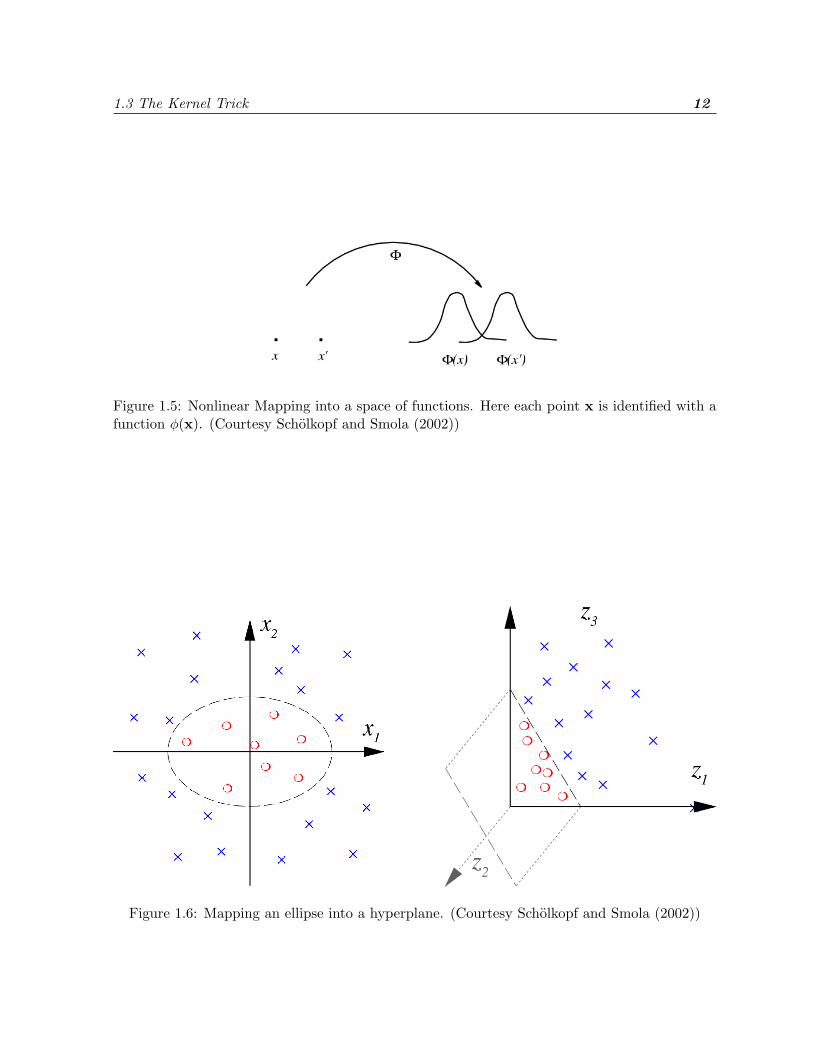
1.3 The Kernel Trick
In the previous section we assumed that the optimal decision surface was a linear hyperplane.
In real life situations this is a very restrictive assumption. But, suppose we can find a non-
linear mapping φ : Rd → Rk such that d � k and the data points are linearly separable in
Rk we can still use the linear SVM by replacing 〈xi,xj〉 with 〈φ(xi), φ(xj)〉 (cf. Figure 1.5).
Consider the toy example of a binary classification problem mapped into feature space shown
in Figure 1.6. We assume that the true decision boundary shown on the left is an ellipse in
input space. When mapped into feature space via the nonlinear map φ(x) = (z1, z2, z3) =
(|x1 |2, |x2 |2,√
2|x1 ||x2 |), the ellipse becomes a hyperplane, as shown on the right. It turns
out that certain class of functions which satisfy the Mercer’s conditions are admissible as kernels
1.3 The Kernel Trick 12
Figure 1.5: Nonlinear Mapping into a space of functions. Here each point x is identified with afunction φ(x). (Courtesy Scholkopf and Smola (2002))
Figure 1.6: Mapping an ellipse into a hyperplane. (Courtesy Scholkopf and Smola (2002))

1.3 The Kernel Trick 13
i.e. they can be written as
k(xi,xj) = 〈φ(xi), φ(xj)〉 ,
where φ is some non-linear mapping to a higher dimensional Hilbert space. Note that this
mapping is implicit, and, at no point do we actually need to calculate the mapping function
φ. As a result, all calculations are carried out in the space in which the data points reside. In
fact, a large class of algorithms which use similarity between points can be kernelized to work in
higher dimensional space. The rather technical Mercer’s condition is expressed as the following
two lemmas (Courant and Hilbert, 1953, 1962).
Lemma 4 If k is a continuous symmetric kernel of a positive integral operator K of the form
(Kf)(y) =∫
Ck(x,y)f(x) dx (1.13)
with ∫C×C
k(x,y)f(x)f(y) dx dy ≥ 0 (1.14)
for all f ∈ L2(C) where C is a compact subset of Rn, it can be expanded in a uniformly convergent
series (on C × C) in terms of eigenfunction ψj and positive eigenvalues λj
k(x,y) =NF∑j=1
λjψj(x)ψj(y), (1.15)
where NF ≤ ∞.
Lemma 5 If k is a continuous kernel of a positive integral operator, one can construct a map-
ping φ into a space where k acts as a dot product,
〈φ(x), φ(y)〉 = k(x,y). (1.16)
We refer the reader to (Scholkopf and Smola, 2002, Chapter 2) for an excellent technical discus-
sion on Mercer’s conditions and related topics.
In general, given data drawn from any domain X we can use SVM’s as long as we can find
a mapping φ : X → H, where H be any Hilbert space. Thus, the advantage of using SVM’s is
that we can work with non-vectorial data as long as the corresponding mapping to a Hilbert

1.4 Quadratic Soft-Margin Formulation 14
space can be found. In this thesis we exhibit many such mappings and give efficient algorithms
to compute them.
1.4 Quadratic Soft-Margin Formulation
In case we penalize the error points quadratically, the objective function Equation (1.6) is
modified as
minimizew,b
12‖w ‖2 + C
∑i
ξ2i
subject to yi (〈w,xi〉+ b) ≥ 1− ξi for all i ∈ {1, 2, . . . , n}.(1.17)
This formulation has been shown to be equivalent to the separable linear formulation in a space
that has more dimensions than the kernel space (Cortes and Vapnik, 1995, Freund and Schapire,
1999, Keerthi et al., 1999, Cristianini and Shawe-Taylor, 2000). In other words the quadratic loss
function gives rise to a modified hard-margin SV problem, where the kernel k(x, x′) is replaced
by k(x, x′) + χδx,x′ for some χ > 0. The above formulation where we penalize the error points
quadratically is also popularly known as the quadratic soft-margin loss or the `2 formulation. It
will be main focus of the SimpleSVM algorithm which we describe in Chapter 2.
1.5 Contributions and a Road Map of this Thesis
In Chapter 2 we present a fast iterative Support Vector training algorithm for the quadratic soft-
margin formulation. Our algorithm, which we christen the SimpleSVM, works by incrementally
changing a candidate Support Vector set using a locally greedy approach, until the supporting
hyperplane is found within a finite number of iterations. It is derived by a simple (yet computa-
tionally crucial) modification of the incremental SVM training algorithms of Cauwenberghs and
Poggio (2001) which allows us to perform update operations very efficiently. We also indicate
methods to extend our algorithm to the linear soft margin loss formulation.
The LDL> decomposition of a positive semi-definite matrix A ∈ Rn×n, where L ∈ Rn×n is
unit lower triangular and D ∈ Rn×n is diagonal, is popularly known as the Cholesky decompo-
sition. It is widely used in many applications because of its excellent numerical stability (Gill
et al., 1974). In general computing the LDL> decomposition of a n× n matrix requires O(n3)
computations while updating it after a rank one change in A requires O(n2) computations. In

1.5 Contributions and a Road Map of this Thesis 15
many applications of SVM’s, especially for the `2 formulation, the kernel matrix K ∈ Rn×n can
be written as K = ZZ> + Λ, where Z ∈ Rn×m with m� n and Λ is diagonal with nonnegative
entries. Hence the matrix K − Λ is rank-degenerate. In Chapter 3 we present an O(nm2) algo-
rithm to compute the LDL> factorization of such a matrix. We also show how rank-one updates
of such a factorization can be carried out in O(mn) time. We demonstrate the application of this
factorization to speed up the SimpleSVM algorithm. We also present applications to interior
point methods.
In Chapter 4 we try to provide a general overview of R-Convolution kernels proposed by
Haussler (1999). We produce many extensions and exhibit new kernels and also show how
various previous kernels can be viewed in this framework. This chapter provides general recipes
for defining kernels on strings, trees, Finite State Automata, images, etc. We also sketch a few
fast algorithms for computing kernels on sets. Specific implementation details and algorithms
for all other kernels are relegated to later chapters.
In Chapter 5 we present algorithms for computing kernels on strings (Watkins, 2000, Haus-
sler, 1999, Leslie et al., 2002a) and trees (Collins and Duffy, 2001) in linear time in the size of
the arguments, regardless of the weighting that is associated with any of the terms. We show
how suffix trees on strings can be used to enumerate all common substrings of two given strings.
This information can then be used to compute string kernels efficiently. In order to compute
kernels on trees we exhibit an algorithm to obtain the string representation of a tree. The string
kernel ideas are then used to compute kernels on trees. We discuss an algorithm for string
kernels by which the prediction cost can be reduced to linear cost in the length of the sequence
to be classified, regardless of the number of Support Vectors.
In Chapter 6 we explore the relationship between dynamical systems and kernels to define
kernels on dynamical systems with respect to a set of initial conditions and on initial conditions
with respect to an underlying dynamical system. This is achieved by comparing trajectories,
which leads to a large number of known and many novel kernels. We show, how, many previous
kernels can be viewed as special cases of our definitions and also propose many new kernels.
Using our definition we propose kernels on Markov Chains (discrete and continuous), diffusion
processes, graphs, linear time invariant systems, and Finite State Automata.
In Chapter 7 we describe a new method to generate virtual training samples in the case
of handwritten digit data. We use the two dimensional suffix tree representation of a set of

1.6 Summary 16
matrices to encode an exponential number of virtual samples in linear space, thus, leading to
an increase in classification accuracy. We propose a quadratic time algorithm for computing
kernels on images. Methods to reduce the prediction time to quadratic in the size of the test
image are also described.
We summarize the thesis in Chapter 8 with pointers for future research.
1.6 Summary
In this chapter we reviewed various ideas from machine learning and statistical learning theory.
We also showed why minimizing the empirical risk is not adequate for the classifier to generalize
and sketched the evolution of SVM’s from the ideas of statistical learning theory. We described
various optimization problems which arise out of different SVM formulations and discussed their
main features. We introduced the kernel trick and showed how it can help SVM’s handle non-
vectorial data. Finally, we presented the main contributions of this thesis in brief. The road
map will help the reader to locate chapters of specific interest.
Chapter 2
SimpleSVM: A SVM Training
Algorithm
This chapter is devoted to a detailed description of our Support Vector Machine (SVM) train-
ing algorithm called the SimpleSVM. SimpleSVM works mainly for the quadratic soft-margin
formulation (see Section 1.4 for details). It incrementally changes a candidate Support Vector
set using a locally greedy approach, until the supporting hyper plane is found within a finite
number of iterations.
We introduce our notation in Section 2.1 and also present some background. In Section 2.2
we discuss a few SVM training algorithms and show how the SimpleSVM is related to them.
We present a high level overview of our algorithm in Section 2.3. Detailed discussion of the
convergence properties follows in Section 2.4. We show finite time convergence and explain
why even exponential convergence is likely. Subsequently, in Section 2.5 we discuss the updates
required to change the Support Vector set in greater detail and present various initialization
strategies. Extensions of our method to the `1 formulation are sketched in Section 2.6. We
also briefly mention how SimpleSVM may benefit if the kernel matrix is rank-degenerate. This
extension is discussed in more detail in Chapter 3. Experimental evidence of the performance
of SimpleSVM is given in Section 2.7 and we compare it to other state-of-the art SVM training
algorithms. We conclude with a discussion in Section 2.8.
A few technical details concerning the factorization of matrices and their rank-one modifi-
cations is relegated to Appendix A. This is done, such that, only readers interested in imple-
menting the algorithm on their own will need to follow these derivations closely. Working code
17

2.1 Notation and Background 18
and datasets for our algorithm can be found at http://www.axiom.anu.edu.au/~vishy.
This chapter requires basic knowledge of SVM’s and the quadratic soft-margin formulation.
Readers may want to review these concepts from Chapter 1. For the convenience of readers
already familiar with these concepts and in order to make this chapter self contained the primal
and dual problems of the quadratic soft-margin formulation are repeated here. To understand
the dual formulation and its derivation some knowledge of optimization is helpful (but not
indispensable). A cursory knowledge of probability will help in understanding the constant time
initialization procedure.
2.1 Notation and Background
Training a SVM involves solving a quadratic optimization problem, which tends to be compu-
tationally intensive, is subject to stability problems and is non-trivial to implement. Attractive
iterative algorithms such as Sequential Minimal Optimization (SMO) by Platt (1999), the Near-
est Point Algorithm (NPA) by Keerthi et al. (2000), Lagrangian Support Vector Machines by
Mangasarian and Musicant (2001), Newton method using Kaufman-Bunch algorithm by Kauf-
man (1999) etc. have been proposed to overcome this problem. This chapter makes another
contribution in this direction.
In the following, we denote by {(x1, y1), . . . , (xn, yn)} ⊂ X ×{±1} the set of labeled training
samples, where xi are drawn from some domain X and yi ∈ {±1}, denotes the class labels +1 and
−1 respectively. Furthermore, let n be the total number of points and let n+ and n− denote the
number of points in class +1 and −1 respectively. With some abuse of notation we will associate
with each set A ⊆ {1, . . . , n} the corresponding set of observations S(A) := {(xi, yi)|i ∈ A} and
denote by |A| the cardinality of A, with m := |A| being the (current) number of support vectors.
Denote by k : X ×X → R, a Mercer kernel and by Φ : X → F , the corresponding feature
map, that is 〈Φ(x),Φ(x′)〉 = k(x,x′) (see Section 1.3 for more details). In this chapter we study
the quadratic soft-margin loss function discussed in Section 1.4. Consequently, in the following,
we assume that we are dealing with a hard-margin SVM where a separating hyperplane can be
found, possibly with k(x,x′)← k(x,x′) + χδx,x′ .

2.2 Related Work 19
2.2 Related Work
DirectSVM: It has been shown that the closest pair of points of the opposite class are SV’s.
Hence, DirectSVM (Roobaert, 2000) starts off with this pair of points in the candidate
SV set. It works on the conjecture that the point which incurs the maximum error (i.e.,
minimal yif(xi)) during each iteration is a SV. This violating point is found and added to
the SV set.
In case the dimension of the space is exceeded or all the data points are used up, without
convergence, the algorithm reinitializes with the next closest pair of points from opposite
classes (Roobaert, 2000). The problem with DirectSVM is that its approach to adding a
new point to the SV set is very costly.
GeometricSVM: Vishwanathan and Murty (2002a) proposed an optimization based approach
to add new points to the candidate SV thus improving the scaling behavior of DirectSVM.
Unfortunately, neither DirectSVM nor GeometricSVM has a provision to backtrack, i.e.
once they decide to include a point in the candidate SV set they cannot discard it. During
each iteration, both the algorithms spend their maximum effort in finding the maximum
violator. Caching schemes can be used to alleviate this problem, but, they require a large
cache size for large datasets, besides, the scaling behavior of such caching schemes is not
well understood (Vishwanathan and Murty, 2002a).
Newton Approach: Kaufman (1999) proposed a Newton approach based on the Bunch-Kaufman
algorithm. It maintains a s × s matrix of active constraints which is updated in O(s2)
time when a constraint is added or deleted. It finds the first constraint to be violated by
finding the gradient of the function and hence computing the change in all the constraints.
The main drawback of this method is that computing the gradient is a costly operation
and the algorithm has to compute the gradient for every iteration. Both, SimpleSVM and
the Kaufman (1999) algorithm maintain an active set and update it during each iteration.
This idea is studied under the name of inertia controlling methods for general Quadratic
Programs (QP). We refer the reader to Gill et al. (1991) for a survey of such techniques.
Incremental and Decremental SVM: Cauwenberghs and Poggio (2001) proposed an incre-
mental SVM algorithm, where, at each step only one point is added to the training set. If

2.3 The Basic Idea 20
the added point violates the KKT conditions one recomputes the exact SV solution of the
whole dataset seen so far.
After the addition of each point, the algorithm maintains the exact solution for the whole
dataset seen so far. Hence, after n points have been added, the algorithm finds the exact
solution for the entire training set, and thus converges in n steps (Cauwenberghs and
Poggio, 2001). Unfortunately, the condition to remain optimal at every step means that,
whenver a violating point is found, the algorithm has to test all the observations seen so
far. Such a requirement dramatically slows it down.
In particular, it means that the algorithm has to perform n′|A| kernel computations at
each step, where n′ denotes the number of observations seen so far and A is the current SV
set. This is clearly expensive. Cauwenberghs and Poggio (2001) suggest a practical on-line
variant where they introduce a δ margin and concentrate only on those points which are
within the δ margin of the boundary. But, it is clear that the results may vary by varying
the value of δ.
The way to overcome the limitations of the Cauwenberghs and Poggio (2001) and Kaufman
(1999) algorithms is to require that the new solution strictly decrease the margin of separation
and be optimal with respect to a subset of A ∪ {v}, where (xv, yv) satisfies yvf(xv) < 1. This
is a greedy approach which does not guarantee that we are making optimal progress towards
the final solution, instead, we perform a small amount of work and strictly decrease the margin
of separation to obtain the final solution after a finite number of steps. In this sense one could
interpret SimpleSVM as being related to the Incremental and Decremental SVM and the Newton
method.
2.3 The Basic Idea
In spirit, our algorithm is very much related to the chunking methods developed at AT&T
Bell Laboratories (Burges and Vapnik, 1995). There, SV training is carried out by splitting an
overly large training set into small chunks, train on the first one, keep the SV’s, add the next
chunk, retrain, keep the SV’s, etc. until all the points satisfy the Karush-Kuhn-Tucker (KKT)
conditions (see also Cortes (1995)).

2.3 The Basic Idea 21
Algorithm 2.1: SimpleSVMinput Dataset Z
Initialize: Find any sufficiently close pair from opposing classes (xi+ , xi−)A← {i+, i−}Compute f and α for Awhile there are xv with yvf(xv) < 1 doA← A ∪ {v}Recompute f and α and remove non-SV’s from A.
end whileOutput: A, {αi for i ∈ A}
Osuna et al. (1997), Joachims (1999) and Platt (1999) generalize this strategy by dropping
the requirement of optimality on all the points with nonzero αi. Instead, they fix some variables
while optimizing over the remainder, regardless of their value of αi. In particular, SMO optimizes
only over two observations at a time and computes the minimum in closed form. This strategy
has proven successful whenever the number of nonzero coefficients αi is large, that is, the dataset
is noisy, and the hypothesis-to-be-found is not too complex (Scholkopf and Smola, 2002).
The AT&T Bell Laboratories style optimization method, however, also admits another mod-
ification: add only one point to the set of SV’s at a time and compute the exact solution. If
we had to recompute the solution from scratch this would be an extremely wasteful procedure.
Instead, as we will see in Section 2.4, it is possible to perform such computations at O(m2)
cost, where m is the number of current SV’s and obtain the exact solution on the new subset of
points. Even better, if the kernel matrix is rank-degenerate of rank d, updates can be performed
at O(md) cost using a novel factorization method of Smola and Vishwanathan (2003), thereby
further reducing the computational burden (see Chapter 3 for more details on our factoriza-
tion). As one would expect, this modification will work well whenever the number of SV’s is
small relatively to the size of the dataset, that is, for “clean” datasets.
While there is no guarantee that one sweep through the data set will lead to a full solution of
the optimization problem (and it almost never will, since some points may be left out which will
become SV’s at a later stage), we empirically observed that a small number of passes through
the entire dataset (typically less than 4) is sufficient for the algorithm to converge. Algorithm 2.1
gives a high-level description of the simple steps involved in SimpleSVM.
2.4 SimpleSVM 22
2.4 SimpleSVM
In this section we show that SimpleSVM finds the hard-margin solution and we analyze its
properties. We begin by studying the optimization problem dual to finding the maximum
margin. Next we show that adding a new point to A will always decrease the dual objective
function and we will use this fact to show finite time convergence. Finally, we indicate why one
may obtain linear convergence based on coordinate descent argument.
2.4.1 The Dual Problem
In the case of hard-margin SVM the set of current Support Vectors A is also the set of active
constraints (hence, in the following, we will refer to A interchangeably). It is well known that
the dual problem to the maximum margin problem
minimizew,b
12‖w ‖
2
subject to yi (〈w,Φ(xi)〉+ b) ≥ 1 for all i ∈ A(2.1)
is given by
maximizeα
−12α>Hα+
∑i
αi
subject to∑
i
αiyi = 0 and αi ≥ 0 for all i ∈ A and αi = 0 for all i 6∈ A(2.2)
Here H ∈ Rn×n with Hij := yiyjk(xi, xj). Moreover, it is a basic fact from optimization theory
(Mangasarian, 1969) that the minimum of Equation (2.1) equals the maximum of Equation (2.2).
Furthermore, Boser et al. (1992) showed that the value of Equation (2.1) is given by 12ρ2 , where
ρ is the margin between the two classes with respect to the subsets chosen via A.
2.4.2 Finite Time Convergence
By construction, adding elements to A, can only increase the value of Equation (2.1) (or leave
it constant), since we are shrinking the feasible set. In other words, adding a violating point can
only decrease the margin of separation. Moreover, dropping elements from A which correspond
to strictly satisfied constraints will not change the value of the optimization problem. Finally,
since by assumption the solution of Equation (2.1) exists, adding elements to A which correspond
2.4 SimpleSVM 23
to strictly violated constraints in Equation (2.1) is guaranteed to increase the value of the primal
objective function. We therefore have the following lemma:
Lemma 6 (Strictly Improving Updates) At every step, where SimpleSVM adds some {v}
with yvf(xv) < 1 to A, the optimal margin of separation with respect to A must decrease.
Furthermore, dropping the non-SV’s from A will not change the margin.
Now we can show finite time convergence. Key to the proof is the fact that there exists only a
finite number of sets A.
Theorem 7 (Convergence of SimpleSVM) SimpleSVM converges to the hard-margin solu-
tion in a finite number of steps.
A relaxed version of the algorithm, which only finds solutions on A ∪ {v}, that are optimal
with respect to A′ ⊆ A∪{v} also will converge in a finite number of steps, as long as the objective
function in A′ is strictly larger than the one in A.
Proof Let A be the candidate SV set at the end of an iteration (i.e. after a violating point has
been added and all those points with negative α’s have been discarded.) The KKT conditions
of Equation (2.2) are both necessary and sufficient conditions for optimality. Since, the solution
found by SimpleSVM satisfies the KKT conditions it is an optimal solution of Equation (2.1)
with respect to the current A. Furthermore, SimpleSVM terminates only if A contains all active
constraints in Equation (2.1) from {1, . . . , n}. This, however, is the hard-margin solution.
On the other hand, by virtue of Lemma 6, as long as SimpleSVM performs updates, the value
of Equation (2.1) with respect to the current A is strictly increasing. Thus, the algorithm cannot
cycle back to the same A. However, there exist only a finite number of sets A ⊆ {1, . . . , n}, hence
the series of values of Equation (2.1) corresponding to the current A must converge to some value
in a finite number of steps. By the above reasoning, this must be the optimal solution.
The same reasoning holds for the relaxed version which only finds solutions optimal in
A′ ⊆ A ∪ {v}, as long as the objective function is strictly increasing.
2.4.3 Rate of Convergence
By Theorem 7 we know that Algorithm 2.1 does not cycle and instead it will visit every variable
(of which we have only finitely many) at a time. To show linear convergence, note that we are

2.5 Updates 24
performing updates which are strictly better than coordinate descent at every step (in coordinate
descent we only optimize over one variable at a time, whereas in our case we optimize over
A ∪ {v} which includes a new variable at every step). Coordinate descent, however, has linear
convergence for strictly convex functions Fletcher (1989).
2.5 Updates
This section contains the central details of the updates required for adding and removing points,
plus strategies for initializing the algorithm. Here we show how updates can be performed
cheaply without the need for many kernel computations.
2.5.1 Initialization
Since we want to find the optimal separating hyperplane of the overall dataset Z, a good starting
point is the pair of observations (x+, x−) from opposing sets X+, X− closest to each other
(Roobaert, 2000). Brute force search for this pair costs O(n2) kernel evaluations, which is
clearly not acceptable for the search of a good starting point. The algorithms by Bentley and
Shamos (1976) and Vaidya (1989) find the find best pair in log linear time for multi-dimensional
data points.
Another approach is to use approximate closest pair of points. Since, our algorithm does
not critically depend on the pair of points chosen for initialization, this approach is acceptable.
Denote by ξ := d(x+, x−) the random variable obtained by randomly choosing x+ ∈ X+ and
x− ∈ X−. Then the shortest distance between a pair x+, x− is given by the minimum of the
random variables ξ. Therefore, if we are only interested in finding a pair whose distance is, with
high probability, much better than the distance of any other pair, we need only draw random
pairs and pick the closest one.
In particular, one can check (Scholkopf and Smola, 2002) that roughly 59 pairs are sufficient
for a pair better than 95% of all pairs with 0.95 probability, and to be better than 99.9% of all
pairs with 0.999 probability we need to draw from only 7000 pairs (in general, we need log δlog(1−δ) ≈
δ−1 log δ observations to be better than a fraction of 1− δ samples with 1− δ probability). For
other fast algorithms for approximate closest pair queries see Gionis et al. (1999), Indyk and
Motawani (1998).

2.5 Updates 25
Once a good pair (x+, x−) has been found, we need to initialize the corresponding α+, α−
and b. This is done by solving the linear system of equations:
f(x+) + b = K++α+ −K+−α− + b = 1
−f(x−)− b = −K−+α+ +K−−α− − b = 1
α+ − α− = 0
(2.3)
This operation can be carried out in constant time.
2.5.2 Adding a Point
Now we proceed to the updates necessary for adding an observation to the set of SV’s. The
cheapest strategy is to progress linearly through the dataset. Other strategies to locate violating
points have the disadvantage of requiring a larger number of computations. For every new
observation (xv, yv) with v 6∈ A, two cases may occur:
yvf(xv) ≥ 1: This point is currently correctly classified, so we need not perform any updates.
We retain A and proceed to the next point.
yvf(xv) < 1: This point will become a Support Vector, since at present it is wrongly classi-
fied. By default we assume that A← A ∪ {v} (we deal with pruning other points in Sec-
tion 2.5.3) and that therefore all xi with i ∈ A must satisfy yif(xi) = 1 and∑
i∈A αiyi = 0.
In matrix notation this reads as follows: 0 y>A
yA HA
b
αA
=
0
e
. (2.4)
Here yA ∈ {−1, 1}|A| is the vector of yi corresponding to A, αA ∈ R|A|, HA ∈ R|A|×|A|
satisfies (HA)ij = yiyjk(xi, xj), and e ∈ R|A| is the vector of ones.
Consequently, adding one element to A means that we have to solve the linear system
Equation (2.4), which has been increased by one row and column, given the solution of
the smaller system.
Such rank-one modifications of linear systems are standard in numerical analysis and are
discussed in great detail in Golub and Loan (1996), Horn and Johnson (1985). In a nutshell,

2.5 Updates 26
the operation can be carried out in O(|A|2) time. The adaptation to the current problem
is described in Appendix A.
2.5.3 Removing a Point
In case the linear system Equation (2.4) leads to a solution containing negative values of αv on
the set A ∪ {v} we need to remove elements from A ∪ {v}, since points in A ∪ {v} have ceased
to be support vectors.
We will use an efficient variant of the “adiabatic increments” strategy from Cauwenberghs
and Poggio (2001) for our purposes. Two problems arise: which points to remove (and in which
order) to obtain a linear system for which all αi are nonnegative, and how to avoid having to
check all removed points whether they might become SV’s again (unlike in incremental SVM
learning, where such checks may contribute a significant amount of computation to the overall
cost of an update). In a nutshell, the strategy will be to remove one point at a time while
maintaining a strictly dual feasible set of variables.
We need a few auxiliary results. For the purpose of the proofs we assume that all xi with
i ∈ A ∪ {v} are linearly independent. The general proof strategy works as follows: first we show
that the infeasible set of variables arising from changing A into A ∪ {v} is the solution of a
modified optimization problem. Subsequently, we prove that adiabatic changes strictly increase
the value of ‖w‖2 while reducing the number of active constraints and rendering the resulting
solution less infeasible.
Lemma 8 (Changed Margin) Assume we have a set of coefficients αi ≥ 0 with i ∈ A ∪ {v}
and b ∈ R with∑
i∈A∪{v} yiαi = 0 and w :=∑
i∈A∪{v} αiyixi, such that yi(〈w, xi〉+b) = 1 for all
i ∈ A and yv(〈w, xv〉+ b) = ρ. Then (w, b) is the solution of the following optimization problem:
minimize 12‖w‖
2
subject to yi(〈w, xi〉+ b) ≥ 1 for all i ∈ A and yv(〈w, xv〉+ b) ≥ ρ.(2.5)
Proof The optimization problem Equation (2.5) is almost identical to the SVM hard-margin
classification problem, except for one modified constraint on (xv, yv). It is easy to check that the
dual optimization problem to Equation (2.5) has identical dual constraints to the SVM hard-
margin problem (only in the objective function the linear contribution of αv is changed from
1 · αv to ρ · αv).

2.5 Updates 27
By construction (w, b) is a feasible solution of Equation (2.5), the set of αi is dual feasible
and finally, by construction, the KKT conditions are all satisfied. From duality theory it fol-
lows (see e.g., Vanderbei (1997)) that such a set of variables constitutes an optimal solution of
Equation (2.5), which proves the claim.
Lemma 9 (Shifting) In addition to the assumptions of Lemma 8 denote by (α′, b′) with w′ :=∑i∈A∪{v} α
′iyixi the solution of the linear system
1 = yi(〈w, xi〉+ b) for all i ∈ A ∪ {v} and 0 =∑
i∈A∪{v}
yiαi. (2.6)
Then (α, b) = (1− λ)(α, b) + λ(α′, b′) with w = (1− λ)w+ λw′ is a solution of the optimization
problem Equation (2.5) with corresponding ρ = (1 − λ)ρ + λ, as long as all αi ≥ 0 for all
i ∈ A ∪ {v}.
Proof We first show that α and b satisfy the conditions of Lemma 8. By construction, α′ is
nonnegative, it satisfies the summation constraint∑
i∈A∪{v} yiαi, since it is a convex combina-
tion of α and α′, which both satisfy the constraint. Moreover, yi(〈w, xi〉 + b) = 1 for all i ∈ A
(again, since this holds for both (α, b) and (α′, b′)). Finally, the value of b also can be found as
a convex combination of ρ and ρ′ = 1.
Lemma 10 (Piecewise Optimization) We use the assumptions in Lemma 8 and 9 for (α, b, w),
(α′, b′, w′), (α, b, w). In addition to that we assume that αi > 0 for all i ∈ A and ρ < 1. Then
for λ given by
λ := min(
1, mini|α′i<0
(αi
αi − α′i
))(2.7)
we have ‖w‖2 < ‖w′‖2 and ρ < ρ′ ≤ 1. Moreover, if λ < 1 we have αi = 0 for some i ∈ A.
Proof By construction, λ > 0, since αj > 0 for all j ∈ A and α′j is finite (the xj are linearly
independent). From Lemma 9 we know that ρ = (1− λ)ρ+ λ > (1− λ)ρ+ λρ = ρ. Since (α, b)
is a solution of an optimization problem with a further restricted domain, obtained by replacing
ρ with ρ. Since the constraints were active for ρ, this implies that ‖w‖2 must increase as we

2.6 Extensions 28
Algorithm 2.2: Removing Points from A ∪ {v}Input: A ∪ {v}, α, brepeat
Compute α′, b′ by solving Equation (2.6)Compute λ according to Equation (2.7)Update α← (1− λ)α+ λα′ and b← (1− λ)b+ λb′.if λ < 1 then
Remove from A for which λ was attained.Update matrices and intermediate values needed for computing new α′, b′.
end ifuntil λ = 1Output: A, α, b
restrict the domain. The conclusion that some αj = 0 follows directly from the choice of λ: the
coefficient vanishes for the argmin of Equation (2.7).
Putting everything together we have an algorithm to perform the removals from A ∪ {v} while
being guaranteed to obtain larger ‖w‖2 as we go (Algorithm 2.2). At every step the value of
‖w‖2 must increase, due to Lemma 10. Furthermore, at the end of the optimization process,
we will have a solution (α, b) which is a SVM solution with respect to the new set A ∪ {v}
(where A possibly was shrunk). This ensures that we make progress at every step of the main
SimpleSVM algorithm (even though the new solution may not be optimal with respect to the
original A ∪ {v}).
Technical details on how α′, b′ are best computed and how the corresponding matrices can
be updated are relegated Appendix A. It is worth while noting that each of the steps in
Algorithm 2.2 comes at the cost of O(|A|2) operations, which may seem rather high. However,
note that whenever we remove a point from A, all further increments will incur a smaller cost,
so removing as many elements from A as possible is highly desirable.
2.6 Extensions
2.6.1 Rank-Degenerate Kernels
Regardless of the type of matrix factorization we use to compute the SV solutions on A, we will
still encounter the problem that the memory requirements scale with O(|A|2) and the overall
computation is of the order of O(|A|3 + |A|n) for the whole algorithm. This may be much better
2.6 Extensions 29
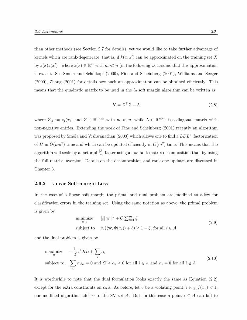
than other methods (see Section 2.7 for details), yet we would like to take further advantage of
kernels which are rank-degenerate, that is, if k(x, x′) can be approximated on the training set X
by z(x)z(x′)> where z(x) ∈ Rm with m� n (in the following we assume that this approximation
is exact). See Smola and Scholkopf (2000), Fine and Scheinberg (2001), Williams and Seeger
(2000), Zhang (2001) for details how such an approximation can be obtained efficiently. This
means that the quadratic matrix to be used in the `2 soft margin algorithm can be written as
K = Z>Z + Λ (2.8)
where Zij := zj(xi) and Z ∈ Rn×m with m � n, while Λ ∈ Rn×n is a diagonal matrix with
non-negative entries. Extending the work of Fine and Scheinberg (2001) recently an algorithm
was proposed by Smola and Vishwanathan (2003) which allows one to find a LDL> factorization
of H in O(nm2) time and which can be updated efficiently in O(m2) time. This means that the
algorithm will scale by a factor of |A|m faster using a low-rank matrix decomposition than by using
the full matrix inversion. Details on the decomposition and rank-one updates are discussed in
Chapter 3.
2.6.2 Linear Soft-margin Loss
In the case of a linear soft margin the primal and dual problem are modified to allow for
classification errors in the training set. Using the same notation as above, the primal problem
is given by
minimizew,b
12‖w ‖
2 + C∑m
i=1 ξi
subject to yi (〈w,Φ(xi)〉+ b) ≥ 1− ξi for all i ∈ A(2.9)
and the dual problem is given by
maximizeα
−12α>Hα+
∑i
αi
subject to∑
i
αiyi = 0 and C ≥ αi ≥ 0 for all i ∈ A and αi = 0 for all i 6∈ A(2.10)
It is worthwhile to note that the dual formulation looks exactly the same as Equation (2.2)
except for the extra constraints on αi’s. As before, let v be a violating point, i.e. yvf(xv) < 1,
our modified algorithm adds v to the SV set A. But, in this case a point i ∈ A can fail to

2.7 Experiments 30
become a Support Vector either because αi < 0 or αi > C. We check for both these conditions
and remove such non-Support Vectors from A. While removing these non-Support Vectors, if
αv > C, we drop v and proceed to the next violating point. Proof of convergence of this modified
algorithm and its performance on real life datasets is a topic of current research.
2.7 Experiments
Since the main goal of this chapter is to give an algorithmic improvement over existing SVM
training algorithms, we will not report generalization performance figures here (they are irrele-
vant for properly converging algorithms, since all of them minimize the same objective function).
Instead, we will compare our method with the performance of the NPA algorithm by Keerthi
et al. (2000). NPA was chosen, since its authors showed in their experiments that it is compet-
itive with or better than other methods (such as SVMLight or SMO).
In particular, we will be comparing the number of kernel evaluations performed by a Support
Vector algorithm as an effective measure of its speed. Other measures are fraught with difficulty,
since comparing different implementations, compilers, platforms, operating systems, etc., causes
a large amount of variation even between identical algorithms.
2.7.1 Experimental Setup and Datasets
All experiments were run on a 800 MHz, Intel Pentium III machine with 128MB RAM running
Linux Mandrake 8.0 (unless mentioned otherwise). The code was written in C++ as well as in
MATLAB1. We use the full kernel matrix for all our experiments.
We uniformly used a value of 0.001 for the error bound i.e. we stop the algorithm when
yif(xi) > 0.999 ∀i. The NPA results are those reported in Keerthi et al. (1999). Consequently
we used the same kernel, namely a Gaussian RBF kernel with
k(x, x′) = exp(− 1
2σ2‖x− x′‖2
). (2.11)
The datasets chosen for our experiments are described in Table 2.1. The Spiral dataset was
proposed by Alexis Wieland of MITRE Corporation and it is available from the CMU Artificial
Intelligence repository. Both WPBC and the Adult datasets are available from the UCI Machine
1Code and datasets are available under the GPL at http://axiom.anu.edu.au/~vishy

2.7 Experiments 31
Table 2.1: Datasets used for the comparison of SimpleSVM and NPADataset Size Dimensions σ2
Spiral 195 2 0.5WPBC 683 9 4Adult-1 1,605 123 10Adult-4 4,781 123 10Adult-7 16,100 123 10
Learning repository (Blake and Merz, 1998). We used the same values of σ2 as in Keerthi et al.
(1999) and Platt (1999) to allow for a fair comparison. Experimental results can be found in
Figures 2.1 to 2.10.
Figure 2.1: Performance comparison between SimpleSVM and NPA on the Spiral dataset.
2.7.2 Discussion of the Results
As can be seen SimpleSVM outperforms the NPA considerably on all five datasets. For instance,
on the Spiral dataset the SimpleSVM is an order of magnitude faster than the NPA. On the
Adult-4 dataset with C = 1000 the SimpleSVM algorithm is nearly 50 times faster than the
NPA.
Furthermore, unlike NPA, SimpleSVM’s runtime behavior, given by the number of kernel

2.7 Experiments 32
Figure 2.2: Total number of times a point was ever added to the initial Support Vector setcompared with the final number of Support Vectors on the Spiral dataset.
Figure 2.3: Performance comparison between SimpleSVM and NPA on the WPBC dataset.

2.7 Experiments 33
Figure 2.4: Total number of times a point was ever added to the initial Support Vector setcompared with the final number of Support Vectors on the WPBC dataset.
Figure 2.5: Performance comparison between SimpleSVM and NPA on the Adult-1 dataset.

2.7 Experiments 34
Figure 2.6: Total number of times a point was ever added to the initial Support Vector setcompared with the final number of Support Vectors on the Adult-1 dataset.
Figure 2.7: Performance comparison between SimpleSVM and NPA on the Adult-4 dataset.

2.7 Experiments 35
Figure 2.8: Total number of times a point was ever added to the initial Support Vector setcompared with the final number of Support Vectors on the Adult-4 dataset.
Figure 2.9: Performance comparison between SimpleSVM and NPA on the Adult-7 dataset.

2.7 Experiments 36
Figure 2.10: Total number of times a point was ever added to the initial Support Vector setcompared with the final number of Support Vectors on the Adult-7 dataset.
evaluations, does not critically depend on the value of χ (see for instance Figures 2.1 and 2.5).
The ratio between the total number of points ever added to the initial Support Vector set
(initially the set contains two points) and the final number of Support Vectors indicates the
number of times a “wrong” Support Vector is picked or a point is recycled. As can be seen the
penalty incurred due to our greedy approach is not very significant (see for instance Figures 2.2
and 2.4).
Also note that, by construction SimpleSVM computes an exact solution on its SV set, whereas
algorithms such as NPA will only yield approximate expansions. In all but one case (in the Adult-
7 dataset) the number of Support Vectors found by our algorithm and the NPA differs by at
most 2. One possible explanation for the difference on the Adult-7 data is that the stopping
criterion employed by the two algorithms are different. Round off errors due to differences in
the precisions used for the computations may further aggravate the problem.
2.8 Summary and Outlook 37
2.8 Summary and Outlook
We presented a new SV training algorithm that is efficient, intuitive, and fast. It significantly
outperforms other iterative algorithms like the NPA in terms of the number of kernel computa-
tions. Moreover, it does away with the problem of overall optimality on all previously seen data
that was one of the major drawbacks of Incremental SVM, as proposed by Cauwenberghs and
Poggio (2001). But, the cost incurred due to this relaxation is that our algorithm is no longer
an incremental algorithm.
It should be noted that SimpleSVM performs particularly well whenever the datasets are
relatively “clean”, that is, whenever the number of SV’s is rather small. On noisy data, on the
other hand, methods such as SMO may be preferable to our algorithm. This is mainly due to
the fact that a matrix of size of the kernel matrix needs to be stored in memory (256 MB of main
memory suffice to store a matrix corresponding to as many as 10, 000 SV’s). Storage therefore
becomes a serious limitation of SimpleSVM when applied to generic dense matrices on large noisy
datasets. One possibility to address this problem is to use low-rank approximation methods
which make the problem amenable to the low-rank factorizations described in Section 2.6.1.
Due to the LDL> factorization used in finding the SV solution our algorithm is numerically
more stable than using a direct matrix inverse. This helps us deal with round off errors that can
plague other algorithms. We suspect that similar modifications could be successfully applied to
other algorithms as well.
Our algorithm can be sped up further by the use of a kernel cache. The effect of the use of
cache is an area of further study. Based on this study an efficient kernel cache can be designed
for our algorithm.
It can be observed that the addition of a vector to the Support Vector set is entirely reversible.
Using this property and following the derivation in Opper and Winther (2000), Cauwenberghs
and Poggio (2001) calculated the leave one out error. Similar techniques could be used in the
context of SimpleSVM, too.

Chapter 3
Modified Cholesky Factorization
This chapter presents an algorithm to compute the Cholesky decomposition of a special class
of matrices which occur frequently in machine learning and Support Vector Machine (SVM)
training. In many applications of SVM’s, especially for the `2 formulation, the kernel matrix
K ∈ Rn×n is can be written as K = ZZ>+Λ, where Z ∈ Rn×m with m� n and Λ is a diagonal
matrix with non-negative entries. Hence the matrix K − Λ is rank-degenerate. This chapter
presents an O(nm2) algorithm to compute the LDL> factorization of such a matrix. An O(mn)
algorithm to carry out rank-one updates of such a factorization is also discussed. Application of
the factorization to speed up the SimpleSVM algorithm and interior point methods is described.
Section 3.2 contains the main result, namely an LDL> factorization algorithm for matrices
of type ZZ> + Λ. We present implementation details along with methods for parallelizing such
a factorization. In Section 3.3 we show how a modified version of our factorization can be used
to obtain an (implicit) LDV decomposition of Z at O(m3) cost. Subsequently, in Section 3.4
we study how rank-1 modifications and row/column removal can be dealt with most efficiently
when an initial factorization has already been obtained. Two applications are presented in
Section 3.5: interior point optimization and a Support Vector classification algorithm. Lazy
methods to reduce the computational burden are also discussed. We conclude the chapter with
a discussion in Section 3.6.
This chapter requires the reader to thoroughly understand the concept of the Cholesky
decomposition of a positive semi-definite matrix. See Stewart (2000) for a survey of matrix
factorization. Understanding of concepts from linear algebra is required to appreciate the proofs
of theorems in this chapter. We highly recommend the book by Strang (1998). Knowledge of the
38

3.1 Introduction 39
SimpleSVM algorithm is essential to appreciate the material discussed in Section 3.5. Readers
may want to read Chapter 2 which discusses the SimpleSVM algorithm in detail before reading
this chapter. Familiarity with interior point methods and parallel algorithms is also assumed at
many places in the chapter.
3.1 Introduction
Consider the system of equations
Ax = b (3.1)
where A ∈ Rn×n and b ∈ Rn. It is well known that x should be computed by some factorization
of A rather than by a direct computation of A−1 (Golub and Loan, 1996). If A is positive
semi-definite, it can be factored as A = LDL>, where L is a unit lower triangular matrix and
D is a diagonal matrix containing only non-negative entries. Standard methods for finding such
factorizations exist and require at least O(n3) operations (see Golub and Loan (1996), Horn and
Johnson (1985), Stoer and Bulirsch (1993) for references and details).
In many applications including Support Vector Machines (SVM) and interior point methods,
the matrix A can be written as
A = ZZ> + Λ, (3.2)
where Z ∈ Rn×m with m � n and Λ is a diagonal matrix with non-negative entries. In this
chapter we present an algorithm to compute the LDL> factorization of such a matrix in O(nm2)
time. We also show how our factorization can be used to solve Equation (3.1) in O(mn) time.
3.1.1 Previous Work
Conventional wisdom to solve Equation (3.1) for the special case of Equation (3.2) is to perform
m rank-1 updates of an LDL> factorization and use this product factorization, that is
A = LmLm−1 . . . L1DL>1 . . . L
>m−1L
>m. (3.3)
Here all Li are special lower triangular matrices. Such methods were suggested e.g., in Gill et al.
(1974), Goldfarb and Scheinberg (2001), Fine and Scheinberg (2001).
While a factorization of type Equation (3.3) is efficient in the sense that it exhibits the right

3.1 Introduction 40
scaling behavior of O(m2n) operations to factorize and O(mn) operations to solve the linear
system, it has several downsides:
• It is difficult to perform rank-1 modifications on A once its factorization has been com-
puted. Such operations occur frequently when solving families of optimization problems
which differ only slightly in the number of constraints.
• Operations needed for iterative factorizations, and especially the solution of the overall
system, cannot be easily vectorized.
• A factorization in terms of products of terms L1, . . . , Lm cannot easily be parallelized.
Our proposed factorization method, which we will describe in Section 3.2 addresses all three
issues. We give a detailed account on some applications of the new factorization in Section 3.5.
An alternative approach to solving the problem is to use the Sherman-Morrison-Woodbury
(SMW) formula (Golub and Loan, 1996) via
y =[Λ−1 − Λ−1Z(Z>ΛZ + 1m)−1ZΛ−1
]x . (3.4)
While it has been used successfully in some convex optimization problems (Ferris and Munson,
2000), such methods tend to be numerically less stable, in particular if Λ is ill conditioned, as
pointed out by Fine and Scheinberg (2001).
3.1.2 Notation
We denote matrices by capital letters, e.g., Z ∈ Rn×m, vectors by boldface characters, e.g.,
z ∈ Rm, and scalars by lowercase characters, e.g., z ∈ R. Let 1n be the unit matrix in Rn×n,
and 0 be the vector with appropriate number of zero entries. We denote by Zij the entries of
Z and, unless stated otherwise, zi will denote the ith column of Z> and zi the ith entry of z.
Also, unless stated otherwise, we assume vectors to be column-vectors, i.e., we assume that z> z
is a scalar. Moreover, i, j, k,m, n ∈ N are integers and throughout the chapter m ≤ n. The
matrices D and Λ are diagonal matrices and we will address their diagonal entries as Di and Λi
respectively. ‖A‖ denotes the 2-norm of A, considered as linear mapping.
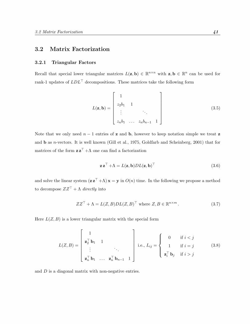
3.2 Matrix Factorization 41
3.2 Matrix Factorization
3.2.1 Triangular Factors
Recall that special lower triangular matrices L(z,b) ∈ Rn×n with z,b ∈ Rn can be used for
rank-1 updates of LDL> decompositions. These matrices take the following form
L(z,b) =
1
z2b1 1...
. . .
znb1 . . . znbn−1 1
(3.5)
Note that we only need n − 1 entries of z and b, however to keep notation simple we treat z
and b as n-vectors. It is well known (Gill et al., 1975, Goldfarb and Scheinberg, 2001) that for
matrices of the form z z> +Λ one can find a factorization
z z> +Λ = L(z,b)DL(z,b)> (3.6)
and solve the linear system (z z> +Λ)x = y in O(n) time. In the following we propose a method
to decompose ZZ> + Λ directly into
ZZ> + Λ = L(Z,B)DL(Z,B)> where Z,B ∈ Rn×m . (3.7)
Here L(Z,B) is a lower triangular matrix with the special form
L(Z,B) =
1
z>2 b1 1...
. . .
z>n b1 . . . z>n bn−1 1
i.e., Lij =
0 if i < j
1 if i = j
z>i bj if i > j
(3.8)
and D is a diagonal matrix with non-negative entries.
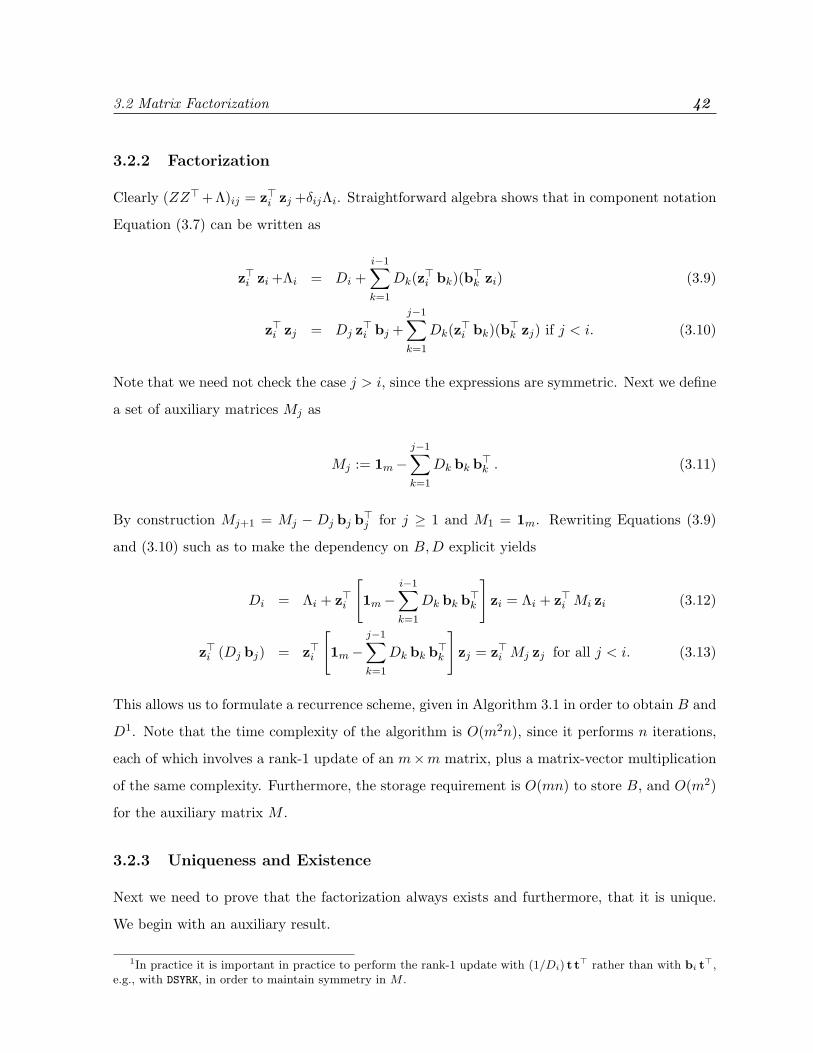
3.2 Matrix Factorization 42
3.2.2 Factorization
Clearly (ZZ>+Λ)ij = z>i zj +δijΛi. Straightforward algebra shows that in component notation
Equation (3.7) can be written as
z>i zi +Λi = Di +i−1∑k=1
Dk(z>i bk)(b>k zi) (3.9)
z>i zj = Dj z>i bj +j−1∑k=1
Dk(z>i bk)(b>k zj) if j < i. (3.10)
Note that we need not check the case j > i, since the expressions are symmetric. Next we define
a set of auxiliary matrices Mj as
Mj := 1m−j−1∑k=1
Dk bk b>k . (3.11)
By construction Mj+1 = Mj − Dj bj b>j for j ≥ 1 and M1 = 1m. Rewriting Equations (3.9)
and (3.10) such as to make the dependency on B,D explicit yields
Di = Λi + z>i
[1m−
i−1∑k=1
Dk bk b>k
]zi = Λi + z>i Mi zi (3.12)
z>i (Dj bj) = z>i
[1m−
j−1∑k=1
Dk bk b>k
]zj = z>i Mj zj for all j < i. (3.13)
This allows us to formulate a recurrence scheme, given in Algorithm 3.1 in order to obtain B and
D1. Note that the time complexity of the algorithm is O(m2n), since it performs n iterations,
each of which involves a rank-1 update of an m×m matrix, plus a matrix-vector multiplication
of the same complexity. Furthermore, the storage requirement is O(mn) to store B, and O(m2)
for the auxiliary matrix M .
3.2.3 Uniqueness and Existence
Next we need to prove that the factorization always exists and furthermore, that it is unique.
We begin with an auxiliary result.
1In practice it is important in practice to perform the rank-1 update with (1/Di) t t> rather than with bi t>,
e.g., with DSYRK, in order to maintain symmetry in M .
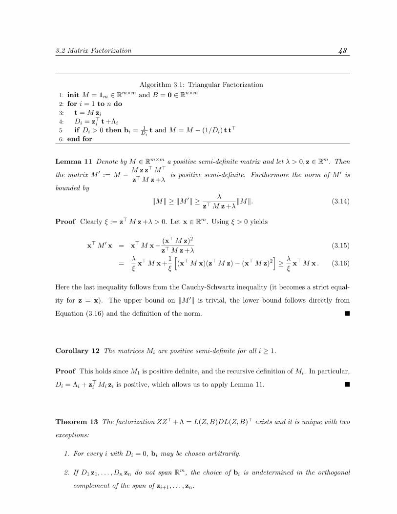
3.2 Matrix Factorization 43
Algorithm 3.1: Triangular Factorization1: init M = 1m ∈ Rm×m and B = 0 ∈ Rn×m
2: for i = 1 to n do3: t = M zi
4: Di = z>i t+Λi
5: if Di > 0 then bi = 1Di
t and M = M − (1/Di) t t>
6: end for
Lemma 11 Denote by M ∈ Rm×m a positive semi-definite matrix and let λ > 0, z ∈ Rm. Then
the matrix M ′ := M − M z z>M>
z>M z+λis positive semi-definite. Furthermore the norm of M ′ is
bounded by
‖M‖ ≥ ‖M ′‖ ≥ λ
z>M z+λ‖M‖. (3.14)
Proof Clearly ξ := z>M z+λ > 0. Let x ∈ Rm. Using ξ > 0 yields
x>M ′ x = x>M x− (x>M z)2
z>M z+λ(3.15)
=λ
ξx>M x+
1ξ
[(x>M x)(z>M z)− (x>M z)2
]≥ λ
ξx>M x . (3.16)
Here the last inequality follows from the Cauchy-Schwartz inequality (it becomes a strict equal-
ity for z = x). The upper bound on ‖M ′‖ is trivial, the lower bound follows directly from
Equation (3.16) and the definition of the norm.
Corollary 12 The matrices Mi are positive semi-definite for all i ≥ 1.
Proof This holds since M1 is positive definite, and the recursive definition of Mi. In particular,
Di = Λi + z>i Mi zi is positive, which allows us to apply Lemma 11.
Theorem 13 The factorization ZZ>+Λ = L(Z,B)DL(Z,B)> exists and it is unique with two
exceptions:
1. For every i with Di = 0, bi may be chosen arbitrarily.
2. If D1 z1, . . . , Dn zn do not span Rm, the choice of bi is undetermined in the orthogonal
complement of the span of zi+1, . . . , zn.
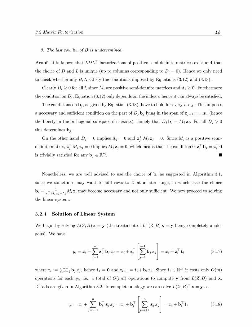
3.2 Matrix Factorization 44
3. The last row bn of B is undetermined.
Proof It is known that LDL> factorizations of positive semi-definite matrices exist and that
the choice of D and L is unique (up to columns corresponding to Di = 0). Hence we only need
to check whether any B,Λ satisfy the conditions imposed by Equations (3.12) and (3.13).
Clearly Di ≥ 0 for all i, since Mi are positive semi-definite matrices and Λi ≥ 0. Furthermore
the condition onDi, Equation (3.12) only depends on the index i, hence it can always be satisfied.
The conditions on bj , as given by Equation (3.13), have to hold for every i > j. This imposes
a necessary and sufficient condition on the part of Dj bj lying in the span of zj+1, . . . , zn (hence
the liberty in the orthogonal subspace if it exists), namely that Dj bj = Mj zj . For all Dj > 0
this determines bj .
On the other hand Dj = 0 implies Λj = 0 and z>j Mj zj = 0. Since Mj is a positive semi-
definite matrix, z>j Mj zj = 0 implies Mj zj = 0, which means that the condition 0 ·z>i bj = z>i 0
is trivially satisfied for any bj ∈ Rm.
Nonetheless, we are well advised to use the choice of bi as suggested in Algorithm 3.1,
since we sometimes may want to add rows to Z at a later stage, in which case the choice
bi = 1z>i Mi zi +Λi
Mi zi may become necessary and not only sufficient. We now proceed to solving
the linear system.
3.2.4 Solution of Linear System
We begin by solving L(Z,B)x = y (the treatment of L>(Z,B)x = y being completely analo-
gous). We have
yi = xi +i−1∑j=1
z>i bj xj = xi + z>i
i−1∑j=1
bj xj
= xi + z>i ti (3.17)
where ti :=∑i−1
j=1 bj xj , hence t1 = 0 and ti+1 = ti +bi xi. Since ti ∈ Rm it costs only O(m)
operations for each yi, i.e., a total of O(mn) operations to compute y from L(Z,B) and x.
Details are given in Algorithm 3.2. In complete analogy we can solve L(Z,B)> x = y as
yi = xi +n∑
j=i+1
b>i zj xj = xi + b>i
n∑j=i+1
zj xj
= xi + b>i ti (3.18)
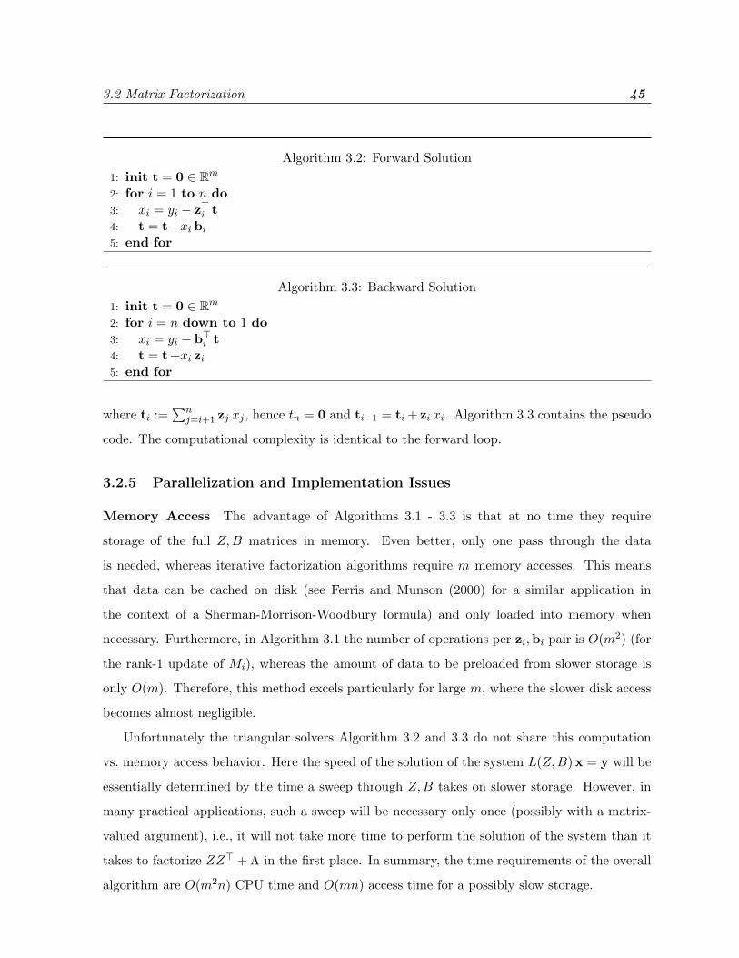
3.2 Matrix Factorization 45
Algorithm 3.2: Forward Solution1: init t = 0 ∈ Rm
2: for i = 1 to n do3: xi = yi − z>i t4: t = t+xi bi
5: end for
Algorithm 3.3: Backward Solution1: init t = 0 ∈ Rm
2: for i = n down to 1 do3: xi = yi − b>i t4: t = t+xi zi
5: end for
where ti :=∑n
j=i+1 zj xj , hence tn = 0 and ti−1 = ti + zi xi. Algorithm 3.3 contains the pseudo
code. The computational complexity is identical to the forward loop.
3.2.5 Parallelization and Implementation Issues
Memory Access The advantage of Algorithms 3.1 - 3.3 is that at no time they require
storage of the full Z,B matrices in memory. Even better, only one pass through the data
is needed, whereas iterative factorization algorithms require m memory accesses. This means
that data can be cached on disk (see Ferris and Munson (2000) for a similar application in
the context of a Sherman-Morrison-Woodbury formula) and only loaded into memory when
necessary. Furthermore, in Algorithm 3.1 the number of operations per zi,bi pair is O(m2) (for
the rank-1 update of Mi), whereas the amount of data to be preloaded from slower storage is
only O(m). Therefore, this method excels particularly for large m, where the slower disk access
becomes almost negligible.
Unfortunately the triangular solvers Algorithm 3.2 and 3.3 do not share this computation
vs. memory access behavior. Here the speed of the solution of the system L(Z,B)x = y will be
essentially determined by the time a sweep through Z,B takes on slower storage. However, in
many practical applications, such a sweep will be necessary only once (possibly with a matrix-
valued argument), i.e., it will not take more time to perform the solution of the system than it
takes to factorize ZZ> + Λ in the first place. In summary, the time requirements of the overall
algorithm are O(m2n) CPU time and O(mn) access time for a possibly slow storage.

3.2 Matrix Factorization 46
Parallelization In the following we assume that we have N nodes which are all directly con-
nected to each other and that there exist no preferred connections in the computer. Clearly
the main cost in Algorithm 3.1 for large systems is the rank-1 update M ← M − bi t>, as it
requires O(m2) operations and O(m2) storage. We can solve this problem by splitting M into
N stripes of m/N rows and distributing them onto the N nodes and performing scatter/gather
operations to distribute zi and collect t. Algorithm 3.4 contains the pseudo code. For conve-
nience we denote by Ml the lth stripe of M and by tl the corresponding stripe of t, as obtained
by tl = Ml zi.
Algorithm 3.4: Parallel Triangular Factorization1: init each node with a stripe Ml of M = 1m ∈ Rm×m
2: for i = 1 to n do3: master: broadcast to all slaves zi, Di
4: slave l: compute tl = Ml zi and λl := (zi)>l tl
5: slave l: broadcast tl and λl
6: slaves and master: receive tk and λk, assemble t, compute Di = Λi +∑N
k=1 λk
7: master: if Di > 0 bi = 1Di
t, else t = 08: master: record Di,bi to disk9: slave l: if Di > 0 update stripe Ml = Ml − (bi)l t>
10: end for
The bottleneck of Algorithm 3.4 is the broadcast and collection of tk. Here latencies of the
communications process will become the dominant factor (we assume that on most computers
the time for broadcasting a vector is small in comparison to the time to initiate the broadcast).
The remaining steps are non blocking, since storage of bi and broadcast of zi can be performed
asynchronously. Finally, similar considerations apply to the forward and backward solution of
the linear system.
3.2.6 Extensions
Several extensions of the above factorization can be obtained without much modification of the
original algorithm. Below we present a selection of them:
Modified Metric Straightforward calculus shows that we can use Algorithm 3.1 also to obtain
an efficient LDL> factorization of matrices such as A = Λ + ZMZ>, where M is an arbitrary
positive semi-definite matrix. All that is required is to set M1 = M instead of M1 = 1.

3.3 An LDV Factorization 47
Indefinite Diagonal Terms There is no inherent restriction why Λ should be a positive
matrix. Indeed, all that is required is that Λ + ZZ> be positive semi-definite such that an
LDL> decomposition exists. However, as pointed out in Fletcher and Powell (1974) for the case
of vectorial Z, numerical stability can suffer if this decomposition leads to Mi with very small
or spurious negative eigenvalues.
3.3 An LDV Factorization
The factorization algorithm for ZZ>+Λ can also be used to obtain an LDV factorization of Z,
simply by running the original factorization with Λ = 0 and converting the obtained factorization
into an LDV factorization. Here L is a lower triangular matrix, D is diagonal, and V satisfies
V >DV = 1m. We extend a result from Gill et al. (1975).
Lemma 14 The factorization defined by Equation (3.7) satisfies LDB = Z.
Proof With the definition of L(Z,B) and using the fact that M> = M and D> = D we can
rewrite LDB = Z row-wise as
z>i = Di b>i +i−1∑j=1
z>i bj Dj b>j = Di b>i + z>i
i−1∑j=1
bj Dj b>j
⇐⇒ biDi = Mi zi .
The latter condition, however, is identical with the implications of Equation (3.13), hence the
claim is proven.
What this means is that if we use the LDL> factorization algorithm on the matrix ZZ> +
0 we will obtain the decomposition LDB = Z. All we need to argue is that the resulting
matrices L,D,B can be easily converted into an LDV factorization. The pseudo code is given
in Algorithm 3.5. For its analysis we need an auxiliary lemma.
Lemma 15 The image of 1m−Mi+1 is contained in span{z1, . . . , zi}. Furthermore ziMi zi = 0
implies zi ∈ span{z1, . . . , zi−1}.
Proof We use induction: for the first claim recall that 1m−M1 = 0, hence the induction
assumption holds. Next note that Mi+1 = Mi − cMi zi z>i Mi with c ≥ 0. Since we know the
image of 1m−Mi we only need to study Mi zi z>i Mi to contain the image of 1m−Mi+1.
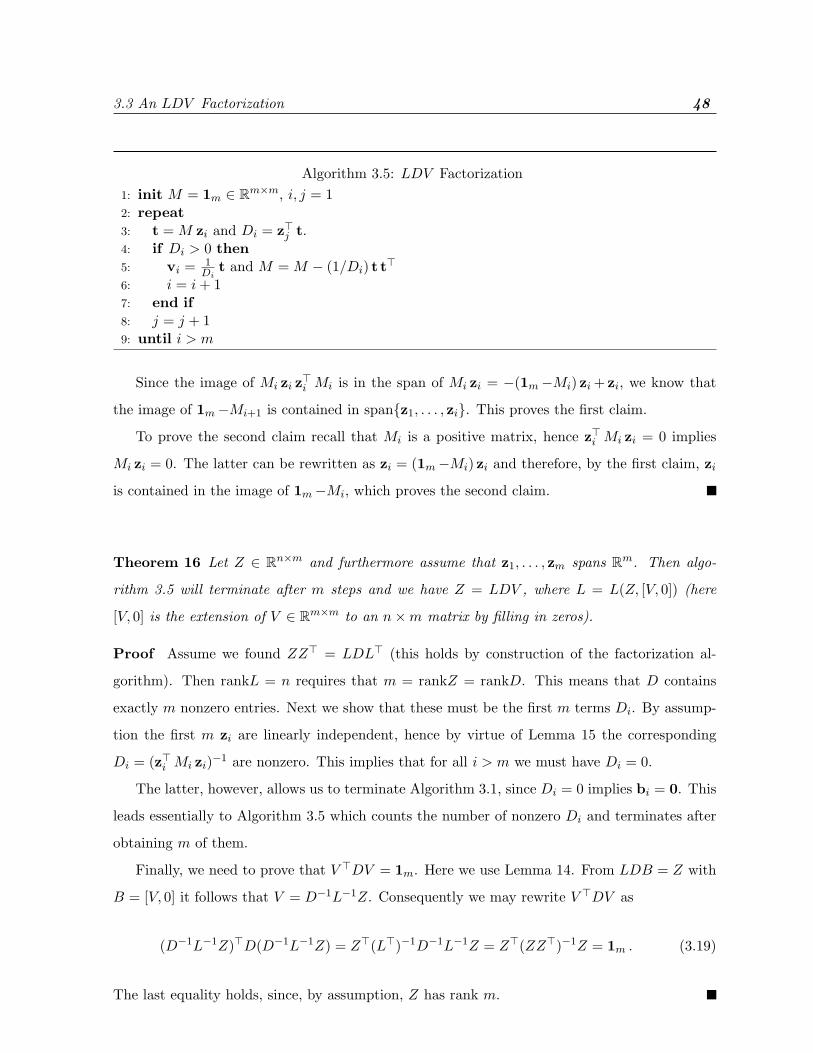
3.3 An LDV Factorization 48
Algorithm 3.5: LDV Factorization1: init M = 1m ∈ Rm×m, i, j = 12: repeat3: t = M zi and Di = z>j t.4: if Di > 0 then5: vi = 1
Dit and M = M − (1/Di) t t>
6: i = i+ 17: end if8: j = j + 19: until i > m
Since the image of Mi zi z>i Mi is in the span of Mi zi = −(1m−Mi) zi + zi, we know that
the image of 1m−Mi+1 is contained in span{z1, . . . , zi}. This proves the first claim.
To prove the second claim recall that Mi is a positive matrix, hence z>i Mi zi = 0 implies
Mi zi = 0. The latter can be rewritten as zi = (1m−Mi) zi and therefore, by the first claim, zi
is contained in the image of 1m−Mi, which proves the second claim.
Theorem 16 Let Z ∈ Rn×m and furthermore assume that z1, . . . , zm spans Rm. Then algo-
rithm 3.5 will terminate after m steps and we have Z = LDV , where L = L(Z, [V, 0]) (here
[V, 0] is the extension of V ∈ Rm×m to an n×m matrix by filling in zeros).
Proof Assume we found ZZ> = LDL> (this holds by construction of the factorization al-
gorithm). Then rankL = n requires that m = rankZ = rankD. This means that D contains
exactly m nonzero entries. Next we show that these must be the first m terms Di. By assump-
tion the first m zi are linearly independent, hence by virtue of Lemma 15 the corresponding
Di = (z>i Mi zi)−1 are nonzero. This implies that for all i > m we must have Di = 0.
The latter, however, allows us to terminate Algorithm 3.1, since Di = 0 implies bi = 0. This
leads essentially to Algorithm 3.5 which counts the number of nonzero Di and terminates after
obtaining m of them.
Finally, we need to prove that V >DV = 1m. Here we use Lemma 14. From LDB = Z with
B = [V, 0] it follows that V = D−1L−1Z. Consequently we may rewrite V >DV as
(D−1L−1Z)>D(D−1L−1Z) = Z>(L>)−1D−1L−1Z = Z>(ZZ>)−1Z = 1m . (3.19)
The last equality holds, since, by assumption, Z has rank m.
3.4 Rank Modifications 49
If the first m zi are linearly dependent, the algorithm will iterate until it has found a set
of m linearly independent zi to construct the decomposition. Note that we are able to find an
implicit representation of the LDV decomposition in O(m3) time which can be much less than
the time required to visit all entries of Z.2
3.4 Rank Modifications
Now that we presented an algorithm to factorize ZZ> + D into LDL>, we study how such a
factorization can be useful in dealing with modifications of the original equation into
ZZ> + Λ + pp> = L D L> (3.20)
with corresponding B. To address this problem we will distinguish between three different
cases: (1) p is an arbitrary vector, (2) p can be written as p = Z q, (3) we want to modify
Equation (3.7) by removing the ith row and column. It will turn out that (3) can be essentially
reduced to (2).
The general idea of what follows is that we will be able to compute D efficiently without
knowing B and only subsequently compute B via D and an implicit formulation for L. Note
that the methods presented in the following could be easily adapted to rank modifications of an
LDV decomposition of an arbitrary matrix Z.
3.4.1 Generic Rank-1 Update
Consider Equation (3.20), knowing that ZZ> + Λ = LDL> we can rewrite it as
D + aa> = L−1 L D L>(L−1)> (3.21)
where, a := L−1 p can be computed in O(mn) time (see Algorithm 3.2). Moreover, we can find
a factorization L D L = D+ aa> in O(n) time by using Algorithm 3.1. If L = L(a,b) then it is
2Of course, to obtain the explicit values of L we would have to expend O(m2n) time. However, this is oftennot needed, when L is only used to find pseudo-inverses.

3.4 Rank Modifications 50
clear that b = D−1
L−1
a. We also observe that
L D L = L L D LL> hence D = D and L = L L . (3.22)
This follows from the uniqueness of LDL> decompositions (recall that the product of two lower
triangular matrices is a lower triangular matrix). To compute B we introduce Z := [Z,p].
Application of Lemma 14 yields
LDB = Z and L D B = Z = [Z,p] = [LDB,p] (3.23)
hence B = D−1 L−1[LDB,p] = D−1
L−1
[DB,a] = [D−1
L−1DB,b]. Note that L
−1DB can
be computed in O(mn) time since L−1
x for some x ∈ Rn can be computed in O(n) time. In
summary, we obtain a generic rank-1 update by computing a = L−1 p, then factorize D+ aa>,
yielding L D L>, and finally compute B = [D
−1L−1DB,b].
3.4.2 Rank-1 Update Where p = Z q
Here we may rewrite Equation (3.20) as
ZZ> + Λ + pp> = Z(1m +qq>)Z> + Λ = Z Z> +Λ (3.24)
where Z := Zχ and χ := (1m +qq>)12 . This means that we can apply Lemma 14 to the L D L>
decomposition of Equation (3.20) to obtain
L D B = Z = Zχ = LDBχ and hence B = D−1 L−1LDBχ. (3.25)
Next note that L−1 p = L−1Z q = DB q. This allows us to rewrite Equation (3.21) as
D + (L−1 p)(L−1 p)> = D +DB qq>B>D = L−1 L D L>(L−1)>. (3.26)
Here D and L can be found in O(n) time. By the same reasoning as in Section 3.4.1 we obtain
L = LL and D = D. This leads to
B = D−1 L−1LDBχ = D−1 L
−1DBχ. (3.27)
3.4 Rank Modifications 51
The key point to note is that here B gives us a factorization of L via L(Z, B), which is not quite
desirable, since it means that we would have to update not only B but also Z. However, B, Z
only appear in the form of dot products via z>i bj = z>i χbj . This means that we can keep Z, if
we multiply B by χ. In summary we obtain
Bfinal = Bχ = D−1 L−1DB(1m +qq>). (3.28)
Each of the steps can be carried out in O(mn) time, which determines the complexity of the
algorithm (note that we can gain a slight improvement by carrying out D−1 L−1D in one step).
3.4.3 Removal of a Row and Column
Assume that we have a factorization of ZZ>+Λ = LDL> and we would like to find a factoriza-
tion of ZZ>+Λ efficiently, where Z, Λ have been obtained by removing the i-th row (and column
respectively). It is well known (see e.g., Golub and Loan (1996)) that by such a modification
only the “lower right” part of L will change. For the sake of completeness we briefly repeat the
reasoning below. We split Z,D,L,Λ into three parts as follows:
Z =
Z1
Z2
Z3
Λ =
Λ1
Λ2
Λ3
D =
D1
D2
D3
L =
L11
L21 L22
L31 L32 L33
Likewise we have for the reduced system
Z =
Z1
Z3
Λ =
Λ1
Λ3
D =
D1
D3
L =
L11
L31 L33
Finally we decompose B, B in the same fashion. Matching up terms in the reduced system leads
to the equations
Z1Z>1 + Λ1 = L11D1L
>11 = L11D1L
>11
Z3Z>1 = L31D1L
>11 = L31D1L
>11
Z3Z>3 + Λ3 = L31D1L
>31 + L32D2L
>32 + L33D3L
>33 = L31D1L
>31 + L33D3L
>33.

3.5 Applications 52
The first two conditions of the system imply L11 = L11, D1 = D1, and L31 = L31. These
conditions on L can be satisfied by setting B1 = B1. Hence, we need to expend computational
effort only on satisfying
L32D2L>32 + L33D3L
>33 = L33D3L
>33. (3.29)
By the definition of L(Z,B) we know that L32 can be written as L32 = Z3B>2 , which leads to
Z3B>2 D2B2Z
>3 +L33D3L
>33 = L33D3L
>33. This problem, however, is identical to the one discussed
in Section 3.4.2 — simply substitute q = B2
√D2. This leads to the following update equations:
1. Factorize D3 +D3B3B>2 D2B2B
>3 D3 = L D L and set D3 = D, as in Equation (3.26).
2. Using Equation (3.28) compute B3 via B3 = D−13 L
−1D3B3(1m +B2D2B
>2 ).
Assuming that Z3 is an n′×m matrix (n′ = n−i), the first step only involves O(mn′) operations
to compute D3B3B>2
√D2 and O(n′) operations to compute L, D. Likewise, the second step costs
only O(mn′) operations (multiplication by a diagonal matrix, product with L−1
, rank-1 update
on B3).
3.5 Applications
3.5.1 Interior Point Methods
Our reasoning is similar to the one proposed in Goldfarb and Scheinberg (2001) and it presents
an alternative to Seol and Park (2002). In a nutshell the idea is the following: assume we want
to invert a matrix M which has the form M = ZZ> + C, where M,C ∈ Rn×n and Z ∈ Rn×m,
usually m � n, and finally C is easily invertible. Then the (numerically less stable) Sherman-
Morrison-Woodbury approach consists of replacing
(ZZ> + C)−1 x by[C−1 − C−1Z(Z>CZ + 1m)−1Z>C−1
]x . (3.30)
On the other hand, if we wish to find an LDL> factorization, we first factorize C into C =
LcDcL>c , which, by assumption, can be done cheaply. Subsequently, we factorize (L−1
c Z)(L−1c Z)>+
Dc = LzDzLz and make the replacement of
(ZZ> + C)−1 x by[LcLzDzL
>z L
>c
]−1x . (3.31)

3.5 Applications 53
Such a situation may occur in several cases:
Rank Degenerate Quadratic Objective Function In a quadratic programming problem
with objective function f(x) = x>H x+ c> x, where H has only rank m, or where it can be
approximated by a low-rank matrix (Ferris and Munson, 2000, Scholkopf and Smola, 2002, Fine
and Scheinberg, 2001), interior point codes lead to the following linear system (Vanderbei, 1994):
−(ZZ> +D) A
A> Hy
x
y
=
cx
cy
(3.32)
Here H = ZZ> (or H ≈ ZZ> in case we use a low-rank approximation of H) and D is a
diagonal matrix with positive entries. Equation (3.32) is typically solved by explicit pivoting for
the upper left block, which involves computing
(ZZ> +D)−1A and (ZZ> +D)−1 cx . (3.33)
Even if Z is a triangular matrix, it is difficult to invert (ZZ>+D)−1 and provides a picture-book
case of where our factorization can be applied (in fact, this was the reason for our derivations).
Dense Columns Linear programming involves solving a linear system (Vanderbei, 1997) sim-
ilar to Equation (3.32): −D A
A> 0
x
y
=
cx
cy
(3.34)
Here A represents the matrix of constraints, and D is a positive diagonal matrix. Typically
Equation (3.34) is solved by explicit pivoting for x, which leads to
x = D−1Ay−D−1cx and (A>D−1A)y = cy +A>D−1cx. (3.35)
If A is largely a sparse matrix with a few dense columns, Equation (3.35) nonetheless amounts
to solving a dense system. To avoid such problems we assume that A can be decomposed into
A = [Ad, As] (and likewise D into Dd and Ds) where Ad represents the dense columns and
As corresponds to the sparse ones (to keep the notation simple, for the purpose of the exam-
ple we assume that AdD−1d Ad has full rank). This means that we need solve linear systems
3.5 Applications 54
involving A>s D−1s As +A>d D
−1d Ad. Here as in Equation (3.31), we assume that an L D L
>factor-
ization for A>s D−1s As can be obtained efficiently, and a subsequent application of our method
to L−1A>d DdAd(L
−1)> + D yields the factorization of A>D−1A.
3.5.2 Lazy Decomposition
Recall the original problem Equation (3.2) of factorizing ZZ>+Λ. Frequently Λ will have large
entries (more specifically Λi � ‖ zi ‖2). In such cases it intuitively makes sense to “ignore” the
contribution of zi and save computational time by considering only Λi. In the following we will
formalize this notion.
Lemma 17 Assume that Mi is given by Algorithm 3.1. Then
0 ≤ a>Mi a−a>Mi+1 aa>Mi+1 a
≤ z>i Mi zi
Λifor all a ∈ Rm, i ∈ N . (3.36)
Proof The LHS of Equation (3.36) is trivial, since Mi −Mi+1 = αqq> for suitable α > 0 and
z ∈ Rm. To show the RHS we use
a>Mi a>−a>Mi+1 aa>Mi+1 a
=(a>Mi zi)2
(Λi + z>i Mi zi)a>Mi a−(a>Mi zi)2(3.37)
≤ (a>Mi zi)2
Λi a>Mi a≤ z>i Mi zi
Λi. (3.38)
Here the last two inequalities followed from the Cauchy-Schwartz inequality, i.e., that (a>M b)2 ≤
a>M ab>M b for any positive matrix M .
If the changes in Mi are smaller than the error tolerance, say z>i Mi zi
Λi≤ ε, we may decide
not to carry out the update on Mi at all (e.g., they would be smaller than the numerical error
introduced by the operation). Furthermore, note that M1 = 1m, hence M1 z = z. Now assume
that we reordered the rows/columns of ZZ> + Λ in such a way that the entries corresponding
to ‖ zi ‖2 > εΛi occur first. Then, for all such zi, no update in Mi will be carried out. Moreover,
Mi zi = zi, which again does not involve computational cost. Finally, we set bi = 1‖ zi ‖2+Λi
zi.
In a nutshell, this means that we can perform each of those steps at O(n) rather than O(n2)
cost, which leads to a significant speedup if such a situation happens for a large number of zi.
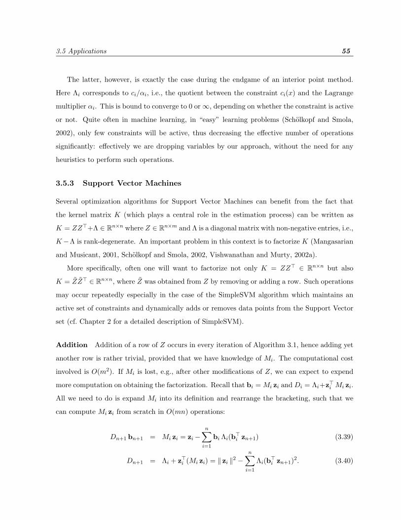
3.5 Applications 55
The latter, however, is exactly the case during the endgame of an interior point method.
Here Λi corresponds to ci/αi, i.e., the quotient between the constraint ci(x) and the Lagrange
multiplier αi. This is bound to converge to 0 or∞, depending on whether the constraint is active
or not. Quite often in machine learning, in “easy” learning problems (Scholkopf and Smola,
2002), only few constraints will be active, thus decreasing the effective number of operations
significantly: effectively we are dropping variables by our approach, without the need for any
heuristics to perform such operations.
3.5.3 Support Vector Machines
Several optimization algorithms for Support Vector Machines can benefit from the fact that
the kernel matrix K (which plays a central role in the estimation process) can be written as
K = ZZ>+Λ ∈ Rn×n where Z ∈ Rn×m and Λ is a diagonal matrix with non-negative entries, i.e.,
K−Λ is rank-degenerate. An important problem in this context is to factorize K (Mangasarian
and Musicant, 2001, Scholkopf and Smola, 2002, Vishwanathan and Murty, 2002a).
More specifically, often one will want to factorize not only K = ZZ> ∈ Rn×n but also
K = ZZ> ∈ Rn×n, where Z was obtained from Z by removing or adding a row. Such operations
may occur repeatedly especially in the case of the SimpleSVM algorithm which maintains an
active set of constraints and dynamically adds or removes data points from the Support Vector
set (cf. Chapter 2 for a detailed description of SimpleSVM).
Addition Addition of a row of Z occurs in every iteration of Algorithm 3.1, hence adding yet
another row is rather trivial, provided that we have knowledge of Mi. The computational cost
involved is O(m2). If Mi is lost, e.g., after other modifications of Z, we can expect to expend
more computation on obtaining the factorization. Recall that bi = Mi zi and Di = Λi+z>i Mi zi.
All we need to do is expand Mi into its definition and rearrange the bracketing, such that we
can compute Mi zi from scratch in O(mn) operations:
Dn+1 bn+1 = Mi zi = zi−n∑
i=1
bi Λi(b>i zn+1) (3.39)
Dn+1 = Λi + z>i (Mi zi) = ‖ zi ‖2 −n∑
i=1
Λi(b>i zn+1)2. (3.40)
3.6 Summary 56
The proposed factorization is faster than a direct method O(n2) operations, as used in algorithms
like those proposed by Cauwenberghs and Poggio (2001).
Removal Here we can use the results from Section 3.4.3 concerning the rank-1 modification
of a matrix by removal of a row and column. Unlike the Cauwenberghs and Poggio (2001)
algorithm, which expends O(n2) effort on that, we can perform such operations now in O(mn)
time, a significant computational advantage, given the fact that often m� n.
3.6 Summary
We presented a fast algorithm for computing the Cholesky decomposition of a class of matrices
which occur frequently in machine learning applications. We discussed strategies for parallel
implementation. Rank one updates to the factorization were also derived. We demonstrated
the use of our factorization in speeding up the SimpleSVM algorithm as well as interior point
methods. Error analysis of the proposed factorization along the lines of Bennett (1965) is a
topic of current research.

Chapter 4
Kernels on Discrete Objects
In this chapter we provide a general overview of R-Convolution kernels proposed by Haussler
(1999). We produce many extensions and exhibit new kernels and also show how various previous
kernels can be viewed in this framework. The aim of this chapter is to provide general recipes
for defining kernels on strings, trees, Finite State Automata, images, etc. A few fast algorithms
for computing kernels on sets are sketched in this chapter. Specific implementation details and
fast real life algorithms of all other kernels are relegated to later chapters.
This chapter is organized as follows. In Section 4.1 we motivate the need for kernels on
discrete objects and present various applications. We go on to survey some recent literature on
kernels for strings and trees. We review some basic concepts of convolution kernels and discuss
our extensions in Section 4.2. In Section 4.3 we discuss kernels on sets, in Section 4.4 we discuss
kernels on strings, in Section 4.5 we discuss kernels on trees, in Section 4.6 we discuss kernels
on Automata. and finally in Section 4.7 we define novel kernels on images.
This chapter requires the reader to understand the notion of a kernel. Review of Section 1.3
may be helpful. This chapter is a pre-requisite for reading Chapters 5 and 6. Readers may want
to read the influential paper by Haussler (1999) to gain a deeper understanding of convolution
kernels and their extensions presented in this chapter. Knowledge of different types of Automata
may be useful in understanding material presented in Section 4.6. We refer the reader to the
authoritative text by Hopcroft and Ullman (1979) for further details.
57

4.1 Introduction 58
4.1 Introduction
Many problems in machine learning require the classifier to work with a set of discrete examples.
Common examples are biological sequence analysis where data is represented as strings (Durbin
et al., 1998), Natural Language Processing (NLP) where the data is in the form of a parse tree
(Collins and Duffy, 2001), Internet connectivity where the connections are denoted by graphs
(Kondor and Lafferty, 2002). In order to apply machine learning algorithms on such discrete
data it is desirable to have a function of similarity. This can be achieved by the use of a feature
mapping of the form φ : X → HK where X is the set of discrete structures (for eg. the set of all
parse trees of a language) and HK is some Hilbert space. Furthermore, dot products in Hilbert
spaces lead to kernels
k(x, x′) = 〈φ(x), φ(x′)〉, (4.1)
where x, x′ ∈ X . It is clear that the success of kernel methods depends upon a faithful repre-
sentation of discrete data that can be computed efficiently. It should take into account both
the content as well as the inherent structural information present in the data. These notions of
similarity can also be extended to other areas like information retrieval and bio-informatics in a
natural and intuitive way.
4.1.1 Applications of Kernels on Discrete Structures
Kernels on discrete structures are very useful in a wide variety of fields.
Bio-Informatics Kernels on strings are widely used in the field of bio-informatics to compare
the similarity between two DNA sequences and for protein homology detection (Leslie
et al., 2002a,b, Jaakkola et al., 1999).
Intrusion Detection Use of the spectrum kernel for analyzing the system call traces in order
to detect intrusions can be found in Eskin et al. (2001). Other kinds of network data
including network logs can be analyzed effectively using a string kernel.
Natural Language Processing Use of kernels for defining similarity between parse trees has
been studied in Collins and Duffy (2001).
Document Retrieval on the Web Search engines have to deal with a lot of unstructured
data which is available in a wide variety of formats on the web. It is useful to have some

4.1 Introduction 59
algorithm by which measures of similarity can be computed for such documents (Joachims,
2002, Manevitz and Yousef, 2001).
Structured Text In the field of information retrieval, string kernels are very useful in order
to define a similarity metric between text documents or web pages (Lodhi et al., 2002).
The structure of XML and HTML documents can also be utilized to define a meaningful
similarity metric (Joachims et al., 2001).
Images Comparing two images for similarity has always been a hard problem. It is compounded
by the fact that the same image at two different scales has two different representations. A
possible way to get around this problem is to use image segmentation techniques in order to
decompose the image into a tree like structure and then compare the similarities between
them. Another method is to encode all rectangular regions of an image into a compact
data structure and compare two images based on the number of rectangular regions they
share (cf. Section 4.7 for more details).
4.1.2 Previous Work
Recently convolution kernels proposed by Haussler (1999) have gained prominence in the field of
machine learning. They are obtained from other kernels by a certain sum over products which
can be viewed as a generalized convolution. The advantage of these kernels is that they can be
applied iteratively to build a kernel on more complex structures by using the kernels defined on
its components.
Pair HMM’s were first introduced for biological sequence analysis by Durbin et al. (1998).
A pair HMM is essentially a HMM that generates two symbol sequences simultaneously. Thus,
it defines a joint probability distribution over finite symbol sequences. The dynamic alignment
kernel algorithm uses a pair HMM to define a kernel (Watkins, 2000). Given a pair of strings
the dynamic alignment kernel is defined as the probability that the pair of strings was emitted
by the pair HMM.
Kernels on strings were motivated by the work of Haussler (1999) and Watkins (2000).
Explicit recursion formulas for calculation of various string kernels can be found in Herbrich
(2002). Various weighing schemes like the inverse-document-frequency (IDF) or cosine functions
which are widely used in information retrieval can also be incorporated into string kernels to
increase their relevance. A special case of the string kernel is the k-spectrum kernel defined
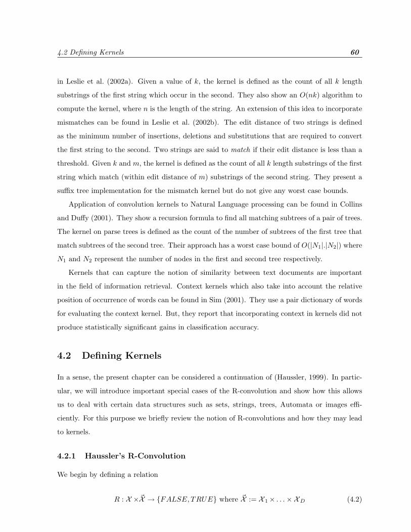
4.2 Defining Kernels 60
in Leslie et al. (2002a). Given a value of k, the kernel is defined as the count of all k length
substrings of the first string which occur in the second. They also show an O(nk) algorithm to
compute the kernel, where n is the length of the string. An extension of this idea to incorporate
mismatches can be found in Leslie et al. (2002b). The edit distance of two strings is defined
as the minimum number of insertions, deletions and substitutions that are required to convert
the first string to the second. Two strings are said to match if their edit distance is less than a
threshold. Given k and m, the kernel is defined as the count of all k length substrings of the first
string which match (within edit distance of m) substrings of the second string. They present a
suffix tree implementation for the mismatch kernel but do not give any worst case bounds.
Application of convolution kernels to Natural Language processing can be found in Collins
and Duffy (2001). They show a recursion formula to find all matching subtrees of a pair of trees.
The kernel on parse trees is defined as the count of the number of subtrees of the first tree that
match subtrees of the second tree. Their approach has a worst case bound of O(|N1|.|N2|) where
N1 and N2 represent the number of nodes in the first and second tree respectively.
Kernels that can capture the notion of similarity between text documents are important
in the field of information retrieval. Context kernels which also take into account the relative
position of occurrence of words can be found in Sim (2001). They use a pair dictionary of words
for evaluating the context kernel. But, they report that incorporating context in kernels did not
produce statistically significant gains in classification accuracy.
4.2 Defining Kernels
In a sense, the present chapter can be considered a continuation of (Haussler, 1999). In partic-
ular, we will introduce important special cases of the R-convolution and show how this allows
us to deal with certain data structures such as sets, strings, trees, Automata or images effi-
ciently. For this purpose we briefly review the notion of R-convolutions and how they may lead
to kernels.
4.2.1 Haussler’s R-Convolution
We begin by defining a relation
R : X ×~X → {FALSE, TRUE} where ~X := X 1× . . .×XD (4.2)

4.2 Defining Kernels 61
or in short R(x,x), where the xi with (x1, . . . , xD) ∈ ~X are considered to be the “parts” of x.
This allows us to consider the sets
R−1(x) := {x |R(x,x) = TRUE}. (4.3)
In particular, we assume, following Haussler (1999), that |R−1(x)| is countable. However, we use
a slight extension, namely that R−1(x) may be a multi-set, i.e., it may contain elements more
than once. For instance, a text might contain the word ”dog” several times. This modification
greatly simplifies the subsequent considerations concerning exact and inexact matches. Next,
we introduce the R-convolution of the kernels k1, . . . , kD with ki : X i×X i → R via
k1 ? . . . ? kD(x,x′) :=∑
x∈R−1(x)
x′∈R−1(x′)
k1(x1, x′1) · . . . · kD(xD, x
′D). (4.4)
Depending on the definitions of R and ki we obtain a very rich class of kernels. In particular,
we may use recursive versions of Equation (4.4) to define kernels on objects such as trees. See
(Haussler, 1999, Section 2.2 and 4) for details and examples.
4.2.2 Exact and Inexact Matches
One theme will be central to our considerations: the difference between exact and inexact
matches. We call a kernel an exactly matching kernel if
k1 ? . . . ? kD(x,x′) :=∑
x∈R−1(x)
x′∈R−1(x′)
k1(x1, x′1) · . . . · kD(xD, x
′D)δx,x′ . (4.5)
Note that Equation (4.5) does not allow us to replace the double sum over R−1(x) and R−1(x′)
by a simple sum due to the fact that x might occur several times in R−1(x) (and likewise x′
in R−1(x′)). However, as may be apparent already now, significant computational gains can be
made in evaluating Equation (4.5) by sorting R−1(x) for each x beforehand and subsequently
comparing the sorted sets. While the specific form of sorting will depend on the kind of R we are
dealing with, it is safe to say that the central idea to efficient computation of exactly matching
kernels can be found in sorting the sets R−1(x) before evaluating Equation (4.5).
Concerning inexact matches, that is, the general case of Equation (4.4), it is safe to say
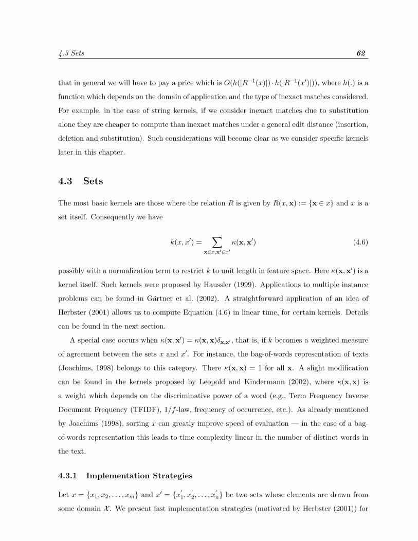
4.3 Sets 62
that in general we will have to pay a price which is O(h(|R−1(x)|) ·h(|R−1(x′)|)), where h(.) is a
function which depends on the domain of application and the type of inexact matches considered.
For example, in the case of string kernels, if we consider inexact matches due to substitution
alone they are cheaper to compute than inexact matches under a general edit distance (insertion,
deletion and substitution). Such considerations will become clear as we consider specific kernels
later in this chapter.
4.3 Sets
The most basic kernels are those where the relation R is given by R(x,x) := {x ∈ x} and x is a
set itself. Consequently we have
k(x, x′) =∑
x∈x,x′∈x′
κ(x,x′) (4.6)
possibly with a normalization term to restrict k to unit length in feature space. Here κ(x,x′) is a
kernel itself. Such kernels were proposed by Haussler (1999). Applications to multiple instance
problems can be found in Gartner et al. (2002). A straightforward application of an idea of
Herbster (2001) allows us to compute Equation (4.6) in linear time, for certain kernels. Details
can be found in the next section.
A special case occurs when κ(x,x′) = κ(x,x)δx,x′ , that is, if k becomes a weighted measure
of agreement between the sets x and x′. For instance, the bag-of-words representation of texts
(Joachims, 1998) belongs to this category. There κ(x,x) = 1 for all x. A slight modification
can be found in the kernels proposed by Leopold and Kindermann (2002), where κ(x,x) is
a weight which depends on the discriminative power of a word (e.g., Term Frequency Inverse
Document Frequency (TFIDF), 1/f -law, frequency of occurrence, etc.). As already mentioned
by Joachims (1998), sorting x can greatly improve speed of evaluation — in the case of a bag-
of-words representation this leads to time complexity linear in the number of distinct words in
the text.
4.3.1 Implementation Strategies
Let x = {x1, x2, . . . , xm} and x′ = {x′1, x′2, . . . , x
′n} be two sets whose elements are drawn from
some domain X . We present fast implementation strategies (motivated by Herbster (2001)) for

4.4 Strings 63
the set kernel defined as follows
k(x, x′) =∑xi∈x
∑x′j∈x′
K(xi, x′j), (4.7)
where K(., .) is a valid kernel function.
Suppose, we can write K(xi, x′j) as K(xi, x
′j) = ρ(xi)φ(x
′j) for some ρ(.) and φ(.) then from
Equation (4.7) we get
k(x, x′) =∑xi∈x
∑x′j∈x′
ρ(xi) · φ(x′j) =
∑xi∈x
ρ(xi) ·∑
x′j∈x′
φ(x′j)
which can be computed in O(m + n) time. Examples of such kernels include K(xi, x′j) = xix
′j
and K(xi, x′j) = exp−σ(xi−x
′j) for X = R.
Assume that, X = R and that the sets x and x′ are in ascending order 1, and let K(xi, x′j) =
exp−σ|xi−x′j |. Define, l[i] :=
∑ij=1 expσxj and r[i] =
∑mj=i+1 exp−σxj for 1 ≤ i ≤ m. For x
′j ∈ x′
define j∗ = max{i : xi ≤ x′j}. Now, we can compute k(x, x′) as
k(x, x′) =n∑
j=1
l[j∗] exp−σx′j +r[j∗] expσx
′j .
Computation of l[i] and r[i] for all i ∈ {1, 2, . . . ,m} takes O(m) time while j∗ for all j ∈
{1, 2, . . . , n} can be computed in O(m + n) time by merging x and x′. Thus, k(x, x′) can be
computed in O(m+ n) total time.
4.4 Strings
Strings occur naturally in many applications including information retrieval, web-document
retrieval, search engines and bio-informatics. The strings in such applications may contain
millions of characters and hence the speed of kernel evaluation is critical. We define various
kernels on strings in this section and show their relation to many previously defined kernels.
1If they are not in sorted order we can sort them by expending O(m log(m) + n log(n)) effort
4.4 Strings 64
4.4.1 Notation
Our notation for strings closely follows (Giegerich and Kurtz, 1997). Let A be a finite set which
we call the alphabet. The elements of A are characters. Let $ be a sentinel character such that
$ /∈ A. Any x ∈ Ak for k = 0, 1, 2 . . . is called a string. The empty string is denoted by ε. Some
examples of valid strings include
• Texts written in English defined over the alphabet A = {a, b, . . . , z, 0, 1, . . . , 9,�} (�
denotes the blank character)
• DNA sequences defined over the alphabet A = {A,C,G, T}
• Binary sequences defined over the alphabet A = {0, 1}
A∗ represents the set of all strings defined over the alphabet A. We denote by A+ the set of all
non empty strings defined over A. It is clear that A+ = A∗ \ε.
We use s, t, u, v, w, x, y to denote strings over the alphabet A and a, b, c to denote elements
of the alphabet. |x| denotes the length of string x. Concatenation of two strings u and v is
denoted by uv while concatenation of a character a to a string u is denoted by au. Given a
string t = t1t2 . . . tn where ti ∈ A, the reverse string is defined as t−1 := tn . . . t2t1. We use the
shorthand notation x[i : j] to define a substring of x between locations i and j (both inclusive)
where 1 ≤ i, j ≤ |x|. If x = uvw for some ( possibly empty ) u, v, w, then u is called a prefix
of x while v is called a substring and w is called a suffix of x. We sometimes use the notation
s v x to denote that s is a substring of x. A suffix or prefix of a string x is called nested if
it occurs elsewhere in x. Given two strings x and y, numy(x) denotes the number of times y
occurs as a substring of x.
4.4.2 Various String Kernels
It is immediately obvious that a simple frequency-of-occurrence count, such as in the bag-
of-words representation of texts discards a large amount of information inherent in a text.
Indeed, inclusion of a larger context of symbols can improve the generalization performance of
kernel methods (Sim, 2001, Lodhi et al., 2002). If we do not consider the contribution of gappy
substrings all currently used string kernels can be described in the following way:
k(x, x′) =∑
svx,s′vx′
κ(s, s′) (4.8)

4.4 Strings 65
where s, s′, x, x′ ∈ S are strings and s v x denotes that s is a substring of x. The following
special cases are worth considering.
Bag of Symbols: Here we have
κ(s, s′) =
wsδs,s′ if s ∈ A
0 otherwise
where ws are arbitrary nonnegative weights. In other words, only the frequency of occur-
rence of single symbols counts.
Bag of Substrings: To include context we extend the bag-of-words to a bag-of-substrings rep-
resentation. This means that we have a kernel of type
κ(s, s′) = wsδs,s′ .
Clearly the number of such substrings can be large (worst case it can be quadratic in the
length of x). This means that a naive implementation could take up to O(|x|2|x′|2) time to
compute k(x, x′), where |x| denotes the length of x. Chapter 5 will present an algorithm
which scales as O(|x| + |x′|), thus significantly improving on previous algorithms which
were of order O(|x| · |x′|) (see e.g., Herbrich (2002) for an overview). A special case of this
kernel is the length weighted kernel which uses
ws = λ|s|
where λ is a weighing factor. λ > 1 means that longer substring matches are favored while
λ < 1 favors smaller substring matches. Another special case takes into account substrings
of length greater than a given threshold and is given by
κ(s, s′) = wsδs,s′δ(|s| > T )
where T is the given threshold on the length of the substrings that match. An alternate
way of looking at it is to set ws = 0 if |s| < T . This may be useful in information retrieval
applications where we do not want frequently occurring connectors like a, an, the, etc. to
contribute to the kernel value.

4.5 Trees 66
The kernels proposed by Leslie et al. (2002a,b), Haussler (1999), Watkins (2000) are a special
case of our definitions and the algorithm we present in Chapter 5 will contain the previous
methods as a special case or be significantly faster than the originally proposed strategies.
4.5 Trees
Trees are widely used data structures for searching and database operations. They also occur
frequently in many applications including Natural Language Processing and database searching.
We define various kernels on trees in this section and show their relation to many previously
defined kernels. We also propose a way to handle inexact matches by using coarsening levels in
trees.
4.5.1 Notation
A tree is defined as a connected graph with no cycles. The set of nodes of a tree T is denoted
by VT and the set of edges is denoted by ET . A null tree is a tree with no nodes. A node (if it
exists) is designated as the root node and all other nodes are either leaf or internal nodes. An
internal node has one or more child nodes and is called the parent of its child nodes. Each node
except the root node has exactly one parent. All children of the same node are called siblings. A
node with no children is referred to as a leaf. The degree of a node is the number of its children.
A sequence of nodes n1, n2, . . . , nk, such that ni is the parent of ni+1 for i = 1, 2, . . . , k − 1 is
called a path. The depth of a node is the length of the unique path from the root to the node.
Nodes which are the same depth are at the same level. The height of a node in a tree is the
length of a longest path from the node to a leaf. The height of a tree is the height of its root.
Given two nodes a and d, if there is a path from node a to d then a is called an ancestor of d and
d is called a descendant of a. If a 6= b, then a is a proper ancestor and b is a proper descendant.
We define a subtree of a tree as a node in that tree together with all its descendants. A subtree
rooted at node n is denoted as Tn. If a set of nodes in the tree along with the corresponding
edges forms a tree then we define it to be a subset tree.
If every node including the internal nodes and root contain a label then the tree is called a
labeled tree. The label on a node n is denoted by nL and the set of all labels is denoted by LT .
If only the leaf nodes contain labels then the tree is called a leaf-labeled tree. We do not consider
unlabeled trees in this thesis. An ordered tree is one in which the child nodes of every node

4.5 Trees 67
are ordered as per the ordering defined on the node labels. It is easy to see that a Depth First
Search (DFS) on an ordered tree produces a unique sequence of node labels. In Chapter 5 we
present an algorithm to define an ordering on a leaf-labeled tree. From now on we will consider
ordered trees unless mentioned otherwise. Two ordered trees T and T ′ are equal iff VT = VT ′ ,
ET = ET ′ and the labels on the corresponding nodes match. It is clear that the subset tree of
an ordered tree is again an ordered tree.
4.5.2 Various Tree Kernels
A kernel on trees can be described in the following natural way:
k(t, t′) =∑
svt,s′vt′
κ(s, s′) (4.9)
where s, s′, x, x′ ∈ T are trees and s v t denotes that s is a subset tree of t. We consider the
following special cases.
Bag of Nodes: Here we have
κ(s, s′) =
wsδs,s′ if s ∈ VT
0 otherwise
where ws are arbitrary nonnegative weights. In other words, only those nodes with the
same node labels contribute to the kernel. This of course discards a lot of structural
information inherent in the tree.
Bag of Subset Trees: To include structural information into our kernel we can extend the
above notion to a bag of subset trees representation to yield
κ(s, s′) = wsδs,s′ .
Clearly the number of subset trees of a tree can be exponentially large and so clever
algorithms are required to calculate this kernel efficiently. We present a few such algorithms
in Chapter 5.
Bag of Subtrees: The kernel proposed in Collins and Duffy (2001) is a special case of the
4.5 Trees 68
subset trees kernel where
κ(s, s′) = wsδs,s′
and s and s′ are subtrees of t. So instead of comparing parts of subtrees they compare
complete subtrees for matches.
Bag of Paths: In case we consider only the paths in a tree for matching we get
κ(s, s′) = wsδs,s′ ,
where, s and s′ are paths in t. Suffix trees on trees can be constructed in time linear in the
number of nodes (Breslauer, 1998). They can be exploited to speed up the computation
of this kernel.
Inexact Matches: Two trees are said to be close to each other if we can do a small number
of the following operations in order to get the second tree from the first (Oflazer, 1997).
• add/delete a small number of leaves to/from one of the trees (Structural mismatch)
• change the label of a small number of leaves in one of the trees (Label mismatch)
As in the case of strings this is a very difficult problem and requires dynamic programming
tools for efficient handling.
4.5.3 Coarsening Levels
Sometimes two trees have close structural similarities if we throw away a few nodes from both
the trees. To respect such structural similarities we must ignore mismatches due to presence of
non matching subtrees hanging off a node. We define a d level coarsening of an unlabeled tree
T as the tree obtained by chopping off all subtrees of height d from T . We denote this tree by
Td. By definition Td is the null tree if d is greater than the height of the tree. For example T1
is obtained by throwing away all the leaves of the tree T . In case of labeled trees we need to
define a method to propagate the labels up the tree. This propagation of labels can be highly
application specific and hence we do not discuss them here.

4.6 Automata 69
We now define the kernel between two trees t and t′ as
kcoarse(t, t′) =∑i,j
(Wij × k(ti, t′j)) (4.10)
where Wij is a down-weighting factor, and k(ti, t′j) is the tree kernel defined in Equation (4.9).
Since the class of kernels is closed under addition and scalar multiplication, kcoarse(t, t′) is a valid
kernel function. A practically useful special case of the above kernel is
kcoarse(t, t′) =∑
i
(Wi × k(ti, t′i)) (4.11)
where the weighting factor Wi is chosen typically to be of the form λi with λ ≤ 1.
4.6 Automata
Automata are powerful abstractions very frequently used in computer science. They are inti-
mately related to Hidden Markov Models as well as dynamic systems.
4.6.1 Finite State Automata
Our notation closely follows Hopcroft and Ullman (1979). Let Σ be a finite set which we call
the alphabet. The elements of Σ are characters. Any x ∈ Σk for k = 0, 1, 2 . . . is called a string.
The empty string is denoted by ε. Σ∗ represents the set of all strings defined over the alphabet
Σ. We denote by Σ+ the set of all non empty strings defined over Σ. It is clear that Σ+ = Σ∗ \ε.
A language is a set of strings of symbols from one alphabet.
Finite State Automata Finite State Automata (FSA) are mathematical models which de-
scribe a regular language. At any given point of time the system can be in one of the
finite states. The transition to the next state is determined by the current state that the
automaton is in. More formally, a FSA is denoted by a 5-tuple (Q,Σ, δ, q0, F ) where Q is
the finite set of states, Σ is a finite input alphabet, q0 ∈ Q is the initial state, F ⊆ Q is
a the set of final states, and δ is the transition function mapping Q × Σ → Q (Hopcroft
and Ullman, 1979). A FSA is said to accept a string x if the sequence of state transitions
induced due to the symbols in x lead us from the start state to a final state. The language
accepted by FSA’s is called a regular language. We can extend the notion of a FSA to
4.6 Automata 70
include transitions on the empty input ε. It can be shown that the use of ε transitions
does not add to the expressive power of a FSA.
Nondeterministic Finite State Automata Nondeterministic Finite State Automata (NFA)
are extensions of FSA which allows zero, one or more transitions from a state on the same
input symbol. Formally we denote the NFA by a 5-tuple (Q,Σ, δ, q0, F ), where Q,Σ, q0, F
have the same meaning as they had for a FSA, but now δ is a map Q×Σ→ 2Q ( 2Q is the
set of all subsets of Q) (Hopcroft and Ullman, 1979). A NFA is said to accept a string x if
there exists at least one sequence of transitions that lead from the initial state to the final
state. It is well known that any set accepted by a NFA can also be accepted by a DFA,
in other words the language accepted by the set of NFA’s and DFA’s is the same. We can
show that the addition of ε transitions does not add to the expressive power of a NFA.
Let L be the language accepted by a given FSA or a NFA. Then for every x ∈ L there is at
least one (possibly more) sequence of state transitions q0Qkf for some f ∈ F induced by x. We
define the set of all such state transitions as q(x) and use the notation s v q(x) to denote that
the sequence of state transitions s occurs as a sub-sequence of some element of q(x). We now
define a generic kernel using the given FSA or NFA as
k(x, x′) =∑
xvq(x),x′vq(x′)
κ(x,x′) (4.12)
Typically some normalizing term is also added to account for the lengths of x and x′. Depending
on the function κ(x,x′) various kernels can be realized. The following cases are interesting
Bag of States: Here we have
κ(x,x′) =
wxδx,x′ if wx ∈ Q
0 otherwise
where wx are arbitrary nonnegative weights. In other words, this kernel counts the common
states that occurred during the state transitions induced by x and x′.
Bag of State Sub-Sequences: To include context we use a kernel of type
κ(x,x′) = wxδx,x′ .

4.6 Automata 71
Such a kernel may be efficiently computed by using ideas described in Chapter 5. A spe-
cialization of this kernel takes into account the location of occurrence of the sub-sequences
in order to assign weights. Computing such kernels is a topic of current research.
4.6.2 Pushdown Automata
A context-free grammar (CFG) is a finite set of variables, also called as non-terminals, each
of which represents a language. The languages represented by the variables are described re-
cursively in terms of each other and primitive symbols called terminals. The rules relating the
variables are called productions. More formally, a CFG is denoted by G = (V, T, P, S) where V
is a finite set of variables, T is a finite set of terminals, and S is a special variable called the
start symbol. P is a finite set of productions of the form A → α, where A is a variable and α
is a string of symbols from (V ∪ T )∗ (Hopcroft and Ullman, 1979). A string x is said to belong
to the language defined by G if there exists a finite sequence of productions in G which can be
applied to derive the string from the start symbol S. A parse tree of x is the tree representation
of the productions that are used to derive x from S. If some string x in the language defined by
G can be derived by applying more than one distinct sequence of productions (it has more than
one parse tree) then G is called ambiguous.
Pushdown Automata Pushdown Automata (PDA) is essentially a finite automaton endowed
with a stack which can be used to store symbols. It is a system (Q,Σ,Γ, δ, q0, Z0, F ), where
Q,Σ, q0 and F have the same meaning as for a FSA. Γ is the stack alphabet and Z0 ∈ Γ
is a a particular stack symbol called the start symbol. In case of a PDA δ is a mapping
Q× (Σ ∪ {ε})× Γ→ Q× Γ∗. We define the language accepted by a PDA as the set of all
inputs for which some choice of moves causes the PDA to enter a final state.
It can be shown that a deterministic PDA accepts only unambiguous languages. Let L be
the language accepted by a given PDA. Then, for every x ∈ L there is a unique parse tree. Given
two strings x and x′ in L we generate their parse trees and use ideas from Section 4.5 to compute
kernels on their parse trees (Baxter et al., 1998). At first glance this idea may look naive, but it
has very powerful implications. For example, every programming language (eg., C, C++, Java,
etc.) is defined by a grammar which is accepted by some PDA (Aho et al., 1986). Hence, our
idea could be used to compute kernels between say two C programs. The advantage of this

4.7 Images 72
method is that it goes beyond simple string matching and takes advantage of the semantics of
the program. This has many applications in duplicate code detection and software plagiarism
detection (Parker and Hamblen, 1989). Well structured languages like XML can be parsed by
a parser to generate a Document Object Model (DOM). This means that such languages can
be parsed by a PDA. Thus, our idea can also be used to compute kernels between two XML
documents.
4.7 Images
A lot of information is contained in the two dimensional structure of an image and hence any
meaningful kernel on images must take this into account. A generic convolution kernel on images
can be described in the following way:
k(x, y) =∑
s∈R(x),s′∈R(y)
κ(s, s′), (4.13)
where R(.) is the set of all connected regions in an image. It is apparent that the set of connected
regions is a very large set and hence it is extremely difficult to compute such a kernel efficiently.
If we visualize an image as a matrix, any connected region can be described using its sub-
matrices. Hence, if we restrict R(.) to be the set of all sub-matrices we still hope to capture a
lot of the inherent structural information. The advantage of this restriction is that the kernel
can be computed efficiently. We use the notation s v x to indicate that s is a sub-matrix of x
and define:
k(x, y) =∑
svx,s′vy
κ(s, s′). (4.14)
Typically, it is very difficult to consider inexact matches in images. One possibility is to con-
sider inexact matches due to scaling. But, since such schemes involve domain knowledge and
heuristics, we restrict ourselves to only exact matches and define
κ(s, s′) = wsδs,s′ ,
to produce a valid kernel. Efficient strategies for computing this kernel can be found in Sec-
tion 7.6.
4.8 Summary 73
4.8 Summary
We have shown how R-Convolution proposed by Haussler (1999) can be extended and effectively
used to define kernels on a variety of discrete structures. In particular we considered kernels
on sets, strings, trees, Automata and images in this chapter. We showed that our framework
includes as special cases many kernels proposed earlier. We presented fast implementation
strategies for a few instances of the set kernel. Fast algorithms for computing kernels on strings,
trees and images can be found in next few chapters.

Chapter 5
Fast String and Tree Kernels
This chapter presents algorithms for computing kernels on strings (Watkins, 2000, Haussler,
1999, Leslie et al., 2002a) and trees (Collins and Duffy, 2001) in linear time in the size of the
arguments, regardless of the weighting that is associated with any of the terms. We show how
suffix trees on strings can be used to enumerate all common substrings of two given strings. This
information can then be used to compute string kernels efficiently. In order to compute kernels
on trees we exhibit an algorithm to obtain the string representation of a tree. The string kernel
ideas are then used to compute kernels on trees. We discuss an algorithm for string kernels
by which the prediction cost can be reduced to linear cost in the length of the sequence to be
classified, regardless of the number of Support Vectors.
This chapter is organized as follows. In Section 5.1 we briefly introduce the problem and
discuss the basic ideas behind our method. In Section 5.2 we introduce our notation and briefly
review the definition of string kernels (also cf. Section 4.4). We briefly review the concept of
a suffix tree in Section 5.3. Readers already familiar with suffix trees can skip this section.
In Section 5.4 we review the important matching statistics algorithm by Chang and Lawler
(1994) and show its relation to our string kernel algorithm. In Section 5.5 we present our
algorithm for string kernels, prove its correctness and discuss its time complexity. In Section 5.6
we discuss various practical weighting schemes and show how our algorithm can handle such
schemes efficiently. In Section 5.7 we discuss our linear time prediction algorithm and prove it
correctness formally. We define tree kernels in Section 5.8 and show how tree kernels can be
computed efficiently by converting trees to strings. We present experimental results in Section 5.9
and conclude with a summary and discussion in Section 5.10.
74

5.1 Introduction 75
This chapter requires the reader to understand the notion of a kernel. Review of Section 1.3
may be helpful. The reader is strongly encouraged to read Chapter 4 (especially Sections 4.4 and
4.5) before reading this chapter. For the sake of completeness, a few ideas presented there will be
reviewed briefly in Sections 5.2 and 5.8. An understanding of suffix trees on strings is essential.
Readers may want to read the excellent review paper by Grossi and Italiano (1993). Other
important sources of information on suffix trees include McCreight (1976), Ukkonen (1995),
Weiner (1973), Gusfield (1997). Section 5.4 briefly reviews the matching statistics algorithm.
The paper by Chang and Lawler (1994) may help interested readers gain a deeper understanding
of the material presented in this chapter.
5.1 Introduction
String kernels of the form defined in Equation (4.8) are typically solved using dynamic pro-
gramming and hence require time quadratic cost in the length of the arguments (Herbrich,
2002, Collins and Duffy, 2001). In this chapter, we present an algorithm which computes string
kernels in linear time. This is a significant improvement, especially considering the fact that,
string kernels are widely used in bio-informatics or web search engines where each input string
could (possibly) contain millions of entries. Note that, the method we present here is far more
general than strings and trees, and it can be applied to finite state machines, formal languages,
Automata, etc. as discussed in Chapter 4. However, for the scope of the current chapter we
limit ourselves to a fast means of computing extensions of the kernels of Watkins (2000), Collins
and Duffy (2001), Leslie et al. (2002a).
In a nutshell, our idea works as follows: assume we have a kernel of the form k(x, x′) =∑i∈I φi(x)φi(x′), where the index set I may be large, yet the number of nonzero entries is
small in comparison to |I|. Then, an efficient way of computing k is to sort the set of nonzero
entries φ(x) and φ(x′) beforehand and count only matching non-zeros. This is similar to the
dot-product of sparse vectors in numerical mathematics. As long as the sorting is done in an
intelligent manner, the cost of computing k is linear in the sum of non-zero entries combined.
In order to use this idea for matching strings (which have a quadratically increasing number of
substrings) and trees (which can be transformed into strings) efficient sorting is realized by the
compression of the set of all substrings into a suffix tree. Moreover, dictionary keeping allows
us to use arbitrary weightings for each of the substrings and still compute the kernels in linear

5.2 String Kernel Definition 76
time.
In general, SVM’s require time proportional to the number of Support Vectors for prediction.
In case the dataset is noisy a large fraction of the data points become Support Vectors and the
time required for prediction increases. But, in many applications like search engines, spam
filtering or web document retrieval, the dataset is noisy, yet, the speed of prediction is critical.
We propose a weighted version of our string kernel algorithm which handles such cases efficiently.
The key observation is that a suffix tree of a set of strings can be constructed in time linear in
the size of the strings by using an algorithm proposed by Amir et al. (1994). We now weigh the
contribution due to each substring appropriately based on the Support Vector which contains
it. By using our algorithm the prediction time is linear in the length of the sequence to be
classified, regardless of the number of Support Vectors.
5.2 String Kernel Definition
We begin by introducing some notation. Let A be a finite set which we call the alphabet. The
elements of A are characters. Let $ be a sentinel character such that $ /∈ A. Any x ∈ Ak for
k = 0, 1, 2 . . . is called a string. The empty string is denoted by ε and A∗ represents the set of
all non empty strings defined over the alphabet A.
In the following we will use s, t, u, v, w, x, y, z ∈ A∗ to denote strings and a, b, c ∈ A to denote
characters. |x| denotes the length of x, uv ∈ A∗ the concatenation of two strings u, v and au
the concatenation of a character and a string. We use x[i : j] with 1 ≤ i ≤ j ≤ |x| to denote the
substring of x between locations i and j (both inclusive). If x = uvw for some (possibly empty)
u, v, w, then u is called a prefix of x while v is called a substring (also denoted by v v x) and w
is called a suffix of x. Finally, numy(x) denotes the number of occurrences of y in x. The type
of kernels we will be studying are defined by
k(x, x′) :=∑
svx,s′vx′
wsδs,s′ =∑s∈A∗
nums(x) nums(x′)ws. (5.1)
That is, we count the number of occurrences of every string s in both x and x′ and weight it
by ws, where the latter may be a weight chosen a priori or after seeing data, e.g., for inverse
document frequency counting (Leopold and Kindermann, 2002). This includes a large number
of special cases:
5.3 Suffix Trees 77
• Setting ws = 0 for all |s| > 1 yields the bag-of-characters kernel, counting simply single
characters.
• The bag-of-words kernel is generated by requiring s to be bounded by whitespace.
• Setting ws = 0 for all |s| > n yields limited range correlations of length n.
• The k-spectrum kernel takes into account substrings of length k (Leslie et al., 2002a). It
is achieved by setting ws = 0 for all |s| 6= k.
• Term Frequency Inverse Document Frequency (TFIDF) weights are achieved by first cre-
ating a (compressed) list of all s including frequencies of occurrence, and subsequently
rescaling ws accordingly.
All these kernels can be computed efficiently via the construction of suffix-trees, as we will see
in the following sections.
5.3 Suffix Trees
The suffix tree is a compacted trie (Fredkin, 1960) that stores all suffixes of a given text string.
It has been widely used in pattern matching applications in fields as diverse as molecular biology,
data processing, text editing and interpreter design (Gusfield, 1997, Grossi and Italiano, 1993).
In this section, we formally define a suffix tree and give a general overview of its properties. We
also make a few remarks about particular properties of suffix trees which are exploited later on
by our algorithms.
5.3.1 Definition of a Suffix Tree
A suffix tree of the string x is denoted by S(x). It is defined as a rooted tree with edges and
nodes that are labeled with substrings of x. The suffix tree is a multi-way Patrica tree (Knuth,
1998a,b) that satisfies the following properties (McCreight, 1976)
1. Each node is labeled with a unique string formed by the concatenation of the edge labels
on the path from the root to the node.
2. Each internal node has at least two descendants.

5.3 Suffix Trees 78
3. Edges leaving any given node are labeled with non-empty strings that start with different
symbols.
The suffix tree of the string ababc$ is shown in Figure 5.1.
/.-,()*+ab
wwoooooooooooooo
b ��???
????
?c$
**TTTTTTTTTTTTTTTTTTTTT
/.-,()*+ 22Z [ ] _ a c dabc$
������
���� c$
��???
????
? /.-,()*+abc$
������
���� c$
��???
????
? /.-,()*+
/.-,()*+ /.-,()*+ /.-,()*+ /.-,()*+
Figure 5.1: Suffix tree of the string ababc$
Let nodes(S(x)) denote the set of all nodes of S(x) and root(S(x)) be the root of S(x).
For a node w, father(w) denotes its parent, T (w) denotes the subtree tree rooted at the node,
lvs(w) denotes the number of leaves in the subtree and path(w) := w is the path from the
root to the node. That is, we use the path w from root to node as the label of the node w.
Let u,w ∈ nodes(S(x)) such that u = father(w) and w = ue, we define len(u, e(1)) := |e| and
son(u, e(1)) := w while first(u, e(1)) := i where e = x[i : i + |e|] (Since first(u, e(1)) denotes
some index in the string x where the substring u ends and the substring e begins it may not be
unique).
We denote by words(S(x)) the set of all strings w such that wu ∈ nodes(S(x)) for some
(possibly empty) string u, which means that words(S(x)) is the set of all possible substrings
of x. For every t ∈ words(S(x)) we define ceiling(t) as the node w such that w = tu and
u is the shortest (possibly empty) substring such that w ∈ nodes(S(x)). Similarly, for every
t ∈ words(S(x)) we define floor(t) as the node w such that t = wu and u is the shortest (possibly
empty) substring such that w ∈ nodes(S(x)). Given a string t and a suffix tree S(x), we can
decide if t ∈ words(S(x)) in O(|t|) time by just walking down the corresponding edges of S(x).
5.3.2 The Sentinel Character
It is clear that due to addition of the sentinel character $ to string x, it does not contain any
nested suffix (except ε). As a result each non empty suffix of x$ uniquely corresponds to a leaf in
S(x) and the number of leaves in S(x) exactly equals |x|. Furthermore, it can be shown that for
any t ∈ words(S(x)), lvs(ceiling(t)) gives us the number of occurrence of t in x (Giegerich and

5.3 Suffix Trees 79
Kurtz, 1997). The idea works as follows: all suffixes of x starting with t have to pass through
ceiling(t), hence we simply have to count the occurrences of the sentinel character, which can
be found only in the leaves. Given a suffix tree S(x), a simple Depth First Search (DFS) of the
tree will enable us to calculate lvs(w) for each node in S(x) in O(|x|) time and space.
5.3.3 Suffix Links
It is often convenient to augment the suffix tree with additional useful pointers called suffix links
(McCreight, 1976). Given a suffix tree S(x) we can define the suffix links as follows (Giegerich
and Kurtz, 1997)
Definition 18 Let aw be an internal node in S(x), and v be the longest suffix of w such that
v ∈ nodes(S(x)). An unlabeled edge aw → v is called a suffix link in S(x). A suffix link of the
form aw → w is called atomic.
Suffix links are denoted by dotted lines in Figure 5.1. It can be shown that all the suffix links
in a suffix tree are atomic (Giegerich and Kurtz, 1997, cf. proposition 2.9). For a node aw we
define shift(aw) as the node w which is reached by following its suffix link. We add suffix links to
S(x), to allow us to perform efficient string matching: suppose we found that aw is a substring
of x by parsing the suffix tree S(x). It is clear that w is also a substring of x. If we want to
locate the node corresponding to w, it would be wasteful to parse the tree again. Suffix links
can help us locate this node in constant time. The suffix tree building algorithms make use of
this property of suffix links to perform the construction in linear time.
5.3.4 Efficient Construction
It is well know that the suffix tree of a string x can be built in time linear in |x| (Weiner,
1973, McCreight, 1976, Ukkonen, 1995). The Ukkonen (1995) algorithm is on-line i.e. it builds
the suffix tree incrementally, while McCreight (1976) and Weiner (1973) are offline algorithms
i.e they need to scan the entire string for building the suffix tree. For our application we
use the McCreight (1976) algorithm because we assume the input strings to be available a
priori. Furthermore, the McCreight (1976) algorithm can also build the suffix links during the
construction of the suffix tree and these suffix links play a vital role in our algorithm.

5.4 Algorithm for Calculating Matching Statistics 80
5.3.5 Merging Suffix Trees
Given a set X of strings, their suffix tree is denoted as S(X ). Given two suffix trees S(x) and S(y)
we define a merged suffix tree S′(x, y) such that nodes(S′(x, y)) = nodes(S(x))⋃
nodes(S(y))
or in other words S′(x, y) = S({x, y}). Let x and y be two strings, Algorithm 5.1 constructs
S({x, y}) in O(|x|+ |y|) time. The analysis of the algorithm is easy. Construction of S(w) takes
O(|x|+ |y|) time. The pruning of edges can be easily done in linear time with a DFS on the suffix
tree and hence the entire algorithm takes O(|x|+ |y|) time. This idea can be applied recursively
in order to construct S(X ).
A slightly more general problem is to construct the suffix tree of a dictionary of strings
x1, x2, . . . xk, which can be updated by adding or removing strings. This is achieved by using
a modification of the McCreight (1976) algorithm using ideas similar to those outlined above
by the Amir et al. (1994) algorithm. Their algorithm also handles deletion of strings from the
dictionary and hence can be used by algorithms like the SimpleSVM (cf. Chapter 2) which
maintain an active set and perform additions and deletions on the active set.
Algorithm 5.1: Merging Suffix Treesinput x, youtput S′(x, y)1: w ← x#y$ {# and $ are unique sentinel characters}2: S(w) = ConstructSuffixTree(w)3: for all e ∈ edges(S(w)) do4: if e = a#y$ then5: e = a$6: end if7: end for
5.4 Algorithm for Calculating Matching Statistics
In this section we briefly review the linear time algorithm for computing matching statistics as
described in Chang and Lawler (1994). We define the concept of matching substrings. We then
present two lemmas which characterize the common substrings between two given strings using
their matching statistics.
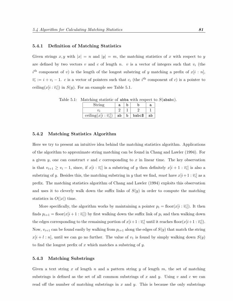
5.4 Algorithm for Calculating Matching Statistics 81
5.4.1 Definition of Matching Statistics
Given strings x, y with |x| = n and |y| = m, the matching statistics of x with respect to y
are defined by two vectors v and c of length n. v is a vector of integers such that vi (the
ith component of v) is the length of the longest substring of y matching a prefix of x[i : n],
vi := i + vi − 1. c is a vector of pointers such that ci (the ith component of c) is a pointer to
ceiling(x[i : vi]) in S(y). For an example see Table 5.1.
Table 5.1: Matching statistic of abba with respect to S(ababc).String a b b avi 2 1 2 1
ceiling(x[i : vi]) ab b babc$ ab
5.4.2 Matching Statistics Algorithm
Here we try to present an intuitive idea behind the matching statistics algorithm. Applications
of the algorithm to approximate string matching can be found in Chang and Lawler (1994). For
a given y, one can construct v and c corresponding to x in linear time. The key observation
is that vi+1 ≥ vi − 1, since, if x[i : vi] is a substring of y then definitely x[i + 1 : vi] is also a
substring of y. Besides this, the matching substring in y that we find, must have x[i+1 : vi] as a
prefix. The matching statistics algorithm of Chang and Lawler (1994) exploits this observation
and uses it to cleverly walk down the suffix links of S(y) in order to compute the matching
statistics in O(|x|) time.
More specifically, the algorithm works by maintaining a pointer pi = floor(x[i : vi]). It then
finds pi+1 = floor(x[i+ 1 : vi]) by first walking down the suffix link of pi and then walking down
the edges corresponding to the remaining portion of x[i+1 : vi] until it reaches floor(x[i+1 : vi]).
Now, vi+1 can be found easily by walking from pi+1 along the edges of S(y) that match the string
x[i + l : n], until we can go no further. The value of v1 is found by simply walking down S(y)
to find the longest prefix of x which matches a substring of y.
5.4.3 Matching Substrings
Given a text string x of length n and a pattern string y of length m, the set of matching
substrings is defined as the set of all common substrings of x and y. Using v and c we can
read off the number of matching substrings in x and y. This is because the only substrings

5.5 Our Algorithm for String Kernels 82
which occur in both x and y are those which are prefixes of x[i : vi] for some i. The number
of occurrences of a substring in y can be found by lvs(ceiling(w)) (cf. Section 5.3.1). The two
lemmas below formalize this.
Lemma 19 w is a substring of x iff there is an i such that w is a prefix of x[i : n]. The number
of occurrences of w in x can be calculated by finding all such i.
Proof The proof is elementary. If w is a substring of x then w = x[i : i + |w| − 1] for some i
and hence w is a prefix of x[i : n]. Conversely every substring of the string x[i : n] (for some i)
is a substring of x and hence w is also a substring of x. It is also clear that every occurrence
of w in x satisfies the above property and hence the number of occurrences of w in x can be
calculated by counting such i which satisfy the above property.
Lemma 20 The set of matching substrings of x and y is the set of all prefixes of x[i : vi].
Proof Let w be a substring of both x and y. By above lemma there is an i such that w is a
prefix of x[i : n]. Since, vi is the length of the maximal prefix of x[i : n] which is a substring in
y, it follows that vi ≥ |w|. Hence, w must be a prefix of x[i : vi].
5.5 Our Algorithm for String Kernels
In this section we present a fast implementation strategy for the string kernels that we introduced
in Section 5.2. We make use of suffix trees that we introduced in Section 5.3 and a modified
form of the the Matching Statistics algorithm that we introduced in Section 5.4.
5.5.1 Our Algorithm
A rather naive, O(|x|.|x′|) time, algorithm for enumerating the matching substrings of two strings
is rather easy to obtain. The dynamic programming approach outlined in Herbrich (2002) also
requires O(|x|.|x′|) time. In case the weights of various substrings are completely independent
of each other we must consider the weight contribution of each substring and cannot do better
than the naive algorithm and we require at least O(|x|.|x′|) time. In most practical applications

5.5 Our Algorithm for String Kernels 83
the weights on the substrings have some relation with each other and by exploiting this relation
we can compute the string kernel in linear time.
From the previous sections we know how to determine the set of all longest prefixes x[i : vi]
of x[i : n] in y in linear time. The following theorem uses this information to compute kernels
efficiently.
Theorem 21 Let x and y be strings and c and v be the matching statistics of x with respect
to y. Assume that floor(.), ceiling(.), father(.) and lvs(.) are computed on S(y). Furthermore
assume that
W (y, t) =
∑s∈prefix(z)
wus
− wu where u = floor(t) and t = uz. (5.2)
can be computed in constant time for any t. Then k(x, y) defined in Equation (5.1) can be
computed in O(|x|+ |y|) time as
k(x, y) =|x|∑i=1
val(x[i : vi]) =|x|∑i=1
(val(father(ci)) + lvs(ceiling(x[i : vi])) ·W (y, x[i : vi])
)(5.3)
where val(t) := lvs(ceiling(t)) ·W (y, t) + val(floor(t)) and val(root) := 0.
Proof We first show that Equation (5.3) can indeed be computed in linear time. We know that
for S(y) the number of leaves can be computed in linear time and likewise c, v. By assumption
on W (y, t) and by exploiting the recursive nature of val(t) we can compute W (y,nodes(i)) for
all the nodes of S(y) by a simple top down procedure in O(|y|) time.
Also, due to recursion, the second equality of Equation (5.3) holds and we may compute each
term in constant time by a simple lookup for val(father(ci)) and computation of W (y, x[i : vi]).
Since we have |x| terms, the whole procedure takes O(|x|) time, which proves the O(|x| + |y|)
time complexity.
Now, we prove that Equation (5.3) really computes the kernel. We know from Lemma 20
that the sum in Equation (5.1) can be decomposed into the sum over matches between y and
each of the prefixes of x[i : vi] (this takes care of all the substrings in x matching with y). This
reduces the problem to showing that each term in the sum of Equation (5.3) corresponds to the
contribution of all prefixes of x[i : vi].
Assume we descend down the path x[i : vi] in S(y) (e.g., for the string bab with respect

5.6 Weights and Kernels 84
to the tree of Figure 5.1 this would correspond to (root, b, bab)), then each of the prefixes t
along the path (e.g., (’’, b, ba, bab) for the example tree) occurs exactly as many times as
lvs(ceiling(t)) does. In particular, prefixes ending on the same edge occur the same number of
times. This allows us to bracket the sums efficiently, and W (y, x) simply is the sum along an
edge, starting from the floor of x to x. Unwrapping val(x) shows that this is simply the sum
over the occurrences on the path of x, which proves our claim.
Our algorithm works by a slight modification of the matching statistics algorithm and is illus-
trated in Algorithm 5.2. The algorithm takes as input an annotated suffix tree S(y). At the end
of line 18 we know that the longest matching prefix of x[i : n] which is a substring in y is x[i : k].
By Lemma 20 we know that the only possible matching substrings of x and y are the prefixes
of x[i : k] for i = 1, . . . , |x|. Each occurrence of the string x[i : l], where l ≤ k, contributes wx[i:l]
weight to the kernel. But, the number of occurrences of x[i : l] is simply lvs(ceiling(x[i : l]), so,
its total weight contribution is lvs(ceiling(x[i : l]))× wx[i:l]. By the annotation of nodes of S(y)
we know that val(v) denotes the total weight contribution due to x[i : j]. Now, the number of
occurrences of x[i : j + 1], x[i : j + 2] . . . x[i : k] is simply lvs(son(v, x(j + 1))) because they lie
on the same edge and hence share the same ceiling node. Therefore, the contribution due to
x[i : j + 1], x[i : j + 2], . . . , x[i : k] is given by W (y, x[i : k]) ∗ lvs(ceiling(x[i : k])). The algorithm
sums up the contribution due to x[i : j] in line 19 and the contribution due to x[j + 1 : k] in
line 21 and repeats this for all x[i : k], i = 1, . . . , |x|. Hence, by the definition of k(x, y) in
Equation (5.1), val = k(x, y) in line 32.
5.6 Weights and Kernels
So far, our claim hinges on the fact that W (y, t) can be computed in constant time, which is far
from obvious at first glance. We now show that this is a reasonable assumption in all practical
cases.
Length Dependent Weights If the weights ws depend only on |s| we have ws = w|s|. Define
ωj :=∑j
i=1wj and compute its values beforehand up to ωJ where J ≥ |x| for all x. Then it
follows that
W (y, t) =|t|∑
j=| floor(t)|
wj − w| floor(t)| = ω|t| − ω| floor(t)| (5.4)

5.6 Weights and Kernels 85
Algorithm 5.2: String Kernel Calculationinput x, y, S(y)output k(x, y)1: Let v ← root(S(y))2: Let j ← 13: Let k ← 14: Let val← 05: for i = 1 to |x| do6: while (j < k) and (j + len(v, x(j)) ≤ k) do7: v ← son(v, x(j))8: j ← j + len(v, x(j))9: end while
10: if (j = k) then11: while son(v, x(j)) exists and (x(k) = y(first(v, x(j)) + k − j)) do12: k ← k + 113: if (j + len(v, x(j)) = k) then14: v ← son(v, x(j))15: j ← k16: end if17: end while18: end if19: val← val + val(v)20: if (j < k) then21: val← val + lvs(ceiling(x[i : k])) ∗W (y, x[i : k])22: end if23: if v = root(S(y)) then24: j ← j + 125: if (j = k) then26: Let k ← k + 127: end if28: else29: v ← shift(v)30: end if31: end for32: return val
5.6 Weights and Kernels 86
which can be computed in constant time. Examples of such weighting schemes are the kernels
suggested by Watkins (2000), where wi = λ−i, Haussler (1999) where wi = 1, and Joachims
(1999), where wi = δ1i.
Generic Weights In case of generic weights, we have several options: recall that one often
will want to compute m2 kernels k(x, x′), given m strings x ∈ X . Hence, we could build the suffix
trees for xi beforehand and annotate each of the nodes and characters on the edges explicitly
(at super-linear cost per string), which means that later, for the dot products, we will only need
to perform table lookup of W (x, x′[i : vi]).
However, there is an even more efficient mechanism, which can even deal with dynamic
weights, depending on the relative frequency of occurrence of the substrings in X . We can build
the suffix tree S(X ) in time linear in the total length of all the strings. It can be shown that for
all x and all i, x[i : vi] will be a node in this tree (Vishwanathan and Smola, 2002). This implies
that it is sufficient to annotate each node of S(X ) with the value of W (.) in order to compute
each one of the m2 kernels. Since there are at most O(m) such nodes we need to perform only
O(m) annotations. Another advantage of this scheme is that leaves counting allows us to get
the number of occurrences of a substring in X . This information is extremely useful when we
want to assign weights to substrings based on their frequency of occurrence.
In case we make the reasonable assumption that ws = ρ(freq(s)) · φ(|s|), that is, ws is a
function of the length and frequency only. Now, note that all the strings ending on the same
edge in S(X ) have the same frequency of occurrence (cf. Section 5.3.2). Hence, we can rewrite
Equation (5.2) as
W (y, t) =
∑s∈prefix(z)
wus
− wu = ρ(freq(t))
|t|∑i=| floor(t)|+1
φ(i)
− wu (5.5)
where u = floor(t) and t = uz. By pre-computing∑
i φ(i) we can evaluate Equation (5.5) in
constant time. The benefit of Equation (5.5) is twofold: we can compute the weights of all the
nodes of S(X ) in time linear in the total length of strings in X . Secondly, for arbitrary x we can
compute W (y, t) in constant time, thus allowing us to compute k(xi, x′) in O(|xi|+ |x′|) time.

5.7 Linear Time Prediction 87
5.7 Linear Time Prediction
Let X s = {x1, x2, . . . , xm} be the set of Support Vectors. Recall that, for prediction in a Support
Vector Machine we need to compute
f(x) =m∑
i=1
αik(xi, x),
which implies that we need to combine the contribution due to matching substrings from each
one of the Support Vectors. We first construct S(X s) in linear time by using the Amir et al.
(1994) algorithm. In S(X s), we associate weight αi with each leaf associated with a Support
Vector xi. For a node v ∈ nodes(S(X s)) we modify the definition of lvs(v) as the sum of weights
associated with the subtree rooted at node v. Given the suffix tree S(y) the matching statistics of
a string x with respect to string y can be computed in O(|x|) time (cf. Section 5.4.2). Similarly,
given the suffix tree S(X s) we can find the matching statistics of string x with respect to all
strings in X s in O(|x|) time. Now, Algorithm 5.2 can be applied unchanged to compute f(x).
As is clear, our algorithm runs in time linear in the size of x and is independent of the size of
X s. To prove its correctness we use the following generalized definition of a matching substring.
Lemma 22 w is a matching substring of X s and x iff w v x and there exists a xi ∈ X s such
that w v xi.
We now extend Lemma 20 by incorporating the above definition
Lemma 23 The set of matching substrings of X s and x is the set of all prefixes of x[i : vi].
Proof Let w be a matching substring of X s and x. By Lemma 19 there is an i such that w is
a prefix of x[i : n]. Since, vi is the length of the maximal prefix of x[i : n] which is a substring
in some xj ∈ X s, it follows that vi ≥ |w|. Hence, w must be a prefix of x[i : vi].
The above lemma shows that we can apply Theorem 21 and use Algorithm 5.2 to compute f(x)
as long as we can bracket the weights efficiently. Rewriting f(x) using Equation (5.1)
f(x) =m∑
i=1
αi
∑svx,s′vy
wsδs,s′ =∑
svx,s′vy
p∑i=1
(αiws)δs,s′ , (5.6)

5.8 Tree Kernels 88
we notice that each occurrence of a substring s instead of contributing a weight ws now con-
tributes a weight of αiws, which is taken into account by the modified definition of lvs(v), hence,
proving the correctness of our algorithm.
In the case of SimpleSVM (cf. Chapter 2 ) the number of Support Vectors changes dynami-
cally i.e., Support Vectors are either added or deleted during each iteration. In such cases also
we can insert and delete Support Vectors from X s in time linear in the size of the Support
Vector string by using the Amir et al. (1994) algorithm and perform prediction in time linear in
the size of the string to classify.
5.8 Tree Kernels
We begin by introducing some notation. A tree is defined as a connected directed graph with no
cycles. A node with no children is referred to as a leaf. A subtree rooted at node n is denoted as
Tn. If a set of nodes in the tree along with the corresponding edges forms a tree then we define
it to be a subset tree. We use the notation T ′ |= T to indicate that T ′ is a subset tree of T . If
every node n of the tree contains a label, denoted by label(n), then the tree is called an labeled
tree. If only the leaf nodes contain labels then the tree is called a leaf-labeled tree. Kernels on
trees can be defined by defining kernels on matching subset trees. This is more general than
matching subtrees proposed in Collins and Duffy (2001). Here we have
k(T, T ′) =∑
t|=T,t′|=T ′
wtδt,t′ . (5.7)
That is, we count the number of occurrences of every subset tree t in both T and T ′ and weight
it by wt. Setting wt = 0 for all |t| > 1 yields the bag-of-nodes kernel, which simply counts
matching nodes. Setting ws = 0 for all subset trees that are not complete subtrees under some
node leads us to subtree kernels. They will be the main emphasis of this chapter.
5.8.1 Ordering Trees
An ordered tree is one in which the child nodes of every node are ordered as per the ordering
defined on the node labels. Unless there is a specific inherent order on the trees we are given
(which is, e.g., the case for parse-trees), the representation of trees is not unique. For instance,
the following two unlabeled trees are equivalent and can obtained from each other by reordering
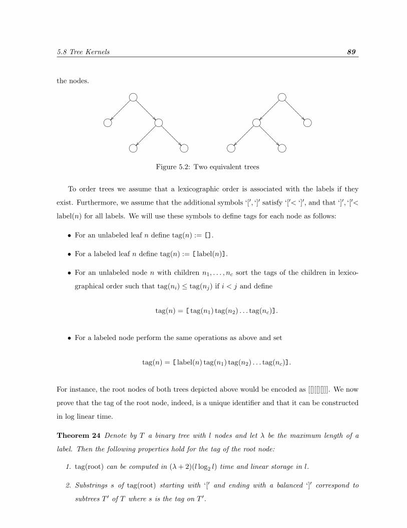
5.8 Tree Kernels 89
the nodes.
/.-,()*+
������
����
�
��???
????
??/.-,()*+
������
����
�
��???
????
??
/.-,()*+ /.-,()*+
������
����
�
��???
????
??/.-,()*+
������
����
�
��???
????
??/.-,()*+
/.-,()*+ /.-,()*+ /.-,()*+ /.-,()*+
Figure 5.2: Two equivalent trees
To order trees we assume that a lexicographic order is associated with the labels if they
exist. Furthermore, we assume that the additional symbols ‘[′, ‘]′ satisfy ‘[′< ‘]′, and that ‘]′, ‘[′<
label(n) for all labels. We will use these symbols to define tags for each node as follows:
• For an unlabeled leaf n define tag(n) := [].
• For a labeled leaf n define tag(n) := [ label(n)].
• For an unlabeled node n with children n1, . . . , nc sort the tags of the children in lexico-
graphical order such that tag(ni) ≤ tag(nj) if i < j and define
tag(n) = [ tag(n1) tag(n2) . . . tag(nc)].
• For a labeled node perform the same operations as above and set
tag(n) = [ label(n) tag(n1) tag(n2) . . . tag(nc)].
For instance, the root nodes of both trees depicted above would be encoded as [[][[][]]]. We now
prove that the tag of the root node, indeed, is a unique identifier and that it can be constructed
in log linear time.
Theorem 24 Denote by T a binary tree with l nodes and let λ be the maximum length of a
label. Then the following properties hold for the tag of the root node:
1. tag(root) can be computed in (λ+ 2)(l log2 l) time and linear storage in l.
2. Substrings s of tag(root) starting with ‘[′ and ending with a balanced ‘]′ correspond to
subtrees T ′ of T where s is the tag on T ′.
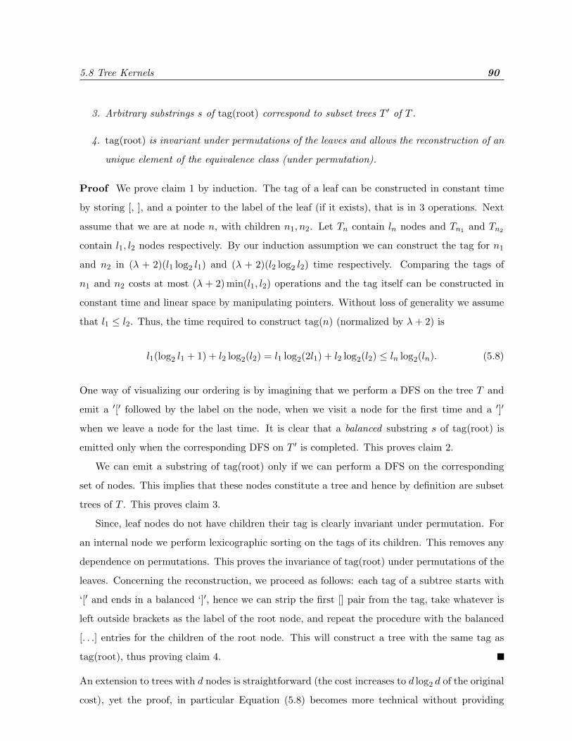
5.8 Tree Kernels 90
3. Arbitrary substrings s of tag(root) correspond to subset trees T ′ of T .
4. tag(root) is invariant under permutations of the leaves and allows the reconstruction of an
unique element of the equivalence class (under permutation).
Proof We prove claim 1 by induction. The tag of a leaf can be constructed in constant time
by storing [, ], and a pointer to the label of the leaf (if it exists), that is in 3 operations. Next
assume that we are at node n, with children n1, n2. Let Tn contain ln nodes and Tn1 and Tn2
contain l1, l2 nodes respectively. By our induction assumption we can construct the tag for n1
and n2 in (λ + 2)(l1 log2 l1) and (λ + 2)(l2 log2 l2) time respectively. Comparing the tags of
n1 and n2 costs at most (λ + 2)min(l1, l2) operations and the tag itself can be constructed in
constant time and linear space by manipulating pointers. Without loss of generality we assume
that l1 ≤ l2. Thus, the time required to construct tag(n) (normalized by λ+ 2) is
l1(log2 l1 + 1) + l2 log2(l2) = l1 log2(2l1) + l2 log2(l2) ≤ ln log2(ln). (5.8)
One way of visualizing our ordering is by imagining that we perform a DFS on the tree T and
emit a ′[′ followed by the label on the node, when we visit a node for the first time and a ′]′
when we leave a node for the last time. It is clear that a balanced substring s of tag(root) is
emitted only when the corresponding DFS on T ′ is completed. This proves claim 2.
We can emit a substring of tag(root) only if we can perform a DFS on the corresponding
set of nodes. This implies that these nodes constitute a tree and hence by definition are subset
trees of T . This proves claim 3.
Since, leaf nodes do not have children their tag is clearly invariant under permutation. For
an internal node we perform lexicographic sorting on the tags of its children. This removes any
dependence on permutations. This proves the invariance of tag(root) under permutations of the
leaves. Concerning the reconstruction, we proceed as follows: each tag of a subtree starts with
‘[′ and ends in a balanced ‘]′, hence we can strip the first [] pair from the tag, take whatever is
left outside brackets as the label of the root node, and repeat the procedure with the balanced
[. . .] entries for the children of the root node. This will construct a tree with the same tag as
tag(root), thus proving claim 4.
An extension to trees with d nodes is straightforward (the cost increases to d log2 d of the original
cost), yet the proof, in particular Equation (5.8) becomes more technical without providing

5.9 Experimental Results 91
additional insight, hence we omit this generalization for brevity.
Corollary 25 Kernels on trees T, T ′ can be computed via string kernels, if we use tag(T ), tag(T ′)
as strings. If we require that only balanced [. . .] substrings have nonzero weight ws then we obtain
the subtree matching kernel defined in Collins and Duffy (2001).
This reduces the problem of tree kernels to string kernels and as we have already seen string ker-
nels can be computed efficiently in linear time. Hence, the tree kernel k(T, T ′) can be computed
in O(l log(l)) time where l is the total number of nodes in T and T ′.
5.8.2 Coarsening
We now turn our attention to efficient evaluation of coarsening levels defined in Section 4.5.3.
It is clear that calculating the general tree kernel defined in Equation (4.10) is very difficult.
Instead we focus our attention on the kernel defined in Equation (4.11). Let ST represent a string
corresponding to an unlabeled tree T . To obtain ST1 we simply need to delete all occurrences
of [∗] where ∗ is a wildcard representing the label on a leaf node. By recursively applying this
procedure d times we can obtain STd. To calculate STd
from STd−1we require O(|STd−1
|) time.
Given two trees T and T ′ we can compute the kernel defined in Equation (4.11) by us-
ing Algorithm 5.3. The while loop requires O(min(|ST |, |ST ′ |)) for execution and it executes
O(min(|ST |, |ST ′ |)) times. Thus the whole algorithm now scales as quadratic in the size of the
trees. But, if we assume that during each deletion the length of ST and ST ′ reduce strictly by a
factor of λ < 1, then the algorithm is linear in the size of the trees and total work done by the
algorithm in this case is
∑i
(|ST |+ |ST ′ |)λi =1
1− λ(|ST |+ |ST ′ |). (5.9)
5.9 Experimental Results
The main point of this chapter is to introduce a novel means of evaluating string kernels efficiently
and to present theoretical guarantees on its time complexity. Hence, we do not concentrate our
efforts on presenting a wide variety of applications (separate papers focusing on applications
are currently under preparation). Here we present a proof of concept application for a remote

5.9 Experimental Results 92
Algorithm 5.3: Calculating kcoarse(T, T ′)input ST , ST ′
output kcoarse(T, T ′)1: Let val← 02: while ST 6= null and ST ′ 6= null do3: val← val +Wi × k(ST , ST ′)4: ST = delete(ST , [∗])5: ST ′ = delete(ST ′ , [∗])6: end while7: return val
homology detection problem from Jaakkola et al. (2000). Details of the experiments and data
sets are available at www.cse.ucsc.edu/research/compbio/discriminative. We use a length
weighted kernel and assign a weight λl for all matches of length greater than 3. We use a
publicly available SVM software implementation (www.cs.columbia.edu/compbio/svm), which
implements a soft margin optimization algorithm.
The ROC50 score is the area under the receiver operating characteristic curve (the plot of
true positives as a function of false positives) up to the first 50 false positives. A score of 1
indicates perfect separation of positives from negatives, whereas a score of 0 indicates that none
of the top 50 sequences selected by the algorithm were positives (Gribskov and Robinson, 1996).
Since this is a proof of concept implementation no parameter tuning of the soft margin SVM
was performed. We experimented with various values of λ ∈ {0.25, 0.5, 0.75, 0.9} and report
our best results for λ = 0.75 here. The ROC50 scores are compared with the spectrum kernel
algorithm of Leslie et al. (2002a) (they report best results for k = 3) in Figure 5.3. We also
observed that our kernel outperforms the spectrum kernel on nearly every every family in the
dataset and for all values of λ that we tested on.
It should be noted that this is the first method to allow users to specify weights rather
arbitrarily for all possible lengths of matching sequences and still be able to compute kernels
at O(|x|+ |x′|) time, plus, to predict on new sequences at O(|x|) time, once the set of Support
Vectors is established.

5.10 Summary 93
Figure 5.3: Total number of families for which a SVM classifier exceeds a ROC50 score threshold
5.10 Summary
We have shown that string kernels need not come at a super-linear cost and that prediction can
be carried out at cost linear only in the length of the argument, thus providing optimal run-time
behavior. Furthermore the same algorithm can be applied to trees as well.
We consider coarsening levels for trees by removing some of the leaves. For not too-
unbalanced trees (we assume that the tree shrinks at least by a constant factor at each coars-
ening) computation of the kernel over all coarsening levels can then be carried out at cost still
linear in the overall size of the tree. The coarsening ideas can be extended to approximate string
matching. If we remove characters, this amounts to the use of wildcards.
Likewise, we can consider the strings generated by finite state machines and thereby compare
the finite state machines themselves. This leads to kernels on Automata and other dynamical
systems. More details and extensions can be found in Chapter 4 as well as in Vishwanathan and
Smola (2002).
Applications of our string kernel to areas as diverse as spam filtering, network intrusion
detection, web search engines, document retrieval, bio-informatics and finite state transducers
are areas of active research.

Chapter 6
Kernels and Dynamic Systems
This chapter explores the relationship between dynamic systems and kernels. Kernels on various
kinds of dynamic systems including Markov chains (both discrete and continuous), diffusion
processes on graphs and Markov chains, Finite State Automata (FSA), various linear time-
invariant systems etc. are defined. Trajectories are used to define kernels induced on initial
conditions by the underlying dynamic system. The same idea is extended to define kernels on
a dynamic system with respect to a set of initial conditions. This framework leads to a large
number of novel kernels and also generalizes many previously proposed kernels.
In Section 6.1 we introduce and motivate the problem and present a generic model relating
kernels and dynamic systems. In Section 6.2 we review basic facts from control theory pertaining
to linear time-invariant systems (both discrete and continuous). In Section 6.3 we study kernels
defined using linear time-invariant systems and consider various special cases that arise out of our
model and their relation to previously proposed kernels. In Section 6.4 we study kernels defined
on linear time-invariant systems. We conclude with a discussion and summary in Section 6.5.
This chapter requires basic knowledge of kernels as discussed in Section 1.3. Knowledge
of elementary concepts from probability theory are assumed throughout the chapter(cf. Feller
(1950)). Section 6.2 reviews a few concepts from control theory related to linear time-invariant
systems. For a more complete review and detailed derivations see Luenberger (1979). Familiarity
with basic concepts from Markov chains, graphs, linear algebra and linear differential equations
is assumed throughout this chapter.
94
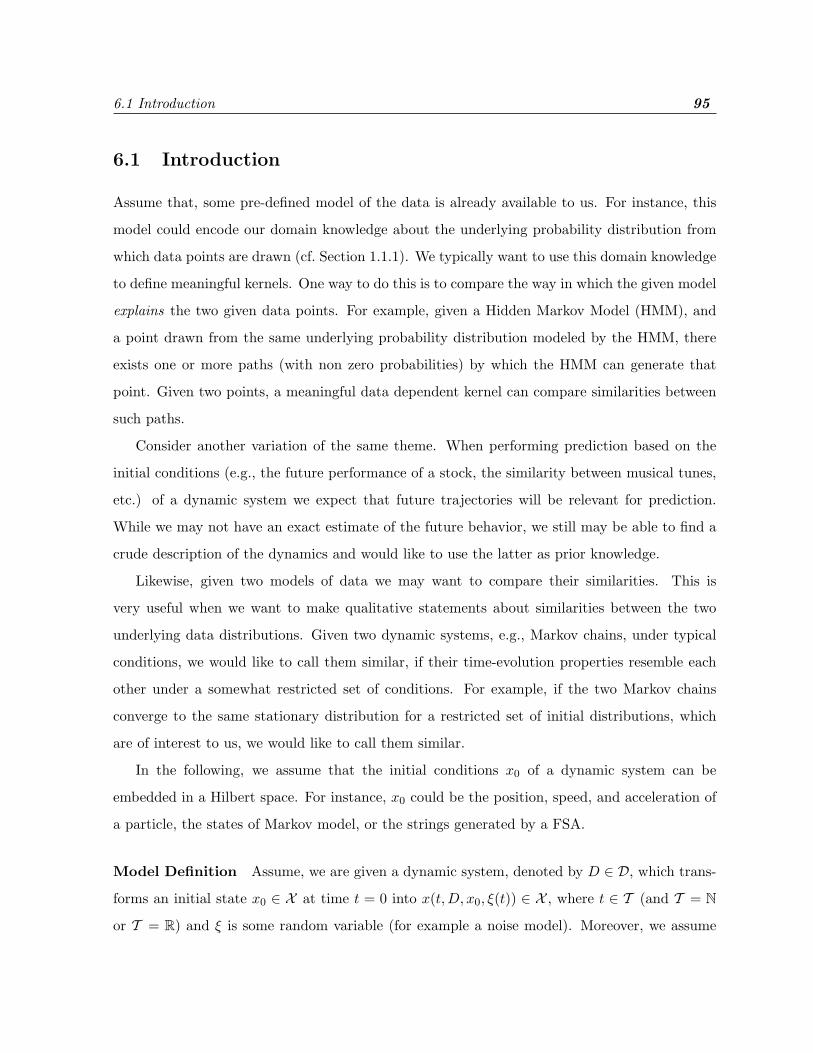
6.1 Introduction 95
6.1 Introduction
Assume that, some pre-defined model of the data is already available to us. For instance, this
model could encode our domain knowledge about the underlying probability distribution from
which data points are drawn (cf. Section 1.1.1). We typically want to use this domain knowledge
to define meaningful kernels. One way to do this is to compare the way in which the given model
explains the two given data points. For example, given a Hidden Markov Model (HMM), and
a point drawn from the same underlying probability distribution modeled by the HMM, there
exists one or more paths (with non zero probabilities) by which the HMM can generate that
point. Given two points, a meaningful data dependent kernel can compare similarities between
such paths.
Consider another variation of the same theme. When performing prediction based on the
initial conditions (e.g., the future performance of a stock, the similarity between musical tunes,
etc.) of a dynamic system we expect that future trajectories will be relevant for prediction.
While we may not have an exact estimate of the future behavior, we still may be able to find a
crude description of the dynamics and would like to use the latter as prior knowledge.
Likewise, given two models of data we may want to compare their similarities. This is
very useful when we want to make qualitative statements about similarities between the two
underlying data distributions. Given two dynamic systems, e.g., Markov chains, under typical
conditions, we would like to call them similar, if their time-evolution properties resemble each
other under a somewhat restricted set of conditions. For example, if the two Markov chains
converge to the same stationary distribution for a restricted set of initial distributions, which
are of interest to us, we would like to call them similar.
In the following, we assume that the initial conditions x0 of a dynamic system can be
embedded in a Hilbert space. For instance, x0 could be the position, speed, and acceleration of
a particle, the states of Markov model, or the strings generated by a FSA.
Model Definition Assume, we are given a dynamic system, denoted by D ∈ D, which trans-
forms an initial state x0 ∈ X at time t = 0 into x(t,D, x0, ξ(t)) ∈ X , where t ∈ T (and T = N
or T = R) and ξ is some random variable (for example a noise model). Moreover, we assume
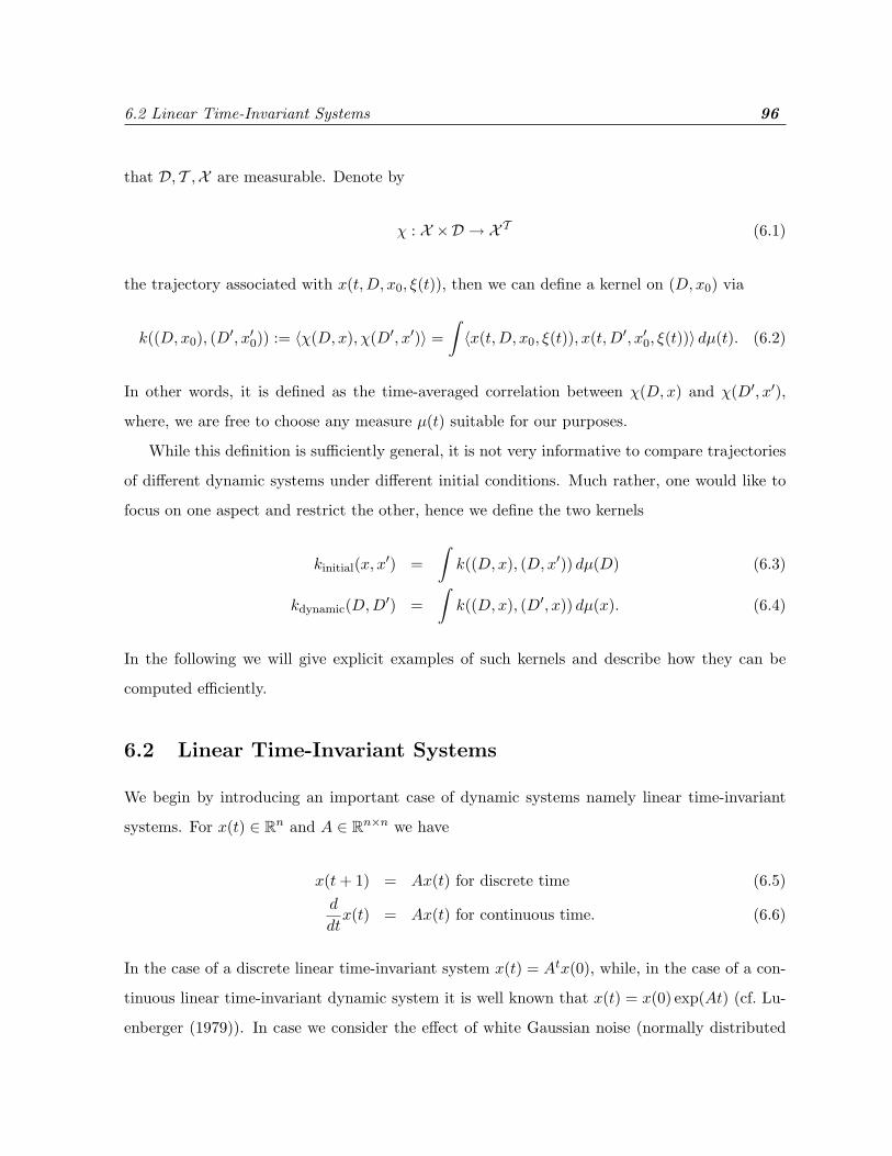
6.2 Linear Time-Invariant Systems 96
that D, T ,X are measurable. Denote by
χ : X ×D → X T (6.1)
the trajectory associated with x(t,D, x0, ξ(t)), then we can define a kernel on (D,x0) via
k((D,x0), (D′, x′0)) := 〈χ(D,x), χ(D′, x′)〉 =∫〈x(t,D, x0, ξ(t)), x(t,D′, x′0, ξ(t))〉 dµ(t). (6.2)
In other words, it is defined as the time-averaged correlation between χ(D,x) and χ(D′, x′),
where, we are free to choose any measure µ(t) suitable for our purposes.
While this definition is sufficiently general, it is not very informative to compare trajectories
of different dynamic systems under different initial conditions. Much rather, one would like to
focus on one aspect and restrict the other, hence we define the two kernels
kinitial(x, x′) =∫k((D,x), (D,x′)) dµ(D) (6.3)
kdynamic(D,D′) =∫k((D,x), (D′, x)) dµ(x). (6.4)
In the following we will give explicit examples of such kernels and describe how they can be
computed efficiently.
6.2 Linear Time-Invariant Systems
We begin by introducing an important case of dynamic systems namely linear time-invariant
systems. For x(t) ∈ Rn and A ∈ Rn×n we have
x(t+ 1) = Ax(t) for discrete time (6.5)d
dtx(t) = Ax(t) for continuous time. (6.6)
In the case of a discrete linear time-invariant system x(t) = Atx(0), while, in the case of a con-
tinuous linear time-invariant dynamic system it is well known that x(t) = x(0) exp(At) (cf. Lu-
enberger (1979)). In case we consider the effect of white Gaussian noise (normally distributed

6.3 Kernels On Initial Conditions 97
with zero mean and σ2 variance) we have
x(t+ 1) = Ax(t) + ξt for discrete time (6.7)d
dtx(t) = Ax(t) + ξt for continuous time. (6.8)
For the discrete case we can find x(t) by solving the above difference equation to obtain
x(t) = Atx(0) +t−1∑i=0
Aiξi. (6.9)
while in the continuous case x(t) is given by (cf. (Luenberger, 1979, Chapter2))
x(t) = x(0) exp(At) +∫ t
0exp(A(t− τ))ξ(τ) dτ. (6.10)
In the case of a non-homogeneous linear time-invariant system we have
x(t+ 1) = A(x(t) + a) + ξt, (6.11)
where, a is constant and, as before, ξ is zero mean white Gaussian noise with variance σ2. Here
we can find x(t) using (cf. (Luenberger, 1979, Chapter2))
x(t) = Atxa + a+t−1∑i=0
Aiξi, (6.12)
where,
a := (1−A)−1a, (6.13)
and
xa := x(0)− (1−A)−1a = x(0)− a. (6.14)
6.3 Kernels On Initial Conditions
Often, the transformations applied to the data, prior to computing dot products, can only
be specified implicitly by specifying the algorithm which will carry out the transformations.
For instance, we might consider all the transformations that a Non-Deterministic Finite State

6.3 Kernels On Initial Conditions 98
Automata (NFA) might apply to a string and consider the resulting set of possible outcomes as
the set of features to compute a dot product with. Likewise, we could consider a Markov model
and study the evolution of the states over time, thereby comparing the similarity between various
states. Finally, we could study a diffusion process on a (directed) graph and infer similarities.
6.3.1 Discrete Time Systems
We can define kernels on discrete linear time-invariant systems using Equation (6.5) and Equa-
tion (6.3) to get
k(x, x′) =∞∑
t=0
ct(Atx)>W (Atx′) = x>
[ ∞∑t=0
ct(At)>WAt
]x′. (6.15)
Here ct’s are arbitrary weights and W ∈ Rn×n is a covariance matrix. In general, Equation (6.15)
will be difficult to compute in closed form and may not be well defined for most assignments of
ct. For specific types of ct, however, such an expression can be found efficiently. The following
lemma, which we state in a somewhat more general form, gives an expansion for ct = λt for a
specific range of values of λ.
Lemma 26 Let ‖A‖ denote the 2-norm of A ∈ Rn×n. Let A,B,W ∈ Rn×n be such that the
singular values of A and B be bounded by Λ, i.e., ‖A‖, ‖B‖ ≤ Λ. Then, for all |λ| < 1Λ2 the
series
M :=∞∑
t=0
λt(At)>W (Bt) (6.16)
converges and M can be computed by solving λA>MB +W = M .
Proof To show that M is well defined we use the triangular inequality, leading to
‖M‖ =
∥∥∥∥∥∞∑
t=0
λt(At)>W (Bt)
∥∥∥∥∥ ≤∞∑
t=0
∥∥∥λt(At)>W (Bt)∥∥∥ ≤ ∞∑
t=0
(|λ|Λ2
)t ‖W‖ =‖W‖
1− |λ|Λ2.
Next, we decompose M into the first term of the sum and the remainder to obtain
M = λ0(A0)>WB0 +∞∑
t=1
λt(At)>W (Bt) = W + λA>
[ ∞∑t=0
λt(At)>W (Bt)
]B = W + λA>MB.
This concludes our proof.

6.3 Kernels On Initial Conditions 99
Corollary 27 The kernel k(x, x′), as defined in Equation (6.15) with ct = λt can be computed
as
k(x, x′) = x>Mx where λA>MA+W = M. (6.17)
Furthermore, for ct = δt,T we have the somewhat trivial kernel
k(x, x′) = x>(AT )>WATx. (6.18)
Note that Sylvester equations of type
AXB> + CXD> = E, (6.19)
where, A,B,C,D ∈ Rn×n have been widely studied in control theory. Many software packages
exist for solving them in O(n3) time (Gardiner et al., 1992, Hopkins, 2002).
We now extend our model to linear time-invariant systems with zero mean white Gaussian
noise and define the kernel as
k(x, x′) = Eξ
∞∑t=0
ct
(Atx+
t−1∑i=0
Aiξi
)>W
(Atx′ +
t−1∑i=0
Aiξi
)(6.20)
The expectation with respect to the random variable ξ means that we are considering the whole
ensemble of trajectories arising due to a certain noise model for given values of x and x′. As
before, the kernel can be computed in closed form for ct = λt, for certain values of λ (given by
Lemma 26). Since ξ is Gaussian white noise, and, x and all ξi are mutually independent we can
compute the contribution of ξi to the kernel independently. We first prove an auxiliary result.
Lemma 28 Let y ∈ Rn be a random vector such that C := E(yy>). Then, E(y>Wy) = tr (WC)
for all W ∈ Rn×n.
Proof Since, y>Wy is a scalar, expectation and trace commute since they are both linear
operators and tr (AB) = tr (BA) we can write
E(y>Wy) = E(tr (y>Wy)) = E(tr (W (yy>))) = tr (WE(yy>)) = tr (WC).
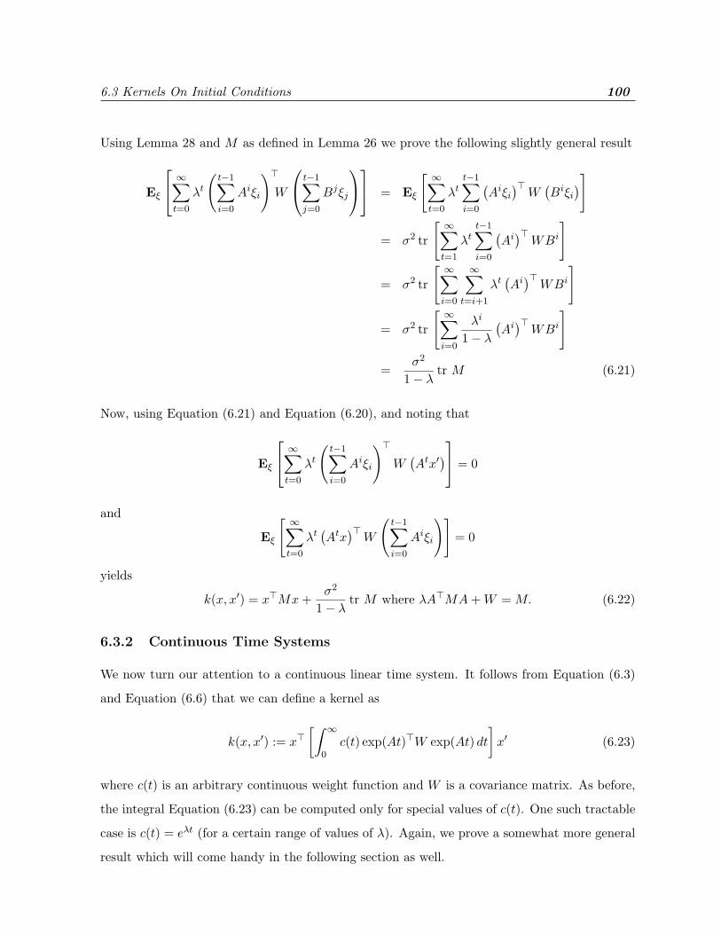
6.3 Kernels On Initial Conditions 100
Using Lemma 28 and M as defined in Lemma 26 we prove the following slightly general result
Eξ
∞∑t=0
λt
(t−1∑i=0
Aiξi
)>W
t−1∑j=0
Bjξj
= Eξ
[ ∞∑t=0
λtt−1∑i=0
(Aiξi
)>W(Biξi
)]
= σ2 tr
[ ∞∑t=1
λtt−1∑i=0
(Ai)>WBi
]
= σ2 tr
[ ∞∑i=0
∞∑t=i+1
λt(Ai)>WBi
]
= σ2 tr
[ ∞∑i=0
λi
1− λ(Ai)>WBi
]
=σ2
1− λtr M (6.21)
Now, using Equation (6.21) and Equation (6.20), and noting that
Eξ
∞∑t=0
λt
(t−1∑i=0
Aiξi
)>W(Atx′
) = 0
and
Eξ
[ ∞∑t=0
λt(Atx
)>W
(t−1∑i=0
Aiξi
)]= 0
yields
k(x, x′) = x>Mx+σ2
1− λtr M where λA>MA+W = M. (6.22)
6.3.2 Continuous Time Systems
We now turn our attention to a continuous linear time system. It follows from Equation (6.3)
and Equation (6.6) that we can define a kernel as
k(x, x′) := x>[∫ ∞
0c(t) exp(At)>W exp(At) dt
]x′ (6.23)
where c(t) is an arbitrary continuous weight function and W is a covariance matrix. As before,
the integral Equation (6.23) can be computed only for special values of c(t). One such tractable
case is c(t) = eλt (for a certain range of values of λ). Again, we prove a somewhat more general
result which will come handy in the following section as well.

6.3 Kernels On Initial Conditions 101
Lemma 29 Denote by A,B,W ∈ Rn×n such that ‖A‖, ‖B‖ ≤ Λ. Then, for all λ < −2Λ the
integral
M :=∫ ∞
0eλt exp(At)>W exp(Bt) dt (6.24)
converges and M is the solution of the Sylvester equation (A> + λ2 1)M +M(B + λ
2 1) = −W .
Proof Convergence of the integral is established via the triangular inequality, that is
‖M‖ ≤∫ ∞
0eλt‖ exp(At)>W exp(Bt)‖ dt ≤
∫ ∞
0exp((λ+ 2Λ)t)‖W‖ dt <∞. (6.25)
Furthermore, we have
M =∫ ∞
0etλetA
>WetB dt (6.26)
= (A>)−1etλetA>WetB
∣∣∣∞0−∫ ∞
0(A>)−1etλetA
>WetB(B + 1λ) dt (6.27)
= −(A>)−1W − (A>)−1M(B + λ1). (6.28)
Here we obtained Equation (6.27) by partial integration and Equation (6.28) by realizing that
the integrand vanishes for t → ∞ (for suitable λ) in order to make the integral convergent.
Multiplication by A> shows that M satisfies
A>M +MB + λM = −W. (6.29)
Rearranging terms and the fact that multiples of the identity matrix commute with A,B proves
the claim.
Corollary 30 The kernel k(x, x′), as defined in Equation (6.23) with c(t) = eλt can be computed
as
k(x, x′) = x>Mx where(A+
λ
21)>
M +M
(A+
λ
21)
= −W. (6.30)
Furthermore, for c(t) = δT (t) we have the somewhat trivial kernel
k(x, x′) = x>[exp(AT )>W exp(AT )
]x. (6.31)

6.3 Kernels On Initial Conditions 102
As before, we extend our model to linear time-invariant systems with zero mean white
Gaussian noise. Using Equation (6.10) we define the kernel as
k(x, x′) = Eξ
[∫ ∞
0c(t)P>WQdt
](6.32)
where, P := exp(At)x+∫ t0 exp(A(t− τ))ξ(τ) dτ and Q := exp(At)x′ +
∫ t0 exp(A(t− τ))ξ(τ) dτ .
We can compute the kernel in closed form for c(t) = exp(λt) (for certain values of λ given by
Lemma 29). Since, ξ is Gaussian white noise, and, x and ξ are mutually independent we can
compute the contribution of ξ to the kernel independently. Using Lemma 28 and M as defined
in Lemma 29 we prove the following slightly general result
Eξ
[∫ ∞
0exp(λt)
(∫ t
0exp(A(t− τ))ξ(τ) dτ
)>W
(∫ t
0exp(B(t− τ))ξ(τ) dτ
)dt
]
= Eξ
[∫ ∞
0exp(λt)
∫ t
0(exp(A(t− τ))ξ(τ))>W exp(B(t− τ))ξ(τ) dτ dt
]= σ2 tr
[−∫ ∞
0exp(λt)
∫ t
0exp(Ap)>W exp(Bp) dp dt
]= σ2 tr
[−∫ ∞
0
[∫ ∞
pexp(λt) exp(Ap)>W exp(Bp) dt
]dp
]=
σ2
λtr[∫ ∞
0exp(λp) exp(Ap)>W exp(Bp) dp
](6.33)
=σ2
λtr M. (6.34)
Here we obtained Equation (6.33) by noting that exp(λt)→ 0 as t→∞ (for values of λ defined
by Lemma 29). Now, using Equation (6.34) and Equation (6.32), and noting that
Eξ
[∫ ∞
0exp(λt)
(∫ t
0exp(A(t− τ))ξ(τ) dτ
)>W (exp(At)x′) dt
]= 0
and
Eξ
[∫ ∞
0exp(λt)(exp(At)x)>W
(∫ t
0exp(A(t− τ))ξ(τ) dτ
)dt
]= 0
yields
k(x, x′) = x>Mx+σ2
λtr M where
(A+
λ
21)>
M +M
(A+
λ
21)
= −W. (6.35)

6.3 Kernels On Initial Conditions 103
6.3.3 Special Cases
The kernels described above, appear somewhat simple minded at first sight. After all, we are
only replacing the standard Euclidean metric by the covariance of two trajectories under a
dynamic system. Below, we show how specific instances of such kernels can lead to many new
and interesting kernels.
Discrete Time Markov Chain: In a homogeneous Discrete Time Markov Chain (DTMC),
x(t) corresponds to the state at time t and the matrix A is the matrix of state transition
probabilities, i.e., Aij = p(i|j), which is the probability of arriving in state i when originating
from state j. This means that via the function k(., .) we can compute the overlap between states,
when originating from x = ei and x′ = ej . Finally, since A is a stochastic matrix (positive entries
with row-sum 1), its eigenvalues are bounded by 1 and therefore, any discounting factor λ < 1
will lead to a well-defined kernel.
Note that if 1/λ is much smaller than the mixing time, k will mostly measure the overlap
between the initial states x, x′ and the transient distribution on the DTMC (The stationary
distribution may also play a role, albeit a reduced one, in determining the final kernel). The
quantity of interest here will be the ratio between λ and the gap between 1 and the second
largest eigenvalue of A (Graham, 1999).
In other words, we are comparing the trajectories of two (discrete time) random walks on a
Markov chain. Choosing ci = δi,T , on the other hand, means that we compare a snapshot of the
distribution over states after exactly T time steps.
Continuous Time Markov Chain: In a homogeneous Continuous Time Markov Chain
(CTMC), x(t) corresponds to the state at time t and the matrix A (also called the rate matrix)
denotes the differential change in the concentration of states. When the CTMC reaches a state,
it stays there for an exponentially distributed random time (called the state holding time) with
a mean that depends only on the state. Now, we can define kernels using diffusion on CTMC’s
by plugging in the rate matrix A into Equation 6.30.
Diffusion on Graphs: A special case of diffusion on a CTMC is diffusion on a directed graph.
Here diffusion through each of the edges of the graph is constant (in the direction of the edge).
This means that, given a matrix representation of a graph via D (here Dij = 1 if an edge from

6.4 Kernels on Dynamic Systems 104
j to i exists), we compute the Laplacian L = D − diag(D 1) of the graph, and use the latter to
define the diffusion process ddtx(t) = Lx(t). Note that in the special case of W = 1, the entry
Mij for M = exp(Lt)> exp(Lt) tells us the probability that any other state l could have been
reached jointly from i and j (Kondor and Lafferty, 2002).
Undirected Graphs and Groups: Kondor and Lafferty (2002) suggested to study diffusion
on undirected graphs with W = 1. Their derivations are a special case of Equation (6.31). Note
that for undirected graphs the matrices D and L are symmetric. This has the advantage that
Equation (6.31) can be further simplified to
k(x, x′) = x> exp(LT )>W exp(LT )x = x> exp(2LT )x. (6.36)
Finally, if we study an even more particular example of a graph, namely the Cayley graph of
a group, we thereby have a means of imposing a kernel on the elements of a group (see also
Kondor and Lafferty (2002) for further details).
Differential Equations It is well known that any linear differential equation can be trans-
formed into a first order linear differential equation by including the state space (Hirsch and
Smale, 1974). This means that differential equations thereby impose a kernel on the initial
conditions. Similarity here corresponds to correlation of the state space trajectories.
6.4 Kernels on Dynamic Systems
We now extend the notion of a kernel to dynamic systems. This includes differential equations,
FSA, Markov chain, etc. A natural way of comparing the similarity between two systems,
D ∈ D and D′ ∈ D is to compare the trajectories χ(D,x(0)) and χ(D′, x(0)), given the same
starting values x(0). In other words, we will say that two systems D and D′ are close if their
time evolution is close for a restricted set of inputs. This closely resembles the idea of system
identification in the “Behavioral Framework”, as invented by Willems (1986a,b, 1987) (see also
(Weyer, 1992) for further details).
In the most general setting, we will consider a mapping of a set of initial sequences x(0) into

6.4 Kernels on Dynamic Systems 105
their full time trajectory and define a dot product on them. This leads to a kernel of the form
k(D,D′) := EξEx(0)kχ(χ(D,x(0)), χ(D′, x(0))). (6.37)
Here kχ is a kernel determining how the similarity between the trajectories is measured. The
expectation with respect to x(0) allows us to encode knowledge about the set of initial conditions
we are most interested in. For instance, two models may behave identically on all situations
of interest to the user, hence we should consider them identical, even though they may exhibit
completely different behavior in a set of initial conditions which never occurs in practice. The
expectation with respect to the random variable ξ means that we are considering the whole
ensemble of trajectories arising due to a certain noise model for a given value of x(0).
In the following we will give examples of such kernels. They are useful in two regards: firstly
they allow us to define a Hilbert space embedding of dynamic systems in order to estimate some
of their properties directly. Secondly, they allow us to define notions of proximity between two
dynamic systems.
6.4.1 Discrete Time Systems
Let A and B define two discrete linear time-invariant systems without noise. For the sake of
analytic tractability we use
kχ(χ(A, x(0)), χ(B, x(0))) = x(0)>[ ∞∑
t=0
ct(At)>WBt
]x(0) (6.38)
where, as before, ct denote arbitrary weights. Hence, Equation (6.37) can be used to define the
following kernel
k(A,B) = Ex(0)
[x(0)>
[ ∞∑t=0
λt(At)>WBt
]x(0)
]. (6.39)
If we consider a weighting scheme of the form ci = λi, then, we know from Lemma 26 that kχ is
well defined only for certain values of λ. For such values of λ we can evaluate the above kernel
as (cf. Lemma 26)
k(A,B) = Ex(0)x(0)>Mx(0) where M = W + λA>MB. (6.40)

6.4 Kernels on Dynamic Systems 106
As before, M can be computed in O(n3) time by solving the Sylvester equation. Let C :=
Ex(0)x(0)x(0)> be the covariance matrix of the random variable x(0). Then, we can simplify
Equation (6.40) using Lemma 28 as
k(A,B) = Ex(0)(x(0)>Mx(0)) = tr (MC). (6.41)
If we consider the effect of white Gaussian noise the kernel can be defined as
kχ(χ(A, x(0)), χ(B, x(0)))
= EξEx(0)
∞∑t=0
ct
(Atx(0) +
t−1∑i=0
Aiξi
)>W
(Btx(0) +
t−1∑i=0
Biξi
) (6.42)
As before, Equation (6.42) can be computed in closed form for ct = λt, for certain values
of λ (given by Lemma 26). Since ξ is Gaussian white noise, and, x and all ξi are mutually
independent we can compute the contribution of ξi to the kernel independently. Using Lemma 28,
Equation (6.21) and Equation (6.42), and noting that
EξEx(0)
∞∑t=0
λt
(t−1∑i=0
Aiξi
)>W(Btx(0)
) = 0
and
EξEx(0)
[ ∞∑t=0
λt(Atx(0)
)>W
(t−1∑i=0
Biξi
)]= 0
yields
k(x, x′) = tr (MC) +σ2
1− λtr M where M = W + λA>MB. (6.43)
6.4.2 Continuous Time Systems
Let A and B define two continuous linear time-invariant systems without noise. For the sake of
analytic tractability we use
kχ(χ(A, x(0)), χ(B, x(0))) = x(0)>[∫ ∞
0c(t) exp(At)>W exp(Bt) dt
]x(0) (6.44)

6.4 Kernels on Dynamic Systems 107
where, as before, c(t) is a continuous weighting function. Hence, Equation (6.37) and Equa-
tion 6.44 can be used to define the following kernel
k(A,B) := Ex(0)
[x(0)>
(∫ ∞
0c(t) exp(At)>W exp(Bt)dt
)x(0)
]. (6.45)
If we consider a weighting scheme of the form ct = etλ, then, we know from Lemma 29 that kχ
is well defined only for certain values of λ. For such values of λ we can evaluate the above kernel
as (cf. Lemma 29)
k(A,B) = Ex(0)x(0)>Mx(0) where(A+
λ
21)>
M +M
(B +
λ
21)
= −W. (6.46)
By a similar reasoning as above we can compute Equation (6.45) by evaluating
k(A,B) = tr (MC) (6.47)
where, C is the covariance matrix of x(0).
We extend our model to linear time-invariant systems with zero mean white Gaussian noise
and define the kernel as
k(x, x′) = EξEx(0)
[∫ ∞
0c(t)P>WQdt
](6.48)
where, P := exp(At)x(0) +∫ t0 exp(A(t − τ))ξ(τ) dτ and Q := exp(Bt)x(0) +
∫ t0 exp(B(t −
τ))ξ(τ) dτ . We can compute the kernel in closed form for c(t) = exp(λt) (for certain values
of λ given by Lemma 29). Since, ξ is Gaussian white noise, and, x and ξ are mutually in-
dependent we compute the contribution of ξi to the kernel independently. Using Lemma 28,
Equation (6.34) and Equation (6.48), and noting that
EξEx(0)
[∫ ∞
0exp(λt)
(∫ t
0exp(A(t− τ))ξ(τ) dτ
)>W (exp(Bt)x(0)) dt
]= 0
and
EξEx(0)
[∫ ∞
0exp(λt)(exp(At)x(0))>W
(∫ t
0exp(A(t− τ))ξ(τ) dτ
)dt
]= 0
6.4 Kernels on Dynamic Systems 108
yields
k(x, x′) = tr (MC) +σ2
λtr M where
(A+
λ
21)>
M +M
(A+
λ
21)
= −W. (6.49)
6.4.3 Non-Homogeneous Linear Time-Invariant Systems
In the case of non-homogeneous linear time-invariant systems we define a kernel using Equa-
tion (6.12) and Equation (6.37) as
k((A, a), (B, b)) = EξEx(0)
[x(0)>
( ∞∑t=0
λtP>WQ
)x(0)
]
where, P := Atxa + a+∑t−1
i=0 Aiξi and Q := Btxa + b+
∑t−1i=0 B
iξi
Since x(0) and all ξi are mutually independent and ξ is Gaussian white noise we can compute
the contributions of ξi and x to the kernel independently. We first compute the contribution
due to Atxa + a.
∞∑t=0
λt(Atxa + a)>W (Btxb + b)
= x>a Mxb + x>a (1− λA>)−1Wb+ a>W (1− λB)−1xb +1
1− λa>Wb. (6.50)
Next, we assume that x(0) has variance Ξ and mean µ0. Using Equation (6.14) we get
Ex(0)
[xax
>b
]= Ex(0)
[(x(0)− a)(x(0)− b)>
]= Ξ + (µ0 − a)(µ0 − b)>. (6.51)
Putting everything together, i.e., taking expectations with respect to x(0) and plugging in
Equation (6.50), Equation (6.21) and Equation (6.51) into Equation (6.50) yields:
k((A, a), (B, b))
= tr (MΞ) +σ2
1− λtr (M) + tr ((µ0 − a)>M(µ0 − b)) (6.52)
+(µ0 − a)>(1− λA>)−1Wb+ a>W (1− λB)−1(µ0 − b) +1
1− λa>Wb.
Clearly, λ has to be chosen so that it satisfies the conditions defined in Lemma 29, since otherwise
the kernel k((A, a), (b, a)) would not be defined, due to lack of existence of the solution of the

6.5 Summary 109
Sylvester matrix equation.
6.5 Summary
We proposed a framework to connect kernels and dynamic systems. We showed how special-
izations of this framework lead to kernels on initial systems with respect to a given dynamic
system and on a dynamic system with respect to a given set of initial conditions. We studied
the framework for linear time-invariant systems and showed that their specializations lead to
many new kernels. Our framework also generalizes many previously proposed kernels.
Chapter 7
Jigsawing: A Method to Create
Virtual Examples
This chapter describes a new method to generate virtual training samples in the case of hand-
written digit data. It uses the two dimensional suffix tree representation of a set of matrices to
encode an exponential number of virtual samples in linear space thus leading to an increase in
classification accuracy. A new kernel for images is proposed and an algorithm for computing it
in quadratic time is described. Methods to reduce the prediction time to quadratic in the size of
the test image by using techniques similar to those used for string kernels (cf. Section 5.7) are
also described. We conjecture that the time complexity can be further reduced by intelligently
using the suffix tree on matrices.
In Section 7.1 we introduce our notation and motivate the problem. In Section 7.2 we survey
algorithms for generating virtual examples and examine their relation to our method. A high
level description of our algorithm follows in Section 7.3. A detailed description of jigsawing along
with intuitive arguments to show why it works can be found in Section 7.4. We discuss some
novel applications in Section 7.5. We propose a new kernel on images in Section 7.6 and show
how it can be computed in quadratic time by using suffix trees on matrices. We also describe a
quadratic time prediction algorithm for Support Vector Machines in Section 7.6. We conclude
with a summary in Section 7.7.
This chapter requires basic knowledge of statistical learning theory as discussed in Chapter 1
(cf. Section 1.1). An understanding of suffix trees on strings and their generalization to matrices
is essential. Readers may want to review Section 5.3 and the influential papers by Giancarlo
110

7.1 Background and Notation 111
(1995) and Cole and Hariharan (2000). Kim and Park (1999) also propose an alternate lin-
ear time construction algorithm for suffix trees on matrices. A review of convolution kernels
discussed in Section 4.2 and tree kernels discussed in Sections 4.5 and 5.8 maybe helpful in
understanding parts of this chapter.
7.1 Background and Notation
It is well known that the empirical risk of a classifier can be reduced by training it on a large
number of samples (Duda et al., 2001, Vapnik, 1995). In many real life situations the dataset
size may be limited or it may be expensive to obtain new samples for training (Niyogi et al.,
1998). But, we usually have some prior domain knowledge about the data which can be used
to generate virtual training samples. Some successful attempts in this direction especially for
handwritten digit datasets include methods like bootstrapping (Hamamoto et al., 1997) and
Partitioned Pattern Classification (PPC) trees (Viswanath and Murty, 2002). The methods
proposed by Niyogi et al. (1998) are applicable for object recognition and speech recognition.
In this chapter, we propose a novel method to generate exponential number of virtual training
samples by encoding the handwritten digit data in a two dimensional suffix tree using linear
space and linear construction time.
In the following, we denote by X = {(x1, y1), . . . , (xn, yn)} ⊂ Σ2k×2k × C the set of labeled
training samples1, where, C is the set of class labels, Σ is a finite ordered alphabet and we define
m := 2k. Without loss of generality we assume that $ /∈ Σ is a special symbol, ∗ ∈ Σ is a blank
character and C = {1, 2, . . . , c}. Furthermore, for i ∈ C, let X i denote the data points in class i
and let ni = | X i |. Let F (X i) denote a representation of X i, for example, it could be an array
that stores X i. A sample (x, i) is said to be virtual if it can be generated from F (X i). It is
clear that the only virtual samples generated by the array representation are (xj , i) such that
xj ∈ X i, while, other representations may yield a richer set of virtual samples. At this point, it
must be noted that, all the virtual training samples generated may not be meaningful, in fact,
many of them may be noisy patterns or outliers. Our ultimate goal is to use domain knowledge
to generate as many meaningful virtual samples as possible.
The suffix tree is a compacted trie that stores all suffixes of a given text string (Weiner,
1The assumption xi ∈ Σ2k×2k
looks very restrictive, but, is required mainly for notational convenience. Oneway to overcome this is to pad the data with sufficient number of blanks.
7.2 Related Work 112
1973, McCreight, 1976). It has been widely used for compact representation of input text and
in a wide variety of search applications (Grossi and Italiano, 1993) (cf. Section 5.3). Giancarlo
(1995) generalized the notion of a suffix tree on a string to suffix trees on arbitrary matrices
(also see Giancarlo and Grossi (1996, 1997), Giancarlo and Guaiana (1999)). We denote the
suffix tree of a matrix x by S(x). For each square sub-matrix of x, there is a corresponding path
in the suffix tree S(x). Linear time and linear space (that is O(m2)) algorithms for constructing
such suffix trees have recently been proposed by Cole and Hariharan (2000) (see Kim and Park
(1999) for an alternate algorithm).
Let nodes(S(x)) denote the set of all nodes of S(x) and root(S(x)) be the root of S(x).
For a node w, T (w) denotes the subtree tree rooted at the node, lvs(w) denotes the number
of leaves in the subtree. We denote by words(S(x)) the set of all sub-matrices of x. For every
t ∈ words(S(x)) we define ceiling(t) and floor(t) exactly analogous to their definitions on suffix
trees for strings (cf. Section 5.3.1).
The suffix tree of the set X i, denoted by S(X i), can be built in O(m2ni) time by merging
S(xj) for all (xj , i) ∈ X i. Giancarlo (1995) showed that all occurrences in X i of y ∈ Σp×p for
some p ≤ m can be found in O(p2) time. We use the notation y v X i to denote that y occurs
as a sub-matrix of some element of X i.
7.2 Related Work
Let D be the domain from which samples are drawn and T : Dt → D be a transformation which
maps a set of t training samples into a new meaningful sample. Virtual training samples can be
generated by applying the transformation T to the elements of the training set (Niyogi et al.,
1998). Different methods differ in the way they select the transformation function T and the
value of t.
Bootstrapping is a robust and well studied method to generate virtual samples from limited
training data (see for example Efron and Tibshirani, 1994, Efron, 1982). Variants of boot-
strapping have been successfully used for a wide variety of pattern recognition tasks (Efron
and Tibshirani, 1997, Kohavi, 1995). The basic idea behind bootstrapping is to generate new
samples by combining a set of closely related samples. For example, one method is to replace
a set of spatially close points by their centroid or their medoid (Hamamoto et al., 1997). The
main advantage of bootstrapping is that it is robust and well studied. But, it requires explicit

7.3 Basic Idea 113
storage of the generated samples and hence its use is generally constrained by memory and
storage considerations.
A trie is a multi-way tree structure used for storing strings over an alphabet (Fredkin, 1960).
Viswanath and Murty (2002) proposed the PPC tree which partitions the dataset vertically into
blocks and constructs a separate trie for each block. They show that the PPC tree can generate
virtual samples implicitly by combining data from various blocks. The advantage of the PPC
tree is that it uses linear space to encode a large number of virtual samples. But, the main
disadvantage is that the partitioning into blocks is highly dataset dependent (Viswanath and
Murty, 2002). Besides, it does not generalize well to take into consideration the two dimensional
nature of handwritten digit data. In handwritten digit datasets, the structure of the data plays
an important role in classification algorithms and hence a method which takes into account the
connected regions of a training sample is preferable. As of now, the PPC tree has been used
only with a k -Nearest Neighbor Classifier.
An immediately apparent application of the suffix tree on matrices is to search for all oc-
currences of a test pattern in the training set (Giancarlo, 1995). In real world applications, the
probability of finding an exact match between training samples and a test sample is negligible.
Hence, such a scheme is not practically feasible as a classification algorithm. It is clear that
we need to allow some kind of approximate matches in order to tackle this problem. Besides,
this scheme does not produce any virtual examples and hence may not be preferable when the
number of training points is limited.
7.3 Basic Idea
The basic idea of our algorithm is very simple. Given a set of patterns X i of class i, meaningful
virtual patterns (x, i) can be generated by swapping corresponding regions from various samples
in X i. This is similar to solving a jigsaw puzzle where the final solution is obtained by piecing
together various pieces of the jigsaw (Vishwanathan and Murty, 2002b). Figure 7.1 illustrates
this pictorially. This strategy generates an exponential number of virtual samples, hence, it
would be extremely wasteful to explicitly generate and store all such virtual patterns. Also,
it can be seen that all the samples generated by jigsawing may not be meaningful. Hence, we
would like to assign a weightage or confidence measure for each virtual sample.
In general, encoding all possible arbitrary shaped regions from each training sample in X i

7.3 Basic Idea 114
Figure 7.1: The two samples on the top are the original toy training samples. The two sampleson the bottom are obtained by swapping regions from the top two samples. In this simplisticsetting jigsawing is seen to produce valid virtual samples.
is an extremely difficult problem. But, since arbitrary regions in a two dimensional matrix can
be described in terms of its sub-matrices, it is adequate if we encode all the sub-matrices of
samples in X i. We achieve this by constructing the suffix tree S(X i) in linear time using linear
space. To assign weightages, we generate what we call a description tree of the virtual pattern
with respect to the training data X i, and use it to obtain a confidence estimate.
The idea of the description tree is best explained by describing its construction for a test
sample xt with respect to X i for some i. We start off with the root node which represents the
entire pattern xt and look for an exact match in X i. If no exact match is found we subdivide
xt into sub-matrices and add nodes to the root node corresponding to these sub-matrices. Now,
each one of the sub-matrices is used for locating an exact match. We recursively subdivide the
sub-matrices and add corresponding nodes to the tree until either an exact match is found or a
preset threshold on the depth of the tree is exceeded. Weights are assigned to each node of the

7.4 Jigsawing 115
tree and the sum of the weights on all nodes gives us a estimate of the similarity between xt
and X i. A meaningful weighting scheme takes into account the depth of a node, the number of
occurrences and the corresponding location coordinates, of the region represented by the node,
in the training set.
The description tree can also be used to design a simple classifier. Given a test sample,
generate its description tree with respect to X i for all i ∈ C and assign the sample to the class
with maximal weightage on the root node. This idea is very similar to that used for designing
classifiers using generative models (Everitt, 1984, Revow et al., 1996). In its simplest form,
a classifier based on a generative model has a model for each digit. Given an image of an
unidentified digit the idea is to search for the model that is most likely to have generated that
image (Revow et al., 1996). The advantage of this method is that, besides providing a classifier it
also provides valuable information to describe the digit. This information is especially useful in
hybrid settings where other classifiers may benefit from this data. Another important advantage
of generative models is that the models can be learnt from labeled training data by using an
Expectation Maximization like algorithm proposed by Dempster et al. (1977). Use of such
techniques for description tree generation is a topic of current research.
7.4 Jigsawing
In this section we describe the jigsawing algorithm formally. We also discuss its time complexity
and try to show using various intuitive arguments that it is likely to improve classification
accuracy.
7.4.1 Notation
Given x ∈ X , the numbers a, b, l ∈ R such that 1 ≤ a, b ≤ m and 1 ≤ a+ l, b + l ≤ m, define a
square sub-matrix x[a : a + l, b : b + l] := submatx(a, b, l). Conversely, given a sub-matrix of x
denoted by R we define coordx(R) := (a, b, l) such that R = submatx(a, b, l). Let splitx(a, b, 2l)

7.4 Jigsawing 116
be function which subdivides submatx(a, b, 2l) into four square sub-matrices given by
R1 = submatx(a, b, l)
R2 = submatx(a, b+ l + 1, l)
R3 = submatx(a+ l + 1, b, l)
R4 = submatx(a+ l + 1, b+ l + 1, l).
T be a threshold parameter such that T ≤ k. For the sake of illustration, we use a very simple
weighting scheme. Let λ ∈ (0, 1) be a weighting factor. A leaf at depth d is assigned a weight of
(λ/4)d while the weight of an internal node is given by the sum of the weights of all the leaves
hanging off the subtree rooted at that node. We denote the description tree of a test pattern
xt with respect to X i as D(xt,X i). It is a weighted tree with maximum depth T such that the
weight on the root node is a function of similarity between xt and X i. If t ∈ X i then D(xt,X i)
consists of a single root node which is assigned a maximum possible weight of 1.
7.4.2 Algorithm
For each i ∈ C we construct the corresponding suffix tree S(X i) in O(| X i |) time and O(| X i |)
space by using the Cole and Hariharan (2000) algorithm. Given a square sub-matrix of xt
denoted by R, a node N in D(xt,X i) at depth d (corresponding to the region R), the procedure
shown in Algorithm 7.1 splits R into four equal sized square sub-matrices (other splitting schemes
may be adapted based on domain knowledge about region R that is being split). Four children
are added to N in order to represent these new regions. Each of the sub-matrices is checked for
an exact match in X i. The recursive procedure is invoked until either an exact match is found
or the threshold depth T is reached.
To construct D(xt,X i), our algorithm first looks for an exact match for xt in X i. If such a
match is not found the recursive procedure shown in Algorithm 7.1 is invoked. This is outlined
in Algorithm 7.2.

7.4 Jigsawing 117
Algorithm 7.1: SplitNodeinput R, d, N , S(X i)
if d ≥ T thenweight(N) = 0return
end ifAdd {N1, N2, N3, N4} as children of Nfor Rj ∈ splitx(coordx(R)) do
if Rj v X i thenweight(Nj) = (λ/4)d
elseSplitNode(Rj , d+ 1, Nj , S(X i))
end ifend for
Algorithm 7.2: Description Tree Constructioninput xt, S(X i), T , λoutput D(xt,X i)
Let D(xt,X i)← rootif xt v X i then
weight(root) = 1else
SplitNode(xt, 1, root, S(X i))end if
7.4.3 Time Complexity
At each level the sum of the sizes of regions considered for matching is bound by m×m. Hence,
the work done to construct each level of D(xt,X i) is bounded by O(m2). Since the number of
levels is at most T ≤ k the whole description tree construction takes at most O(m2 log2(m)) time.
The cost of constructing the suffix tree S(X i) is a one time O(| X i |) cost while the construction
of the description tree D(xt,X i) is independent of the size of X i and depends only on the size
of the test pattern. This is significantly cheaper than the O(m2| X i |) cost typically incurred by
traditional classifiers like the nearest neighbor classifier (Cover and Hart, 1967).
7.4.4 Why does Jigsawing Work?
In general, handwritten digit samples preserve structural properties which means that a large
amount of information can be gleaned by studying their two dimensional structure LeCun et al.
(1995). Given two training samples xi and xj drawn from the same class i, let Rxi be a region
7.5 Applications 118
in xi and Rxj be the corresponding region in xj . New (possibly valid) training patterns can be
obtained by swapping Rxi and Rxj . Because of the structure preserving nature of handwritten
digit data, we expect that the new sample would be a valid (or at least close to valid) pattern
of class i. The jigsawing algorithm described above can be thought as swapping sub-matrices
from various training samples in order to produce new samples.
In real life situations, all such samples produced by swapping various regions may not be
valid. For example, as we jigsaw smaller and smaller sub-matrices (by allowing T → k) the
number of virtual examples we generate grows exponentially. While, many of these points may
be meaningful points, the number of noisy or meaningless points that are produced also increases.
This can be seen as follows: if we assume that Σ = {0, 1} and allow T = k then the complement
of any x ∈ X i can be generated by jigsawing individual pixels. In this case, the depth of the
description tree generated is large and hence the similarity measure we assign to the sample
decreases indicating our reduced confidence in such a sample.
As the number of virtual training samples increases, the empirical error (Remp) of the clas-
sifier is reduced. But, due to the increase in the number of noisy samples a more complex
hypothesis class may be needed to effectively explain the training data which requires us to
use a classifier with a higher VC dimension (Vapnik, 1995). This, in turn, may increase the
confidence term (φ) in Equation (1.1). As a result of these two effects the classification accuracy
tends to increase for smaller values of T but for larger values the classification accuracy may
come down.
7.5 Applications
In this section we try to give a flavor of the various applications of the description tree construc-
tion algorithm we described above. More quantitative results can be found in Vishwanathan and
Murty (2002c). As stated before, it is straightforward to design a classifier given the description
trees D(x,X i), for all i ∈ C. The weight of all the internal nodes can be found by doing a simple
Depth First Search (DFS) on D(x,X i). The weight on the root nodes can be used to assign x
to the class with maximum similarity.
The description tree is a true data dependent measure of similarity and hence can be used
for clustering applications. It can also be used to evaluate the discriminating capability of a
training set by looking at the dissimilarity measure between the trees D(x,X i) for different test

7.6 An Image Kernel 119
patterns. Given two test samples xi and xj a data dependent kernel of the samples can be
computed by first building their description trees D(xi,X ) and D(xj ,X ) and then using the
tree kernels ideas discussed in Sections 4.5 and 5.8.
Using a leave one out procedure, the description tree of a training pattern can be constructed
using the rest of the training samples from the same class. The depth and branching levels of this
tree can be used for dataset reduction as follows: a pattern which generates a highly branched
and deep description tree is very dissimilar to other patterns already present in the training set
and hence must be retained. On the other hand, a training pattern which produces a shallow
description tree with a large weight on the root node is very similar to already existing patterns
in the training set and hence can be pruned. Such ideas can be effectively combined with other
dataset reduction techniques like those proposed in Vishwanathan and Murty (2002d,e).
7.6 An Image Kernel
In this section we present an algorithm to compute the image kernels defined in Section 4.7 in
quadratic time. We use a variant of the idea used to compute string kernels and use a suffix tree
of a two dimensional matrix to compute regions of maximum overlap.
7.6.1 Algorithm
Recall that the image kernel was defined as
k(x, y) =∑
svx,s′vy
wsδs,s′ . (7.1)
Given images x and y we first construct the two dimensional suffix tree S(y). For each a, b ∈
{1, 2, . . . ,m} we compute the largest lab such that submatx(a, b, lab) v y. Computing each lab
requires us to walk down the edges of S(y) starting from the root and hence takes at most
O(m2) time. Since there are at most m2 such locations this computation can be carried out in
O(m4) time (quadratic in the size of the input). The following lemma establishes the relationship
between lab and sub-matrices of x which also occur in y.
Lemma 31 w is a sub-matrix of x and y iff w = submatx(a, b, l) such that l ≤ lab for some
1 ≤ a, b ≤ m.

7.6 An Image Kernel 120
Proof The proof is elementary. Let w be a sub-matrix of x. Then, there exist a, b and l such
that w = submatx(a, b, l). Assume that w is a sub-matrix of y also. If l ≥ lab it violates the
maximality of lab and hence l ≤ lab.
Conversely, let w = submatx(a, b, l) such that l ≤ lab. Clearly w is a sub-matrix of y. We
know that submatx(a, b, lab) is a sub-matrix of x and, hence, w is also a sub-matrix of x.
The following key theorem is used to compute image kernels efficiently.
Theorem 32 Let x and y be two dimensional images. Assume that
W (a, b, t) :=t−u∑s=1
wsubmatx(a,b,u+s) − wsubmatx(a,b,u) (7.2)
where submatx(a, b, u) := ceiling(submatx(a, b, t)) can be computed in constant time for any a, b
and t. Then k(x, y) can be computed in O(m4) time as
k(x, y) =m∑
a,b=1
val(submatx(a, b, lab)) (7.3)
where val(submatx(a, b, t)) := lvs(submatx(a, b, v)) · W (a, b, t) + val(submatx(a, b, u)) and we
define val(root) := 0 and submatx(a, b, v) := floor(submatx(a, b, t))
Proof We first show that Equation (7.3) can indeed be computed in quadratic time. We know
that for S(y) the number of leaves can be computed in linear time by a simple DFS while lab
for all a, b ∈ {1, 2, . . . ,m} can be computed in O(m4) time. By assumption on W (a, b, t) and by
exploiting the recursive nature of val(submatx(a, b, t)) we can compute W (.) for all the nodes of
S(y) by a simple top down procedure in O(m2) time. Now, the computation of the summation
takes O(m2) time since there are m2 terms to sum up. Thus the total time complexity is O(m4).
Now, we prove that Equation (7.3) really computes the kernel. From lemma 31 all sub-
matrices common to x and y can be described as submatx(a, b, l) such that l ≤ lab. For a
given 1 ≤ a, b ≤ m we know that lvs(floor(submatx(a, b, l))) gives the number of occurrences of
submatx(a, b, l) in y and hence the weight contribution due to submatx(a, b, l) should be counted
lvs(floor(submatx(a, b, l))) times. But, by definition val(submatx(a, b, lab)) computes the contri-
bution due to each submatx(a, b, l) for l ≤ lab. The kernel value is finally computed by taking
into account contributions due to submatx(a, b, l) for all 1 ≤ a, b ≤ m.

7.6 An Image Kernel 121
7.6.2 Quadratic Time Prediction
Recall that for prediction in a Support Vector Machine we need to compute
f(x) =p∑
i=1
αik(xi, x),
where p is the number of Support Vectors. This implies that we need to combine the contribution
due to sub-matrices of each Support Vector. Let X s denote the set of all Support Vectors. We
speed up prediction by constructing S(X s) and using it to compute f(x) in one shot.
In this new suffix tree, we associate weight αi with each leaf associated with a Support
Vector xi. For a node v ∈ nodes(S(X s)) we modify the definition of lvs(v) as the sum of weights
associated with the subtree rooted at node v. Using the Giancarlo (1995) algorithm we can
compute lab for each a, b in O(m2) time. Now, Theorem 32 can be applied unchanged using this
new definition of lvs(v) in order to compute the kernel. To see the correctness of the algorithm
we first use the following lemma:
Lemma 33 w is a sub-matrix of x and some y ∈ X s iff w = submatx(a, b, l) such that l ≤ lab
for some 1 ≤ a, b ≤ m.
We omit the proof since it is exactly analogous to that of Lemma 31. This lemma shows that
the suffix tree S(X s) helps us compute the set of all common sub-matrices of x and X s in O(m4)
time. Now, it suffices to rewrite f(x) as
f(x) =p∑
i=1
αi
∑svx,s′vy
wsδs,s′ =∑
svx,s′vy
p∑i=1
(αiws)δs,s′ , (7.4)
and notice that each occurrence of a sub-matrix s instead of contributing a weight ws now
contributes a weight of αiws which is taken into account by the modified definition of lvs(v).
Hence, by Theorem 32 we know that the above algorithm computes f(x).
From Theorem 32 we can see that our algorithm computes f(x) in O(m4) time (i.e. it scales
quadratically since the size of the input is m2) and is independent of the number of Support
Vectors or their size. This is a vast improvement over conventional methods which require
O(pm4) time for prediction.

7.7 Summary 122
7.7 Summary
We proposed a novel method to compactly represent the 2-d structural properties of hand-
written digit data using the suffix tree on matrices. This representation leads to a true data
dependent similarity measure for a test pattern which can be computed much faster than the
distance of a new data point from each point in the training set. Many applications of the above
ideas especially in the field of pattern recognition, machine learning and handwritten digit data
recognition are current topics of research and will be reported in subsequent publications.
We also proposed a novel kernel for images which takes into account their two dimensional
structure. We describe a quadratic time algorithm for its computation. We showed how suffix
trees on matrices can help us reduce the time required for prediction to quadratic in the size of
the test image, independent of the size or the number of Support Vectors. We conjecture that
the time complexity for both the image kernel computation as well as prediction can be reduced
to log-linear by intelligently using the suffix tree on matrices. This conjecture is currently being
investigated by us.
Chapter 8
Summary and Future Work
In this chapter we summarize the main contributions of this thesis in a nutshell and indicate
avenues for extending our ideas. Some of the extensions are the focus of our current research.
8.1 Contributions of the Thesis
The main contributions of this thesis are as follows:
• A fast and efficient SVM training algorithm for the `2 (quadratic soft margin) SVM for-
mulation.
• A modified Cholesky factorization method for a special class of matrices.
• A general recipe for defining kernels on discrete objects which includes as special cases
many previously known kernels.
• The first linear time algorithm for computing string kernels and its extension to compute
kernels on trees.
• An algorithm to perform prediction in time linear (quadratic) in the size of the input
independent of the number of Support Vectors in the case of string (image) kernels.
• A novel method to connect dynamical systems and kernels thus providing a rich framework
to define kernels.
• A method to increase the density of samples in input space by creating meaningful virtual
samples.
123

8.2 Extensions and Future Work 124
• The main contributions are described in Table 8.1.
Algorithm Input Size Time Complexity Space Complexity
Modified Cholesky Decomposition n2 O(nm2) O(m2)
String Kernel n O(n) O(n)
Unordered Tree Kernel n O(n log n) O(n)
Ordered Tree Kernel n O(n) O(n)
Dynamical System Kernel n2 O(n3) O(n2)
Image Kernel m2 O(m4) O(m2)
Table 8.1: Summary of various algorithms
8.2 Extensions and Future Work
The following immediately apparent extensions of work reported in this thesis are possible:
• Currently, SimpleSVM has been implemented only for the `2 formulation. Extensions to
the `1 formulation are possible. A careful study of implementation strategies and the rate
of convergence in the `1 formulation are topics of research.
• A careful study of the use of a kernel cache and rank-degenerate kernel matrices to speed
up SimpleSVM seems promising. Such studies will reveal the computational and storage
gains as well as limitations of the SimpleSVM algorithm.
• A parallel SVM training algorithm is possible to implement by integrating our parallel
modified Cholesky decomposition with the SimpleSVM.
• Error analysis of our modified Cholesky decomposition to show numerical stability is cur-
rently being worked out.
• Further research effort is needed to see if we can find a generic framework to embed discrete
structures in Hilbert spaces. The key question to ask is, if R-Convolutions are sufficient
or do we need extensions?
• Extensions of string kernels to incorporate mismatches is a very challenging problem. The
main difficulty stems from the fact that we need a way of specifying the contributions due

8.2 Extensions and Future Work 125
to mismatched substrings. The key problem is one of computational efficiency.
• Use of suffix trees on trees can be explored to efficiently define path kernels on trees.
Another important direction to investigate is wether we can do log-linear time subset tree
matching?
• Many more special cases of the dynamic systems kernels need to be studied including
kernels on pair NFA’s, time series, array of dynamic systems, etc. The computational
challenge is to reduce the time complexity from O(n3).
• More quantitative experiments can be performed using jigsawing to study its behavior on
real-life datasets.
• We conjecture that the image kernel can be computed in less than quadratic time by
intelligently using the suffix tree on matrices. Coming up with such an intelligent algorithm
is an exciting research problem.
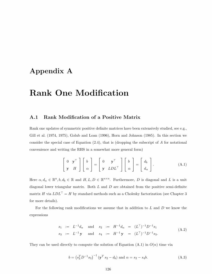
Appendix A
Rank One Modification
A.1 Rank Modification of a Positive Matrix
Rank one updates of symmetric positive definite matrices have been extensively studied, see e.g.,
Gill et al. (1974, 1975), Golub and Loan (1996), Horn and Johnson (1985). In this section we
consider the special case of Equation (2.4), that is (dropping the subscript of A for notational
convenience and writing the RHS in a somewhat more general form)
0 y>
y H
b
α
=
0 y>
y LDL>
b
α
=
db
dα
. (A.1)
Here α, dα ∈ Rn, b, db ∈ R and H,L,D ∈ Rn×n. Furthermore, D is diagonal and L is a unit
diagonal lower triangular matrix. Both L and D are obtained from the positive semi-definite
matrix H via LDL> = H by standard methods such as a Cholesky factorization (see Chapter 3
for more details).
For the following rank modifications we assume that in addition to L and D we know the
expressions
s1 := L−1dα and s2 := H−1dα = (L>)−1D−1s1
s3 := L−1 y and s4 := H−1 y = (L>)−1D−1s3.(A.2)
They can be used directly to compute the solution of Equation (A.1) in O(n) time via
b =(sT3D
−1s3)−1
(yT s2 − db) and α = s2 − s4b. (A.3)
126
A.1 Rank Modification of a Positive Matrix 127
A.1.1 Rank One Extension
After a rank one extension of H, y and dα in Equation (2.4) the augmented system of equations
is given by 0 y>
y H
b
α
=
0 y>
y LDL>
b
α
=
db
dα
, (A.4)
where dα :=
dα
dα
, y :=
y
y
, and H :=
H h
h> h
. Here h, y, dα ∈ R are scalars and
h ∈ Rn is a column vector. L and D can be computed using well known rank one updates
(Golub and Loan, 1996), and we obtain
LDL> =
L
l> 1
D
d
L> l
1
(A.5)
where l = D−1L−1 h and d = h− l>D l. Since L is lower triangular and D is diagonal, L and D
can be computed in O(n2) time. Finally, we can compute the augmented versions of s1, . . . , s4
as follows
s1 =
s11
s12
=
s1old
dα − l> s1old
and s2 =
s2old − (L>)−1 l s12/d
s12/d
s3 =
s31
s32
=
s3old
y − l> s3old
and s4 =
s4old − (L>)−1 l s32/d
s32/d
(A.6)
The expensive part of the above updates is the computation of (L>)−1 l, which takes O(n2)
operations. However, given (L>)−1 l updating s1, . . . , s4 takes O(n) time. Hence the entire
update can be carried out in O(n2) time. Also note that analogous relations hold for rank-v
modifications (with v > 1), the only difference being that in this case vectors become matrices
and scalars become vectors or matrices in an obvious fashion.
A.1.2 Rank One Reduction
Assume that we want to delete the jth row and column from H and reduce Equation (A.1)
correspondingly. This operation occurs when we need to remove a point from the set of Support
Vectors. The following matrix manipulations are standard in numerical analysis and we refer
A.1 Rank Modification of a Positive Matrix 128
the reader to Golub and Loan (1996), Gill et al. (1974, 1975), Horn and Johnson (1985) for
further details. We begin with the decomposition of H into
H =
H11 H12 H13
H21 H22 H23
H31 H32 H33
= LDL>with L =
L11
L21 1
L31 L32 L33
and D =
D1
D2
D3
Straightforward algebra shows that in this case the LDL> decomposition for the reduced matrix H11 H13
H31 H33
satisfies L =
L11
L31 L33
and D =
D1
D3
, where
L33D3L>33 = L33D3L
>33 + L32D2L
>32. (A.7)
Equation (A.7) can be solved in O(n2) operations (where H33 ∈ Rn×n): we first reduce Equa-
tion (A.7) to the problem of factorizing the rank-1 update of a diagonal matrix via
(L−1
33 L33
)D3
(L−1
33 L33
)>= D3 +
(L−1
33 L32
)D2
(L−1
33 L32
)>. (A.8)
Here(L−1
33 L32
)can be computed in O(n2) time (L32 is a vector and L33 is lower triangular).
It turns out that a factorization of the RHS of Equation (A.8) can be obtained in O(n) space
and time (see Golub and Loan (1996), Horn and Johnson (1985)) and we obtain
LD3L> = D3 +
(L−1
33 L32
)D2
(L−1
33 L32
)> where Lij =
0 if i < j
1 if i = j
ζiβj if i > j
(A.9)
What remains is to compute L33 = L33L. In the following we show that this again can be done
in O(n2) time, despite the fact that we have to multiply two lower triangular matrices. We have
[L33
]ij
=[L33L
]ij
= [L33]ij +i∑
l=j+1
[L33]il ζlβj [L33]ij +
i∑l=j+1
[L33]il ζl
βj . (A.10)
Note that all possible terms in the above sum can be computed at O(n2) time simply by starting
with j = i− 1 and progressing to j = 1. Here each step requires O(1) operations.
Now we turn to the updates required for s1, . . . , s4. We can write a stored quantity si as

A.2 Rank-Degenerate Kernels 129
si = [si1, sij , si3]>, where sij is the jth element of the si vector. The updated values are given
by
s1 =
s11
s∗13
=
s11
L−133 (1−L31s11)
s2 =
s∗21
s∗23
=
D−11 (L>11)
−1(s11 −D1L>31s
∗23)
D−13 (L>33)
−1s∗13
s3 =
s31
s∗33
=
s31
L−133 (y3−L31s31)
s4 =
s∗41
s∗43
=
D−11 (L>11)
−1(s31 −D1L>31s
∗43)
D−13 (L>33)
−1s∗33
(A.11)
Since L11 and L33 are triangular matrices the stored quantities can be updated in O(n2) time.
A.2 Rank-Degenerate Kernels
In the case of rank-degenerate kernel we can apply the ideas discussed in Chapter 3 in order to
compute a LDL> decomposition of K in O(nm2) time. Rank-one updates of such a decompo-
sition can be performed in O(mn) time. Details can be found in Section 3.4 as well as in Smola
and Vishwanathan (2003). The procedure to update the stored quantities remains unchanged
in this case.

Bibliography
A. V. Aho, R. Sethi, and J. D. Ullman. Compilers: Principles, Techniques, And Tools.
Addison-Wesley Longman Publishing Co., Inc., Reading, MA, USA, 1986.
A. Amir, M. Farach, Z. Galil, R. Giancarlo, and K. Park. Dynamic dictionary matching.
Journal of Computer and System Science, 49(2):208–222, October 1994.
I. D. Baxter, A. Yahin, L. Moura, M. Sant’Anna, and L. Bier. Clone detection using ab-
stract syntax trees. In Proceedings of International Conference on Software Maintenance,
pages 368–377, Bethesda, Maryland, USA, November 1998. IEEE Press.
J. M. Bennett. Triangular factors of modified matrices. Numerical Mathematics, 7:217–
221, 1965.
K. P. Bennett and O. L. Mangasarian. Multicategory separation via linear programming.
Optimization Methods and Software, 3:27–39, 1993.
J. L. Bentley and M. I. Shamos. Divide-and-conquer in multidimensional space. In Pro-
ceedings of the 8th annual ACM symposium on Theory of computing, pages 220–230, 1976.
C. L. Blake and C. J. Merz. UCI repository of machine learning databases, 1998. URL
http://www.ics.uci.edu/~mlearn/MLRepository.html.
B. E. Boser, I. M. Guyon, and V. N. Vapnik. A training algorithm for optimal margin
classifiers. In D. Haussler, editor, Proceedings of the Annual Conference on Computational
Learning Theory, pages 144–152, Pittsburgh, PA, July 1992. ACM Press.
D. Breslauer. The suffix tree of a tree and minimizing sequential transducers. Theoritical
Computer Science, 191((1-2)):131–144, January 1998.
130

BIBLIOGRAPHY 131
C. J. C. Burges. A tutorial on support vector machines for pattern recognition. Data
Mining and Knowledge Discovery, 2(2):121–167, 1998.
C. J. C. Burges and V. Vapnik. A new method for constructing artificial neural networks.
Interim technical report, ONR contract N00014-94-c-0186, AT&T Bell Laboratories, 1995.
A. Cannon, J. M. Ettinger, D. Hush, and C. Scovel. Machine learning with data dependent
hypothesis classes. Journal of Machine Learning Research, 2:335–358, February 2002.
G. Cauwenberghs and T. Poggio. Incremental and decremental support vector machine
learning. In T. K. Leen, T. G. Dietterich, and V. Tresp, editors, Advances in Neural
Information Processing Systems 13, pages 409–415. MIT Press, 2001.
W. I. Chang and E. L. Lawler. Sublinear approximate sting matching and biological
applications. Algorithmica, 12(4/5):327–344, 1994.
R. Cole and R. Hariharan. Faster suffix tree construction with missing suffix links. In Pro-
ceedings of the Thirty Second Annual Symposium on the Theory of Computing, Portland,
OR, USA, May 2000. ACM.
M. Collins and N. Duffy. Convolution kernels for natural language. In T. G. Dietterich,
S. Becker, and Z. Ghahramani, editors, Advances in Neural Information Processing Sys-
tems 14, Cambridge, MA, 2001. MIT Press.
C. Cortes. Prediction of Generalization Ability in Learning Machines. PhD thesis, De-
partment of Computer Science, University of Rochester, 1995.
C. Cortes and V. Vapnik. Support vector networks. Machine Learning, 20:273–297, 1995.
R. Courant and D. Hilbert. Methods of Mathematical Physics, volume 1. Interscience
Publishers, Inc, New York, 1953.
R. Courant and D. Hilbert. Methods of Mathematical Physics, volume 2. Interscience
Publishers, Inc, New York, 1962.
T. M. Cover and P. E. Hart. Nearest neighbor pattern classifications. IEEE Transactions
on Information Theory, 13(1):21–27, 1967.

BIBLIOGRAPHY 132
N. Cristianini and J. Shawe-Taylor. An Introduction to Support Vector Machines. Cam-
bridge University Press, Cambridge, UK, 2000.
A. P. Dempster, N. M. Laird, and D. B. Rubin. Maximum Likelihood from Incomplete
Data via the EM Algorithm. Journal of the Royal Statistical Society B, 39(1):1–22, 1977.
Richard O. Duda, Peter E. Hart, and David G. Stork. Pattern Classification and Scene
Analysis. John Wiley and Sons, New York, 2001. Second edition.
R. Durbin, S. Eddy, A. Krogh, and G. Mitchison. Biological Sequence Analysis: Proba-
bilistic models of proteins and nucleic acids. Cambridge University Press, 1998.
B. Efron. The jacknife, the bootstrap, and other resampling plans. SIAM, Philadelphia,
1982.
B. Efron and R. J. Tibshirani. An Introduction to the Bootstrap. Chapman and Hall, New
York, 1994.
Bradley Efron and Robert Tibshirani. Improvements on cross-validation: the .632+ boot-
strap method. Journal of the American Statistical Association, 92:548–560, 1997.
E. Eskin, A. Arnold, M Prerau, L Portnoy, and S Stolfo. A geometric framweork for
unsupervised anomaly detection: Detecting intrusions in unlabeled data. In Proceedings
of the Workshop on Data Mining for Security Applications, Philadelphia, PA, November
2001. ACM, Kluwer.
B. S. Everitt. An Introduction to Latent Variable Models. Chapman and Hall, London,
1984.
William Feller. An Introduction To Probability Theory and Its Application, volume 1. John
Wiley and Sons, New York, 1950.
M. C. Ferris and T. S. Munson. Interior point methods for massive support vector ma-
chines. Data Mining Institute Technical Report 00-05, Computer Sciences Department,
University of Wisconsin, Madison, Wisconsin, 2000.
S. Fine and K. Scheinberg. Efficient SVM training using low-rank kernel representations.
Journal of Machine Learning Research, 2:243–264, Dec 2001. http://www.jmlr.org.
BIBLIOGRAPHY 133
R. Fletcher. Practical Methods of Optimization. John Wiley and Sons, New York, 1989.
R. Fletcher and M. J. D. Powell. On the modification of LDL> factorizations. Mathematics
of Computation, 28(128):1067–1087, 1974.
E. Fredkin. Trie memory. Communications of the ACM, 3(9):490–499, September 1960.
Y. Freund and R. E. Schapire. Large margin classification using the perceptron algorithm.
Machine Learning, 37(3):277–296, 1999.
J. D. Gardiner, A. L. Laub, J. J. Amato, and C. B. Moler. Solution of the Sylvester
matrix equation AXB> +CXD> = E. ACM Transactions on Mathematical Software, 18
(2):223–231, 1992.
T. Gartner, P. A. Flach, A. Kowalczyk, and A. J. Smola. Multi-instance kernels. In
Proceedings of the 19th International Conference on Machine Learning ICML, 2002.
R. Giancarlo. A generalization of the suffix tree to matrices,with applications. SIAM
Journal on Computing, 24(3):520–562, 1995.
R. Giancarlo and R. Grossi. On the construction of classes of suffix trees for square
matrices: Algorithms and applications. Information and Computation, 130:151–182, 1996.
R. Giancarlo and R. Grossi. Parallel construction and query of index data structures for
pattern matching and square matrices. Journal of Complexity, 15:30–71, 1997.
R. Giancarlo and R. Guaiana. On-line construction of two dimensional suffix trees. Journal
of Complexity, 15:72–127, 1999.
R. Giegerich and S. Kurtz. From Ukkonen to McCreight and Weiner: A unifying view of
linear-time suffix tree construction. Algorithmica, 19(3):331–353, 1997.
P. E. Gill, G. H. Golub, W. Murray, and M. A. Saunders. Methods for modifying matrix
factorizations. Mathematics of Computation, 28(126):505–535, April 1974.
P. E. Gill, W. Murray, and M. A. Saunders. Methods for computing and modifying the
LDV factors of a matrix. Mathematics of Computation, 29(132):1051–1077, October 1975.
BIBLIOGRAPHY 134
P. E. Gill, W. Murray, M. A. Saunders, and M. H. Wright. Inertia-controlling methods
for general quadratic programming. SIAM Review, 33(1), March 1991.
A. Gionis, P. Indyk, and R. Motwani. Similarity search in high dimensions via hashing.
In M. P. Atkinson, M. E. Orlowska, P. Valduriez, S. B. Zdonik, and M. L. Brodie, editors,
Proceedings of the 25th VLDB Conference, pages 518–529, Edinburgh, Scotland, 1999.
Morgan Kaufmann.
D. Goldfarb and K. Scheinberg. A product-form Cholesky factorization method for han-
dling dense columns in interior point methods for linear programming. Technical report,
IBM Watson Research Center, Yorktown Heights, 2001.
G. H. Golub and C. F. Van Loan. Matrix Computations. John Hopkins University Press,
Baltimore, MD, 3rd edition, 1996.
F. C. Graham. Logarithmic Sobolev techniques for random walks on graphs. In D. A.
Hejhal, J. Friedman, M. C. Gutzwiller, and A. M. Odlyzko, editors, Emerging Applications
of Number Theory, number 109 in IMA Volumes in Mathematics and its Applications,
pages 175–186. Springer, 1999. ISBN 0-387-98824-6.
M. Gribskov and N. L. Robinson. Use of receiver operating characteristic (ROC) analysis
to evaluate sequence matching. Computers and Chemistry, 20(1):25–33, 1996.
R. Grossi and G. Italiano. Suffix trees and their applications in string algorithms. In
Procedings of 1st South American Workshop on String Processing (WSP 1993), pages
57–76, September 1993.
D. Gusfield. Algorithms on Strings, Trees and Sequences: Computer Science and Compu-
tational Biology. Cambridge University Press, June 1997. ISBN 0-521-58519-8.
Y. Hamamoto, S. Uchimura, and S. Tomita. A bootstrap technique for nearest neighor
classifier design. IEEE Transactions on Pattern Analysis and Machine Intelligence, 19(1):
73–79, January 1997.
D. Haussler. Convolutional kernels on discrete structures. Technical Report UCSC-CRL-
99-10, Computer Science Department, UC Santa Cruz, 1999.
BIBLIOGRAPHY 135
S. Haykin. Neural Networks : A Comprehensive Foundation. Macmillan, New York, 1994.
R. Herbrich. Learning Kernel Classifiers: Theory and Algorithms. MIT Press, 2002.
M. Herbster. Learning additive models online with fast evaluating kernels. In D. P.
Helmbold and B. Williamson, editors, Proceedings of the Fourteenth Annual Conference
on Computational Learning Theory (COLT), volume 2111 of Lecture Notes in Computer
Science, pages 444–460. Springer, 2001.
M. W. Hirsch and S. Smale. Differential equations, dynamical systems, and linear algebra.
Academic Press, New York, 1974.
J. E. Hopcroft and J. D. Ullman. Introduction to Automata Theory, Languages and Com-
putation. Addison-Wesley, Reading, Massachusetts, first edition, 1979.
T. Hopkins. Remark on algorithm 705: A fortran-77 software package for solving the
Sylvester matrix equation AXB> + CXD> = E. ACM Transactions on Mathematical
Software (TOMS), 28(3):372–375, 2002.
R. A. Horn and C. R. Johnson. Matrix Analysis. Cambridge University Press, Cambridge,
1985.
P. Indyk and R. Motawani. Approximate nearest neighbors: Towards removing the curse
of dimensionality. In Proceedings of the 30th Symposium on Theory of Computing, pages
604–613, 1998.
T. S. Jaakkola, M. Diekhans, and D. Haussler. Using the Fisher kernel method to detect
remote protein homologies. In Proceedings of the International Conference on Intelligence
Systems for Molecular Biology, pages 149–158. AAAI Press, 1999.
T. S. Jaakkola, M. Diekhans, and D. Haussler. A discriminative framework for detecting
remote protein homologies. Journal of Computational Biology, 7:95–114, 2000.
T. Joachims. Text categorization with support vector machines: Learning with many
relevant features. In Proceedings of the European Conference on Machine Learning, pages
137–142, Berlin, 1998. Springer.

BIBLIOGRAPHY 136
T. Joachims. Making large-scale SVM learning practical. In B. Scholkopf, C. J. C. Burges,
and A. J. Smola, editors, Advances in Kernel Methods—Support Vector Learning, pages
169–184, Cambridge, MA, 1999. MIT Press.
T. Joachims. Learning to Classify Text Using Support Vector Machines: Methods, Theory,
and Algorithms. The Kluwer International Series In Engineering And Computer Science.
Kluwer Academic Publishers, Boston, May 2002. ISBN 0-7923-7679-X.
T. Joachims, N. Cristianini, and J. Shawe-Taylor. Composite kernels for hypertext cate-
gorisation. In C. Brodley and A. Danyluk, editors, Proceedings of the 18th International
Conference on Machine Learning (ICML), pages 250–257, San Francisco, US, 2001. Mor-
gan Kaufmann.
L. Kaufman. Solving the quadratic programming problem arising in support vector clas-
sification. In B. Scholkopf, C. J. C. Burges, and A. J. Smola, editors, Advances in Kernel
Methods—Support Vector Learning, pages 147–168, Cambridge, MA, 1999. MIT Press.
S. S. Keerthi, S. K. Shevade, C. Bhattacharyya, and K. R. K. Murthy. A fast iterative
nearest point algorithm for support vector machine classifier design. Technical Report
Technical Report TR-ISL-99-03, Indian Institute of Science, Bangalore, 1999. URL http:
//guppy.mpe.nus.edu.sg/~mpessk/npa_tr.ps.gz.
S. S. Keerthi, S. K. Shevade, C. Bhattacharyya, and K. R. K. Murthy. A fast iterative
nearest point algorithm for support vector machine classifier design. IEEE Transactions
on Neural Networks, 11(1):124–136, January 2000.
D. K. Kim and K. Park. Linear-time construction of two-dimensional suffix trees. In Pro-
ceedings of the 26th International Colloquium on Automata, Languages and Programming
(ICALP), volume 1644 of LNCS, pages 463–472, Prague, Czech, July 1999. Springer.
D. E. Knuth. The Art of Computer Programming: Fundamental Algorithms, volume 1.
Addison-Wesley, Reading, Massachusetts, second edition, 1998a.
D. E. Knuth. The Art of Computer Programming: Sorting and Searching, volume 3.
Addison-Wesley, Reading, Massachusetts, second edition, 1998b.
BIBLIOGRAPHY 137
Ron Kohavi. A study of cross validation and bootstrap for accuracy estimation and model
selection. In Proceedings of the International Joint Conference on Neural Networks, 1995.
R. S. Kondor and J. Lafferty. Diffusion kernels on graphs and other discrete structures.
In Proceedings of the ICML, 2002.
Y. LeCun, L. D. Jackel, L. Bottou, C. Cortes, J. S. Denker, H. Drucker, I. Guyon, U. A.
Muller, E. Sackinger, P. Simard, and V. Vapnik. Learning algorithms for classification: A
comparison on handwritten digit recognition. Neural Networks, pages 261–276, 1995.
E. Leopold and J. Kindermann. Text categorization with support vector machines: How
to represent text in input space? Machine Learning, 46(3):423–444, March 2002.
C. Leslie, E. Eskin, and W. S. Noble. The spectrum kernel: A string kernel for SVM
protein classification. In Proceedings of the Pacific Symposium on Biocomputing, pages
564–575, 2002a.
C. Leslie, E. Eskin, J. Weston, and W. S. Noble. Mismatch string kernels for SVM protein
classification. In Proceedings of Neural Information Processing Systems 2002, 2002b. in
press.
H. Lodhi, C. Saunders, J. Shawe-Taylor, N. Cristianini, and C. Watkins. Text classification
using string kernels. Journal of Machine Learning Research, 2:419–444, February 2002.
D. G. Luenberger. Introduction to Dynamic Systems: Theory, Models, and Applications.
John Wiley and Sons, Inc., New York, USA, May 1979. ISBN 0-471-02594-1.
L. M. Manevitz and M. Yousef. One-class SVMs for document classification. Journal of
Machine Learning Research, 2:139–154, December 2001.
O. L. Mangasarian. Nonlinear Programming. McGraw-Hill, New York, 1969.
O. L. Mangasarian and D. R. Musicant. Lagrangian support vector machines. Journal of
Machine Learning Research, 1:161–177, 2001. http://www.jmlr.org.
E. M. McCreight. A space-economical suffix tree construction algorithm. Journal of the
ACM, 23(2):262–272, April 1976.

BIBLIOGRAPHY 138
P. Niyogi, F. Girosi, and T. Poggio. Incorporating prior knowledge in machine learning
by creating virtual examples. Proceedings of IEEE, 86(11):2196–2209, November 1998.
K. Oflazer. Error-tolerant retrieval of trees. IEEE Transactions on Pattern Analysis and
Machine Intelligence, 19(12):1376–1380, December 1997.
M. Opper and O. Winther. Gaussian processes and SVM: Mean field and leave-one-out.
In A. J. Smola, P. L. Bartlett, B. Scholkopf, and D. Schuurmans, editors, Advances in
Large Margin Classifiers, pages 311–326, Cambridge, MA, 2000. MIT Press.
E. Osuna, R. Freund, and F. Girosi. An improved training algorithm for support vector
machines. In J. Principe, L. Gile, N. Morgan, and E. Wilson, editors, Neural Networks
for Signal Processing VII—Proceedings of the 1997 IEEE Workshop, pages 276–285, New
York, 1997. IEEE.
A. Parker and J. O. Hamblen. Computer algorithms for plagiarism detection. IEEE
Transactions on Education, 32(2):94–99, May 1989.
J. Platt. Fast training of support vector machines using sequential minimal optimization.
In B. Scholkopf, C. J. C. Burges, and A. J. Smola, editors, Advances in Kernel Methods—
Support Vector Learning, pages 185–208, Cambridge, MA, 1999. MIT Press.
M. Revow, C. K.I. Williams, and G. E. Hinton. Using generative models for handwritten
digit recognition. IEEE Transactions on Pattern Analysis and Machine Intelligence, 18
(6):592–606, 1996.
D. Roobaert. DirectSVM: A simple support vector machine perceptron. In Neural Net-
works for Signal Processing X—Proceedings of the 2000 IEEE Workshop, pages 356–365,
New York, December 2000. IEEE.
B. Scholkopf. Support Vector Learning. R. Oldenbourg Verlag, Munchen, 1997. Doktorar-
beit, TU Berlin. Download: http://www.kernel-machines.org.
B. Scholkopf, A. Smola, R. C. Williamson, and P. L. Bartlett. New support vector algo-
rithms. Neural Computation, 12:1207–1245, 2000.
B. Scholkopf and A. J. Smola. Learning with Kernels. MIT Press, 2002.

BIBLIOGRAPHY 139
T. Seol and S. Park. Solving linear systems in interior-point methods. Computers and
Operations Research, 29:317–326, 2002.
John Shawe-Taylor, Peter L. Bartlett, Robert C. Williamson, and Martin Anthony. Struc-
tural risk minimization over data-dependent hierarchies. IEEE Transactions on Informa-
tion Theory, 44(5):1926–1940, 1998.
Kristy Sim. Context kernels for text categorization. Master’s thesis, The Australian
National University, Canberra, Australia, ACT 0200, June 2001.
A. J. Smola and B. Scholkopf. A tutorial on support vector regression. NeuroCOLT
Technical Report NC-TR-98-030, Royal Holloway College, University of London, UK,
1998.
A. J. Smola and B. Scholkopf. Sparse greedy matrix approximation for machine learning.
In P. Langley, editor, Proceedings of the International Conference on Machine Learning,
pages 911–918, San Francisco, 2000. Morgan Kaufmann Publishers.
A. J. Smola and S. V. N. Vishwanathan. Cholesky factorization for rank-k modifications
of diagonal matrices. SIAM Journal of Matrix Analysis, 2003. in preparation.
G. W. Stewart. Decompositional approach to matrix computation. Computing in Science
and Engineering, 2(1):50–59, February 2000.
J. Stoer and R. Bulirsch. Introduction to Numerical Analysis. Springer, New York, second
edition, 1993.
G. Strang. Introduction to Linear Algebra. Wellesley-Cambridge Press, August 1998.
E. Ukkonen. On-line construction of suffix trees. Algorithmica, 14(3):249–260, 1995.
P. M. Vaidya. An O(n log(n)) algorithm for the all-nearest-neighbors problem. Discrete
and Computational Geometry, 4(2):101–115, January 1989.
R. J. Vanderbei. LOQO: An interior point code for quadratic programming. TR SOR-94-
15, Statistics and Operations Research, Princeton Univ., NJ, 1994.
R. J. Vanderbei. Linear Programming: Foundations and Extensions. Kluwer Academic,
Hingham, 1997.

BIBLIOGRAPHY 140
V. Vapnik. The Nature of Statistical Learning Theory. Springer, New York, 1995.
V. Vapnik and A. Chervonenkis. Theory of Pattern Recognition [in Russian]. Nauka,
Moscow, 1974. (German Translation: W. Wapnik & A. Tscherwonenkis, Theorie der
Zeichenerkennung, Akademie-Verlag, Berlin, 1979).
S. V. N. Vishwanathan and M. N. Murty. Geometric SVM: A fast and intuitive SVM
algorithm. In Proceedings of the ICPR, 2002a. accepted.
S. V. N. Vishwanathan and M. N. Murty. Jigsawing: A method to generate virtual
examples in OCR data. In Proceedings of the Second International Conference on Hybrid
Intelligent Systems, 2002b. To appear.
S. V. N. Vishwanathan and M. N. Murty. Jigsawing: A method to generate virtual
examples in OCR data. Pattern Recognition, 2002c. under preparation.
S. V. N. Vishwanathan and M. N. Murty. Use of MPSVM for data set reduction. In
A. Abraham and M. Koeppen, editors, Hybrid Information Systems, Heidelberg, 2002d.
Physica Verlag.
S. V. N. Vishwanathan and M. N. Murty. Use of MPSVM for data set reduction. In
A. Abraham, L. Jain, and J. Kacprzyk, editors, Recent Advances in Intelligent Paradigms
and Applications, volume 113 of Studies in Fuzziness and Soft Computing, chapter 16.
Springer Verlag, Berlin, November 2002e.
S. V. N. Vishwanathan and A. J. Smola. Kernels on structured objects. Technical report,
Australian National University, RSISE, 2002. in preparation.
P. Viswanath and M. N. Murty. An efficient incremental mining algorithm for compact
realization of prototypes. Technical Report IISC-CSA-2002-2, CSA Department, Indian
Institute of Science, Bangalore, India, January 2002.
C. Watkins. Dynamic alignment kernels. In A. J. Smola, P. L. Bartlett, B. Scholkopf, and
D. Schuurmans, editors, Advances in Large Margin Classifiers, pages 39–50, Cambridge,
MA, 2000. MIT Press.
BIBLIOGRAPHY 141
P. Weiner. Linear pattern matching algorithms. In Proceedings of the IEEE 14th Annual
Symposium on Switching and Automata Theory, pages 1–11, The University of Iowa, 1973.
IEEE.
E. Weyer. System Identification in the Behavioural Framework. PhD thesis, The Norwegian
Institute of Technology, Trondheim, 1992.
J. C. Willems. From time series to linear system. I. Finite-dimensional linear time invariant
systems. Automatica J. IFAC, 22(5):561–580, 1986a.
J. C. Willems. From time series to linear system. II. Exact modelling. Automatica J.
IFAC, 22(6):675–694, 1986b.
J. C. Willems. From time series to linear system. III. Approximate modelling. Automatica
J. IFAC, 23(1):87–115, 1987.
C. K. I. Williams and M. Seeger. The effect of the input density distribution on kernel-
based classifiers. In P. Langley, editor, Proceedings of the International Conference on
Machine Learning, pages 1159–1166, San Francisco, California, 2000. Morgan Kaufmann
Publishers.
T. Zhang. Some sparse approximation bounds for regression problems. In Proc. 18th Inter-
national Conf. on Machine Learning, pages 624–631. Morgan Kaufmann, San Francisco,
CA, 2001.