eﬃcient kernel density estimation using the fast gauss...

Efficient Kernel Density Estimation Using the

Fast Gauss Transform with Applications to

Segmentation and Tracking

Ahmed Elgammal, Ramani Duraiswami, Larry S. DavisComputer Vision LaboratoryThe University of Maryland

College Park, MD 20742, USA

Abstract

The study of many vision problems is reduced to the estimation of a proba-bility density function from observations. Kernel density estimation techniquesare quite general and powerful methods for this problem, but have a significantdisadvantage in that they are computationally intensive. In this paper we ex-plore the use of kernel density estimation with the fast gauss transform (FGT)for problems in vision. The FGT allows the summation of a mixture of M Gaus-sians at N evaluation points in O(M + N) time as opposed to O(MN) timefor a naive evaluation, and can be used to considerably speed up kernel densityestimation. We present applications of the technique to problems from imagesegmentation and tracking, and show that the algorithm allows application ofadvanced statistical techniques to solve practical vision problems in real timewith today’s computers.

1 Introduction

Many problems in computer vision can be posed as obtaining the probabilitydensity function describing an observed random quantity. In general the formsof the underlying density functions are not known. While classical parametricdensities are mostly unimodal, practical computer vision problems involve mul-timodal densities. Further, high-dimensional densities can not often be simplyrepresented as the product of one-dimensional density functions. While mix-ture methods partially alleviate this problem, they require knowledge aboutthe problem to choose the number of mixture functions, and their individualparameters.

An attractive feature of nonparametric procedures is that they can be usedwith arbitrary distributions and without the assumption that the forms of the

1

2nd Int’l workshop on Statistical and Computational Theories of Vision 2

underlying densities are known. However, most nonparametric methods requirethat all of the samples be stored or that the designer have extensive knowledgeof the problem. Since a large number of samples is needed to obtain goodestimates, the memory requirements can be severe [1].

A particular nonparametric technique that estimates the underlying densityand is quite general is the kernel density estimation technique. In this techniquethe underlying probability density function is estimated as

f(x) =∑

i

αiK(x− xi) (1)

where K is a “kernel function” (typically a Gaussian) centered at the datapoints, xi, i = 1..n and αi are weighting coefficients (typically uniform weightsare used, i.e., αi = 1/n). Note that choosing the Gaussian as a kernel function isdifferent from fitting the distribution to a Gaussian model. Here, the Gaussianis only used as a function that is weighted around the data points. The use ofsuch an approach requires a way to efficiently evaluate the estimate f(xj) atany new point xj . A good discussion of kernel estimation techniques can befound in [2].

In general, given N original data samples and M points at which the den-sity must be evaluated, the complexity is O(NM) evaluations of the kernelfunction, multiplications and additions. For many applications in computer vi-sion, where both real-time operation and generality of the classifier are desired,this complexity can be a significant barrier to the use of these density estimationtechniques. In this paper we discuss the application of an algorithm, the FastGauss Transform (FGT) [3, 4], that improves the complexity of this evaluationto O(N +M) operations, to computer vision problems.

The FGT is one of a class of very interesting and important new familiesof fast evaluation algorithms that have been developed over the past dozenyears, and are revolutionizing numerical analysis. These algorithms use the factthat all computations are required only to a certain accuracy (which can bearbitrary) to speed up calculations. These algorithms enable rapid calculationof approximations of arbitrary accuracy to matrix-vector products of the formAd where aij = φ(|xi − xj |) and φ is a particular special function. Thesesums first arose in applications that involve potential fields where the functionsφ were spherical harmonics, and go by the collective name “fast multipole”methods [3]. The basic idea is to cluster the sources and target points usingappropriate data structures, and to replace the sums with smaller summationsthat are equivalent to a given level of precision. Interesting applications of thesealgorithms include fast versions of Fourier transforms that do not require evenlyspaced data points [5]. An algorithm for evaluating Gaussian sums using thistechnique was developed by Greengard and Strain [4]. We will be concernedwith this algorithm and its extensions in this paper. Related work also includesthe work by Lambert et al [6] for efficient on-line computation of kernel densityestimation.

Section 2 introduces some details of the Fast Gauss Transform, and our im-provements to it. We also present practical demonstrations of the improvement


in complexity. In Section 3 we introduce using kernel density estimation tomodel the color of homogenous regions and use this approach to segment fore-ground region corresponding to people into major body parts. In Section 4 weshow how the fast Gauss algorithm can be used to efficiently compute estimatesfor density gradient and use this for tracking people. The tracking algorithm isrobust to partial occlusion and rotation in depth and can be used with station-ary or moving cameras. Appropriate reviews of the relevant related work areprovided in these self-contained sections.

2 Fast Gauss Transform

The FGT was introduced by Greengard and Strain [3, 4] for the rapid evaluationof sums of the form

S (ti) =N∑

j=1

fj exp

(− (sj − ti)

2

σ2

), i = 1, . . . ,M. (2)

Here sj and ti are respectively the d−dimensional “source” and “target” coor-dinates, while σ is a scalar and fj are source strengths. They showed that usingtheir fast algorithm this sum could be computed in O(N+M) operations. Theyalso showed results from 1-D and 2-D tests of the algorithm. It was extended byStrain [7] to sums where σ in equation 2 varied with the position of the targetor the source, i.e., for the case where σ depends on the source location the sumis

S (ti) =N∑

j=1

fj exp

(− (sj − ti)

2

σ2j

), i = 1, . . . ,M. (3)

A puzzling aspect of the FGT is that even though the algorithm was pub-lished fourteen years ago, and Gaussian mixture sums arise often in statistics(as already noted by Greengard and Strain), the algorithm has not been usedmuch in applications. Subsequent publications on the FGT have only begun toappear again over the last two years.

An important reason for the lack of use of the algorithm is probably thefact that it is inconvenient to do so. First, it is not immediately clear what thecross-over point is when the algorithm begins to manifest its superior asymptoticcomplexity and offsets the pre-processing overhead. While the nominal complex-ity of the algorithm is O(M + N),the constant multiplying it is O(pd), wherep is the number of retained terms in a polynomial approximation (describedbelow). This makes it unclear if the algorithm is useful for higher dimensionapplications seen in statistical pattern recognition. The fact that there is noreadily available implementation to test these issues acts as a further barrier toits wide adoption.

Another reason for the delay in applying the FGT to problems in compu-tational statistics might be that the algorithm, as originally presented, are notdirectly applicable to general mixture of gaussian sums that statisticians are


used to thinking about. General d−dimensional mixture of gaussian sums havethe form

S(ti) =N∑

j=1

fj exp(− (ti − sj)

′V −1 (ti − sj)

)(4)

with V −1 is a symmetric positive definite covariance matrix, which is much morecomplex than 2. Even in the case of kernel density estimation with Gaussians,the form of the Gaussian sum encountered is

S(ti) =N∑

j=1

fje−∑d

k=1

((ti−sj)k

σk

)2

=N∑

j=1

fje−[(

(ti−sj)1σ1

)2

+...+

((ti−sj)d

σd

)2], (5)

where the subscript k indicates the component along the kth coordinate axis,i.e., the covariance matrix is diagonal. The applications we present below insegmentation and tracking use this form which is a generalization over the orig-inal FGT algorithm. Our ongoing work (the details of which, including a proofof convergence are to be reported elsewhere) extends the variable scale FGTalgorithm to sums of the form 5.

2.1 Speeding up computations with Gaussians

Before describing the FGT, it is appropriate to describe some algorithmic im-provements for evaluating Gaussian mixture sums proposed in the literature,which are distinct from the FGT.

The evaluation of a special function such as the exponential is usually ex-pensive, requiring ˜O(100) floating point operations using the normal librariessupplied with compilers. Approximate libraries that achieve accuracy almosteverywhere, and require fewer floating point operations are available, e.g., theIntel approximate math library [8] claims a speedup of a factor of 5 for eval-uating exponentials over the corresponding x87 implementation. The FGT isdistinct from these, and indeed the approximate math libraries can be used inconjunction with it to achieve further speed-up.

A second speed-up of gaussian sums is based on the observation that sincea Gaussian typically decays relatively quickly, leading to insignificant additionswhen it is evaluated beyond a specified distance, heuristics can be used to avoidunnecessary evaluations when σ−1 (|s− t|) is small. Some authors (e.g., Fritsch& Rogina, 1996 [9]) have formalized this by developing a data structure thatenables automating this heuristic. The FGT also employs such data structures,and automates the observation that lies behind this heuristic by providing rig-orous error bounds.


2.2 Overview of the Algorithm

The shifting identity that is central to the algorithm is a re-expansion of theexponential in terms of a Hermite series by using the identity

e−( t−sσ )2

= e−(

t−s0−(s−s0)σ

)2

= e−( t−s0σ )2

∞∑n=0

1n!

(s− s0σ

)n

Hn

(t− s0σ

), (6)

where Hn are the Hermite polynomials. This formula tells us how to evaluatethe Gaussian field exp

(− ( t−s

σ

)2)at the target t due to the source at s, as anHermite expansion centered at any given point s0. Thus a Gaussian centered ats can be shifted to a sum of Hermite polynomials times a Gaussian, all centeredat s0. The series converges rapidly and for a given precision only p terms needto be retained. The quantities t and s can be interchanged to obtain a Taylorseries around the target location as

e−( t−sσ )2

= e−(

t−t0−(s−t0)σ

)2

�p∑

n=0

1n!hn

(s− t0σ

)(t− t0σ

)n

. (7)

where the Hermite functions hn (t)are defined by

hn (t) = e−t2Hn (t) . (8)

The algorithm achieves its gain in complexity by avoiding evaluating everyGaussian at every evaluation point (which leads to O(NM) operations). Rather,equivalent p term series are constructed about a small number of source cluster-centers using Equation 6 (for O(Npd) operations). These series are then shiftedto target cluster-centers, and evaluated at the M targets in O(Mpd) operations.Here the number of terms in the series evaluations, p, is related to the desiredlevel of precision ε, and is typically small as these series converge quickly.

The process is illustrated in Figure 1. The sources and targets are dividedinto clusters using a simple boxing operation. This permits the division of theGaussians according to their locations The domain is scaled to be of O(1), andthe box sizes are chosen to be of size r

√2σ where r is a scale parameter.

Since Gaussians decay rapidly, sources in a given box will have no effect (interms of the desired accuracy) to targets relatively far from there sources (interms of distance scaled by the standard deviation σ). Therefore the effect ofsources in a given box need to be computed only for targets in close boxes. Giventhe sources in one box and the targets in a neighboring box, the computationis performed using one of the following four methods depending on the numberof sources and targets in these boxes: Direct evaluation is used if the numberof sources and targets are small. If the sources are clustered in a box thenthey can be transformed into Hermite expansion about the center of the boxusing equation 6. This expansion is directly evaluated at each target if thenumber of the targets is small. If the targets are clustered then the sources ortheir expansion are converted to a local Taylor series (equation 7) which is then


Figure 1: The fast gauss transform performs gaussian sums to a prescribeddegree of accuracy by using either direct evaluations of the Gaussian for isolatedsources and targets, or consolidates sources with Hermite series evaluation atisolated targets, or consolidates many sources near a clustered target locationvia Taylor series, or combines Hermite and Taylor series for clustered sourcesand targets.

evaluated at each target in the box. The number of terms to be retained inthe series, p, depends on the required precision, the box size scale parameterr and the standard deviation σ. The break-even point when using expansionis more efficient than direct evaluation is O(pd−1). Further details may beobtained from [4]. The clustering operation is aided by the use of appropriatedata structures.

2.3 Fast Gauss Transform Experimental Results

Before presenting applications of the FGT to vision problems, we present someexperimental results, that illustrate further how the algorithm achieves its speedup.The first experiment compares the performance of the FGT with different choicesof the required precision ε with direct evaluation for a 2D problem. Table 1 andFigure 2 shows the CPU time using direct evaluation versus that using FGTfor different precisions, ε = 10−4, 10−6, and 10−8 for sources with σ = 0.05.


The box size scale parameter r was set to 0.51. The sources and targets wereuniformly distributed in the range [0,1] and the strength of the sources wererandom between 0 and 1. Table 2 shows the division of work between the differ-ent components of the FGT algorithm for the ε = 10−6 case. From the divisionof work we notice that for relatively small number of sources and targets onlydirect evaluation is performed. Although, in this case, the algorithm performsonly direct evaluations, it gives five to ten times speed up when compared withdirect evaluation because of the way the algorithm divides the space into boxesand the locality of the direct evaluation based on the desired precision. i.e.,the FGT algorithm does a smart direct evaluation. This is comparable to thespeed-ups reported by Fritsch and Rogina with their bucket-box data structure.As the number of sources and targets increases and they become more clus-tered, other evaluation decisions are made by the algorithm, and the algorithmstarts to show the linear (O(N + M)) performance. For very large number ofsources and targets, the computation are performed through Hermite expan-sions of sources transformed into Taylor expansions as described above, andthis yields a significant speedup. For example, for N = M = 105, the algorithmgives more than 800 time speedup than direct evaluation for 10−4 precision.

From the figures we also note that the FGT starts to outperform directevaluation for number of sources and targets as low as 60-80 based on the desiredaccuracy. This break-even point can be pushed further down by increasing thebox size scale parameter, r. This will enhance the performance of the algorithmfor small N,M but will worsen the asymptotic performance.

Direct Fast GaussN=M Evaluation ε = 10−4 ε = 10−6 ε = 10−8

50 0.7 0.8 0.9 1.1100 2.7 1.3 1.7 2.0200 10.8 2.9 3.7 4.6400 43 8.2 10.8 14800 174 27 36 461600 689 96 130 1633200 2754 319 493 6406400 11917 660 1281 193512800 58500 942 2022 327725600 234x 103 1429 3210 511351200 936x 103 2405 5602 8781102400 3744x 103 4382 10410 16181204800 14976x 103 8428 20191 311061024000 374x 106 43843 100263 153791

Table 1: Run time in milliseconds for direct evaluation vs. FGT with differentprecision

Figure 3 shows the performance of the algorithm for cases where the sourcesand the targets are clustered differently. The direct evaluation is compared with

1The software was written in Visual C++ and the results were obtained on a 700MHz IntelPentium III PC with 512 MB RAM.


102

103

104

105

106

10−4

10−2

100

102

104

106

N=M

seco

nds

Direct evaluationFGT tol = 1e−8 FGT tol = 1e−6 FGT tol = 1e−4

Figure 2: Run time for direct evaluation vs. FGT with different precision

Division of work (%) - Uniform sources and targets

Direct Taylor Hermit Hermit + TaylorN=M Evaluation Expansion Expansion Expansion

≤ 800 100 0 0 01600 96.6 1.6 1.8 03200 65.7 15.6 15 3.76400 5.3 18.3 16.9 59.512800 0 0.3 0.3 99.4≥ 25600 0 0 0 100

Table 2: Division of work between different computational methods for uni-formly distributed random sources and targets

the FGT for three configurations of sources and targets: in the first case, thesources and targets are uniformly distributed between 0 and 1. In the secondcase the sources are clustered inside a circle of radius 0.1 and the targets areuniformly distributed between 0 and 1. In the third case, both the sourcesand the targets are clustered inside a circle of radius 0.1. For all three cases thedesired precision was set to 10−6, the sources have a scale σ = 0.05 and a randomstrength between 0 and 1. The division of work for the three cases are shownin Tables 2, 3, and 4. From the figures we note that for the cases where sourcesand/or targets are clustered the computation shows linear time behavior fornumber of sources and targets as low as 100, which yields a significant speedup.For a very large number of sources and targets, the computations are performedthrough Hermite expansions of sources transformed into Taylor expansions.

Figure 4 shows the same experiment with the three configurations of sourcesand targets for the 3D case with precision set to 10−6 and r = 0.5. Note that the


102

103

104

105

106

10−4

10−2

100

102

104

106

N=M

seco

nds

Direct evaluation FGT: uniform sources & targets FGT: Clustered sources FGT: Clustered sources & targets

Figure 3: Run time for FGT with different configuration of sources and targetslayout

Division of work (%) - Clustered sources, Uniform targets


100 83.7 0 16.3 0200 65.2 0 34.8 0400 32.7 0 67.3 0800 21.3 0 78.7 01600 17.1 0.3 81.4 1.23200 9.2 2.7 69.2 18.96400 1.8 5.6 22.5 70.112800 0 2.6 0.4 97≥ 25600 0 0 0 100

Table 3: Division of work between different computational methods for clusteredsources and uniformly distributed targets

algorithm starts to utilize computations using Hermite and/or Taylor expansiononly when the number of sources and/or targets in a box exceeds a break pointof order pd−1 which is higher in the 3D case. This causes the algorithm to domostly direct evaluation for the uniform sources and targets case while Hermiteand Taylor expansion computations were utilized for large number of clusteredsources and/or targets.

Figure 5 shows effect of the source scale on the run time of the FGT algo-rithm. The figure shows the run time for three cases where sources have scaleσ = 0.1, 0.05, 0.01. For all the cases, the sources and targets were uniformlydistributed between 0 and 1. The box size scale parameter was set to r = 0.5for all the cases. The run time in all the cases converges asymptotically to thelinear behavior.


Division of work (%) - Clustered sources and targets


100 69.4 13.9 13.9 2.8200 36.9 28.7 19.3 15.1400 12.7 21.6 24.4 41.3800 4.8 16.8 17.4 61.01600 2.8 15.1 13.0 69.13200 2.2 10.3 15.3 72.26400 0.8 6.8 9.3 83.112800 0.1 2.4 2.4 95.1≥ 25600 0 0 2.4 97.6

Table 4: Division of work between different computational methods for clusteredsources and targets

102

103

104

105

10−3

10−2

10−1

100

101

102

103

104

105

N=M

seco

nds

Direct evaluation FGT: uniform sources & targets FGT: clustered sources, uniform FGT:clustered sources & targets

Figure 4: Run time for 3D - FGT with different configuration of sources andtargets layout

3 Region Segmentation via Color Modeling

3.1 Color Density Estimation

In this application we utilize the fast Gauss algorithm for efficient density es-timation of color distribution of a region. We use this approach to model thecolor distribution on people’s clothing and to segment major body parts basedon clothing. A variety of parametric and non-parametric statistical techniqueshave been used to model the color and the spatial properties of colored regions.In [10] the color properties of a region (blob) were modeled using a single Gaus-sian in the three dimensional Y UV space. The use of a single Gaussian tomodel the color of a blob restricts the blob to be of a single color which is not ageneral enough assumption about the clothes people wear which usually contain


102

103

104

105

106

10−4

10−2

100

102

104

106

N=M

seco

nds

Direct EvaluationFGT: scale = 0.1 FGT: scale = 0.05FGT: scale = 0.01

Figure 5: Run time for 2D - FGT with uniformly distributed sources and targetswith different scales.

patterns and have many colors. Fitting a mixture of Gaussian using the EM al-gorithm provides a way to model blobs with a mixture of colors. This techniquewas used in [11, 12] for color based tracking of a single blob and was applied fortracking faces. The mixture of Gaussian technique faces the problem of choosingthe right number of Gaussians for the assumed model. Non-parametric tech-niques using histograms have also been used for modeling color distributgions.In [13] 3-dimensional adaptive histograms in RGB space were used to modelthe color of the whole person. Color histograms have also been used in [14]for tracking hands. The major drawback with color histograms is the lack ofconvergence to the right density function if the data set is small.

We use a non-parametric approach to model the color distribution of a uni-form region. Given a sample S = {xi} taken from the region where i = 1...Nand xi is a d-dimensional vector representing the color, we can estimate thedensity function at any point y of the color space directly from S using kerneldensity estimation [2]

P (y) =1

Nσ1...σd

N∑i=1

d∏j=1

K

(yj − xij

σj

), (9)

where the same kernel function is used in each dimension with a different band-width σj for each dimension of the color space.

Theoretically, kernel density estimators can converge to any density shapewith enough samples [2]. Unlike histograms, even with a small number of sam-ples, kernel density estimation leads to a smooth continuous density estimate. Ifthe underlying distribution is a mixture of Gaussians, kernel density estimationconverges to the right density with a small number of samples. Unlike paramet-ric fitting of a mixture of Gaussians, kernel density estimation is a more general


approach that does not require the selection of the right number of Gaussiansto be fitted. One other important advantage of using kernel density estimationis that the adaptation of the model is trivial by adding new samples.

If Gaussian kernels Kσ(t) =(√

2πσ)−1

e−1/2(t/σ)2 are used then the FastGauss transform computational framework gives an efficient way to computethe density estimate in equation 9 at many points, y, of the space in batches.In this case, each sample xi is considered a source point and each evaluationpoint, y, is considered as a target point. This batch evaluation is suitable inmany computer vision applications since it is usually desired to evaluate thedensity estimate at many pixels of the image at once. Since color spaces are lowin dimension, the use of fast Gauss transform will out perform direct evaluationat a low break point. Another reason that favors the use of fast gauss in colormodeling applications is that the sources (the samples) are clustered in the spaceas well as the targets (the evaluation points).

3.2 Color-based Body Part Segmentation

We use the described color modeling approach to segment foreground regionscorresponding to tracked people into major body parts. The foreground regionsare detected using background subtraction [15]. People can be dressed in manydifferent ways, but generally the way people are dressed leads to a set of majorcolor regions aligned vertically (shirt, T-shirt, jacket etc., on the top and pants,shorts, skirts etc., on the bottom) for people in upright pose. We consider thecase where people are dressed in a top-bottom manner which yields a segmen-tation of the person into a head, torso and bottom. Generally, a person in anupright pose is modeled as a set of vertically aligned blobs M = {Ai} where ablob Ai models a major color region along the vertical axis of the person rep-resenting a major part of the body as the torso, bottom or head. Each blob isrepresented by its color distribution as well as its spatial location with respectto the whole body. Since each blob has the same color distribution everywhereinside the blob and since the vertical location of the blob is independent of thehorizontal axis, the joint distribution of pixel (x, y, c) (the probability of observ-ing color c at location (x, y) given blob A) is a multiplication of three densityfunctions [16].

PA(x, y, c) = fA(x)gA(y)hA(c),

where hA(c) is the color density of blob A and the densities gA(y),fA(x) repre-sents the vertical and horizontal location of the blob respectively.

Estimates for the color density hA(c) can be calculated using the kerneldensity estimation as was shown in 9. We represent the color of each pixel asa 3-dimensional vector X = (r, g, s) where r = R

R+G+B , g = GR+G+B are two

chromaticity variables and s = (R +G + B)/3 is a lightness variable. Given asample of pixels SA = {Xi = (ri, gi, si)} from blob A, an estimate hA(·) for the


color density hA(·)can be calculated as

hA(r, g, s) =1N

N∑i=1

Kσr(r − ri)Kσg (g − gi)Kσs(s− si),

whereKσ(t) = 1/σK(t/σ). Using Gaussian kernels, i.e.,Kσ(t) =(√

2πσ)−1

e−1/2(t/σ)2

with different bandwidths in each dimension, the density estimation can be eval-uated as a sum of Gaussians as

hA(r, g, s) =1N

· CN∑

i=1

e−1/2(r−ri

σr)2e

−1/2(g−gi

σg)2e−1/2(

s−siσs

)2

where C is a constant. At each new frame, it is desired to evaluate this proba-bility at different locations. The FGT algorithm is used to efficiently computethese probabilities. Here the sources are the sample locations SA,while the tar-gets are the vectors (r, g, s) at each evaluation location. The estimation of thebandwidths for each dimension is done offline by considering batches of regionswith a single color distribution taken from images of people’s clothing and es-timating the variance in each color dimension. This model is not restricted toa particular color space, and can be extended to any three dimensional colorspace.

Given a set of samples S = {SAi} corresponding to each blob and initialestimates for the position of each blob yAi , each pixel is classified into one ofthe three blobs based on maximum likelihood classification assuming that allblobs have the same prior probabilities

X ∈ Ak s.t. k = argk maxP (X | Ak)= argk max gAk

(y)hAk(c) (10)

where the vertical density gAk(y) is assumed to have a Gaussian distribution

gAk(y) = N(yAk

, σAk). Since the blobs are assumed to be vertically above each

other, the horizontal density fA(x) is irrelevant to the classification.A horizontal blob separator is detected between each two consecutive blobs

by finding the horizontal line that minimizes the classification error. Given thedetected blob separators, the color model is recaptured be sampling pixels fromeach blob. Blob segmentation is performed and blob separators are detected ateach new frame as long as the target is isolated and tracked.

Model initialization is done automatically by taking three samples S ={SH , ST , SB} of pixels from three confidence bands corresponding to the head,torso and bottom. The locations of these confidence bands are learned offlineas follows: A set of training data2 is used to learn the location of blob sepa-rators (head-torso, torso-bottom) with respect to the body for a set of peoplein upright pose where these separators are manually marked. Figure 6-a shows

2The training data consists of 90 samples of different people from both genders in differentorientations in upright pose.


0 0.2 0.4 0.6 0.8 10

0.005

0.01

0.015

0.02

0.025

Propotional height

Fre

quen

cy Head Torso Bottom

a b c d

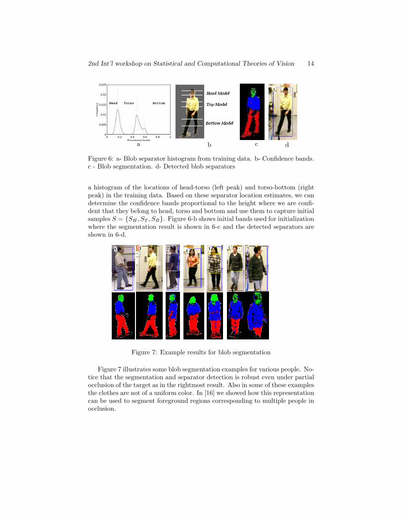
Figure 6: a- Blob separator histogram from training data. b- Confidence bands.c - Blob segmentation. d- Detected blob separators

a histogram of the locations of head-torso (left peak) and torso-bottom (rightpeak) in the training data. Based on these separator location estimates, we candetermine the confidence bands proportional to the height where we are confi-dent that they belong to head, torso and bottom and use them to capture initialsamples S = {SH , ST , SB}. Figure 6-b shows initial bands used for initializationwhere the segmentation result is shown in 6-c and the detected separators areshown in 6-d.

Figure 7: Example results for blob segmentation

Figure 7 illustrates some blob segmentation examples for various people. No-tice that the segmentation and separator detection is robust even under partialocclusion of the target as in the rightmost result. Also in some of these examplesthe clothes are not of a uniform color. In [16] we showed how this representationcan be used to segment foreground regions corresponding to multiple people inocclusion.


4 People Tracking Application

In this application we show how the fast Gauss transform algorithm can be usedto efficiently compute estimate for the gradient of the density as well as estimatefor the density itself. Estimation of density gradient is useful in applicationsthat use the mean shift algorithm [17, 18, 19, 20]. We utilize the color-spatialjoint distribution of a region as a constraint that is used to locate that regionin subsequent frames and therefore to track this region. The color-spatial jointdensity is estimated using kernel density estimation. An estimate of the gradientof the joint density is used to drive a gradient based search that is used to trackthat region. In order to reduce the dimensionality of the problem, we use onespatial dimension and two color dimensions to represent the joint color-spatialdensity. This is justified, since for the majority of clothing for people in uprightpose, the color distribution is independent of the horizontal axis and dependsonly on the vertical axis. That is, we are most likely to observe the same colordistribution orthogonal to the vertical axis. (Note that this does not assumeconstant horizontal color). This allows us to use only the vertical dimension inour representation of the joint color-spatial density. The independence of thecolor distribution from the abscissa makes the representation robust to rotationin depth.

Let S = {Xi}i=1..n be a set of sample pixels from the target region sothat Xi = (xi, yi, ui) where xi, yi is the sample pixel location around an origino, and ui ∈ Rd is a d-dimensional color vector. Given the sample S as amodel for the target region, the joint spatial-color probability of observing apixel X at location (x, y) with color u can be expressed as two independentdensity functions (since the color distribution is assumed to be independent ofthe horizontal axis and depends only on the vertical axis)

P (x, y, u) = F (x)H(y, u), (11)

where H(y, u) represents the joint density between the vertical location andthe color features and F (x) represents the distribution along the horizontalaxis. If we use two chromaticity variables u = (u1, u2) with diagonal covariancematrix to represent the color for each pixel, then we can estimate joint densityH(y, u | S) as:

H(y, u) =1N

N∑i=1

Kσy(y − yi)Kσu1(u1 − ui1)Kσu2

(u2 − ui2),

where σy, σu1 , σu2 are the kernel bandwidths in the three dimensions. Given atranslation of the region origin to a location (xc, yc) and a scaling hc, we canestimate the probability of a pixel X = (x, y, u) coming from S by shifting andscaling as

H(yc,hc)(y, u) =1N

N∑i=1

Kσy

(y − yc

hc− yi

)Kσu1

(u1 − ui1)Kσu2(u2 − ui2). (12)


Let R(c) be a region that represents the target with respect to a locationand a scaling hypothesis c = (xc, yc, hc), we define the likelihood function ψ(c)by integrating log probabilities over R as:

ψ(c) =∫

R

wc(x, y)L(Pc(x, y, u))dx (13)

where Pc(x, y, u) is an estimate of the joint density in 11, L(·) is a log functionand wc(x, y) is a weight kernel. Practically, we can assign more weights to pixelinside the region and less weights for pixels on the region boundary since theirinclusion in R is expected to be noisy. The target localization at frame t can beformalized as a search for a 2-D translation and a scaling that maximizes ψ(c).i.e., the location and scale hypothesis c = (xc, yc, hc) that maximizes ψ(c):

c = argc maxψ(c)

Given the joint density in equation 11 the likelihood function can be written as

ψ(c) =∑

(x,y,u)∈R

wc(x, y)L(Fc(x)) + wc(x, y)L(Hc(y, u))

We can drop the first term since this will be the same for all hypotheses, andso we can redefine ψ(.) in a simpler way as

ψ(c) =∑

(x,y,u)∈R

wc(x, y)L(Hc(y, u)) (14)

For the weights wc(x, y), we use Gaussian kernels N(xc, αxhc), N(yc, αyhc)where αx, αy are scaling constants in the horizontal and vertical direction.

0

50

100

150

200

250

300

350

0

50

100

150

200

2500

2

4

6

8

a) original image b) plot of surface ψ(c)

Figure 8: Likelihood function surface

The optimal target hypothesis represents a local maxima in the discrete threedimension search space. The log likelihood function is continuous and differen-tiable and, therefore, a gradient based optimization technique would convergeto that solution as long as the initial guess is within a small neighborhood ofthat maxima. Figure 8 shows a plot of the function ψ(c) for each location in


the image as a hypothesis for the target origin. For this plot, R was defined asa vertical ellipse of the same size as the target.

The derivation of the gradient of the objective function yields (after somemanipulation):

(αxh)2 · ∇xψ(c)ψ(c)

=

∑(x,y) xwc(x, y)L(Hc)∑(x,y)wc(x, y)L(Hc)

− xc

(αyh)2 · ∇yψ(c)ψ(c)

=

(αyh)2

∑(x,y)wc(x, y)

∇yHc

Hc∑(x,y)wc(x, y)L(Hc)

+

∑(x,y) ywc(x, y)L(Hc)∑(x,y)wc(x, y)L(Hc)

)− yc

where the term ∇yHc

Hcis the normalized gradient of the joint density Hc which

can be derived from equation 12 and can be expressed as

∇yHc(x, y, u)Hc(x, y, u)

=−1σ2h

· (15)

(∑Ni=1 xiKσy(y−yc

hc− yi)Kσu1

(u1 − ui1)Kσu2(u2 − ui2)∑N

i=1Kσy(y−yc

hc− yi)Kσu1

(u1 − ui1)Kσu2(u2 − ui2)

− y − yc

hc

)

The main computation overhead is the calculation of the joint density esti-mate Hc(y, u1, u2) and its gradient, ∇yHc(x, y, u). That is, the evaluation ofGaussian summation

S1(y, u1, u2) = C1

N∑i=1

e− 1

2 (y−yi

σy)2e− 1

2 (u1−ui1

σu1)2

e− 1

2 (u2−ui2

σu2)2

and a weighted version of it

S2(y, u1, u2) = C2

N∑i=1

yie− 1

2 (y−yi

σy)2e− 1

2 (u1−ui1

σu1)2

e− 1

2 (u2−ui2

σu2)2

Where C1,C2 are normalization constants and N is the number of samples inthe target model. At each iteration We need to evaluate these sums at eachpixel (x, y, u1, u2) in the region defined by each new region origin hypothesisc = (xc, yc, hc) where y = y−yc

hc. These summation is evaluated using Fast

Gauss algorithm where the sources are the sample points (yi, ui1, ui2)i=1..n andthe targets are the evaluation pixels (y, u1, u2) in candidate region R(c). Noticethat in the second summation each source is assigned a strength yi/

∑Ni=1 yi

To achieve efficient implementation, we developed a two phase version of thefast Gauss algorithm where in the first phase all the source data structures andexpansions are calculated from the samples. Then, at each new frame, these


Figure 9: Tracking result

structures and expansions are reused to evaluate the new targets. Since targets(evaluation points) are expected to be similar from frame to frame, the results ofeach evaluation are kept in a look up table to avoid doing repeated computation.

Figure 9 shows four frames from the tracking result for a sequence. Thesequence contains 40 frames taken at about 5 frames per second rate. Thetracker successfully locate the target at this low frame rate. Notice that thetarget changes his orientation during the tracking. Figure 10-left shows theperformance of the tracker on this sequence using Fast Gauss only (no look uptables). The average run-time per frame is about 200-300 msec. Figure 10-rightshows the performance of the tracker with look up tables used in conjunctionwith fast Gauss transform to save repeated computation. In this case, the runtime decreases with time and the average run time per frame is less than 20msec. This is more than 10 times speed up per iteration.

Figure 11 shows examples of tracking under partial occlusion. The target inthis case is waiting for the elevator and is not moving significantly. The resultsshows that the tracker continued to locate the target successfully throughoutseveral significant occlusion situation. Notice also that the horizontal location ofthe located region is not affected if some parts of the body are occluded. Sincethere is no significant motion in most of these sequence, motion based trackingwould fail in such a sequence. Also algorithms based on adaptive backgroundsubtraction might adapt to the target. Figure 12 shows results of tracking aperson in a crowd. These results are for videos captured at 10-12 frame persecond. The tracker successfully locates the targets at this low frame rate. Thebandwidths for the joint distribution kernels were set to 5%, 1%, 1% of eachdimension space size for σy,σu1 and σu1 respectively. The weight kernel w isnarrow in the horizontal direction (αx = 0.5 · width

2 ) and wide in the vertical

direction (αy = 1.8 · height2 ). Figure 13 shows a plot of the number of iterations


0 10 20 30 400

5

10

15

Frame

itera

tions

Number of iterations

0 10 20 30 400

100200300400500600

Frame

mse

c

Time for fast gauss evaluation per frame

0 10 20 30 4020304050607080

Frame

mse

c

Time for fast gauss evaluation per iteration

0 10 20 30 400

5

10

15

Frame

itera

tions

Number of iterations

0 10 20 30 400

102030405060

Frame

mse

c

Time for fast gauss evaluation per frame− with results LUT

0 10 20 30 4005

10152025303540

Frame

mse

c

Time for fast gauss evaluation per iteration − with results LUT

Figure 10: Performance of the tracker using Fast Gauss. Top: number of iter-ations per frame. Middle:run time per frame. Bottom: run time per iteration.Right: Performance using FGT with results look up tables.

needed for convergence for the sequence shown in figure 12.

5 Conclusion

In this paper we investigate the use of Fast Gauss Transform to speedup kerneldensity estimation techniques. We presented the use of kernel density estimationin modeling the color of homogeneous regions and used this modeling approachto segment foreground region corresponding to people into major body partsbased on color. We also presented the use of kernel estimation of the joint color-spatial density in tracking people. The tracking algorithm is robust to partialocclusion and rotation in depth. It can be used from moving or stationaryplatforms. In both applications, the FGT was used to efficiently compute thekernel density estimation and the gradient of the density, resulting in real-timeperformance. The Fast Gauss transform can be useful to many vision problemsthat use kernel density estimation, and as such our paper serves to introducethe algorithm to this community. Kernel density estimation is a better way toestimate the densities in comparison with classical parametric methods in caseswhere the underlying distribution are not known or when it is hard to specifythe right model. Also kernel density estimation is better than use of histogramtechniques, since a smooth and continuous estimate of the density is obtained,and the method has significantly improved memory complexity. The version of


Figure 11: Tracking under partial occlusion

the FGT algorithm that we presented here is a generalization of the originalalgorithm as it uses a diagonal covariance matrix instead of a scalar variance.Similar generalizations to the variable scale case will be reported elsewhere.


Figure 12: Tracking person in a crowd

1680 1720 1760 1800 18400

2

4

6

8

10

12

14

Frames

Itera

tion

Figure 13: Number of iterations for convergence


References

[1] R. O. Duda, D. G. Stork, and P. E. Hart, Pattern Classification. Wiley,John & Sons,, 2000.

[2] D. W. Scott, Mulivariate Density Estimation. Wiley-Interscience, 1992.

[3] L. Greengard, The Rapid Evaluation of Potential Fields in Particle Sys-tems. Cambridge, MA: MIT Press, 1988.

[4] L. Greengard and J. Strain, “The fast gauss transform,” SIAM J. Sci.Comput., 2, pp. 79–94, 1991.

[5] A. Ware, “Fast approximate fourier transforms for irregularly spaced data,”SIAM Review, vol. 40, pp. 838–856, December 1998.

[6] C. Lambert, S. Harrington, C. Harvey, and A. Glodjo, “Efficient on-linenonparametric kernel density estimation,” Algorithmica, no. 25, pp. 37–57,1999.

[7] J. Strain, “The fast gauss transform with variable scales,” SIAM J. Sci.Comput., vol. 12, pp. 1131–1139, 1991.

[8] “Approximate math library for intel streaming simd extensions, release2.0.” October 2000 Documentation File, Intel Corporation.

[9] J. Fritsch and I. Rogina, “The bucket box intersection (bbi) algorithm forfast approximative evaluation of diagonal mixture gaussians,” in Procedingsof the ICASSP 96, May 2-5, Atlanta, Georgia USA, 1996.

[10] C. R. Wern, A. Azarbayejani, T. Darrell, and A. P. Pentland, “Pfinder:Real-time tracking of human body,” IEEE Transaction on Pattern Analysisand Machine Intelligence, 1997.

[11] Y. Raja, S. J. Mckenna, and S. Gong, “Colour model selection and adapta-tion in dynamic scenes,” in 5th European Conference of Computer Vision,1998.

[12] Y. Raja, S. J. Mckenna, and S. Gong, “Tracking colour objects using adap-tive mixture models,” Image Vision Computing, no. 17, pp. 225–231, 1999.

[13] S. J. McKenna, S. Jabri, Z. Duric, and A. Rosenfeld, “Tracking groups ofpeople,” Computer Vision and Image Understanding, no. 80, pp. 42–56,2000.

[14] J. Martin, V. Devin, and J. Crowley, “Active hand tracking,” in IEEE In-ternational Conference on Automatic Face and Gesture Recognition, 1998.

[15] A. Elgammal, D. Harwood, and L. S. Davis, “Nonparametric backgroundmodel for background subtraction,” in 6th European Conference of Com-puter Vision, 2000.


[16] A. Elgammal and L. S. Davis, “Probabilistic framework for segmenting peo-ple under occlusion,” in 8th IEEE International Conference on ComputerVision, 2001.

[17] Y. Cheng, “Mean shift, mode seeking, and clustering,” IEEE Transactionon Pattern Analysis and Machine Intelligence, vol. 17, pp. 790–799, Aug1995.

[18] Y. Cheng and K. Fu, “Conceptual clustering in knowledge organization,”IEEE Transaction on Pattern Analysis and Machine Intelligence, vol. 7,pp. 592–598, 1985.

[19] D. Comaniciu, V. Ramesh, and P. Meer, “Real-time tracking of non-rigidobjects using mean shift,” in IEEE Conference on Computer Vision andPattern Recognition, vol. 2, pp. 142–149, Jun 2000.

[20] D. Comaniciu and P. Meer, “Mean shift analysis and applications,” in IEEE7th International Conference on Computer Vision, vol. 2, pp. 1197–1203,Sep 1999.

eﬃcient kernel density estimation using the fast gauss...

Documents