1

Identification with Conditioning Instruments in Causal Systems

Karim Chalak1 Halbert White Department of Economics Department of Economics Boston College University of California, San Diego

May 17, 2007

Abstract: We study the structural identification of causal effects with conditioning instruments within the settable system framework. In particular, we provide causal and predictive conditions sufficient for conditional exogeneity to hold. We provide two procedures based on “exclusive of A” (~A)-causality matrices and the direct causality matrix for inferring conditional causal isolation among vectors of settable variables and consequently conditional independence among corresponding vectors of random variables. Similarly, we provide sufficient conditions for conditional stochastic isolation in terms of the σ-algebras generated by the conditioning variables. We build on these results to study the structural identification of average effects and average marginal effects with conditioning instruments. We distinguish between structural proxies and predictive proxies. Acknowledgment: The authors thank Julian Betts, Graham Elliott, Clive Granger, Mark Machina, Dimitris Politis, and Ruth Williams for their helpful comments and suggestions. All errors and omissions are the authors’ responsibility.

1 Karim Chalak, Department of Economics, Boston College, 140 Commonwealth Avenue, Chestnut Hill, MA 02467 (email: chalak@bc.edu). Halbert White, Department of Economics 0508, University of California, San Diego, 9500 Gilman Drive, La Jolla, CA 92093-0508 (email: hwhite@ucsd.edu).

2

1. Introduction Researchers are often interested in measuring causal relationships and evaluating the effects of policies and interventions. In observational studies, this is a particularly challenging task for several reasons, including, among others, the inability of the researcher to control relevant variables, the fact that some relevant causes may be unobserved, and the unknown forms of response functions. White and Chalak (2006) (WC) discuss the role that conditional exogeneity can play in permitting informative causal inference in such situations. We employ WC’s settable system framework to study the specification of proxies that can function as conditioning instruments, as discussed in WC and Chalak and White (2007a), to support the structural identification of causal effects of interest. In particular, we build on results of Chalak and White (2007b) (CW) to provide causal and predictive conditions sufficient for conditional exogeneity to hold. In the nomenclature of the treatment effect literature, conditional exogeneity implies the property of “ignorability” or “unconfoundedness” (see e.g. Rubin, 1974; Rosenbaum and Rubin, 1983). Nevertheless, the treatment effect literature is typically silent as to how to construct valid covariates that ensure conditional exogeneity in observational studies. In standard experimental settings, the researcher may be able to control the assignment mechanism of the treatment, collect pre-treatment measurements, and perform diagnostic tests to ensure that conditional exogeneity holds (see e.g. Rosenbaum, 2002). For example, randomization or conditional randomization may be sufficient for useful causal inference (see WC). In such circumstances, the determination of suitable covariates is typically straightforward. On the other hand, in observational studies and certain experimental settings, such privileges are typically not available, and the researcher has to resort to alternative means for identification of effects of interest. In particular, economic theory can play a central role in providing guidance for constructing conditioning instruments that ensure conditional exogeneity and thus support the structural identification of causal effects of interest. A main goal of the present analysis is to examine in detail how information provided by underlying economic (or other) theory can be used to generate valid conditioning instruments, thereby identifying causal effects of interest in observational settings. We proceed with our analysis of structural identification with conditioning instruments under minimal assumptions. In econometrics, assumptions that may permit structural inference are typically concerned with the distribution of the unobserved variables or the functional form of the response functions or both (see e.g. Heckman and Robb, 1985; Heckman and Honore, 1990; Blundell and Powell, 2003; Matzkin, 2003; Heckman and Vytlacil, 2005). Here we impose only the weakest possible assumptions on the distribution of the unobserved variables and the functional form of the response functions. This extends the analysis of Chalak and White (2007a), who study in detail the identification of causal effects within the structural equations framework under the classic assumption of linearity. Their analysis reveals several extension of the concept of instrumental variables.

3

In brief, the main contribution of this paper is to provide formal and general causal and predictive conditions ensuring that conditional exogeneity holds, thus permitting informative causal inference. Our hope is that once these conditions have been properly justified by economic theory and expert knowledge, they can serve as helpful templates to guide empirical researchers in forming causal inferences. The paper is organized as follows. In Section 2, we build on results of CW to study conditioning instruments that ensure conditional exogeneity in a canonical recursive settable system, S. In Section 2.1, we define the direct causality matrix ( )dC S and, for a given set of causal variables whose indexes belong to a set A, the “exclusive of A” (~A)-causality matrix ~ ACS . We then provide two procedures for verifying the presence of structural proxies using ~ ACS and ( )dC S . These procedures rely on the fact that conditional independence holds by conditioning on the common causes of the variables of interest or on variables that fully mediate the effects of these common causes. This includes as a special case the notion of d-separation introduced in the artificial intelligence literature (see e.g. Pearl, 2000, p.16-17). Section 2.2 studies another special case of conditioning instruments that we refer to as predictive proxies, following WC and Chalak and White (2007a). In this case, conditional independence can hold due to a particular predictive relationship that holds among the variables of interest. Section 3 builds on results of WC to provide fully structural conditions ensuring that conditioning instruments permit the structural identification of covariate-conditioned average effects and covariate-conditioned average marginal ceteris paribus effect. The structural identification results in Section 3 that employ structural proxies include as a special case methods based on the “back door criterion” introduced in the artificial intelligence literature by Pearl (1995, 2000). We are not aware of results that study structural identification with predictive proxies other than the results of WC and Chalak and White (2007a). Section 4 concludes and discusses directions for future research. Formal mathematical proofs are collected into the Mathematical Appendix. 2. Conditioning Instruments in Settable Systems We work with the version of settable systems presented in definition 2.1 of CW. Specifically, we consider canonical recursive settable systems S ≡ (Ω, F), (Z, Π, rΠ ,

X) (CW definition 2.6). A settable system has a stochastic component, (Ω, F), and a

structural component, (Z, Π, rΠ , X). WC provide a detailed discussion. A settable system S represents agents indexed by h = 1, 2…, each governing settable variables indexed by j

= 1, 2, …, represented as Xh ≡ Xh,j, where Xh,j: 0,1 × Ω → R. A special settable

variable, the fundamental settable variable, is denoted X0. Settable variables X ≡ Xh generate settings Z = Zh,j = Xh,j(1, . ) and, for the given partition Π ≡ Πb, responses Y = Yh,j = Xh,j(0, . ), given by Yh,j = ,h jrΠ (Z(b)) for (h, j) in Πb, h ≠ 0, where ,h jrΠ is the response function, and Z(b) denotes settings of variables not belonging to partition block

4

Πb. By convention, Π0 = 0. In recursive settable systems, the blocks are ordered such that responses in higher-level blocks depend only on settings in lower-level blocks. In canonical recursive settable systems, we further have Zh,j = Yh,j for h ≠ 0. By convention, we also have Z0 = Y0. For simplicity, we sometimes consider finite settable systems, that is, systems with a finite number of agents and responses so that j = 1, …, Jh, with Jh < ∞ , h = 1, …, H < ∞ . 2.1 Causally Isolating Conditioning Instruments Next, we provide definitions of certain matrices that summarize aspects of interest associated with settable systems. We make use of these definitions shortly for inspecting conditional independence relationships.

Following CW, we write Xh,j d

S⇒ Xi,k when Xh,j directly causes Xi,k in S and we write

Xh,j |d

S⇒ Xi,k otherwise (see CW, definition 2.3). For a settable system S, we define the

direct causality matrix ( )dC S associated with S. Definition 2.1: Direct Causality Matrix Let S ≡ (Ω, F), (Z, Π, rΠ , X) be a finite

canonical recursive settable system. The direct causality matrix associated with S, denoted by ( )dC S , has elements given by:

( )( , ),( , )dh j i kc S = 1 if Xh,j

d

S⇒ Xi,k,

( )( , ),( , )dh j i kc S = 0 if Xh,j |

d

S⇒ Xi,k. Thus, ( )dC S has the form:

X0 (0, ·) X1,1 (0, ·) … , HH JX (0, ·)

X0 (1, ·) 0

X1,1 (1, ·) 0 0

( )dC S =

, HH JX (1, ·) 0 0 We note some properties of ( )dC S . The diagonal entries are ( )

( , ),( , )dh j h jc S = 0 for j = 1, …, Jh,

h = 1, …, H, since Xh,j |d

S⇒ Xh,j by definition. Also, the entries of the first column ( )( , ),0dh jc S

= 0 for j = 1, …, Jh, h = 1, …, H, since Xh,j |d

S⇒ X0 by definition. Blank entries of ( )dC S

5

can take the values 0 or 1. Let G = (V, E) be the directed graph associated with S, where V = Xh,j : j = 1, …, Jh; h = 0, 1, …, H is a non-empty finite set of vertices and E ⊂ V ×V

is a set of arcs such that an arc (Xh,j, Xi,k) belongs to E if and only if Xh,j

d

S⇒ Xi,k. Since S is recursive, G admits an acyclic ordering of its vertices. Bang-Jensen and Gutin’s (2001 p. 175) DFSA algorithm outputs an acyclic ordering of the vertices of G. It follows that

there exists a 1

H

hh

J=

∑ × 1

H

hh

J=

∑ permutation matrix ( )dM S such that ( )dM S × ( )dC S is

strictly upper triangular. The recursiveness of S further imposes the following constraints on ( )dC S : Proposition 2.2: Acyclicality Let S ≡ (Ω, F), (Z, Π, rΠ , X) be a finite canonical

recursive settable system and let ( )dC S be the direct causality matrix associated with S. Then, for all sets of n distinct elements, say (h1, j1), …, (hn, jn), of 0, (1,1), …, (H,

JH) with 1 ≤ n ≤ 1

H

hh

J=

∑ we have:

1 1 2 2 2 2 3 3 1 1

( ) ( ) ( )( , ),( , ) ( , ),( , ) ( , ),( , )...

n n

d d dh j h j h j h j h j h jc c c× ×S S S = 0.

Similarly, for a set A of index pairs, we define the causality matrix exclusive of A (or ~A-causality matrix) ~ ACS associated with a recursive settable system S. Following CW, we let ( , ):( , )h j i kI denote the set of (Xh,j, Xi,k) d(S)-intercessors and we let ind( ( , ):( , )h j i kI ) denote

the set of indexes of the elements of ( , ):( , )h j i kI . For A ⊂ ind( ( , ):( , )h j i kI ), we write Xh,j ~A

S⇒

Xi,k when Xh,j causes Xi,k exclusive of XA (or Xh,j ~A-causes Xi,k) with respect to S. We write Π0 ≡ 0. Definition 2.2: Causality Matrix Exclusive of A (~A-Causality Matrix) Let S ≡ (Ω,

F), (Z, Π, rΠ , X) be a finite canonical recursive settable system. For given non-negative

integers b1 and b2, let (h, j) ∈ 1bΠ , and let (i, k) ∈

2bΠ . Let A ⊂ Π ∪ Π0, and let

( , ):( , )h j i kA = A ∩ ind( ( , ):( , )h j i kI ). The ~A-causality matrix associated with S denoted by

~ ACS has elements given by:

,~( , ),( , )

Ah j i kcS = 1 if b1 < b2, (h, j), (i, k) ∉ A, and Xh,j

( , ):( , )~ h j i kA

S⇒ Xi,k, ,~

( , ),( , )A

h j i kcS = 0 otherwise.

6

~ ACS and ( )dC S share similar properties. In particular, ,~( , ),( , )

Ah j h jcS = ,~

( , ),0A

h jcS = 0 for j = 1, …, Jh, h = 1, …, H by definition. Similarly, since there exists a non-recursive ordering of the

sequence Πb, it follows that there exists a 1

H

hh

J=

∑ × 1

H

hh

J=

∑ permutation matrix M S

such that M S × ~ ACS is strictly upper triangular. When A = ∅ , we refer to the ~∅ -causality matrix simply as the causality matrix, denoted by CS . Let A and B be nonempty disjoint subsets of Π ∪ Π0, and denote by XA and XB the corresponding vectors of settable variables. Following CW, we denote by :A BI ≡

( , )h j A∈∪ ( , )i k B∈∪ ( , ):( , )h j i kI \ (XA ∪ XB) the set of (XA, XB) d(S)-intercessors and we let ind( :A BI ) denote the set of indexes of the elements of :A BI . Also, we adopt CW’s definitions of direct, indirect, and A-causality for vectors of settable variables. In

particular, for C ⊂ ind( :A BI ), we write XA ~C

S⇒ XB when XA causes XB exclusive of XC (i.e., XA ~C-causes XB) with respect to S. Theorem 4.6 of CW provides necessary and sufficient conditions for stochastic conditional dependence among certain random vectors in settable systems. In particular, it follows from this result that if XA and XB are conditionally causally isolated given XC, then their corresponding random vectors YA and YB are conditionally independent given YC. Our next proposition demonstrates that XC-conditional causal isolation and thus certain conditional independence relationships can be immediately verified by inspecting the ~C-causality matrix, ~CCS . For this, we let a = maxb: there exists (h, j) ∈ bΠ ∩ A and b = maxb: there exists (i, k) ∈ bΠ ∩ B. As in CW, for any blocks a, b, 0 ≤ a ≤ b, we let [ : ]a bΠ ≡ 1...a b b−Π Π Π∪ ∪ ∪ . Proposition 2.3 Let S ≡ (Ω, F, P), (Z, Π, rΠ , X) be a finite canonical settable system.

Let A and B be nonempty disjoint subsets of Π ∪ Π0, and let XA and XB be corresponding vectors of settable variables. Let C ⊂ 1:[max( , ) 1]a b −∏ \ (A ∪ B), let XC be the

corresponding vector of settable variables, and let ~CCS be the ~C-causality matrix associated with S. Let YA = XA (0, . ), YB = XB (0, . ), and YC = XC (0, . ). Then (a) XA and XB are conditionally causally isolated given XC if and only if (i) 0 ∈ A and ,~

0,( , )C

i kcS = 0 for all (i, k) ∈ B; or

(ii) 0 ∈ B and ,~0,( , )

Ch jcS = 0 for all (h, j) ∈ A; or

(iii) 0 ∉ A ∪ B and ,~0,( , )

Ch jcS = 0 for all (h, j) ∈ A or ,~

0,( , )C

i kcS = 0 for all (i, k) ∈ B.

7

(b) Suppose that either (a.i), (a.ii), or (a.iii) hold; then for every probability measure P on (Ω, F), YA ⊥ YB | YC.

A practical benefit of this result is that it can be straightforwardly converted into a computer algorithm that can be used to verify conditional causal isolation, and thus conditional independence, for any triple YA, YB, YC. Note, however, that the failure to verify conditional causal isolation does not imply conditional dependence. We discuss this further below. As discussed in CW, determining ~A-causality relationships among settable variables generally requires knowledge of the functional form of the response functions associated with the settable variables under study. In economics and other fields where observational studies predominate, it is often true that the researcher does not have detailed information about the functional form of the response functions. Frequently, the researcher may know only whether or not a given variable is a direct cause of another. Is it possible to deduce conditional independence from knowledge only of a direct causality matrix? Our next results demonstrate that the answer to this question is indeed positive. For brevity, we may drop explicit reference to d(S) in what follows when referring to

( )( , ),( , )dh j i kc S , as well as the matrices that obtain from ( )dC S and their entries. For example, we

write c(h,j),(i,k) to denote an element of ( )dC S . Definition 2.4: Path Conditional Matrix given XA Let S ≡ (Ω, F), (Z, Π, rΠ , X) be a

finite canonical settable system. Let A ⊂ Π ∪ Π0 and let XA be the corresponding vector of settable variables. The path conditional matrix given XA, denoted AP , is given by AP =

Ap ( ( )dC S ) where the elements of Ap (·) are defined as:

( , ),( , )Ah j i kp = 1 if (h, j), (i, k) ∉ A, and ( , ),( , )h j i kc = 1 or there exists a subset

(h1, j1), …, (hn, jn) of Π \ A with 1 ≤ n ≤ 1

H

hh

J=

∑ such that

1 1 1 1 2 2( , ),( , ) ( , ),( , ) ( , ),( , )... 1

n nh j h j h j h j h j i kc c c× × × = , ( , ),( , )

Ah j i kp = 0 otherwise.

Definition 2.4 can be conveniently visualized using the graph G associated with S. In fact, ( , ),( , )

Ah j i kp = 1 if and only if there exists in G an (Xh,j, Xi,k)-path of positive length that

does not contain elements of A.

8

Our next result demonstrates that it is possible to verify certain ~A-causality relationships from knowledge of only ( )dC S , and thus AP , without further information on the functional form of the response functions. Lemma 2.5 Let S, XA, XB and XC be as in Proposition 2.3. Let CP be the direct path conditional matrix given CX . Let CA:B = C ∩ ind( :A BI ). Suppose that ( , ),( , )

Ch j i kp = 0 for

all (h, j) ∈ A and (i, k) ∈ B. Then XA :~

|ABC

S⇒ XB. We now provide sufficient conditions for the conditional independence of certain random vectors in settable systems expressed in terms of ( )dC S . Corollary 2.6 Let S, XA, XB, XC be as Proposition 2.3, and let CP be the path conditional matrix given CX . Let YA = XA (0, . ), YB = XB (0, . ), and YC = XC (0, . ). Suppose that either (i) 0 ∈ A and 0,( , )

Ci kp = 0 for all (i, k) ∈ B; or

(ii) 0 ∈ B and 0,( , )C

h jp = 0 for all (h, j) ∈ A; or

(iii) 0 ∉ A ∪ B and 0,( , )C

h jp = 0 for all (h, j) ∈ A or 0,( , )C

i kp = 0 for all (i, k) ∈ B. Then XA and XB are conditionally causally isolated given XC and for every probability

measure P on (Ω, F), YA ⊥ YB | YC.

The graph G associated with a system S can play a particularly helpful role in verifying conditional independence via Corollary 2.6. In fact, when 0 ∉ A, if, for all (h, j) ∈ A, there does not exist a (X0, Xh,j)-path that does not contain elements of C then YA ⊥ YB | YC. A parallel result holds when 0 ∉ B. When further assumptions are imposed on the probability measure P, Corollary 2.6 include as a special case the notion of d-separation discussed in the artificial intelligence literature (see Pearl 2000, p. 16-17, 68-69; and CW section 5). As is true for Proposition 2.3, Corollary 2.6 provides the basis for a straightforward computer algorithm that can be used to verify conditional causal isolation, and thus conditional independence. Corollary 2.6 provides sufficient but not necessary conditions for conditional

independence. In fact, it is possible to have XA :~

|ABC

S⇒ XB even when ( , ),( , )Ch j i kp = 1 for all (h,

j) ∈ A and (i, k) ∈ B, due to a cancellation of direct and indirect effects. Nevertheless, such inference requires detailed knowledge of the response functions. Thus, it is possible for XA and XB to be causally isolated given XC even when conditions (i), (ii), and (iii) of

9

Corollary 2.6 fail. For example, when A = (h, j) and B = (i, k) we may have 0,( , )C

h jp × 0,( , )C

i kp = 1 and Yh,j ⊥ Yi,k | YC. Pearl (2000, p. 48-49) and Spirtes et al (1993, p. 35, 56) introduce the assumptions of “stability” or “faithfulness” on P to ensure that the conditions in Proposition 2.3 and Corollary 2.6 deliver the same conclusion. Here, however, we see that it is the behavior of the response functions and not the properties of the probability measure that determine whether or not the conclusions of Proposition 2.3 and Corollary 2.6 coincide. When C = ∅ , we simply call PS the path matrix associated with S and Corollary 2.6 then provides conditions ensuring the stochastic independence of YA and YB. This result is, however, less interesting since the conditions of Corollary 2.6 imply that either YA or YB (or both) are constants (see CW, lemma 3.1). For given nonempty disjoint subsets A and B of Π ∪ Π0, one can ask what is the is the smallest set C ⊂ 1:[max( , ) 1]a b −∏ \ (A ∪ B) (if any) such that the realizations of YC = XC (0, .

) are observed and XC conditionally causally isolates XA and XB. In addition to supporting computer algorithms that can verify conditional causal isolation, Proposition 2.3 and Corollary 2.6 provide the basis for constructing algorithms that may output such a set C. We leave development of these algorithms to other work. Thus, Proposition 2.3 and Corollary 2.6 provide causal conditions sufficient to ensure that vectors of settable variables XA and XB are causally isolated given XC and thus that YA ⊥ YB | YC. This conditional independence holds because the common causes of XA and XB, or variables that fully mediate the effects of these common causes on either (or both) XA and XB, are elements of XC (see CW, section 5). In Section 3, we discuss how such a “causally isolating” XC can play an instrumental role in ensuring conditional exogeneity. In this case, we refer to XC and its settings ZC = YC as causally isolating conditioning instruments or structural proxies. 2.2 Stochastically Isolating Conditioning Instruments CW demonstrate that YA ⊥ YB | YC can also hold when XA and XB are not conditionally causally isolated given XC, provided that P stochastically isolates XA and XB given XC. We now study special cases in which this can happen. We build on results of Van Putten and Van Schuppen (1985), who study certain operations that leave conditional independence relationships invariant. In particular, we focus on operations that enlarge or reduce the conditioning σ-algebra and that preserve the conditional independence relationships of interest. First, we adapt definitions from Van Putten and Van Schuppen (1985) to our context.

10

Definition 2.7 Projection Operator for σ-Algebras Let S ≡ (Ω, F, P), (Z, Π, rΠ , X)

be a canonical recursive settable system. (i) Let F ≡ G ⊂ F | G is a σ-algebra that contains all the P-null sets of F.

(ii) If H, G ∈ F, then H∨ G is the smallest σ-algebra in F that contains H and G.

(iii) For G ∈ F, let L+(G) = g : Ω → + | g is G-measurable.

(iv) For H, G∈ F let the projection of H on G be the σ-algebra

σ(H | G) ≡ σ(E[h | G] | for all h ∈ L+(H)) ∈ F,

with the understanding that the P-null sets of F are adjoined to it.

The next result helps to characterize situations where P is stochastically isolating. Theorem 2.8 Let S ≡ (Ω, F, P), (Z, Π, rΠ , X) be a canonical settable system. Let A

and B be nonempty disjoint subsets of Π ∪ Π0, and let XA and XB be corresponding vectors of settable variables. Let C1 and C2 be subsets of 1:[max( , ) 1]a b −∏ \ (A ∪ B) and let

1CX and 2CX denote the corresponding vectors of settable variables. Let YA = XA (0, . ), YB

= XB (0, . ), 1CY =

1CX (0, . ), and 2CY =

2CX (0, . ) generate σ-algebras A, B, C1, and C2 ∈

F such that C2 ⊂ C1. Then (a.i) 1CX causally isolates XA and XB or (a.ii) P stochastically

isolates XA and XB given 1CX and (b) σ(A | C1) ⊂ C2 if and only if (c.i)

2CX causally

isolates XA and XB or (c.ii) P stochastically isolates XA and XB given 2CX and (d) σ(A |

B∨ C1) ⊂ (B∨ C2).

When YA, YB, and

1CY are as in Theorem 2.8, theorem 4.6 in CW gives that YA ⊥ YB | 1CY

if and only if 1CX causally isolates XA and XB or P stochastically isolates XA and XB

given 1CX . Heuristically, one can view a σ-algebra A as representing information, A∨ B

as the smallest set containing the information in both A and B, and σ(A | C) as the

information about A inferred from the information in C. Similarly, one can understand YA

11

⊥ YB | YC as the statement that knowledge of information C renders information in A

irrelevant for information B (and thus the information in B irrelevant for information A). Now suppose that information C2 is a subset of information C1. Theorem 2.8 states that

(a) knowledge of C1 renders A irrelevant for B and (b) the information about A inferred

from C1 is a subset of C2 if and only if (c) knowledge of C2 renders A irrelevant for B

and (d) the information about A inferred from B and C1 is contained in information

B and C2. Thus, Theorem 2.8 provides necessary and sufficient conditions for preserving a conditional independence relationship among vectors of random variables YA and YB when the information that we condition on is either enlarged or reduced. Examples of this enlargement or reduction relevant here occur when we know that conditional independence holds when conditioning on unobservables, and we seek to find observables that we can condition on instead that will preserve conditional independence. Next, we state a helpful Corollary of Theorem 2.8. Corollary 2.9 Let S, XA, XB,

1CX , and 2CX be as in Theorem 2.8. Let YA = XA (0, . ), YB =

XB (0, . ), 1CY =

1CX (0, . ), and 2CY =

2CX (0, . ) generate σ-algebras A, B, C1, and C2 ∈ F.

Suppose that (a.i) 1CX causally isolates XA and XB or (a.ii) P stochastically isolates XA

and XB given 1CX and (b) σ(A | C1) ⊂ C2 ⊂ (B∨ C1). Then (c.i)

2CX causally isolates

XA and XB or (c.ii) P stochastically isolates XA and XB given 2CX .

Suppose that YA, YB,

1CY , and 2CY are as in Theorem 2.8 and that

1CX causally isolates XA

and XB or that P stochastically isolates XA and XB given 1CX , so that YA ⊥ YB |

1CY .

Heuristically, Corollary 2.9 states that if (a) knowledge of C1 renders A irrelevant for B,

(b.i) C2 contains the information about A inferred from C1, and (b.ii) C2 is contained in

B and C1, then (c) knowledge of C2 renders A irrelevant for B. In other words, (b.i) and

(b.ii) state that C2 contains the information in C1 relevant for A but does not contain

information not included in B and C1. Thus, Corollary 2.9 provides a bound on C2

sufficient for YA ⊥ YB | 2CY to hold.

If the conditions of Corollary 2.9 hold and if

2CX does not causally isolate XA and XB,

then it must be that P stochastically isolates XA and XB given 2CX . In this case, YA ⊥ YB |

12

2CY holds, but not because the common causes of XA and XB (or variables that fully

mediate the effects of these common causes on either (or both) XA and XB) are elements of

2CX . Instead, conditional independence holds because of a predictive relationship that relates YA, YB,

1CY , and 2CY , motivating our terminology designating

2CZ =2CY as

predictive proxies. Parallel to our nomenclature above, we may also call 2CZ =

2CY stochastically isolating conditioning instruments. Observe that in such situations YA ⊥ YB |

2CY , but that XA and XB are not d-separated given

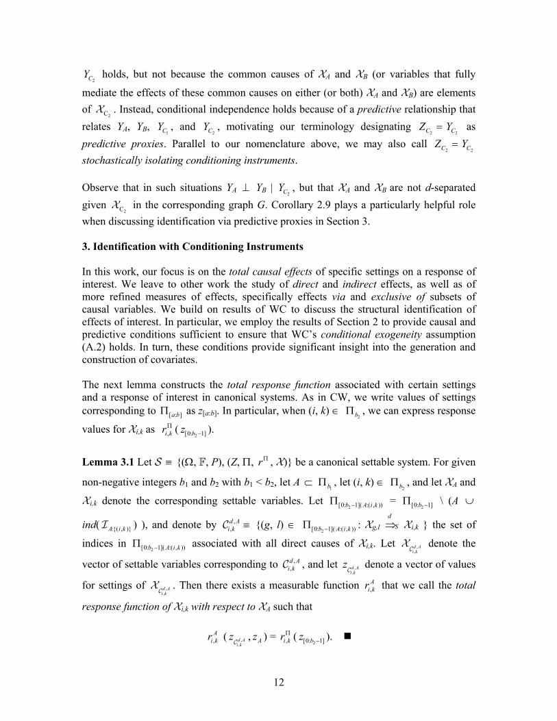
2CX in the corresponding graph G. Corollary 2.9 plays a particularly helpful role when discussing identification via predictive proxies in Section 3. 3. Identification with Conditioning Instruments In this work, our focus is on the total causal effects of specific settings on a response of interest. We leave to other work the study of direct and indirect effects, as well as of more refined measures of effects, specifically effects via and exclusive of subsets of causal variables. We build on results of WC to discuss the structural identification of effects of interest. In particular, we employ the results of Section 2 to provide causal and predictive conditions sufficient to ensure that WC’s conditional exogeneity assumption (A.2) holds. In turn, these conditions provide significant insight into the generation and construction of covariates. The next lemma constructs the total response function associated with certain settings and a response of interest in canonical systems. As in CW, we write values of settings corresponding to [ : ]a bΠ as z[a:b]. In particular, when (i, k) ∈

2bΠ , we can express response

values for Xi,k as ,i krΠ (2[0: 1]bz − ).

Lemma 3.1 Let S ≡ (Ω, F, P), (Z, Π, rΠ , X) be a canonical settable system. For given

non-negative integers b1 and b2 with b1 < b2, let A ⊂ 1bΠ , let (i, k) ∈

2bΠ , and let XA and

Xi,k denote the corresponding settable variables. Let 2[0: 1]( :( , ))b A i k−Π =

2[0: 1]b −Π \ (A ∪

ind( :( , )A i kI ) ), and denote by ,,d A

i kC ≡ (g, l) ∈ 2[0: 1]( :( , ))b A i k−Π : Xg,l

d

S⇒ Xi,k the set of

indices in 2[0: 1]( :( , ))b A i k−Π associated with all direct causes of Xi,k. Let ,

,d Ai kC

X denote the

vector of settable variables corresponding to ,,d A

i kC , and let ,,d Ai k

zC

denote a vector of values

for settings of ,,d Ai kC

X . Then there exists a measurable function ,A

i kr that we call the total

response function of Xi,k with respect to XA such that

,A

i kr ( ,,d Ai k

zC

, Az ) = ,i krΠ (2[0: 1]bz − ).

13

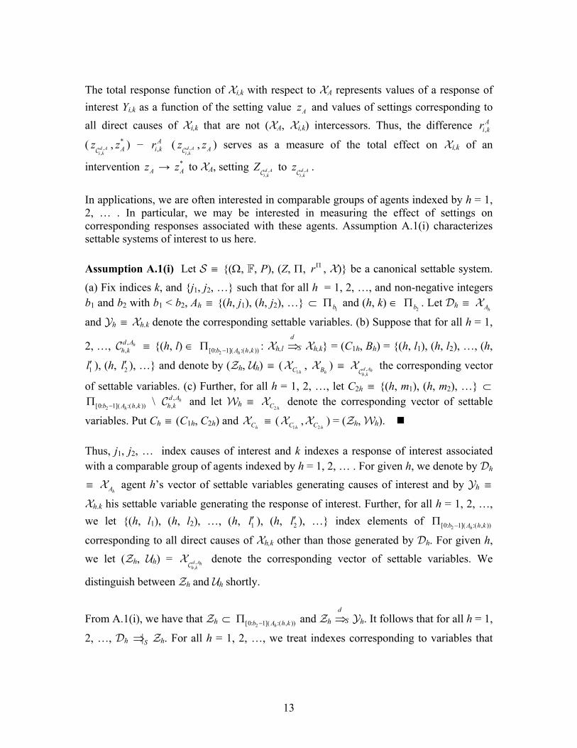
The total response function of Xi,k with respect to XA represents values of a response of interest Yi,k as a function of the setting value Az and values of settings corresponding to all direct causes of Xi,k that are not (XA, Xi,k) intercessors. Thus, the difference ,

Ai kr

( ,,d Ai k

zC

, *Az ) − ,

Ai kr ( ,

,d Ai k

zC

, Az ) serves as a measure of the total effect on Xi,k of an

intervention Az → *Az to XA, setting ,

,d Ai k

ZC

to ,,d Ai k

zC

.

In applications, we are often interested in comparable groups of agents indexed by h = 1, 2, … . In particular, we may be interested in measuring the effect of settings on corresponding responses associated with these agents. Assumption A.1(i) characterizes settable systems of interest to us here. Assumption A.1(i) Let S ≡ (Ω, F, P), (Z, Π, rΠ , X) be a canonical settable system. (a) Fix indices k, and j1, j2, … such that for all h = 1, 2, …, and non-negative integers b1 and b2 with b1 < b2, Ah ≡ (h, j1), (h, j2), … ⊂

1bΠ and (h, k) ∈ 2bΠ . Let Dh ≡

hAX

and Yh ≡ Xh.k denote the corresponding settable variables. (b) Suppose that for all h = 1,

2, …, ,,

hd Ah kC ≡ (h, l) ∈

2[0: 1]( :( , ))hb A h k−Π : Xh,l d

S⇒ Xh,k = (C1h, Bh) = (h, l1), (h, l2), …, (h,

1l′ ), (h, 2l′ ), … and denote by (Zh, Uh) ≡ (1hCX ,

hBX ) ≡ ,,

d Ahh kC

X the corresponding vector

of settable variables. (c) Further, for all h = 1, 2, …, let C2h ≡ (h, m1), (h, m2), … ⊂

2[0: 1]( :( , ))hb A h k−Π \ ,,

hd Ah kC and let Wh ≡

2 hCX denote the corresponding vector of settable

variables. Put Ch ≡ (C1h, C2h) and hCX ≡ (

1hCX ,2 hCX ) = (Zh, Wh).

Thus, j1, j2, … index causes of interest and k indexes a response of interest associated with a comparable group of agents indexed by h = 1, 2, … . For given h, we denote by Dh ≡

hAX agent h’s vector of settable variables generating causes of interest and by Yh ≡

Xh.k his settable variable generating the response of interest. Further, for all h = 1, 2, …, we let (h, l1), (h, l2), …, (h, 1l′ ), (h, 2l′ ), … index elements of

2[0: 1]( :( , ))hb A h k−Π

corresponding to all direct causes of Xh,k other than those generated by Dh. For given h, we let (Zh, Uh) = ,

,d Ahh kC

X denote the corresponding vector of settable variables. We

distinguish between Zh and Uh shortly.

From A.1(i), we have that Zh ⊂ 2[0: 1]( :( , ))hb A h k−Π and Zh

d

S⇒ Yh. It follows that for all h = 1,

2, …, Dh |S⇒ Zh. For all h = 1, 2, …, we treat indexes corresponding to variables that

14

succeed hAX but are not (

hAX , Xh,k) intercessors as elements of 2 2 1 ...b b +Π Π∪ ∪ without

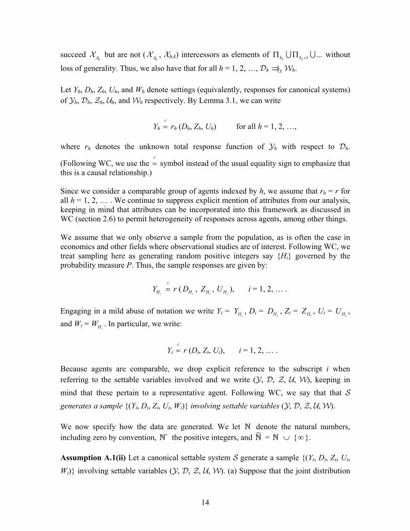
loss of generality. Thus, we also have that for all h = 1, 2, …, Dh |S⇒ Wh. Let Yh, Dh, Zh, Uh, and Wh denote settings (equivalently, responses for canonical systems) of Yh, Dh, Zh, Uh, and Wh respectively. By Lemma 3.1, we can write

Yh c= rh (Dh, Zh, Uh) for all h = 1, 2, …,

where rh denotes the unknown total response function of Yh with respect to Dh.

(Following WC, we use the c= symbol instead of the usual equality sign to emphasize that

this is a causal relationship.) Since we consider a comparable group of agents indexed by h, we assume that rh = r for all h = 1, 2, … . We continue to suppress explicit mention of attributes from our analysis, keeping in mind that attributes can be incorporated into this framework as discussed in WC (section 2.6) to permit heterogeneity of responses across agents, among other things. We assume that we only observe a sample from the population, as is often the case in economics and other fields where observational studies are of interest. Following WC, we treat sampling here as generating random positive integers say Hi governed by the probability measure P. Thus, the sample responses are given by:

iHY

c= r (

iHD , iHZ ,

iHU ), i = 1, 2, … . Engaging in a mild abuse of notation we write Yi =

iHY , Di = iHD , Zi =

iHZ , Ui = iHU ,

and Wi = iHW . In particular, we write:

Yi c= r (Di, Zi, Ui), i = 1, 2, … .

Because agents are comparable, we drop explicit reference to the subscript i when referring to the settable variables involved and we write (Y, D, Z, U, W), keeping in mind that these pertain to a representative agent. Following WC, we say that that S generates a sample (Yi, Di, Zi, Ui, Wi) involving settable variables (Y, D, Z, U, W). We now specify how the data are generated. We let N denote the natural numbers, including zero by convention, +N the positive integers, and N = N ∪ ∞ . Assumption A.1(ii) Let a canonical settable system S generate a sample (Yi, Di, Zi, Ui, Wi) involving settable variables (Y, D, Z, U, W). (a) Suppose that the joint distribution

15

of (Di, Xi) ≡ (Di, Zi, Wi) is H and the conditional distribution of Ui given (Di, Xi) = (d, x) is G( · | d, x) for all i = 1, 2, …, where Di is is 1k -valued, k1 ∈ +N , Zi is 2k -valued, k2 ∈ N , Ui is 4k -valued, k4 ∈ N , and Wi is 3k -valued, k3 ∈ N . (b) Let the responses Yi of Y be given by :

Yi c= r (Di, Zi, Ui), i = 1, 2, …,

where r denotes the unknown scalar-valued total response function of Y with respect to D. (c) We assume that the realizations of Yi, Di, Zi, and Wi are observed but that those of Ui are not. The identical distribution assumption A.1(a, b) is not necessary to our analysis but significantly simplifies our notation. We employ it in what follows to drop reference to the subscript i from the sample variables. Further, we let d, x ≡ (z, w), and u denote values of settings D, X ≡ (Z, W), and U respectively. With r the total response function of Y with respect to D, the total effect on Y of the intervention d → d* to D given Z = z and U = u, is r (d*, z, u) − r (d, z, u). Nevertheless, we cannot measure this difference, as the function r is not known. Further, even if r were known, the fact that the realizations of U are not observed prevents us from measuring the total effect on Y of an intervention d → d* to D. One accessible measurement is the conditional average response over the distribution of the unobserved variables given the observed variables. Following WC, we refer to X = (Z, W) as covariates. In fact, proposition 3.1 in WC shows that when E(Y) < ∞ , the average response given (D, X) = (d, x) exists, is finite, and for each (d, x) in supp(D, X) (the support of (D, X)), it is given by

µ (d, x) = ( , , ) ( | , )r d z u dG u d x∫ . The average response function µ is informative about the expected response given realizations (d, x) of (D, X). However, without further assumptions, it does not permit measurement of the total effect on Y of the intervention d → d* to D. When E(r(d, Z, U)) exists and is finite for each d in supp(D), WC define the average counterfactual response at d given X = x as

ρ (d, x) ≡ E (r(d, Z, U) | X = x) = ( , , ) ( | )r d z u dG u x∫ , where G( · | x) is the conditional distribution of U given X = x. WC show that under suitable assumptions, this conditional expectation has a clear counterfactual

16

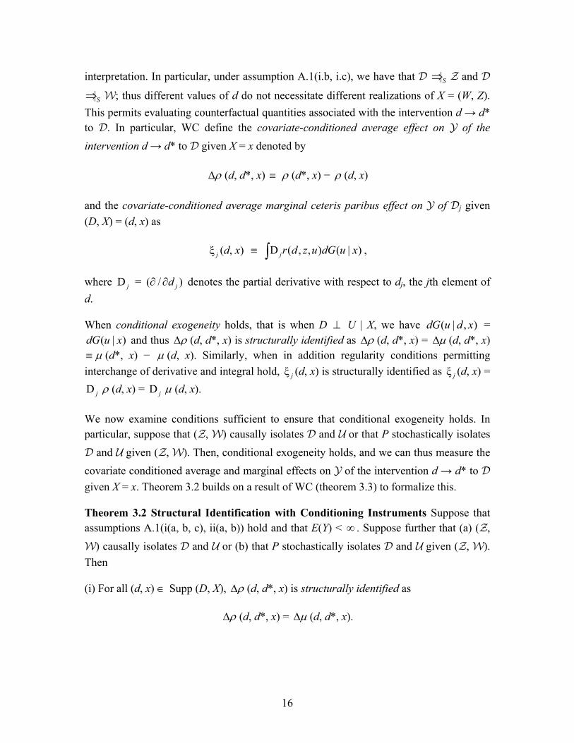
interpretation. In particular, under assumption A.1(i.b, i.c), we have that D |S⇒ Z and D

|S⇒ W; thus different values of d do not necessitate different realizations of X = (W, Z). This permits evaluating counterfactual quantities associated with the intervention d → d* to D. In particular, WC define the covariate-conditioned average effect on Y of the intervention d → d* to D given X = x denoted by

ρ∆ (d, d*, x) ≡ ρ (d*, x) − ρ (d, x) and the covariate-conditioned average marginal ceteris paribus effect on Y of Dj given (D, X) = (d, x) as

ξ j (d, x) ≡ D ( , , ) ( | )jr d z u dG u x∫ ,

where D j = ( / )jd∂ ∂ denotes the partial derivative with respect to dj, the jth element of d. When conditional exogeneity holds, that is when D ⊥ U | X, we have ( | , )dG u d x =

( | )dG u x and thus ρ∆ (d, d*, x) is structurally identified as ρ∆ (d, d*, x) = µ∆ (d, d*, x) ≡ µ (d*, x) − µ (d, x). Similarly, when in addition regularity conditions permitting interchange of derivative and integral hold, ξ j (d, x) is structurally identified as ξ j (d, x) = D j ρ (d, x) = D j µ (d, x). We now examine conditions sufficient to ensure that conditional exogeneity holds. In particular, suppose that (Z, W) causally isolates D and U or that P stochastically isolates D and U given (Z, W). Then, conditional exogeneity holds, and we can thus measure the covariate conditioned average and marginal effects on Y of the intervention d → d* to D given X = x. Theorem 3.2 builds on a result of WC (theorem 3.3) to formalize this. Theorem 3.2 Structural Identification with Conditioning Instruments Suppose that assumptions A.1(i(a, b, c), ii(a, b)) hold and that E(Y) < ∞ . Suppose further that (a) (Z, W) causally isolates D and U or (b) that P stochastically isolates D and U given (Z, W). Then (i) For all (d, x) ∈ Supp (D, X), ρ∆ (d, d*, x) is structurally identified as

ρ∆ (d, d*, x) = µ∆ (d, d*, x).

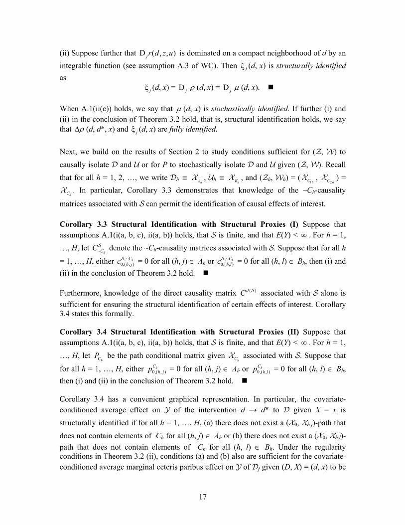
17

(ii) Suppose further that D ( , , )jr d z u is dominated on a compact neighborhood of d by an integrable function (see assumption A.3 of WC). Then ξ j (d, x) is structurally identified as

ξ j (d, x) = D j ρ (d, x) = D j µ (d, x). When A.1(ii(c)) holds, we say that µ (d, x) is stochastically identified. If further (i) and (ii) in the conclusion of Theorem 3.2 hold, that is, structural identification holds, we say that ρ∆ (d, d*, x) and ξ j (d, x) are fully identified. Next, we build on the results of Section 2 to study conditions sufficient for (Z, W) to causally isolate D and U or for P to stochastically isolate D and U given (Z, W). Recall that for all h = 1, 2, …, we write Dh ≡

hAX , Uh ≡ hBX , and (Zh, Wh) = (

1hCX , 2 hCX ) =

hCX . In particular, Corollary 3.3 demonstrates that knowledge of the ~Ch-causality

matrices associated with S can permit the identification of causal effects of interest. Corollary 3.3 Structural Identification with Structural Proxies (I) Suppose that assumptions A.1(i(a, b, c), ii(a, b)) holds, that S is finite, and that E(Y) < ∞ . For h = 1, …, H, let ~ hCCS denote the ~Ch-causality matrices associated with S. Suppose that for all h

= 1, …, H, either ,~0,( , )

hCh jcS = 0 for all (h, j) ∈ Ah or ,~

0,( , )hC

h lcS = 0 for all (h, l) ∈ Bh, then (i) and (ii) in the conclusion of Theorem 3.2 hold. Furthermore, knowledge of the direct causality matrix ( )dC S associated with S alone is sufficient for ensuring the structural identification of certain effects of interest. Corollary 3.4 states this formally. Corollary 3.4 Structural Identification with Structural Proxies (II) Suppose that assumptions A.1(i(a, b, c), ii(a, b)) holds, that S is finite, and that E(Y) < ∞ . For h = 1, …, H, let

hCP be the path conditional matrix given hCX associated with S. Suppose that

for all h = 1, …, H, either 0,( , )hCh jp = 0 for all (h, j) ∈ Ah or 0,( , )

hCh lp = 0 for all (h, l) ∈ Bh,

then (i) and (ii) in the conclusion of Theorem 3.2 hold. Corollary 3.4 has a convenient graphical representation. In particular, the covariate- conditioned average effect on Y of the intervention d → d* to D given X = x is structurally identified if for all h = 1, …, H, (a) there does not exist a (X0, Xh,j)-path that does not contain elements of Ch for all (h, j) ∈ Ah or (b) there does not exist a (X0, Xh,l)-path that does not contain elements of Ch for all (h, l) ∈ Bh. Under the regularity conditions in Theorem 3.2 (ii), conditions (a) and (b) also are sufficient for the covariate- conditioned average marginal ceteris paribus effect on Y of Dj given (D, X) = (d, x) to be

18

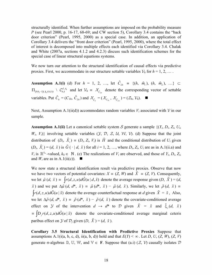
structurally identified. When further assumptions are imposed on the probability measure P (see Pearl 2000, p. 16-17, 68-69; and CW section 5), Corollary 3.4 contains the “back door criterion” (Pearl, 1995, 2000) as a special case. In addition, an application of Corollary 3.4 delivers the “front door criterion” (Pearl, 1995, 2000), where the total effect of interest is decomposed into multiple effects each identified via Corollary 3.4. Chalak and White (2007a, sections 4.1.2 and 4.2.3) discuss such identification schemes for the special case of linear structural equations systems. We now turn our attention to the structural identification of causal effects via predictive proxies. First, we accommodate in our structure settable variables Vh for h = 1, 2, … . Assumption A.1(i) (d) For h = 1, 2, …, let 2hC ≡ (h, 1m ), (h, 2m ), … ⊂

2[0: 1]( :( , ))hb A h k−Π \ ,,

hd Ah kC and let Vh ≡

2 hCX denote the corresponding vector of settable

variables. Put hC = (C1h, 2hC ) and hCX = (

1hCX , 2 hCX ) = (Zh, Vh).

Next, Assumption A.1(ii(d)) accommodates random variables Vi associated with V in our sample. Assumption A.1(ii) Let a canonical settable system S generate a sample (Yi, Di, Zi, Ui, Wi, Vi) involving settable variables (Y, D, Z, U, W, V). (d) Suppose that the joint distribution of (Di, iX ) ≡ (Di, Zi, Vi) is H and the conditional distribution of Ui given

(Di, iX ) = (d, x ) is G ( · | d, x ) for all i = 1, 2, …, where Di, Zi, Ui are as in A.1(ii.a) and Vi is 4k -valued, k4 ∈ N . (e) The realizations of Vi are observed, and those of Yi, Di, Zi, and Wi are as in A.1(ii(c)). We now state a structural identification result via predictive proxies. Observe that now we have two vectors of potential covariates: X ≡ (Z, W) and X ≡ (Z, V). Consequently, we let µ (d, x ) ≡ ( , , ) ( | , )r d z u dG u d x∫ denote the average response given (D, X ) = (d, x ) and we put µ∆ (d, d*, x ) ≡ µ (d*, x ) − µ (d, x ). Similarly, we let ρ (d, x ) ≡

( , , ) ( | )r d z u dG u x∫ denote the average counterfactual response at d given X = x , Also, we let ρ∆ (d, d*, x ) ≡ ρ (d*, x ) − ρ (d, x ) denote the covariate-conditioned average effect on Y of the intervention d → d* to D given X = x and ξ j (d, x )

≡ D ( , , ) ( | )jr d z u dG u x∫ denote the covariate-conditioned average marginal ceteris

paribus effect on Y of Dj given (D, X ) = (d, x ). Corollary 3.5 Structural Identification with Predictive Proxies Suppose that assumptions A.1(i(a, b, c, d), ii(a, b, d)) hold and that E(Y) < ∞ . Let D, U, (Z, W), (Z, V) generate σ-algebras D, U, W, and V ∈ F. Suppose that (a.i) (Z, V) causally isolates D

19

and U or (a.ii) that P stochastically isolates D and U given (Z, V); and (b.i) σ(D | V) ⊂

W ⊂ (U∨ V) or (b.ii) σ(U | V) ⊂ W ⊂ (D∨ V). Then

(i) For all (d, x) ∈ Supp (D, X), ρ∆ (d, d*, x ) is structurally identified as

ρ∆ (d, d*, x ) = µ∆ (d, d*, x ) (ii) Suppose further that D ( , , )jr d z u is dominated on a compact neighborhood of d by an

integrable function, ξ j (d, x ) is structurally identified as

ξ j (d, x ) = D j ρ (d, x ) = D j µ (d, x ) (iii) Conclusions (i) and (ii) in Theorem 3.2 hold. Consider the case where A.1(ii(e)) fails because the realizations of Vi are not observed but where A.1(i.c) holds so that the realizations of Wi are observed. In particular, suppose that (Z, V) causally isolates D and U but that (Z, W) does not causally isolate D and U.

Then it suffices that σ(D | V) ⊂ W ⊂ (U∨ V) or σ(U | V) ⊂ W ⊂ (D∨ V) to ensure

that P stochastically isolates D and U given (Z, W) and thus that ρ∆ (d, d*, x) and ξ j (d,

x) are structurally identified. Heuristically, it suffices that the information in W relates to

the information in D, U, and V in the sense discussed in Section 2.2. Observe that it is a

predictive relationship between Yi, Di, Zi, and Wi that ensures conditional exogeneity here. In particular, since (Z, W) does not causally isolate D and U, we have that the conditions for Pearl’s back door criterion do not hold here. One thus cannot conclude that structural identification holds on this basis. Nevertheless, Corollary 3.5 ensures that the covariate-conditioned average effect and marginal average effect on Y of the intervention d → d* to D given X = x are indeed structurally identified. Alternatively, suppose that A.1(ii(e)) also holds so that the realizations of both Wi and Vi are observed. Corollary 3.5 gives that ρ∆ (d, d*, x ) and ξ j (d, x ) are structurally identified and so are ρ∆ (d, d*, x) and ξ j (d, x). This “over-identification” provides a basis for constructing tests for conditional exogeneity. It is also of direct interest to construct the optimal set of covariates that ensures conditional exogeneity and delivers an efficient estimator of the conditional average and marginal effects. We leave these questions to other work. Finally, we note that although Theorem 3.2 and Corollary 3.5 are concerned with average effects, our results generalize to accommodate effects on other features of the distribution of the response, such as its variance, quantiles, or its probability distribution (see WC, section 4).

20

4. Conclusion We build on results of WC and CW to study the specification of proxies that can act as conditioning instruments to support the structural identification of causal effects of interest. In particular, we provide causal and predictive conditions sufficient for conditional exogeneity to hold, thus permitting structural identification of effects of interest. We build on results in CW to provide two procedures for inferring conditional causal isolation among vectors of settable variables in canonical settable systems. Our first procedure employs the ~A-causality matrix associated with S to state necessary and sufficient conditions for conditional causal isolation. Our second procedure employs the direct causality matrix ( )dC S associated with S to infer conditional independence relationships. The second procedure contains as a special case the notion of d-separation introduced in the artificial intelligence literature (see Pearl, 1995, 2000). It follows from CW Theorem 4.6 that these two procedures permit verifying conditional independence relationships among certain vectors of random variables in canonical settable systems. We also build on results of van Putten and Van Schuppen (1985) to provide necessary and sufficient conditions that preserve conditional independence relationships when enlarging or reducing the σ-algebras generated by the conditioning vector of variables. A corollary of this result delivers a predictive relationship among variables of interest sufficient to ensure that P is conditionally stochastically isolating. We build on these results to distinguish between two categories of conditioning instruments. The first renders the causes of interest and the unobserved direct causes of the response of interest conditionally causally isolated. Hence we refer to these as causally isolating conditioning instruments or structural proxies. We provide two procedures that permit verifying structural identification from the ~A-causality matrix associated with the structural proxies, as well as from the direct causality matrix ( )dC S . The ( )dC S -based procedure contains as a special case the “back door criterion” introduced in the artificial intelligence literature (see Pearl 1995, 2000). The second category of conditioning instruments ensures that P stochastically isolates the causes of interest and the unobserved direct causes, given the vector of conditioning instruments. We refer to this second category of conditioning instruments as stochastically isolating conditioning instruments or predictive proxies. We are unaware of any treatment of this category in the literature other than in WC and Chalak and White (2007a). Here we focus on measuring total causal effects in canonical systems. We leave to other work analysis of the measurement of direct, indirect, and the more refined notions of causality via and exclusive of sets of variables. We provide formal causal and predictive conditions sufficient to ensure that conditional exogeneity holds. We leave to other work the study of testing for conditional exogeneity, a key condition for structural identification. We also leave aside discussion of how to construct an optimal set of

21

conditioning instruments that support efficient estimation of causal effects of interest. The procedures of Section 2 should prove helpful in suggesting and testing for causal models. We also leave a formal treatment of this topic to other work. 5. Mathematical Appendix

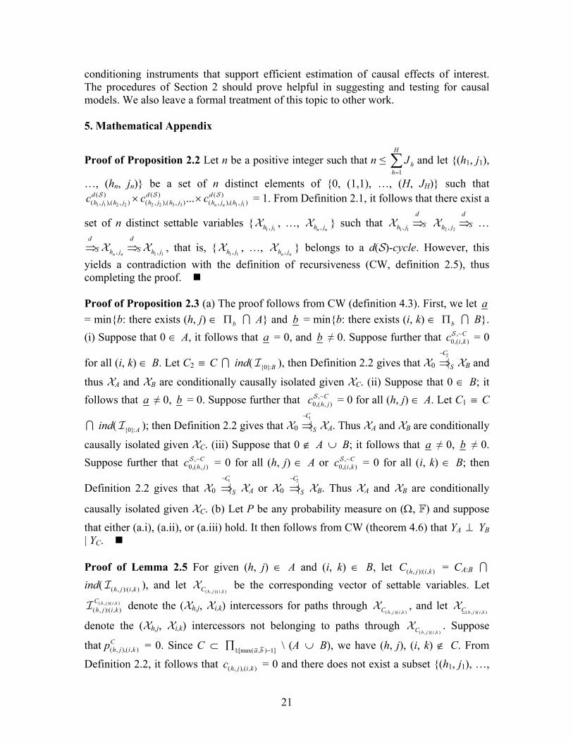
Proof of Proposition 2.2 Let n be a positive integer such that n ≤ 1

H

hh

J=

∑ and let (h1, j1),

…, (hn, jn) be a set of n distinct elements of 0, (1,1), …, (H, JH) such that

1 1 2 2 2 2 3 3 1 1

( ) ( ) ( )( , ),( , ) ( , ),( , ) ( , ),( , )...

n n

d d dh j h j h j h j h j h jc c c× ×S S S = 1. From Definition 2.1, it follows that there exist a

set of n distinct settable variables 1 1,h jX , …, ,n nh jX such that

1 1,h jX

d

S⇒ 2 2,h jX

d

S⇒ …

d

S⇒ ,n nh jX

d

S⇒1 1,h jX , that is,

1 1,h jX , …, ,n nh jX belongs to a d(S)-cycle. However, this yields a contradiction with the definition of recursiveness (CW, definition 2.5), thus completing the proof. Proof of Proposition 2.3 (a) The proof follows from CW (definition 4.3). First, we let a = minb: there exists (h, j) ∈ bΠ ∩ A and b = minb: there exists (i, k) ∈ bΠ ∩ B. (i) Suppose that 0 ∈ A, it follows that a = 0, and b ≠ 0. Suppose further that ,~

0,( , )C

i kcS = 0

for all (i, k) ∈ B. Let C2 ≡ C ∩ ind( 0:BI ), then Definition 2.2 gives that X0 2~

|C

S⇒ XB and

thus XA and XB are conditionally causally isolated given XC. (ii) Suppose that 0 ∈ B; it follows that a ≠ 0, b = 0. Suppose further that ,~

0,( , )C

h jcS = 0 for all (h, j) ∈ A. Let C1 ≡ C

∩ ind( 0:AI ); then Definition 2.2 gives that X0 1~

|C

S⇒ XA. Thus XA and XB are conditionally

causally isolated given XC. (iii) Suppose that 0 ∉ A ∪ B; it follows that a ≠ 0, b ≠ 0. Suppose further that ,~

0,( , )C

h jcS = 0 for all (h, j) ∈ A or ,~0,( , )

Ci kcS = 0 for all (i, k) ∈ B; then

Definition 2.2 gives that X0 1~

|C

S⇒ XA or X0 2~

|C

S⇒ XB. Thus XA and XB are conditionally

causally isolated given XC. (b) Let P be any probability measure on (Ω, F) and suppose

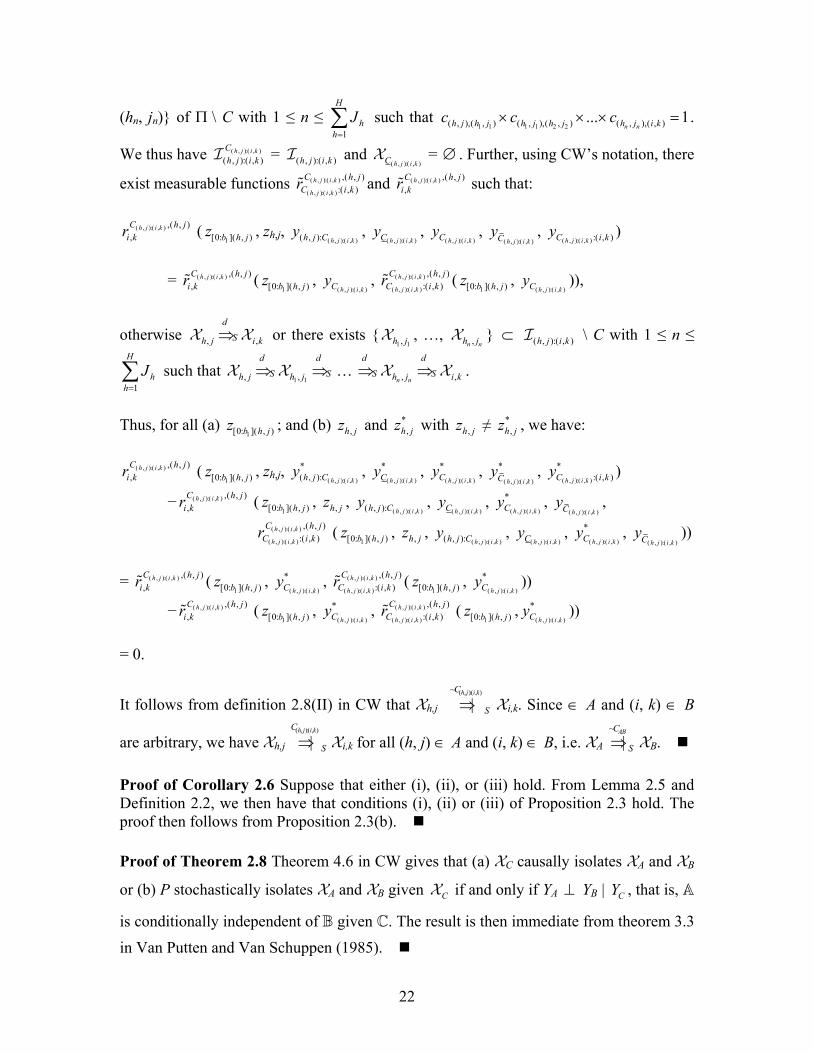
that either (a.i), (a.ii), or (a.iii) hold. It then follows from CW (theorem 4.6) that YA ⊥ YB | YC. Proof of Lemma 2.5 For given (h, j) ∈ A and (i, k) ∈ B, let ( , ):( , )h j i kC = CA:B ∩ ind( ( , ):( , )h j i kI ), and let

( , ):( , )h j i kCX be the corresponding vector of settable variables. Let ( , ):( , )

( , ):( , )h j i kC

h j i kI denote the (Xh,j, Xi,k) intercessors for paths through ( , ):( , )h j i kCX , and let

( , ):( , )h j i kCX

denote the (Xh,j, Xi,k) intercessors not belonging to paths through ( , ):( , )h j i kCX . Suppose

that ( , ),( , )Ch j i kp = 0. Since C ⊂ 1:[max( , ) 1]a b −∏ \ (A ∪ B), we have (h, j), (i, k) ∉ C. From

Definition 2.2, it follows that ( , ),( , )h j i kc = 0 and there does not exist a subset (h1, j1), …,

22

(hn, jn) of Π \ C with 1 ≤ n ≤ 1

H

hh

J=

∑ such that 1 1 1 1 2 2( , ),( , ) ( , ),( , ) ( , ),( , )... 1

n nh j h j h j h j h j i kc c c× × × = .

We thus have ( , ):( , )( , ):( , )

h j i kCh j i kI = ( , ):( , )h j i kI and

( , ):( , )h j i kCX = ∅ . Further, using CW’s notation, there

exist measurable functions ( , ):( , )

( , ):( , )

,( , ):( , )

h j i k

h j i k

C h jC i kr and ( , ):( , ) ,( , )

,h j i kC h j

i kr such that:

( , ):( , ) ,( , ),

h j i kC h ji kr (

1[0: ]( , )b h jz , zh,j, ( , ):( , )( , ): h j i kh j Cy ,

( , ):( , )h j i kCy , ( , ):( , )h j i kCy ,

( , ):( , )h j i kCy , ( , ):( , ) :( , )h j i kC i ky )

= ( , ):( , ) ,( , )

,h j i kC h j

i kr (1[0: ]( , )b h jz ,

( , ):( , )h j i kCy , ( , ):( , )

( , ):( , )

,( , ):( , )

h j i k

h j i k

C h jC i kr (

1[0: ]( , )b h jz , ( , ):( , )h j i kCy )),

otherwise ,h jX

d

S⇒ ,i kX or there exists 1 1,h jX , …, ,n nh jX ⊂ ( , ):( , )h j i kI \ C with 1 ≤ n ≤

1

H

hh

J=

∑ such that ,h jX

d

S⇒1 1,h jX

d

S⇒ … d

S⇒ ,n nh jXd

S⇒ ,i kX .

Thus, for all (a)

1[0: ]( , )b h jz ; and (b) ,h jz and *,h jz with ,h jz ≠ *

,h jz , we have:

( , ):( , ) ,( , ),

h j i kC h ji kr (

1[0: ]( , )b h jz , zh,j, ( , ):( , )

*( , ): h j i kh j Cy ,

( , ):( , )

*h j i kCy ,

( , ):( , )

*h j i kCy ,

( , ):( , )

*h j i kCy ,

( , ):( , )

*:( , )h j i kC i ky )

− ( , ):( , ) ,( , ),

h j i kC h ji kr (

1[0: ]( , )b h jz , ,h jz , ( , ):( , )( , ): h j i kh j Cy ,

( , ):( , )h j i kCy , ( , ):( , )

*h j i kCy ,

( , ):( , )h j i kCy ,

( , ):( , )

( , ):( , )

,( , ):( , )

h j i k

h j i k

C h jC i kr (

1[0: ]( , )b h jz , ,h jz , ( , ):( , )( , ): h j i kh j Cy ,

( , ):( , )h j i kCy , ( , ):( , )

*h j i kCy ,

( , ):( , )h j i kCy ))

= ( , ):( , ) ,( , )

,h j i kC h j

i kr (1[0: ]( , )b h jz ,

( , ):( , )

*h j i kCy , ( , ):( , )

( , ):( , )

,( , ):( , )

h j i k

h j i k

C h jC i kr (

1[0: ]( , )b h jz , ( , ):( , )

*h j i kCy ))

− ( , ):( , ) ,( , ),

h j i kC h ji kr (

1[0: ]( , )b h jz , ( , ):( , )

*h j i kCy , ( , ):( , )

( , ):( , )

,( , ):( , )

h j i k

h j i k

C h jC i kr (

1[0: ]( , )b h jz ,( , ):( , )

*h j i kCy ))

= 0.

It follows from definition 2.8(II) in CW that Xh,j ( , ):( , )~

|h j i kC

S⇒ Xi,k. Since ∈ A and (i, k) ∈ B

are arbitrary, we have Xh,j ( , ):( , )

|h j i kC

S⇒ Xi,k for all (h, j) ∈ A and (i, k) ∈ B, i.e. XA :~

|ABC

S⇒ XB. Proof of Corollary 2.6 Suppose that either (i), (ii), or (iii) hold. From Lemma 2.5 and Definition 2.2, we then have that conditions (i), (ii) or (iii) of Proposition 2.3 hold. The proof then follows from Proposition 2.3(b). Proof of Theorem 2.8 Theorem 4.6 in CW gives that (a) XC causally isolates XA and XB

or (b) P stochastically isolates XA and XB given CX if and only if YA ⊥ YB | CY , that is, A

is conditionally independent of B given C. The result is then immediate from theorem 3.3

in Van Putten and Van Schuppen (1985).

23

Proof of Corollary 2.9 Theorem 4.6 in CW gives that (a) XC causally isolates XA and XB

or (b) P stochastically isolates XA and XB given CX if and only if YA ⊥ YB | CY , that is, A

is conditionally independent of B given C. The result is then immediate from proposition

3.4(e) in Van Putten and Van Schuppen (1985). Proof of Lemma 3.1 Let B = ind( :( , )A i kI ), we permute the arguments of ,i krΠ to write

,,B A

i kr (2[0: 1]( :( , ))b A i kz − , Az , Bz ) ≡ ,i krΠ (

2[0: 1]bz − ). Substituting for Bz = By = ,B ABr (

2[0: 1]( :( , ))b A i kz − ,

Az ), we have ,,B A

i kr (2[0: 1]( :( , ))b A i kz − , Az , Bz ) = ,

,B A

i kr (2[0: 1]( :( , ))b A i kz − , Az , ,B A

Br (2[0: 1]( :( , ))b A i kz − , Az ))

= ,A

i kr (2[0: 1]( :( , ))b A i kz − , Az ). Fix (g, l) ∈

2[0: 1]( :( , ))b A i k−Π such that Xg,l |d

S⇒ Xi,k. Let

2[0: 1]( :( , ))( , )b A i k g lz − denote values for settings corresponding to all elements of

2[0: 1]( :( , ))( , )b A i k g l−Π = 2[0: 1]( :( , ))b A i k−Π \ (g, l). Then the function ,

Ai kr (

2[0: 1]( :( , ))b A i kz − , Az ) is constant in zg,l for every (

2[0: 1]( :( , ))( , )b A i k g lz − , zA). Thus there exists a measurable function ,( , )

,A g l

i kr such that ,( , ),A g l

i kr (2[0: 1]( :( , ))( , )b A i k g lz − , Az ) = ,

Ai kr (

2[0: 1]( :( , ))b A i kz − , Az ) for all 2[0: ]( :( , ))( , )b A i k g lz ,

zg,l, and Az . Since (g, l) ∈ 2[0: 1]( :( , ))b A i k−Π is arbitrary, it follows that there exists a

measurable function ,A

i kr such that ,A

i kr ( ,,d Ai k

zC

, Az ) = ,A

i kr (2[0: 1]( :( , ))b A i kz − , Az ) for all

,2 ,[0: 1]( :( , ))( )d A

i kb A i kz

− C, ,

,d Ai k

zC

, and Az using the obvious notation for ,2 ,[0: 1]( :( , ))( )d A

i kb A i kz

− C.

Proof of Theorem 3.2 The proof follows from theorem 3.3 in WC. (i) Suppose that A.1(i(a, b, c), ii(a, b)) hold; then assumptions A.1(a, b, c.i) in WC hold. In particular, under assumptions A.1(i(b, c)), we have that D |S⇒ Z and D |S⇒ W. Also, from Theorem

4.6 in CW we have that (a) (Z, W) causally isolates D and U or (b) P stochastically isolates D and U given (Z, W), if and only if U ⊥ D | X .Hence assumption A.2 in WC holds. Since E(Y) < ∞ , the result follows from WC (theorem 3.3 (i)). (ii) Suppose further that D ( , , )jr d z u is dominated on a compact neighborhood of d by an integrable function, then assumption A.3 in WC holds and the result follows from WC (theorem 3.3 (ii)). Proof of Corollary 3.3 Since 0 ∉ Ah ∪ Bh for all h = 1, …, H, Proposition 2.3 gives that Dh and Uh are conditionally causally isolated given (Zh, Wh) and thus D ⊥ U | X. The result then follows from Theorem 3.2. Proof of Corollary 3.4 Since 0 ∉ Ah ∪ Bh, for all h = 1, …, H, Corollary 2.6 gives that Dh and Uh are conditionally causally isolated given (Zh, Wh) and thus D ⊥ U | X. The result then follows from Theorem 3.2.

24

Proof of Corollary 3.5 Suppose that (a.i) or (a.ii); and (b.i) or (b.ii) hold. Then, from Corollary 2.9, we have that (Z, W) causally isolates D and U or that P stochastically isolates D and U given (Z, W). The result then follows from Theorem 3.2. References

Bang-Jensen, J. and G. Gutin (2001). Digraphs: Theory, Algorithms and

Applications. London: Springer-Verlag.

Blundell, R. and J. Powell (2003), “Endogeneity in Nonparametric and

Semiparametric Regression Models,” in M. Dewatripoint, L. Hansen, and S. Turnovsky

(eds.), Advances in Economics and Econometrics: Theory and Applications, Eighth

World Congress, Vol II. New York: Cambridge University Press, 312-357.

Chalak, K., and H. White (2007a), “An Extended Class of Instrumental Variables for

the Estimation of Causal Effects,” UCSD Department of Economics Discussion Paper.

Chalak, K. and H. White (2007b), “Independence and Conditional Independence in

Causal Systems,” UCSD Department of Economics Discussion Paper.

Heckman, J. and R. Robb (1985), “Alternative Methods for Evaluating the Impact of

Interventions,” in J. Heckman and B. Singer (eds.), Longitudinal Analysis of Labor

Market Data. Cambridge: Cambridge University Press, 146-245.

Heckman, J. and B. Honore (1990), “The Empirical Content of the Roy Model,”

Econometrica, 58, 1121-1149.

Heckman, J. and E. Vytlacil (2005), “Structural Equations, Treatment Effects, and

Econometric Policy Evaluation,” Econometrica, 73, 669-738.

Matzkin, R. (2003), “Nonparametric Estimation of Nonadditive Random Functions,”

Econometrica, 71, 1339-1375.

Pearl, J. (1995), “Causal Diagrams for Empirical Research,” Biometrika, 82, 669-710

(with Discussion).

Pearl, J. (2000). Causality: Models, Reasoning, and Inference. New York: Cambridge

University Press.

Rosenbaum, P. R. (2002). Observational Studies. 2nd ed., Berlin: Springer-Verlag.

Rosenbaum, P. R. and D. Rubin (1983), “The Central Role of the Propensity Score in

Observational Studies for Causal Effects,” Biometrika, 70, 41-55.

25

Rubin, D. (1974), “Estimating Causal Effects of Treatments in Randomized and Non-

randomized Studies,” Journal of Educational Psychology, 66, 688-701.

Van Putten, C. and J.H. Van Schuppen, (1985), “Invariance Properties of the

Conditional Independence Relation,” The Annals of Probability, 13, 934-945.

White, H. and K. Chalak (2006), “A Unified Framework for Defining and Identifying

Causal Effects,” UCSD Department of Economics Discussion Paper.