karl pearson's meta-analysis revisited - stanford...

Karl Pearson’s meta-analysis revisited

Art B. Owen∗

Department of StatisticsSequoia Hall

390 Serra MallStanford CA 94305

e-mail: [email protected]: http://stat.stanford.edu/∼owen

Abstract: This paper revisits a meta-analysis method proposed byPearson (1934) and first used by David (1933). It was thought to beinadmissible, for over fifty years, dating back to a paper of Birnbaum(1954). It turns out that the method Birnbaum analyzed is not the onethat Pearson proposed. We show that Pearson’s proposal is admissible.Because it is admissible it has better power than the standard test ofFisher (1932) at some alternatives, worse power at others. Pearson’smethod has the advantage when all or most of the nonzero parametersshare the same sign. Pearson’s test has proved useful in a genomic set-ting, screening for age-related genes. This paper also presents an FFTbased method for getting hard upper and lower bounds on the CDF ofa sum of nonnegative random variables.

1. Introduction

Methods for combining p-values have long been studied. Recent researchin genomics (Zahn et al., 2007) and functional magnetic resonance imaging(fMRI) (see references in Benjamini and Heller (2007)) has sparked renewedinterest. One gets a large matrix of p-values and considers meta-analysisalong the rows, controlling for multiplicity issues in the resulting column ofcombined p-values.

This paper revisits an old issue in meta-analysis. A genomic applicationlead to the re-invention of a meta-analysis technique of K. Pearson (1934).That method has long been out of favor, because the paper of Birnbaum(1954) appears to have proved that it is inadmissible (in an exponentialfamily context). This paper shows that the method is in fact admissible inthat exponential family context. Being admissible, it is more powerful thanthe widely used combination method of Fisher (1932) at some points of the

∗This work was supported by grant DMS-0604939 from the U.S. National ScienceFoundation.

1

imsart-generic ver. 2007/12/10 file: articleR1.tex date: January 9, 2009

mailto:[email protected]

http://stat.stanford.edu/$sim $owen

/Pearson’s meta-analysis 2

alternative hypothesis. Such points turn out to be especially important inthe motivating biological problem.

The motivating work, reported in the AGEMAP study of Zahn et al.(2007), was to screen 8932 genes, searching for those having expression levelsthat are correlated with age in the mouse. Each gene was tested in m = 16tissues, yielding 16 regression coefficients. There was an 8932×16 matrix of pvalues. The data were noisy and it was plausible a priori that most if not allgenes could have little or no correlation with age. In addition to the recentlywell studied issue of controlling for multiple testing over genes, there was aproblem of pooling information from different tissues for any single gene. Forissues of multiple testing see Dudoit and van der Laan (2008). This articlefocuses on the problem of basing a single test on m > 1 test statistics.

A gene that is not age-related has a slope parameter of zero in all mtissues. For a gene that is age-related we expect several nonzero slopes.Because gene expression is tissue dependent it is also possible that a genecorrelated with age in numerous tissues might fail to correlate in some others.Therefore, assuming a common non-zero slope is unreasonable. It is evenpossible that a gene’s expression could increase with age in some tissueswhile decreasing in one or more others. But we do expect that the non-zeroslopes should be predominantly of the same sign. The prior understandingof the biology is not detailed enough to let us specify in advance how manytissues might be non age-related or even discordant, for an otherwise age-related tissue.

Pearson’s method is well suited to this problem. The better known methodof Fisher combines p-values by taking their product. It can be based onone-tailed or two-tailed test statistics. When based on one-tailed statistics,Fisher’s test works best if we know the signs of the alternatives. When basedon two-tailed statistics, Fisher’s test does not favor alternatives that sharea common sign. The test of Pearson (1934) may be simply described. Itruns a Fisher style test for common left sided alternatives as well as one forcommon right sided alternatives and it takes whichever of those two is mostextreme. It builds in a strong preference for common directionality while notrequiring us to know the common direction, and it remains powerful whena small number of tests have sign different from the dominant one. Theseproperties fit the needs in Zahn et al. (2007).

An outline of this paper is as follows. Section 2 defines the test statisticsand hypotheses that we work with. Section 3 reviews some basic concepts inmeta analysis and compares Pearson’s test graphically to the better knowncompetitors. Section 4 shows that Pearson’s method is admissible in theexponential family context. It also shows that a simple factor of two Bonfer-



roni correction is very accurate for tail probabilities based on Pearson’s teststatistic. Section 5 reviews the history surrounding the misinterpretation ofPearson’s proposal. Part of the problem stems from mixing up p-values fromone and two-tailed tests. Section 6 compares the power of Pearson’s test withsome others, including tests that are based on the original test statistics notjust the p-values. Section 7 considers some of the recent literature on com-bining p-values. A discussion is in Section 8. The appendix presents thenumerical methods used to make the power computations. These are basedon a kind of interval arithmetic for subdistributions using the FFT.

2. Notation

This section sets out the notation for the paper. First are the parameters,hypotheses and test statistics for the univariate settings. Then they arecombined to define multivariate rejection regions and test statistics.

2.1. Parameters and hypotheses

We consider a setting where there are m parameters β1, . . . , βm and m corre-sponding estimates β1, . . . , βm. These estimates are random variables whoseobserved values are denoted by βobs

1 , . . . , βobsm . In the motivating problem

these were regression slopes. We assume that the m statistics βj are inde-pendent. Dependent test statistics are considered briefly in Section 6.3. Wealso assume that βj have continuous distributions.

For j = 1, . . . ,m, we can consider the hypotheses

H0,j : βj = 0HL,j : βj < 0HR,j : βj > 0, and,HU,j : βj 6= 0,

based on the sign of βj . These are the null hypotheses, left and right-sidedalternatives and an undirected alternative, respectively.

Using βobsj as test statistics, we may define

pj = Pr(βj ≤ βobsj | βj = 0), and,

pj = Pr(|βj | ≥ |βobsj | | βj = 0).

The p-values for alternatives HL,j , HR,j and HU,j , respectively, are pj , 1−pj ,and pj = 2min(pj , 1 − pj). A p-value for a one-tailed or two-tailed test iscalled a one-tailed or two-tailed p-value below.



For the entire parameter vector β = (β1, . . . , βm) it is straightforward todefine the simple null hypotheses H0 for which β1 = β2 = · · · = βm = 0. Wedo not consider composite null hypotheses.

For m > 1 the alternatives to H0 are more complicated than for m = 1.There are 3m possible values for the vector of signs of βj values and manypossible subsets of these could be used to define the alternative. For exampleone could take

HL = (−∞, 0]m − {0} or HR = [0,∞)m − {0}

or their union.But any of these choices leaves out possibilities of interest. Therefore we

take the alternative HA to be that βj 6= 0 for at least one j ∈ {1, . . . ,m}.That is HA : β ∈ Rm − {0}.

While all of Rm−{0} is of interest, the parts with concordant signs are ofgreater interest than those with discordant signs. For example with ∆ > 0 wewant greater power against alternatives ±(∆,∆, . . . ,∆) than against otheralternatives of the form (±∆,±∆, . . . ,±∆). In a screening problem, theformer are more convincing while the latter cause one to worry about noiseand systematic experimental biases. The situation is analogous to the choiceof the Tukey’s versus Sheffe’s statistic in multiple comparisons: both havethe alternative of unequal means, but their power versus specific alternativesof interest could lead us to prefer one to the other in a given application.

It is worthwhile to represent the vector β as the product τθ where θ ∈ Rm

is a unit vector and τ ≥ 0. We may then consider the power of various testsof H0 as τ increases.

2.2. Rejection regions

The decision to accept or reject H0 will be based on p1, . . . , pm. As usual,acceptance really means failure to reject and is not interpreted as establish-ing H0. The rejection region is R = {(p1, . . . , pm) | H0 rejected} ⊂ [0, 1]m.For some of the methods we consider, the rejection region can be expressedin terms of the two-tailed p-values pj . Then we write R = {(p1, . . . , pm) |H0 rejected} ⊂ [0, 1]m.

While formulating the region in terms of p values seems unnatural whenthe raw data are available, it does not change the problem much. For ex-ample if βj ∼ N (βj , σ

2j ) with known σ2

j then any region defined throughpj values can be translated into one for βj values. In that case we writeR′ = {(β1, . . . , βm) | H0 rejected}. It is more realistic for the p-values to



come from a t distribution based on estimates of σ2j . For large degrees of

freedom the normal approximation to the t distributed problem is a reason-able one and it is simpler to study. Discussion of t distributed test statisticsis taken up briefly in Section 6.1.

2.3. Test statistics

Under the null hypothesis pj , 1− pj , and pj all have the U(0, 1) distribution.It follows that

QL ≡ −2 log( m∏

j=1

pj

), (2.1)

QR ≡ −2 log( m∏

j=1

(1− pj))

, and, (2.2)

QU ≡ −2 log( m∏

j=1

pj

)(2.3)

all have the χ2(2m) distribution under H0. An α level test based on any of

these quantities rejects H0 when that Q is greater than or equal to χ2,1−α(2m) .

Their chisquare distribution is due to Fisher (1932).When m = 1 these three tests reduce to the usual one and two sided tests.

When m > 1 they are reasonable generalizations of one and two sided tests.The test of K. Pearson (1934) is based on

QC ≡ max(QL, QR). (2.4)

If m = 1 then QC = QU , but for m > 1 they differ. The superscript C ismnemonic for concordant.

The null distribution of QC is not χ2(2m). However a Bonferroni correction

is quite accurate:

α− α2

4≤ Pr(QC ≥ χ

2,1−α/2(2m) ) ≤ α. (2.5)

Equation (2.5) follows from Corollary 1 in Section 4. For instance when thenominal level is α = 0.01, the attained level is between 0.01 and 0.009975.Equation (2.5) shows that min(1, 2 Pr(χ2

(2m) ≥ QC)) is a conservative pvalue. Equation 2.5 shows that the accuracy of this Bonferroni inequalityimproves for small α which is where we need it most.



The statistic QL is the natural one to use when the alternative is knownto be in HL. But it still has power tending to 1 as τ = ‖β‖ tends to infinityso long as θ = β/τ is not in HR. Naturally QR has a similar problem in HL

while being well suited for HR. Neither QC nor QU have such problems. Ifwe have no idea which orthant β might be in then QU is a natural choice,while if we suspect that the signs of large (in absolute value) nonzero βj aremostly the same, then QC has an advantage over QU .

2.4. Stouffer et al.’s meta-analysis

An alternative to Fisher’s method is that of Stouffer et al. (1949), which isbased on turning the p values into Z-scores. Let ϕ(x) = exp(−x2/2)/

√2π

denote the N (0, 1) density and then let Φ(x) =∫ x−∞ ϕ(z) dz.

We can define tests of H0 based on Z-scores via

SL =1√m

m∑j=1

Φ−1(1− pj) (2.6)

SR =1√m

m∑j=1

Φ−1(pj) (2.7)

SU =1√m

m∑j=1

|Φ−1(pj)|, and, (2.8)

SC = max(SL, SR), (2.9)

directly analogous to the tests of Section 2.3. For independent tests consid-ered here, SL and SR have the N (0, 1) distribution under H0, while SC hasa half-normal distribution and SU does not have a simple distribution. Notethat SL = −SR and that SC = |SL| = |SR|.

3. Meta-analysis and a graphical comparison of the tests

This section reviews some basics of meta-analysis for further use. Then itpresents a graphical comparison of Pearson’s test with the usual tests, toshow how it favors alternatives with concordant signs. For background onmeta-analysis see Hedges and Olkin (1985).

It has been known since Birnbaum (1954) that there is no single bestcombination of m independent p-values. A very natural requirement for acombination test is Birnbaum’s



Condition 1. If H0 is rejected for any given (p1, . . . , pm), then it will alsobe rejected for all (p∗1, . . . , p

∗m) such that p∗j ≤ pj for j = 1, . . . ,m.

Birnbaum proved that every combination procedure which satisfies Con-dition 1 is in fact optimal, for some monotone alternative distribution. Op-timality means maximizing the probability of rejecting H0 subject to a con-straint on the volume of the region R of vectors (p1, . . . , pm) for which H0 isrejected. Birnbaum allows simple alternatives that have independent pj withdecreasing densities gj(pj) on 0 ≤ pj ≤ 1. He also allows Bayes mixtures ofsuch simple alternatives. Birnbaum shows that Condition 1 is necessary andsufficient for admissibility of the combination test, again in the context ofdecreasing densities. Here is his definition of admissibility:

Definition 1 (Birnbaum, 1954, page 564). A test is admissible if there isno other test with the same significance level which, without ever being lesssensitive to possible alternative hypotheses, is more sensitive to at least onealternative.

The top row of Figure 1 illustrates 4 rejection regions R satisfying Con-dition 1, arising from the Fisher test, the Stouffer test, a test based onmin(p1, . . . , pm) and a test based on max(p1, . . . , pm), for the case m =2. Using the minimum is due to Tippett (1931), while the maximum isfrom Wilkinson (1951), who is credited with the more general approach ofusing an order statistic of the pj .

The criterion min(p1, p2) leads us to reject H0 if either test 1 or test 2is strongly significant. The criterion max(p1, p2) is similarly seen to requireat least some significance from both test 1 and test 2. Birnbaum’s resultopens up the possibility for many combinations between these simple typesof which Fisher’s test and Stouffer’s test are two prominent examples.

Graphically, we see that Fisher’s combination is more sensitive to the sin-gle smallest p value than Stouffer’s combination is. In the Fisher test, if thefirst m− 1 p-values already yield a test statistic exceeding the χ2

(2m) signif-icance threshold then the m’th test statistic cannot undo it. The Stouffertest is different. Any large but finite value of

∑m−1j=1 Φ−1(pj) can be cancelled

by an opposing value of Φ−1(pm).The bottom row of Figure 1 illustrates the pre-images (p1, p2), where

pj = 2 min(pj , 1 − pj), of the regions in the top row. Those images showwhich combinations of one sided p-values lead to rejection of H0. Each regionR in the bottom row of Figure 1 is symmetric with respect to replacing pj

by 1− pj , and so they do not favor alternatives with concordant signs.Figure 2 shows the rejection regions for concordant versions of the Fisher



Fig 1. This figure shows rejection regions for a pair of tests. The top four images havecoordinates (p1, p2) where pj near zero is evidence against H0j in a two tailed test. Thecolumns, from left to right, are based on min(p1, p2), max(p1, p2), Fisher’s combinationand Stouffer’s combination, as described in the text. Each region has area 1/10. The bottomrow shows the same rejection regions in coordinates (p1, p2) where pj near 0 is evidencethat βj < 0 and pj near 1 is evidence that βj > 0.

and Stouffer tests. Both of these regions devote more area to catching coor-dinated alternatives to H0 than to split decisions. Comparing the upper leftand lower right corners of these regions we see that the Stouffer version ismore extreme than the Fisher test in rejecting split decisions.

A naive reading of Condition 1 is that almost any p value combination isreasonable. But some of those combinations are optimal for very unrealisticalternatives. Birnbaum (1954) goes deeper by considering alternatives in anexponential family, beginning with his second condition

Condition 2. If test statistic values (β1, . . . , βm) and (β∗1 , . . . , β∗m) do notlead to rejection of H0, then neither does λ(β1, . . . , βm)+(1−λ)(β∗1 , . . . , β∗m)for 0 < λ < 1.

Condition 2 requires that the acceptance region, in test statistic space,be convex. If the test statistics being combined are from a one parameterexponential family, then Birnbaum (1954) shows that Condition 2 is nec-essary for the combined test to be admissible. When the parameter spaceis all of Rm then Condition 2 is also sufficient for the combined test to beadmissible. This is a consequence of the theorem in Stein (1956, Section3). Birnbaum (1955) had this converse too, but without a condition on un-



Fig 2. This figure shows rejection regions R for concordant tests, QC and SC , as describedin the text. The left image shows a region for Pearson’s QC which is based on Fisher’scombination. The right image shows a region for SC , based on Stouffer’s combination.The x and y axes in these images correspond to one sided p values p1 and p2, rejectingH0 for negative slopes at the bottom and/or left, while rejecting H0 for positive slopes atthe top and/or right. These tests are more sensitive to alternatives where all underlyinghypothesis tests reject in the same direction than they are to split decisions. The Stoufferregion extends to all corners but with a thickness that approaches zero. The Fisher regionhas strictly positive thickness in each corner.

boundedness of the parameter space. Matthes and Truax (1967) prove thatthe unboundedness is needed. Thus Condition 2 is reasonable and it rulesout conjunction-based tests like the one based on max(p1, . . . , pm) and moregenerally, all of the Wilkinson methods based on p(r) for 1 < r ≤ m.

Suppose that βj ∼ N (βj , 1). Then Birnbaum (1954) shows that a testwhich rejects H0 when

∏mj=1(1−pj) is too large, fails Condition 2. For small

α and m = 2 that test has a nearly triangular rejection region R including(0, 0) in the (p1, p2) plane. For small α it would not reject at (p1, p2) = (0, 1)or even at (0, 0.5). Birnbaum (1955) attributes that test to Karl Pearsonthrough a description given by E. S. Pearson (1938). But Karl Pearson didnot propose this test and it certainly is not QC . It appears that Birnbaumhas misread Egon Pearson’s description of Karl Pearson’s test. A detaileddiscussion of that literature is given in Section 5.

Theorem 1 in Section 4 shows that QC satisfies Condition 2 for normallydistributed test statistics, and so it is admissible. Figure 3 illustrates someacceptance regions for QU , QC , QL, and

∏mj=1(1− pj).



Fig 3. This figure shows nested decision boundaries in the space of test statistics β =(β1, . . . , βm) for meta-analysis methods described in the text. We are interested in theregions where H0 is not rejected. From left to right they are: Fisher’s combination QU

with lozenge shaped regions, Pearson’s combination QC with leaf shaped regions, a left-sided combination QL with quarter-round shaped regions north-east of the origin, andBirnbaum’s version of Pearson’s region, having non-convex plus sign shaped regions. Ineach plot the significance levels are at 0.2, 0.1, 0.05, and 0.01.

In applications, Fisher’s method is more widely used than Stouffer’s. Ina limit where sample sizes increase and test statistics become more nearlynormally distributed, some methods are maximally efficient in Bahadur’ssense (Bahadur, 1967). Fisher’s method is one of these, and Stouffer’s isnot. See Table 3 on page 44 of Hedges and Olkin (1985). Both Birnbaum(1954) and Hedges and Olkin (1985) consider Fisher’s method to be a kindof default, first among equals or better.

4. Pearson’s combination

In this section we prove two properties of Pearson’s combination QC . Theacceptance regions in the second panel of Figure 3 certainly appear to beconvex. We prove that his test satisfies Condition 2 (convexity), for Gaussiantest statistics. Therefore it is in fact admissible in the exponential family con-text for the Gaussian case. The result extends to statistics with log-concavedensities. Finally we show that the Bonferroni bound on the combination isvery accurate for small combined p values.

4.1. Propagation of admissibility to QC

We consider first the setting of Gaussian test statistics βj ∼ N (βj , σ2/nj).

For simplicity we work in terms of tj = √nj βj/σ. Under H0 the tj are IID

N (0, 1). The proof that QC is admissible uses rules that propagate convexityand quasi-convexity. It is broken into small pieces that are used for othertest statistics in Sections 6 and 7.



Let Q(t1, . . . , tm) be a real valued function on Rm. The associated testrejects H0 in favor of HA when Q ≥ q. That test is admissible in the expo-nential family context if {(t1, . . . , tm) | Q < q} is convex and the naturalparameter space is Rm.

Lemma 1. For k = 1, . . . , n, suppose that the test which rejects H0 versusHA when Qk(t1, . . . , tm) ≥ qk is admissible in the exponential family contextwith natural parameter space Rm. Let the test based on Qk have level αk.Then the test which rejects H0 when one or more of Qk(t1, . . . , tm) ≥ qk

hold is also admissible and has level α ≤∑n

k=1 αk.

Proof. Under the assumptions, the acceptance regions for the n individualtests are convex. The combined test has an acceptance region equal to theirintersection which is also convex. Therefore the combined test is admissible.The level follows from the Bonferroni inequality.

Lemma 2. For k = 1, . . . , n, suppose that a test rejects H0 versus HA whenQk(t1, . . . , tm) ≥ qk where Qk is a convex function on Rm. Then the testwhich rejects H0 when Q(t1, . . . , tm) =

∑nk=1 Qk(t1, . . . , tm) ≥ q holds is

admissible in the exponential family context with natural parameter spaceRm.

Proof. Under the assumptions, each Qk is a convex function, and so thereforeis their sum Q. Then {(t1, . . . , tm) | Q < q} is convex and so the test isadmissible.

Given a battery of admissible tests, Lemma 1 shows that we can run themall and get a new admissible test that rejects H0 if any one of them rejects.Lemma 2 shows that for tests that have convex criterion functions, we cansum those functions and get a test criterion for another admissible test.Lemma 2 requires a stronger condition on the component tests Qk thanLemma 1 does. Aside from the difference between open and closed levelsets, the criterion used in Lemma 1 is quasi-convexity. Sums of quasi-convexfunctions are not necessarily quasi-convex (Greenberg and Pierskalla, 1971).

Theorem 1. For t1, . . . , tm ∈ Rm let

QC = max(−2 log

m∏j=1

Φ(tj),−2 logm∏

j=1

Φ(−tj))

.

Then {(t1, . . . , tm) | QC < q} is convex so that Pearson’s test is admissiblein the exponential family context, for Gaussian data.



Proof. The function Φ(t) is log concave. Therefore the test that rejects H0

when Qk = −2 log Φ(tk) is large (ignoring the other m − 1 statistics) hasa convex criterion function. Applying Lemma 2 to those tests shows thatthe test based on QL = −2

∑mj=1 log(Φ(tj)) has convex acceptance regions.

The same argument starting with log concavity of Φ(−t) shows that the testbased on QR = −2

∑mj=1 log(Φ(−tj)) has convex acceptance regions. Then

Lemma 1 applied to QL and QR shows that QC has convex acceptanceregions.

The Gaussian case is concrete and is directly related to the motivatingcontext. But the result in Theorem 1 holds more generally. Suppose that thedensity functions (d/dt)Fj(t) exists and are log concave for j = 1, . . . ,m.Then both Fj(t) and 1 − Fj(t) are log concave (Boyd and Vandeberghe,2004, Chapter 3.5). Then the argument from Theorem 1 shows that the testcriteria QL = −2

∑j log(Fj(tj)), QR = −2

∑j log(1 − Fj(tj)), and QC =

max(QL, QR) all have convex acceptance regions.While many tests built using Lemmas 1 and 2 are admissible in the ex-

ponential family context it may still be a challenge to find their level. Thenext section takes up the issue of bounding α for tests like QC .

4.2. Bonferroni

Here we show that the Bonferroni bound for QC is very accurate, in the tailswhere we need it most. The Bonferroni bound for QC is so good because itis rare for both QL and QR to exceed a high level under H0. For notationalsimplicity, this section uses Xj in place of pj .

Theorem 2. Let X = (X1, . . . , Xm) ∈ (0, 1)m be a random vector withindependent components, and put

QL ≡ −2 log( m∏

j=1

Xj

), QR ≡ −2 log

( m∏j=1

(1−Xj))

,

and QC = max(QL, QR). For A ∈ R, let PL = Pr(QL > A), PR = Pr(QR >A), and PT = Pr(QC > A). Then PL + PR − PLPR ≤ PT ≤ PL + PR.

Corollary 1. Suppose that X ∼ U(0, 1)m in Theorem 2. For A > 0 letτA = Pr(χ2

(2m) > A). Then

2τA − τ2A ≤ Pr(QC > A) ≤ 2τA.



Proof. When X ∼ U(0, 1)m, then Pr(QL > A) = Pr(QR > A) = τA. Theresult follows by substitution in Theorem 2.

Before proving Theorem 2 we present the concept of associated randomvariables, due to Esary, Proschan, and Walkup (1967).

Definition 2. A function f on Rn is nondecreasing if it is nondecreasing ineach of its n arguments when the other n− 1 values are held fixed.

Definition 3. Let X1, . . . , Xn be random variables with a joint distribution.These random variables are associated if Cov(f(X), g(X)) ≥ 0 holds for allnondecreasing functions f and g for which the covariance is defined.

Lemma 3. Independent random variables are associated.

Proof. See Section 2 of Esary, Proschan, and Walkup (1967).

Lemma 4. For integer m ≥ 1 let X = (X1, . . . , Xm) ∈ (0, 1)m have inde-pendent components. Set

QL = −2 logm∏

j=1

Xj , and, QR = −2 logm∏

j=1

(1−Xj).

Then for any AL > 0 and AR > 0,

Pr(QL > AL, QR > AR) ≤ Pr(QL > AL) Pr(QR > AR).

Proof. Let f1(X) = 2 log∏m

j=1 Xj and f2(X) = −2 log∏m

j=1(1 −Xj). Thenboth f1 and f2 are nondecreasing functions of X. The components of X areindependent, and hence are associated. Therefore

Pr(QL > AL, QR > AR) = Pr(−f1(X) > AL, f2(X) > AR)= Pr(f1(X) < −AL, f2(X) > AR)= Pr(f2(X) > AR)− Pr(f1(X) ≥ −AL, f2(X) > AR)≤ Pr(f2(X) > AR)− Pr(f1(X) ≥ −AL) Pr(f2(X) > AR)= Pr(f2(X) > AR) Pr(f1(X) < −AL)

= Pr(QR > AR) Pr(QL > AL).

In general, nondecreasing functions of associated random variables are as-sociated. Lemma 4 is a special case of this fact, for certain indicator functionsof associated variables.



Proof of Theorem 2. The Bonferroni inequality yields PT ≤ PL+PR. FinallyPT = PL + PR − Pr(QL > A,QR > A) and Pr(QL > A,QR > A) ≤ PLPR

from Lemma 4.

Remark 1. The same proof holds for combinations of many other testsbesides Fisher’s. We just need the probability of simultaneous rejection tobe smaller than it would be for independent tests.

5. History of Pearson’s test

Pearson (1933) proposed the product∏n

i=1 F0(Xi) as a way of testing whetherIID observations X1, . . . , Xn are from the distribution with CDF F0. He findsthe distribution of the product in terms of incomplete gamma functions andcomputes several examples. Pearson remarks that the test has advantagesover the χ2 test of goodness of fit: small groups of observations don’t have tobe pooled together, and one need not approximate small binomial counts bya normal distribution. Pearson also notices that the approach is applicablemore generally than testing goodness of fit for IID data, and in a note atthe end, acknowledges that Fisher (1932) found the distribution earlier.

In his second paper on the topic, Pearson (1934) found a p-value for∏j F (Xj) and one for

∏j(1−F (Xj)) and then advocated taking the smaller

of these two as the “more stringent” test. Modern statisticians would in-stinctively double the smaller p-value thereby applying a Bonferroni factorof 2, but Pearson did not do this.

Birnbaum (1954, page 562) describes a test of Karl Pearson as follows

“Karl Pearson’s method: reject H0 if and only if (1 − u1)(1 − u2) · · · (1 − uk) ≥ c,where c is a predetermined constant corresponding to the desired significance level. Inapplications, c can be computed by a direct adaptation of the method used to calculatethe c used in Fisher’s method.”

In the notation of this paper (1 − u1)(1 − u2) · · · (1 − uk) is∏m

j=1(1 − pj),for Figure 4 of Birnbaum (1954), and it is

∏mj=1(1 − pj) for Figure 9. The

latter (but not the former) would lead to an admissible test had the rejectionregion been for small values of the product.

Birnbaum does not cite any of Karl Pearson’s papers directly, but doescite Egon Pearson (1938) as a reference for Karl Pearson’s test. E. Pearson(1938, page 136) says:

“Following what may be described as the intuitional line of approach, K. Pearson(1933) suggested as suitable test criterion one or other of the products

Q1 = y1y2 · · · yn,

or Q′1 = (1− y1)(1− y2) · · · (1− yn).”



The quotation above omits two equation numbers and two footnotes butis otherwise verbatim. In the notation of this paper Q1 =

∏mj=1 pj and

Q′1 =

∏mj=1(1 − pj). E. Pearson cites K. Pearson’s 1933 paper, although

it appears that he should have cited the 1934 paper instead, because theformer has only Q1, while the latter has Q1 and Q′

1.Birnbaum (1954) appears to have read E. Pearson’s article as supplying

two different proposals of K. Pearson and then to have chosen the one basedQ′

1, rejecting for large values of that product.In an article published after Pearson (1933) but before Pearson (1934),

David (1934, page 2) revisits the 12 numerical examples computed by Pear-son (1933) and reports that in 4 of those, Pearson had made a wrong guessas to which of Q1 and Q′

1 would be smaller:

“Thus in 8 of the 12 illustrations the more stringent direction of the probabilityintegrals was selected by mere inspection. In the other 4 cases B ought to have beentaken instead of A, but in none of these four cases was the difference such as to upsetthe judgment as to randomness deduced from A.”

Pearson (1933) computed Q1 all 12 times and does not mention that thisis a guess as to which product is smaller. Thus it is David’s paper in whichmin(Q1, Q

′1) is first used (as opposed to Q1). One might therefore credit

David with this test, as for example, Oosterhoff (1969) does. But Davidcredits Pearson for the method.

Birnbaum’s conclusion about Pearson’s test is now well established in theliterature. Hedges and Olkin (1985, page 38) write

“Several other functions for combining p-values have been proposed. In 1933 KarlPearson suggested combining p-values via the product

(1− p1)(1− p2) · · · (1− pk).

Other functions of the statistics p∗i = Min{pi, 1 − pi}, i = 1, . . . , k, were suggested by

David (1934) for the combination of two-sided test statistic, which treat large and smallvalues of the pi symmetrically. Neither of these procedures has a convex acceptanceregion, so these procedures are not admissible for combining test statistics from theone-parameter exponential family.”

The pi in this quotation might refer to either pi or pi in the notation ofthis paper. If the former, then the product would be equivalent to QR andwould be admissible. If the latter, then the product would conform to thestatistic that Birnbaum studies, but not the one Karl Pearson proposed.Furthermore, in that case the quantity p∗i = min(pi, 1 − pi) vanishes atpi ∈ {0, 1/2, 1} and takes its maximal value at pi ∈ {1/4, 3/4}, which doesnot make sense.



6. Power comparisons

Admissibility of QC is historically interesting, but for practical purposes wewant to know how its power compares to other test statistics such as undi-rected ones, Stouffer based ones, and some likelihood ratio tests developedbelow.

In this section we compare the power of these tests at some alternativesof the form (∆, . . . ,∆, 0, . . . , 0) for ∆ > 0 where k components are nonzeroand m − k are zero. Alternatives of the form (−∆,∆, . . . ,∆, 0, . . . , 0) for∆ > 0 are also investigated.

Not surprisingly, concordant tests generally outperform their undirectedcounterparts. The most powerful method depends on the value of k. In ap-plications where we know roughly how many nonzero and discordant slopesto expect, we can then identify which method will be most powerful, usingthe methods in this section.

The power of tests based on SL, SR, and SC can be handled via the nor-mal CDF. The statistics QL, QR, QU , and SU are all sums of m independentnonnegative random variables. It is therefore possible to get a good approx-imation to their exact distributions via the fast Fourier transform (FFT).For each of them, we use the FFT first to find their critical level (exceededwith small probability α). The FFT is used in such a way as to get hardupper and lower bounds on the cumulative probabilities which yield hardupper and lower bounds for the critical value. Then a second FFT underthe alternative hypothesis is used to compute their power. The upper limitof the power of some Q comes from the upper bound on the probability ofQ exceeding the lower bound on its critical value. The lower limit of poweris defined similarly.

For QC , the upper and lower limits on the critical value come via (2.5)applied to the bounds for QL and QR. So does the power.

All the computations were also done by simple Monte Carlo, with 99.9%confidence intervals. Usually the 100% intervals from the FFT were narrowerthan the MC intervals. But in some cases where (2.5) is not very tight, suchas concordant tests at modest power, the MC intervals came out narrower.

6.1. Alternatives to meta-analysis

In the AGEMAP study all of the original data were present and so onecould use them to form the usual test statistics instead of summing logs ofp values. To focus on essentials, suppose that we observe Zj ∼ N (βj , 1) forj = 1, . . . ,m.



Then some very natural ways to pool the data are via ZR =∑m

j=1 Zj ,ZL = −ZR and ZU =

∑mj=1 Z2

j . Of course ZL =√

mSL and ZR =√

mSR

but ZU is not equivalent to SU . We would use ZR if the alternative wereβ1 = β2 = · · · = βm > 0 or even if within the alternative HA the positivediagonal were especially important. The test criterion ZU is a more princi-pled alternative to Fisher’s QU = −2

∑mj=1 log(2Φ(−|Zj |)) which does not

account for the Gaussian distribution of the test statistics. Like QU it doesnot favor concordant alternatives.

Marden (1985) presents the likelihood ratio test statistic (LRTS) for HR

versus H0. It takes the form ΛR =∑m

j=1 max(0, Zj)2. The LRTS for HL

versus H0 is ΛL =∑m

j=1 max(0,−Zj)2. Here we use ΛC = max(ΛL,ΛR), aconcordant version of Marden’s LRTS.

Proposition 1. Let X = (X1, . . . , Xm) ∼ U(0, 1)m, Zj = Φ−1(Xj), and putΛL =

∑mj=1 max(0,−Zj)2, ΛR =

∑mj=1 max(0, Zj)2 and ΛC = max(ΛL,ΛR).

Then {X | ΛC ≤ λ} is convex. For A > 0 let τA = Pr(χ2(2m) ≥ A). Then

2τA − τ2A ≤ Pr(ΛC ≥ A) ≤ 2τA.

Proof: Convexity of the acceptance region for ΛC follows as in The-orem 1 by starting with convexity of max(0,Φ−1(Xj))2 and using Lem-mas 1 and 2. For the second claim, the same argument used to proveTheorem 2 applies here, starting with nondecreasing functions f1(X) =−

∑mj=1 max(0,Φ−1(Xj))2 and f2(X) =

∑mj=1 max(0,−Φ−1(Xj))2. �

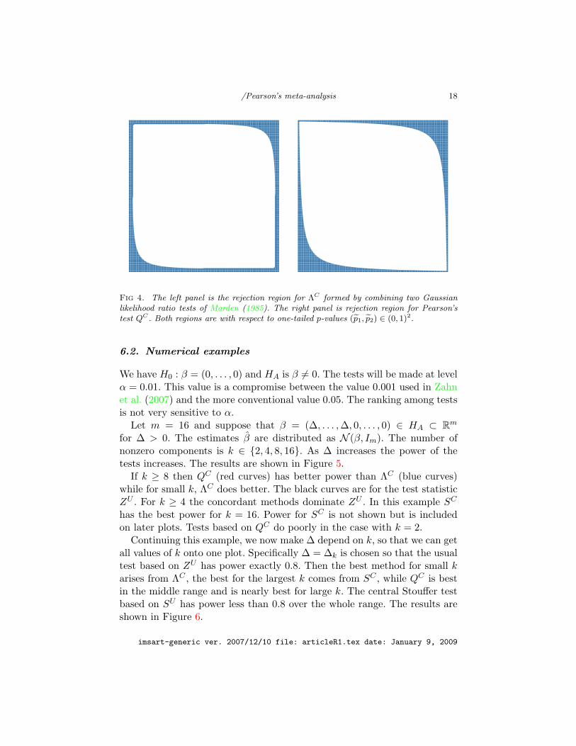
Figure 4 compares the rejection regions for ΛC and QC . Here we see thatQC has more of its rejection region devoted to coordinated alternatives thandoes ΛC . Recalling Figure 2 we note that SC has even more of its regiondevoted to coordinated alternatives than QC and so QC is in this senseintermediate between these two tests.

Marden (1985) also presents an LRTS based on t-statistics. As the degreesof freedom increase the t statistics rapidly approach the normal case consid-ered here. They are not however an exponential family at finite degrees offreedom. If experiment j gives a t statistic of Tj on nj degrees of freedom,then the one-sided likelihood ratio test rejects H0 for large values of

TR =m∑

j=1

(nj + 1) log(1 + max(Tj , 0)2/nj). (6.1)

This is equation (18) of Marden (1985), after correcting a small typograph-ical error. For large n the summands in (6.1) expressed as functions ofpj ∼ U(0, 1) are very similar to max(0, Zj)2.



Fig 4. The left panel is the rejection region for ΛC formed by combining two Gaussianlikelihood ratio tests of Marden (1985). The right panel is rejection region for Pearson’stest QC . Both regions are with respect to one-tailed p-values (p1, p2) ∈ (0, 1)2.

6.2. Numerical examples

We have H0 : β = (0, . . . , 0) and HA is β 6= 0. The tests will be made at levelα = 0.01. This value is a compromise between the value 0.001 used in Zahnet al. (2007) and the more conventional value 0.05. The ranking among testsis not very sensitive to α.

Let m = 16 and suppose that β = (∆, . . . ,∆, 0, . . . , 0) ∈ HA ⊂ Rm

for ∆ > 0. The estimates β are distributed as N (β, Im). The number ofnonzero components is k ∈ {2, 4, 8, 16}. As ∆ increases the power of thetests increases. The results are shown in Figure 5.

If k ≥ 8 then QC (red curves) has better power than ΛC (blue curves)while for small k, ΛC does better. The black curves are for the test statisticZU . For k ≥ 4 the concordant methods dominate ZU . In this example SC

has the best power for k = 16. Power for SC is not shown but is includedon later plots. Tests based on QC do poorly in the case with k = 2.

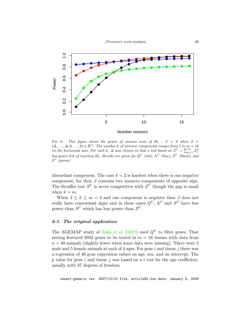
Continuing this example, we now make ∆ depend on k, so that we can getall values of k onto one plot. Specifically ∆ = ∆k is chosen so that the usualtest based on ZU has power exactly 0.8. Then the best method for small karises from ΛC , the best for the largest k comes from SC , while QC is bestin the middle range and is nearly best for large k. The central Stouffer testbased on SU has power less than 0.8 over the whole range. The results areshown in Figure 6.



0 1 2 3 4 5

0.0

0.2

0.4

0.6

0.8

1.0

Delta

Pow

er16 8 4 2

Fig 5. This figure shows power ranging from near 0 to 1 for a test of H0 at level α = 0.01.The alternative hypothesis is HA. The true parameter values β have k components ∆ > 0and m− k components 0. Here m = 16 and the values of k are printed above their powercurves. The black lines are for the usual χ2 test statistic ZU =

∑jZ2

j . The red lines are

for QC and the blue lines are for ΛC . For each curve, upper and lower bounds are plotted,but they almost overlap.

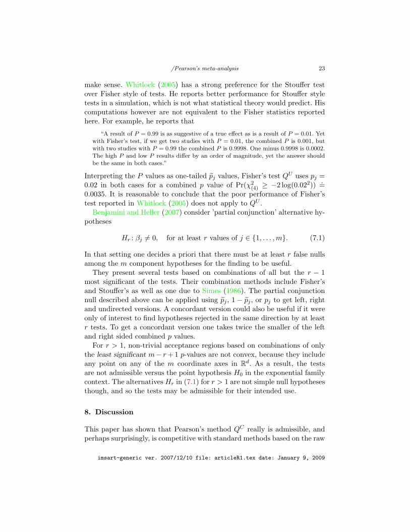
Finally, we consider the setting where k − 1 of the βj equal to ∆k > 0while one of them is −∆k. Again ∆k is chosen so that a test based on ZU

has power 0.8. Figure 7 shows the results. For small k ΛC works best, whilefor larger k, QC works best. The Stouffer test SC is best when k = 16, butloses power quickly as k decreases.

An online supplement at http://stat.stanford.edu/∼owen/reports/KPearsonSupplement contains 32 plots like the figures shown here. The casesconsidered have m ∈ {4, 8, 12, 16}, α ∈ {0.01, 0.05}, and power in {0.8, 0.5}.The number k of nonzero components ranges from 1 to m. In one set of plotsthere are k positive components, while the other has k − 1 positive and 1negative component.

Those other figures show the same patterns as the one highlighted here.Among the concordant tests ΛC is best for small k, then QC is best formedium sized k, and finally SC is best for the largest k. When there is onenegative component, SC is most adversely affected and ΛC least. That is, thetests that gain the most from coordinated alternatives, lose the most from a


http://stat.stanford.edu/~owen/reports/KPearsonSupplement

http://stat.stanford.edu/~owen/reports/KPearsonSupplement


5 10 15

0.0

0.2

0.4

0.6

0.8

1.0

Number nonzero

Pow

er

●

●

●●

●● ● ● ● ● ● ● ● ● ● ●

●

●

●●

●● ● ● ● ● ● ● ● ● ● ●

● ● ● ● ● ● ● ● ● ● ● ● ● ● ● ●

● ● ● ● ● ● ● ● ● ● ● ● ● ● ● ●

●

●

●

●

●

●

●

●●

●● ● ● ● ● ●

●

●

●

●

●

●

●

●●

●● ● ● ● ● ●

●

●

●

●●

●● ● ● ● ● ● ● ● ● ●

●

●

●

●●

●● ● ● ● ● ● ● ● ● ●

Fig 6. This figure shows the power of various tests of H0 : β = 0 when β =(∆, . . . , ∆, 0, . . . , 0) ∈ Rm. The number k of nonzero components ranges from 1 to m = 16on the horizontal axis. For each k, ∆ was chosen so that a test based on ZU =

∑m

j=1Z2

j

has power 0.8 of rejecting H0. Results are given for QC (red), ΛC (blue), SC (black), andSU (green).

discordant component. The case k = 2 is hardest when there is one negativecomponent, for then β contains two nonzero components of opposite sign.The Stouffer test SU is never competitive with ZU though the gap is smallwhen k = m.

When 2 ≤ k ≤ m = 4 and one component is negative then β does notreally have concordant signs and in these cases QC , ΛC and SC have lesspower than SU which has less power than ZU .

6.3. The original application

The AGEMAP study of Zahn et al. (2007) used QC to filter genes. Thatsetting featured 8932 genes to be tested in m = 16 tissues with data fromn = 40 animals (slightly fewer when some data were missing). There were 5male and 5 female animals at each of 4 ages. For gene i and tissue j there wasa regression of 40 gene expression values on age, sex, and an intercept. Thep value for gene i and tissue j was based on a t test for the age coefficient,usually with 37 degrees of freedom.



5 10 15

0.0

0.2

0.4

0.6

0.8

1.0

Number nonzero

Pow

er

●

●

●

●

●

●

●●

●●

● ● ● ● ● ●

●

●

●

●

●

●

●●

●●

● ● ● ● ● ●

●

●●

●●

●●

● ● ● ● ● ● ● ● ●

●

●●

●●

●●

● ● ● ● ● ● ● ● ●

●

●●

●

●

●

●

●

●

●

●●

●● ● ●

●

●●

●

●

●

●

●

●

●

●●

●● ● ●

●

●

●

●●

●● ● ● ● ● ● ● ● ● ●

●

●

●

●●

●● ● ● ● ● ● ● ● ● ●

Fig 7. This figure shows the power of various tests of H0 : β = 0 when β =(−∆, ∆, . . . , ∆, 0, . . . , 0) ∈ Rm. The number k of nonzero components ranges from 1 tom = 16 on the horizontal axis. There is always one negative component. For each k, ∆was chosen so that a test based on ZU =

∑m

j=1Z2

j has power 0.8 of rejecting H0. Results

are given for QC (red), ΛC (blue), SC (black), and SU (green). In this figure Monte Carlowas used for QC and ΛC .

Of the 16 tissues investigated, only 9 appeared to show any aging, and somuch of the analysis was done for just those 9.

The biological context made it impossible to specify a single alternativehypothesis, such as HL, HR or HL ∪ HR to use for all genes. Instead itwas necessary to screen for interesting genes without complete knowledgeof which tissues would behave similarly. Also, the fates of tissues differ inways that were not all known beforehand. One relevant difference is thatthe thymus involutes (becomes fatty) while some other tissues become morefibrous. There are likely to be other differences yet to be discovered thatcould make one tissue age differently from others.

The 8932 genes on any given microarray in the study were correlated.There were also (small) correlations between genes measured in two dif-ferent tissues for the same animal. It is of course awkward to model thecorrelations among an 8932 × 16 matrix of observations based on a sampleof only 40 such matrices. An extensive simulation was conducted in Owen(2007). In that simulation genes were given known slopes and then errors



were constructed by resampling residual matrices for the 40 animals. Byresampling residuals, some correlations among genes and tissues were re-tained. In each Monte Carlo sample, the genes were ranked by all the tests,and ROC curves described which test method was most accurate at rankingthe truly age-related genes ahead of the others.

In that Monte Carlo simulation, there were k ∈ {3, 5, 7} nonzero slopesout of m ∈ {9, 16}. Various values of ∆ were used. The Fisher based testsconsistently outperformed Stouffer style tests, as statistical theory wouldpredict. The concordant tests usually outperformed central tests, and werealmost as good as the one-sided tests that we would use if we knew thecommon sign of the nonzero βj . The exceptions were for cases with k = 3and m = 16 and large ∆. Then the QU tests could beat the QC tests. Fork = 3 and m = 16 and small ∆ the undirected and concordant tests wereclose. The left side of Figure 6 confirms that pattern.

6.4. Power conclusions

The methods of this section can be used to compare different combinationsof tests. Given precise information, such as a prior distribution π(β) for non-null β, one could employ a weighted sum of power calculations to estimate∫Rm π(β) Pr(Q ≥ Q1−α | β)dβ for each test Q in a set of candidates.Given less precise qualitative information, that the alternatives are likely

to be concordant, we can still make a rough ordering of the methods whenwe have some idea how many concordant non-null hypotheses there maybe. Of the concordant methods compared above, the LRT ΛC is best wherethere are a few concordant non-nulls, then Pearson’s QC is best if we expectmostly concordant non-nulls, and finally Stouffer’s method SC came outbest only when the concordant non-nulls were unanimous or nearly so.

7. Recent literature

Although combination of p-values is a very old subject, there seems to bea revival of interest. Here, a few works related to the present setup areoutlined.

Whitlock (2005) takes the strong view that any discordant test means thatthe null hypothesis should not be rejected. He gives the example of inbredanimals being significantly larger than outbred in one study but significantlysmaller in another study, and says that the results should then cancel eachother out. In some contexts, such as AGEMAP, such cancellation would not



make sense. Whitlock (2005) has a strong preference for the Stouffer testover Fisher style of tests. He reports better performance for Stouffer styletests in a simulation, which is not what statistical theory would predict. Hiscomputations however are not equivalent to the Fisher statistics reportedhere. For example, he reports that

“A result of P = 0.99 is as suggestive of a true effect as is a result of P = 0.01. Yetwith Fisher’s test, if we get two studies with P = 0.01, the combined P is 0.001, butwith two studies with P = 0.99 the combined P is 0.9998. One minus 0.9998 is 0.0002.The high P and low P results differ by an order of magnitude, yet the answer shouldbe the same in both cases.”

Interpreting the P values as one-tailed pj values, Fisher’s test QU uses pj =0.02 in both cases for a combined p value of Pr(χ2

(4) ≥ −2 log(0.022)) .=0.0035. It is reasonable to conclude that the poor performance of Fisher’stest reported in Whitlock (2005) does not apply to QU .

Benjamini and Heller (2007) consider ’partial conjunction’ alternative hy-potheses

Hr : βj 6= 0, for at least r values of j ∈ {1, . . . ,m}. (7.1)

In that setting one decides a priori that there must be at least r false nullsamong the m component hypotheses for the finding to be useful.

They present several tests based on combinations of all but the r − 1most significant of the tests. Their combination methods include Fisher’sand Stouffer’s as well as one due to Simes (1986). The partial conjunctionnull described above can be applied using pj , 1− pj , or pj to get left, rightand undirected versions. A concordant version could also be useful if it wereonly of interest to find hypotheses rejected in the same direction by at leastr tests. To get a concordant version one takes twice the smaller of the leftand right sided combined p values.

For r > 1, non-trivial acceptance regions based on combinations of onlythe least significant m− r + 1 p-values are not convex, because they includeany point on any of the m coordinate axes in Rd. As a result, the testsare not admissible versus the point hypothesis H0 in the exponential familycontext. The alternatives Hr in (7.1) for r > 1 are not simple null hypothesesthough, and so the tests may be admissible for their intended use.

8. Discussion

This paper has shown that Pearson’s method QC really is admissible, andperhaps surprisingly, is competitive with standard methods based on the raw



data, not just the p-values. The context where it is competitive is one wherethe truly nonzero components of the parameter vector are predominantly ofone sign. We have also studied a concordant LRT test ΛC which performswell when the number of concordant alternatives is slightly less.

Also a very simple Bonferroni calculation proved to be very accurate forfinding critical values of tests. It is less accurate for computing modest powerlevels.

In a screening setting like AGEMAP, we anticipate that noise artifactscould give rise to values βj with arbitrary patterns of signs, while the truebiology is likely to be dominated by concordant signs. In early stages of theinvestigation, false discoveries are considered more costly than false non-discoveries, because the former lead to lost effort. Later when the agingprocess is better understood, there may be greater value in finding thosegenes that are strongly discordant. In that case combination statistics whichfavor discordant alternatives may be preferred.

Finally, this work has uncovered numerous errors in earlier papers. I donot mean to leave the impression that the earlier workers were not careful,either in an absolute or relative sense. The subject matter is very slippery.

Appendix A: Computation

We want to get the 1 − α quantile of the distribution of Q =∑m

j=1 Yj

where Yj are independent but not necessarily identically distributed randomvariables on [0,∞). The case of random variables with a different lowerbound, possibly −∞ is considered in a remark below. We suppose that Yj

has cumulative distribution function Fj(y) = Pr(Yj ≤ y) which we cancompute for any value y ∈ [0,∞).

A.1. Convolutions and stochastic bounds

Because the Yj are independent, we may use convolutions to get the distri-bution of Q. Convolutions may be computed rapidly using the fast Fouriertransform. A very fast and scalable FFT is described in Frigo and Johnson(2005) who make their source code available. Their FFT on N points istuned for highly composite values of N (not just powers of 2) while costingat most O(N log(N)) time even for prime numbers N . Thus one does notneed to pad the input sequences with zeros.

There are several ways to apply convolutions to this problem. For a dis-cussion of statistical applications of the FFT, including convolutions of dis-tributions, see the monograph by Monahan (2001). The best known method



convolves the characteristic functions of the Yj to get that of Q and then in-verts that convolution. But that method brings aliasing problems. We preferto convolve probability mass functions. This replaces the aliasing problemby an overflow problem that is easier to account for.

We write F ⊗ G for the convolution of distribution functions F and G.Our goal is to approximate FQ = ⊗m

j=1Fj . We do this by bounding eachFj between a stochastically smaller discrete CDF F−

j and a stochasticallylarger one F+

j both defined below. Write F−j 4 Fj 4 F+

j for these stochasticinequalities. Then from

⊗mj=1F

−j 4 FQ 4 ⊗m

j=1F+j (A.1)

we can derive upper and lower limits for Pr(Q ≥ Q∗) for any specific valueof Q∗.

The support sets of F−j and F+

j are

Sη,N = {0, η, 2η, . . . , (N − 1)η} and S+η,N = Sη,N ∪ {∞}

respectively, for η > 0. The upper limit has

F+j (y) =

{Fj(y), y ∈ Sη,N

1, y = ∞.

In the upper limit, any mass between the points of S+η,N is pushed to the

right. For the lower limit, we push mass to the left. If Fj has no atoms inSη,N then

F−j (y) =

{Fj(y + η), y/η ∈ {0, 1, 2, . . . , N − 2}1, y = (N − 1)η

and otherwise we use limz↓(y+η) Fj(z) for the first N − 1 levels. We don’tneed to put mass at −∞ in F−

j because Fj has support on [0,∞).It should be more accurate to represent each Fj at values (i + 1/2)η for

0 ≤ i < N and convolve those approximations. See Monahan (2001). Butthat approach does not give hard upper and lower bounds for FQ.

Suppose that F and G both have support S+η,N with probability mass

functions f and g respectively. Then their convolution has support S+η,2N−1.

The mass at ∞ in the convolution is (f⊗g)(∞) = f(∞)+g(∞)−f(∞)g(∞).The mass at multiples 0 through 2N−2 times η, is the ordinary convolutionof mass functions f and g:

(f ⊗ g)(kη) =k∑

i=0

f(iη)g((k − i)η).



The CDF F ⊗G can then be obtained from the mass function f ⊗ g. Thusthe convolutions in (A.1) can all be computed by FFT with some additionalbookkeeping to account for the atom at +∞.

When F and G have probability stored at N consecutive integer multiplesof η > 0 then their convolution requires 2N − 1 such values. As a result thebounds in (A.1) require almost mN storage. If we have storage for only Nfinite atoms the convolution could overflow it. We can save storage by trun-cating the CDF to support S+

η,N taking care to round up when convolvingfactors of the upper bound and to round down when convolving factors ofthe lower bound.

For a CDF F with support S+η,M where M ≥ N define dF eN with support

S+η,N by

dF eN (iη) = F (iη), 0 ≤ i < N, and dF eN (∞) = 1.

That is, when rounding F up to dF eN , all the atoms of probability on Nηthrough (M − 1)η inclusive are added to the atom at +∞.

To round this F down to Sη,N we may take

bF cN (iη) = F (iη), 0 ≤ i < N − 1, and bF cN ((N − 1)η) = 1.

When rounding F down to bF cN , all the atoms on Nη through (M − 1)ηand +∞ are added to the atom at F ((N − 1)η). This form of roundingnever leaves an atom at +∞ in the stochastic lower bound for a CDF. Itis appropriate if the CDF being bounded is known to be proper. If theCDF to be bounded might possibly be improper with an atom at +∞ thenwe could instead move only the atoms of F on Nη through (M − 1)η tobF cN ((N − 1)η), leave some mass at ∞, and get a more accurate lowerbound.

The upper and lower bounds for FQ are now Fm+Q and Fm−

Q where

F j+Q = dF (j−1)+

Q ⊗ F+j eN , j = 1, . . . ,m,

F j−Q = bF (j−1)−

Q ⊗ F−j cN , j = 1, . . . ,m,

and F 0±Q is the CDF of a point mass at 0.

If all of the Fj are the same then one may speed things up further bycomputing F 2r+

1 via r− 1 FFTs in a repeated squaring sequence, and simi-larly for F 2r−

1 . For large m only O(log(m)) FFTs need be done to computeFm±

1 .



Remark 2. If one of the Fj has some support in (−∞, 0) then changes arerequired. If Fj has support [−Aj ,∞) for some Aj < ∞ then we can workwith the random variable Yj +Aj which has support [0,∞). The convolutionof Fj and Fk then has support starting at −(Aj + Ak). If Fj does not havea hard lower limit like Aj then we may adjoin an atom at −∞ to the CDFrepresenting its stochastic lower bound. As long as we never convolve adistribution with an atom at +∞ with another distribution having an atomat −∞, the results are well defined CDFs of extended real valued randomvariables.

A.2. Alternative hypotheses

In this section we get expressions for the CDFs Fj that need to be convolved.We suppose that βj are independent N (βj , 1) random variables for j =1, . . . ,m. The null hypothesis is H0 : β = 0 for β = (β1, . . . , βm).

The left, right, and undirected test statistics take the form∑m

j=1 Yj whereYj = t(βj) for a function t mapping R to [0,∞). Large values of Yj representstronger evidence against H0. The concordant test statistics are based onthe larger of the left and right sided sums.

The likelihood ratio tests ΛL, ΛR, and ΛU are sums of

YLj = max(−βj , 0)2, YRj = max(βj , 0)2 and YUj = β2j

respectively. After elementary manipulations, we find Fj for these tests via

Pr(YLj ≤ y) = Φ(√

y + βj), Pr(YRj ≤ y) = Φ(√

y − βj), andPr(YUj ≤ y) = Φ(

√y − βj)− Φ(−√y − βj).

The Fisher test statistics QL, QR, and QU are sums of

YLj = −2 log(Φ(βj)), YRj = −2 log(Φ(−βj)), and YUj = −2 log(2Φ(−|βj |),

respectively. The corresponding Fj are given by

Pr(YLj ≤ y) = Φ(βj − Φ−1(e−y/2)),

Pr(YRj ≤ y) = Φ(−βj − Φ−1(e−y/2)), and

Pr(YUj ≤ y) = Φ(βj − Φ−1

(12e−y/2

))− Φ

(βj + Φ−1

(12e−y/2

)).

For three of the Stouffer statistics, no FFT is required because SR ∼N (m−1/2 ∑m

j=1 βj , 1), SL = −SR, and SC = |SR|. The remaining Stoufferstatistic SU is the sum of YUj = |βj |/

√m, with

Pr(YUj ≤ y) = Φ(√

my − βj)− Φ(−√

my − βj).



A.3. Convolutions for power calculations

The computations for this paper were done via convolution using N =100,000 and η = 0.001. Some advantage might be gained by tuning N andη to each case, but this was not necessary. The convolution approach allowshard upper and lower bounds for probabilities of the form Pr(Q ≤ Q∗) forgiven distributions Fj . For practical values of N , the width of these boundsis dominated by discretization error in approximating F at N points. Empir-ically it decreases like O(1/N), for a given m, as we would expect becauseapart from some mass going to +∞, any mass being swept left or right,moves at most O(η/N). For very large values of N the numerical error inapproximating Φ−1 would become a factor.

Each convolution was coupled with a Monte Carlo computation of N sam-ple realizations. Partly this was done to provide a check on the convolutions.But in some instances the Monte Carlo answers were more accurate.

The possibility for Monte Carlo to be sharper than convolution arisesfor test statistics like QC = max(QR, QL). Suppose that QL and QR arenegatively associated and that we have bounds FL−

Q 4 FLQ 4 FL+

Q andFR−

Q 4 FRQ 4 FR+

Q . Even if FL−Q = FL+

Q and FR−Q = FR+

Q we still do notget arbitrarily narrow bounds for FC

Q . In particular, increasing N will notsuffice to get an indefinitely small interval.

When QL and QR are negatively associated then we can derive fromTheorem 2 that FC−

Q 4 FCQ 4 FC+

Q where for i = 0, . . . , N − 1,

FC−Q (iη) = FR−

Q (iη)FL−Q (iη),

FC+Q (iη) = max

(0, FR+

Q (iη) + FL+Q (iη)− 1

),

and FC+Q (∞) = 1.

Surprisingly, this is often enough to get a very sharp bound on QC . Butin some other cases the Monte Carlo bounds are sharper.

Monte Carlo confidence intervals for Pr(QC > Q∗) were computed by aformula for binomial confidence intervals in Agresti (2002, page 15). Thisformula is the usual Wald interval after adding pseudo-counts to the numberof successes and failures. For a 100(1− α)% confidence interval one uses

π ± Φ−1(1− α/2)√

π(1− π)/N

where π = (Nπ+Φ−1(1−α/2)2/2)/(N +Φ−1(1−α/2)2) and π is simply thefraction of times that QC > Q∗ was observed in N trials. For α = 0.001 this



amounts to adding Φ−1(.9995)2 .= 10.8 pseudo counts split equally betweensuccesses and failures, to the N observed counts.

Acknowledgments

I thank Stuart Kim and Jacob Zahn of Stanford’s department of Develop-mental Biology for many discussions about p values and microarrays thatshaped the ideas presented here. I thank Ingram Olkin for discussions aboutmeta-analysis and John Marden for comments on the likelihood ratio testsfor t-distributed data.

I thank two anonymous reviewers for their comments especially for men-tioning the article by Stein.

References

A. Agresti. Categorical data analysis. Wiley, New York, second edition,2002.

R. R. Bahadur. Rates of convergence of estimates and test statistics. Annalsof Mathematical Statistics, 38(2):303–324, 1967.

Y. Benjamini and R. Heller. Screening for partial conjunction hypotheses.Technical report, Tel Aviv University, Department of Statistics and OR,2007.

A. Birnbaum. Combining independent tests of significance. Journal of theAmerican Statistical Association, 49(267):559–574, 1954.

A. Birnbaum. Characterizations of complete classes of tests of some mul-tiparametric hypotheses, with applications to likelihood ratio tests. TheAnnals of Mathematical Statistics, 26(1):21–36, 1955.

S. Boyd and L. Vandeberghe. Convex Optimization. Cambridge UniversityPress, Cambridge, 2004.

F. N. David. On the Pλn test for randomness: remarks, futher illustration,and table of Pλn for given values of − log10(λn). Biometrika, 26(1/2):1–11,1934.

S. Dudoit and M. J. van der Laan. Multiple testing procedures with applica-tions to genetics. Springer-Verlag, New York, 2008.

J. D. Esary, F. Proschan, and D. W. Walkup. Association of random vari-ables, with applications. Annals of Mathematical Statistics, 38(5):1466–1474, 1967.

R. A. Fisher. Statistical Methods for Research Workers. Oliver and Boyd,Edinburgh, 4 edition, 1932.



M. Frigo and S. G. Johnson. The design and implementation of FFTW3.Proceedings of the IEEE, 93(2):216–231, 2005.

H. J. Greenberg and W. P. Pierskalla. A review of quasi-convex functions.Operations Research, 19(7):1553–1570, 1971.

L. Hedges and I. Olkin. Statistical methods for meta-analysis. AcademicPress, Orlando, FL, 1985.

J. I. Marden. Combining independent one-sided noncentral t or normal meantests. The Annals of Statistics, 13(4):1535–1553, 1985.

T. K. Matthes and D. R. Truax. Tests of composite hypotheses for themultivariate exponential family. The Annals of Mathematical Statistics,38(3):681–697, 1967.

J. F. Monahan. Numerical Methods of Statistics. Cambridge UniversityPress, Cambridge, 2001.

J. Oosterhoff. Combination of one-sided statistical tests. Mathematical Cen-ter Tracts, Amsterdam, 1969.

A. B. Owen. Pearson’s test in a large-scale multiple meta-analysis. Technicalreport, Stanford University, Department of Statistics, 2007.

E. S. Pearson. The probability integral transformation for testing goodnessof fit and combining independent tests of significance. Biometrika, 30(1):134–148, 1938.

K. Pearson. On a method of determining whether a sample of size n supposedto have been drawn from a parent population having a known probabilityintegral has probably been drawn at random. Biometrika, 25:379–410,1933.

K. Pearson. On a new method of deternining “goodness of fit”. Biometrika,26(4):425–442, 1934.

R. Simes. An improved Bonferroni procedure for multiple tests of signifi-cance. Biometrika, 73(3):751–754, 1986.

C. Stein. The admissibility of Hotelling’s t2-test. The Annals of Mathemat-ical Statistics, 27(3):616–623, 1956.

S. A. Stouffer, E. A. Suchman, L. C. DeVinney, S. A. Star, and R. M.Williams Jr. The American soldier,Volume I. Adjustment during Armylife. Princeton University Press, Princeton NJ, 1949.

L. H. C. Tippett. The method of statistics. Williams and Northgate, London,1931.

M.C. Whitlock. Combining probability from independent tests: the weightedZ-method is superior to Fisher’s approach. Journal of Evolutionary Biol-ogy, 18:1368–1373, 2005.

B. Wilkinson. A statistical consider ation in psychological research. Psy-chological Bulletin, 48:156–158, 1951.



J.M. Zahn, S. Poosala, A. B. Owen, D. K. Ingram, A. Lustig, A. Carter,A. T. Weeratna, D. D. Taub, M. Gorospe, K. Mazan-Mamczarz, E. G.Lakatta, K. R. Boheler, X. Xu, M. P. Mattson, G. Falco, Mi S. H. Ko,D. Schlessinger, J. Firman, S. K. Kummerfeld, W. H. Wood III, A. B.Zonderman, S. K. Kim, and K. G. Becker. AGEMAP: A gene expressiondatabase for aging in mice. PLOS Genetics, 3(11):2326–2337, 2007.


karl pearson's meta-analysis revisited - stanford...

Documents