juser.fz-juelich.de · metallischequasiteilchenfallenfürsupraleitendequbits: modellierung,...
TRANSCRIPT

Normal-Metal Quasiparticle TrapsFor Superconducting Qubits:
Modeling, Optimization, and ProximityEffect
Von der Fakultät für Mathematik, Informatik und Naturwissenschaftender RWTH Aachen University zur Erlangung des akademischen Grades
eines Doktors der Naturwissenschaften genehmigte Dissertation
vorgelegt von
Amin Hosseinkhani, M.Sc.aus Mashhad, Iran
Berichter: Universitätsprofessor Dr. David DiVincenzo,Universitätsprofessorin Dr. Kristel Michielsen
Tag der mündlichen Prüfung: March 01, 2018
Diese Dissertation ist auf den Internetseiten der Universitätsbibliothek online verfügbar.


Metallische Quasiteilchenfallen für supraleitende Qubits: Modellierung,Optimisierung, und Proximity-Effekt
Kurzfassung: Bogoliubov Quasiteilchen stören viele Abläufe in supraleitenden Elementen. Insupraleitenden Qubits wechselwirken diese Quasiteilchen beim Tunneln durch den Josephson-Kontakt mit dem Phasenfreiheitsgrad, was zu einer Relaxation des Qubits führt. Für Tempera-turen imMillikelvinbereich gibt es substantielle Hinweise für die Präsenz von Nichtgleichgewicht-squasiteilchen. Während deren Entstehung noch nicht einstimmig geklärt ist, besteht dennochdie Möglichkeit die von Quasiteilchen induzierte Relaxation einzudämmen indem man die Qu-asiteilchen von den aktiven Bereichen des Qubits fernhält. In dieser Doktorarbeit studieren wirQuasiteilchenfallen, welche durch einen Kontakt eines normalen Metalls (N) mit der supraleit-enden Elektrode (S) eines Qubits definiert sind. Wir entwickeln ein Modell, das den Einfluss derFalle auf die Quasiteilchendynamik beschreibt, wenn überschüssige Quasiteilchen in ein Trans-monqubit injiziert werden. Dieses Modell ermöglicht es, unter Berücksichtigung der Fallenpa-rameter die Zeitskala zu bestimmen, in der die überschüssigen Quasiteilchen aus dem Transmonevakuiert werden. Wir zeigen, dass die Evakuierungsdauer monoton mit der Fallengröße ansteigtund letztlich auf einen Grenzwert zuläuft, der von der Quasiteilchen-Diffusionskonstante undvon der Qubitgeometrie abhängt. Wir errechnen die charakteristische Fallengröße, bei welcherdieser Grenzwert erreicht wird. Wie es sich herausstellt, ist der limitierende Faktor für dieEinfangrate der Falle durch die langsame Quasiteilchenrelaxation im normalen Metall gegeben;diese Relaxation ist jedoch nur schwer kontrollierbar.
Um das Einfangen von Quasiteilchen zu optimieren, studieren wir den Einfluss von Größe,Anzahl und räumlicher Anordnung der Fallen. Diese Faktoren sind insbesondere wichtig, wenndie Falle die charakteristische Größe überschreitet. Wir diskutieren für einige experimentell rel-evante Beispiele wie die Evakuierungsdauer der überschüssigen Quasiteilchen optimiert werdenkann. Darüberhinaus zeigen wir, dass eine Falle nahe des Josephson-Kontaktes die stationäreQuasiteilchendichte an demselben Kontakt unterdrückt und den Einfluss von Fluktuationen derQuasiteilchenerzeugung reduziert.
Wenn metallische Elemente an ein supraleitendes Material gekoppelt sind, können Cooper-paare ins Metall entweichen. Mit dem Usadelformalismus greifen wir zunächst den Proximity-Effekt von gleichförmigen NS-Doppelschichten wieder auf; trotz der bereits langjährigen Er-forschung dieses Problems erlangen wir zu neuen Erkenntnissen über die Zustandsdichte. Wirverallgemeinern unsere Resultate danach für das ungleichförmige Problem in der Nähe der Fal-lenkante. Durch die Kombination dieser Resultate mit dem davor entwickelten Modell zurUnterdrückung der Quasiteilchendichte finden wir einen optimalen Abstand zwischen Falle undJosephson-Kontakt in einem Transmonqubit, welcher zu einer Minimierung der Qubitrelaxationführt. Dieser optimale Abstand, der die 4- bis 20-fache Kohärenzlänge beträgt, resultiert ausdem Wechselspiel zwischen Proximity-Effekt und Unterdrückung der Quasiteilchendichte. Wirschließen daraus, dass der schädliche Einfluss des Proximity-Effekts umgangen werden kannsolange die Entfernung zwischen Falle und Kontakt größer als der optimale Abstand ist.


Normal-Metal Quasiparticle Traps for Superconducting Qubits:Modeling, Optimization, and Proximity Effect
Abstract: Bogoliubov quasiparticle excitations are detrimental for the operation of many su-perconducting devices. In superconducting qubits, quasiparticles interact with the qubit degreeof freedom when tunneling through a Josephson junction, and this interaction can lead to qubitrelaxation. At millikelvin temperatures, there is substantial evidence of nonequilibrium quasi-particles. While there is no agreed upon explanation for the origin of these excess quasiparticles,it is nevertheless possible to limit the quasiparticle-induced relaxation by steering quasiparticlesaway from qubit active elements. In this thesis, we study quasiparticle traps that are formed bya normal-metal in tunnel contact with the superconducting electrode of a qubit. We develop amodel to explain how a trap can influence the dynamics of the excess quasiparticles injected ina transmon-type qubit. This model makes it possible to find the time it takes to evacuate theinjected quasiparticles from the transmon as a function of trap parameters. We show when thetrap size is increased, the evacuation time decreases monotonically and saturates at a level thatdepends on the quasiparticles diffusion constant and the qubit geometry. We find the charac-teristic trap size needed for the evacuation time to approach the saturation value. It turns outthat the bottleneck limiting the trapping rate is the slow quasiparticle energy relaxation insidethe normal-metal trap, a quantity that is very hard to control.
In order to optimize normal-metal quasiparticle trapping, we study the effects of trap size,number, and placement. These factors become important when the trap size increases beyondthe characteristic length. We discuss for some experimentally relevant examples how to shortenthe evacuation time of the excess quasiparticle density. Moreover, we show that a trap in thevicinity of a Josephson junction can significantly suppress the steady-state quasiparticle densitynear that junction and reduce the impact of fluctuations in the generation rate of quasiparticles.
When such normal-metal elements are connected to a superconducting material, Cooper-pairs can leak into the normal-metal trap. This modifies the superconductor properties and,in turn, affects the qubit coherence. Using the Usadel formalism, we first revisit the proximityeffect in uniform NS bilayers; despite the long history of this problem, we present novel findingsfor the density of states. We then extend our results to describe a non-uniform system in thevicinity of a trap edge. Using these results together with the previously developed model forthe suppression of the quasiparticle density due to the trap, we find in a transmon qubit anoptimum trap-junction distance at which the qubit relaxation rate is minimized. This optimumdistance, of the order of 4 to 20 coherence lengths, originates from the competition betweenproximity effect and quasiparticle density suppression. We conclude that the harmful influenceof the proximity effect can be avoided so long as the trap is farther away from the junction thanthis optimum.


AcknowledgementsBefore starting the main part of the thesis, I would like to take the opportunity to express mydeepest gratitude to several people who helped and supported me during my doctoral studies.First of all, I am greatly thankful to my PhD supervisor Dr. Gianluigi Catelani for his kindand constant support. I am indebted for countless enjoyable discussions with him during whichI learned to focus on Physics behind the mathematics. I also like to thank him for sending meto a lot of conferences and schools where I got a chance to expand my knowledge and to meetand discuss with a lot of physicists. I also enjoyed a lot by collaborating with experimentalscientists at Yale University, which was made possible by Gianluigi.
I am grateful to my friend Dr. Roman-Pascal Riwar for a lot of scientific as well as every-day-life discussions that we had. He also kindly helped me in translating the abstract of thisthesis into (Swiss) German.
I like to express my deep gratitude to Prof. David DiVincenzo for reviewing my thesis, hissupport for my postdoc applications, and the friendly and relaxed atmosphere at the JARA-Institute of Quantum Information. I would like to thank the second reviewer of my thesis Prof.Kristel Michielsen and also other members of my PhD committee, Prof. Thomas Schäpersand Prof. Christoph Stampfer, for the time they spent on reading my thesis and their fruitfulcomments.
I would also like to thank all of my colleagues in JARA-Institute of Quantum Informationat Forschungszentrum Jülich and RWTH Aachen University; few of which include Dr. DanielZeuch for a lot of discussions we had almost every day and also helping me in the Germanabstract of the thesis, Dr. Sbastian Mehl for helping me with a lot of paper works at the time Ijust had started my doctoral study in Germany, Alessandro Ciani for kindly preparing my PhDgraduation hat, and Alwin van Steensel for a lot of discussions and his kind PhD gift.
I like to particularly thank Dr. Mohammad H. Ansari for lots of interesting discussions thatwe had during my doctoral studies and also his kind support for my postdoc application to hisresearch group. I am very thankful to Ms. Luise Snyders who helped me very much for handlingofficial paper works at Forschungszentrum Jülich. I also like to thanks Ms. Helene Barton forhelping me in doing paper works at RWTH Aachen University.
I like to thank Dr. Hamed Saberi who supervised me during my Master’s program at ShahidBeheshti University, Tehran, Iran and supporting my PhD applications. I would like to thankProf. Ali Rezakhani for co-advising my master’s thesis and also for inviting me to visit Institutefor Research in Fundamental Sciences (IPM), Tehran, Iran in September 2016. I also thank Dr.Sahar Alipour for scheduling that visit.
I would like to thank Prof. Maksym Serbyn for inviting me to visit his group at Instituteof Science and Technology Austria in February 2018. I also like to thank Prof. Johannes Finkand Dr. Shabir Barzanjeh for a lot of interesting discussions that I had with them and theirhospitality during my visit to IST Austria.
I am thankful to Dr. Frank Deppe for inviting me to visit Walther-Meißner-Institute forLow-Temperature Research in March 2018. I greatly appreciate his hospitality and a lot ofinteresting discussions that we had.
I am grateful to Prof. Ahmad Ghodsi Mahmoudzadeh, my advisor during my bachelorstudies at Ferdowsi University of Mashhad, Iran, for his constant support and hospitality.

vi
I also like to thank all of my friends at Forschungszentrum Jülich whom I share a lot ofsweet memories: Esmaeel, Amin, Keyvan, Ali, Vahid, Masood and Davood. I like to especiallythank my friends at Aachen: Mojataba and his wife Shima, Alireza and his wife Zeinab, Sinaand Mehrdad. Our very nice memories made my life so colourful while I was living far from myfamily.
Finally and most importantly, I would like to express my deepest gratitude to my belovedparents who helped me at each second of my life. I am greatly thankful to my brother Yasinwho has always supported me in my life and my education. At the very last days of finalizingthis thesis, I was utterly joyed by born of my beloved nephew, Omid. I wish him all the best inhis life, and a happy family forever.

Contents
1 Introduction 11.1 Overview . . . . . . . . . . . . . . . . . . . . . . . . . . . . . . . . . . . . . . . . 11.2 Outline . . . . . . . . . . . . . . . . . . . . . . . . . . . . . . . . . . . . . . . . . 2
2 Quantum Coherent Superconducting Devices 52.1 Superconductivity . . . . . . . . . . . . . . . . . . . . . . . . . . . . . . . . . . . 5
2.1.1 Bogoliubov approach to BCS superconductivity . . . . . . . . . . . . . . . 62.1.2 Quasiparticle density in thermal equilibrium . . . . . . . . . . . . . . . . . 72.1.3 Superconducting gap . . . . . . . . . . . . . . . . . . . . . . . . . . . . . . 8
2.2 Josephson Effect . . . . . . . . . . . . . . . . . . . . . . . . . . . . . . . . . . . . 82.3 Superconducting Qubits . . . . . . . . . . . . . . . . . . . . . . . . . . . . . . . . 10
2.3.1 Cooper-pair box . . . . . . . . . . . . . . . . . . . . . . . . . . . . . . . . 102.3.2 Transmon qubit . . . . . . . . . . . . . . . . . . . . . . . . . . . . . . . . 13
2.4 Qubit-Quasiparticle Interaction . . . . . . . . . . . . . . . . . . . . . . . . . . . . 132.4.1 Energy relaxation induced by quasiparticle tunneling . . . . . . . . . . . . 14
3 Normal-Metal Quasiparticle Traps 193.1 Modeling . . . . . . . . . . . . . . . . . . . . . . . . . . . . . . . . . . . . . . . . 19
3.1.1 Introduction . . . . . . . . . . . . . . . . . . . . . . . . . . . . . . . . . . 193.1.2 The diffusion and trapping model . . . . . . . . . . . . . . . . . . . . . . . 203.1.3 Quasiparticle dynamics during injection and trapping . . . . . . . . . . . 243.1.4 Experimental data . . . . . . . . . . . . . . . . . . . . . . . . . . . . . . . 29
3.2 Optimization . . . . . . . . . . . . . . . . . . . . . . . . . . . . . . . . . . . . . . 323.2.1 Introduction . . . . . . . . . . . . . . . . . . . . . . . . . . . . . . . . . . 323.2.2 Enhancing the decay rate of the density . . . . . . . . . . . . . . . . . . . 333.2.3 Suppression of steady-state density and its fluctuations . . . . . . . . . . 40
3.3 Summary and Conclusions . . . . . . . . . . . . . . . . . . . . . . . . . . . . . . . 45
4 Quasiclassical Theory of Superconductivity 474.1 Gor’kov Equations . . . . . . . . . . . . . . . . . . . . . . . . . . . . . . . . . . . 474.2 Dyson Equation in Keldysh-Nambu Space . . . . . . . . . . . . . . . . . . . . . . 504.3 Eilenberger Equations . . . . . . . . . . . . . . . . . . . . . . . . . . . . . . . . . 524.4 The Dirty Limit . . . . . . . . . . . . . . . . . . . . . . . . . . . . . . . . . . . . 56
4.4.1 Boundary conditions for proximity systems . . . . . . . . . . . . . . . . . 584.4.2 Usadel equations for normal-superconducting hybrids . . . . . . . . . . . 59
5 Proximity Effect in Normal-Metal Quasiparticle Traps 615.1 Introduction . . . . . . . . . . . . . . . . . . . . . . . . . . . . . . . . . . . . . . . 615.2 Qubit relaxation due to quasiparticles . . . . . . . . . . . . . . . . . . . . . . . . 625.3 Proximity effect in thin films . . . . . . . . . . . . . . . . . . . . . . . . . . . . . 63
5.3.1 Uniform NS bilayers . . . . . . . . . . . . . . . . . . . . . . . . . . . . . . 63

viii Contents
5.3.2 Proximity effect near a trap edge . . . . . . . . . . . . . . . . . . . . . . . 665.4 Qubit relaxation with a trap near the junction . . . . . . . . . . . . . . . . . . . 70
5.4.1 Thermal equilibrium . . . . . . . . . . . . . . . . . . . . . . . . . . . . . . 705.4.2 Suppressed quasiparticle density . . . . . . . . . . . . . . . . . . . . . . . 72
5.5 Summary . . . . . . . . . . . . . . . . . . . . . . . . . . . . . . . . . . . . . . . . 77
6 Summary and Conclusions 79
A Tunneling rate equations 81
B Derivation of effective trapping rate 83B.1 Thin normal metal . . . . . . . . . . . . . . . . . . . . . . . . . . . . . . . . . . . 83B.2 Effective trapping rate . . . . . . . . . . . . . . . . . . . . . . . . . . . . . . . . . 85B.3 Effective trapping rate integrated over energy . . . . . . . . . . . . . . . . . . . . 87
C Comparison with vortex trapping 89
D Finite-size trap 91
E Quasi-degenerate modes and their observability 95
F Effective length 99F.1 Effective length due to the pad . . . . . . . . . . . . . . . . . . . . . . . . . . . . 99F.2 Effective length due to the gap capacitor . . . . . . . . . . . . . . . . . . . . . . . 100
G Quasiparticle Decay Rate and Steady-State Density 101G.1 Slowest Quasiparticle Decay Rate Due To Trap . . . . . . . . . . . . . . . . . . . 101
G.1.1 Single trap . . . . . . . . . . . . . . . . . . . . . . . . . . . . . . . . . . . 101G.1.2 Multiple side traps . . . . . . . . . . . . . . . . . . . . . . . . . . . . . . . 103
G.2 Suppression of Quasiparticle Steady-State Density . . . . . . . . . . . . . . . . . 105
H Traps in the Xmon geometry 107
I Proximity effect in uniform NS bilayers 109I.1 Weak-coupling limit . . . . . . . . . . . . . . . . . . . . . . . . . . . . . . . . . . 109I.2 Strong-coupling limit . . . . . . . . . . . . . . . . . . . . . . . . . . . . . . . . . . 111
J Numerical solution of the self-consistent equation for the order parameter 115
K Spatial evolution of single-particle density of states and pair amplitude 119
L Spectral function in the presence of a trap 123L.0.1 Thermal equilibrium . . . . . . . . . . . . . . . . . . . . . . . . . . . . . . 123L.0.2 Suppressed quasiparticle density . . . . . . . . . . . . . . . . . . . . . . . 125
Bibliography 127

Chapter 1
Introduction
1.1 Overview
In quantum world, a physical system can be in different eigenstates simultaneously. In partic-ular, one can imagine a quantum system in a superposition of two states,
|Ψ〉 = cos(θ
2
)|1〉+ sin
(θ
2
)eiφ|0〉, (1.1)
where we refer such quantum system as qubit; the qubit state can be conveniently illustrated bythe Bloch sphere drawn in figure (1.1). In 1994, Peter Shor devised a quantum algorithm runningon a set of qubits that enables to factorize an integer N to prime factors in an exponentiallyfaster time compared with classical algorithms using binary logic [1]. Such an algorithm can,for example, be used to break public key cryptography protocols. Since this discovery, therehas been extraordinary efforts to exploit the potentials of quantum systems for developingfuture technologies and also in finding physical systems promising to be controlled as a qubitand feasible to scale up. As any system interacts with its surrounding environment, a qubitthat is initially prepared in the superposition of two states will eventually decohere into amixed state that manifests itself in vanishing of the non-diagonal elements of qubit densitymatrix. In addition to qubit decoherence, faulty quantum preparation, faulty measurements andfaulty quantum gates impose an obstacle for realizing quantum computation. For these reasons,performing quantum error correction is at the heart of any scheme for realizing a universalquantum computer, that in turn requires the coherence time of physical qubits compared withgate time to exceed a threshold [2]. Further improvement of the qubit coherence above thethreshold is always favorable as it reduces the computational overhead due to quantum errorcorrection. Indeed, maintaining the qubit coherence, denoted by T2, for long enough times
Figure 1.1: Qubit state on a Bloch sphere. All points on the surface correspond to a superpo-sition between states |0〉 and |1〉.

2 Chapter 1. Introduction
is a key issue in all aspects of quantum technologies. There are generally two processes thatcontribute to the qubit decoherence. First, energy relaxation denoted by T1 that is an irreversibleprocess giving energy from or to the qubit which results in qubit state transition to the groundor excited state. Second, pure dephasing denoted by Tφ, is due to perturbations that do notinduce qubit state change, but randomly modulate the qubit phase. These two process combineto give,
1T2
= 12T1
+ 1Tφ. (1.2)
A large number of different systems have been proposed to realize physical qubits, each ofwhich utilize a specific physical property of the system to encode quantum information; forexample, intrinsic spin degree of freedom, photon polarization or phase difference across asuperconducting tunnel junction. Depending on what physical property is used to build a qubit,there are different decoherence mechanisms that are relevant for the system. In this thesis, weparticularly focus on superconducting qubits that are among the most promising candidates forrealization of quantum computation. There has been an extensive research in the community tocontrol and suppress various decoherence mechanisms leading to nearly six orders of magnitudeimprovement of coherence time in the past 20 years [3]. In particular, designing qubits thatoperate in a regime robust against charge noise [4, 5] together with improved understanding andcontrol of dielectric losses [6] and the Purcell effect [7] have made possible to reaching coherencetime more than 100µs. As the gate operation time for superconducting qubits is of order tensof nanoseconds [8], such long coherence time has enabled to perform about 104 operations pererror [3].
While the mentioned decoherence factors are imposed on the qubit from the surroundingenvironment, there is also an intrinsic decoherence channel that originates from the supercon-ductor itself: tunneling of unpaired electrons or quasiparticles across the Josephson junction.The theory of quasiparticle-induced decoherence is already developed and quasiparticle effectson relaxation, dephasing and parameter renormalization has been studied both theoretically[30, 31, 32, 33, 34, 35, 36, 37] and experimentally [18, 38, 39, 40, 41, 42, 43, 44, 45, 46]. Whilethe generation mechanism of non-equilibrium quasiparticles has yet remained a mystery in thefield, in this thesis we study ways to suppress quasiparticle density in order to minimize theirdetrimental effects. We illustrate how planting normal metals over some parts of the qubit cantrap quasiparticles and show how such trapping process can be optimized. Moreover, we studyinverse superconducting proximity effect and discuss how its detrimental consequences to thequbit operation can be avoided. While we mostly consider a 3D transmon qubit and give someconsideration of an Xmon qubit to explain and discuss our proposal, the idea of controllingquasiparticle population is also important in other superconducting devices such a Cooper-pairpumps, turnstiles and possible topological qubits based on Majorana zero modes where quasi-particle poisoning is a major obstacle. We therefore hope that our work will be of importanceand finds applications in those communities as well.
1.2 OutlineThe thesis is structured as follows: In chapter 2 we review the necessary backgrounds; section2.1 is devoted to remind the reader about formation of superconductivity and showing how

Chapter 1. Introduction 3
quasiparticles appear in the formalism. Section 2.2 uses perturbation theory to discuss about theJosephson effect. In section 2.3 we explain about two types of superconducting qubits, Cooper-pair box and transmon. We finally discuss in section 2.4 how quasiparticle tunneling resultsin qubit energy relaxation. Chapter 3 contains two sections that covers our published paperscited in references [47] and [68]. In section 3.1 we develop a phenomenological model governingthe dynamics and steady state density of quasiparticles. Considering a 3D-transmon qubit, thismodel allows one to evaluate the time it takes to evacuate the injected quasiparticles from thetransmon as a function of trap parameters. With the increase of the trap size, this time decreasesmonotonically, saturating at the level determined by the quasiparticles diffusion constant andthe qubit geometry. We determine the characteristic trap size needed for the evacuation time toapproach that saturation value. We also present experimental data (obtained by our colleagues)that support our theoretical findings. In section 3.2 we discuss how normal-metal quasiparticletraps can be optimized. We consider some experimentally relevant examples and find optimumtrap configurations that maximize the decay rate of excess quasiparticle density. Moreover, weshow that a trap in the vicinity of a Josephson junction can significantly reduce the steady-statequasiparticle density near that junction, thus suppressing the quasiparticle-induced relaxationrate of the qubit. Such a trap also reduces the impact of fluctuations in the generation rate ofquasiparticles, rendering the qubit more stable in time. We then turn our attention to studyhow a normal metal in contact with a superconductor can modify superconducting propertiesand what are the related consequences for the qubit coherence. In chapter 4, we review thequasicalssical theory of superconductivity in terms of Green’s functions in Keldysh-Nambu spaceand derive the Eilenberger equation. We then consider the dirty limit and derive the Usadelequation for a normal-superconducting hybrid that is our starting point to find the influence ofa normal-metal trap on the quasiparticle density of states. Chapter 5 contains our publishedpaper cited in reference [78]. Here, we first apply Usadel theory to a uniform bilayer and findnew analytical corrections to the density of states and minigap energy. We then consider a non-uniform hybrid relevant for physical realization of normal-metal trap for superconducting qubits.We find both theoretically and numerically the density of states and pair amplitude as a functionof distance from trap edge. Moreover, building on the phenomenological diffusion equation thatwe develop in chapter 3, we model the effect of the trap on the quasiparticle distributionfunction. This enables us to calculate different contributions to the qubit relaxation inducedby quasiparticle tunneling and pair processes. We find an optimum trap-junction distancethat minimizes the qubit relaxation rate. Placing the trap further from the junction thanthis optimum distance ensures that inverse proximity effect does not harm qubit coherence. Wesummarize and conclude our work in the last chapter. We have included a number of Appendicesas well that complement the main text and present some details of calculations.


Chapter 2
Quantum Coherent SuperconductingDevices
In this chapter we review the Bogoliubov approach to conventional superconductivity followedby discussing the Josephson effect and then two specific types of superconducting qubits,Cooper-pair box and transmon. We then consider qubit-quasiparticle interaction and presenthow quasiparticle tunneling results in qubit energy relaxation.
2.1 Superconductivity
Superconductivity was discovered in 1911 by H.K. Onnes when he witnessed electric resistanceof solid mercury suddenly dropping below any measurable value by cooling down to 4.2 K.Later, it was discovered by Meissner and Ochsenfeld that superconductors are diamagnets aswell [9] so that the electromagnetic field is expelled from a bulk superconductor beyond thematerial- and temperature-dependent penetration length. The microscopic explanation aboutsuperconductivity remained a challenge until 1957 when Bardeen, Cooper and Schrieffer pro-posed a model (BCS) that successfully explains this phenomenon [10]. The key idea of thismodel is that electrons condensate into a coherent state of pairs. The challenging question hereis how two electrons in a lattice can overcome the repulsive Coulomb interaction between them.This can be explained by taking into account the motion of ion cores or phonons; the first elec-tron polarizes its surrounding medium by attracting ion cores; the resulting positive ions canthen attract the second electron. While the importance of this electron-lattice interaction wasfirst pointed out in 1950 by Fröhlich [11], in 1956 Cooper showed however weak the (phonon-mediated) attractive interaction between two electrons is, the Fermi surface is unstable againstformation of a Cooper pair [12].
There are different approaches to BSC superconductivity, these include variational method,the Bogoliubov approach [13] and the Gor’kov approach [14]. The original BSC paper uses thevariational approach for which a trial wave function for the ground state of a superconductorup to the global phase is taken as:
|ΨBCS〉 =∏k
(|uk|+ eiφ|vk|c†k↑c†−k↓)|0〉 (2.1)
where c†kσ is the electron creation operator with momentum k and spin σ, |0〉 is the vacuum, theproduct is taken over all one-electron states and the coherence factors, uk and vk, are complexnumbers that satisfy normalization condition:
|uk|2 + |vk|2 = 1. (2.2)

6 Chapter 2. Quantum Coherent Superconducting Devices
Indeed, the BSC ground state is clearly a coherent superposition of all states with even numberof electrons from zero to infinity with an arbitrary phase factor eiφ.
The model Hamiltonian in BCS theory is,
HBCS =∑kσ
ξkc†kσc−kσ +
∑kk′
λkk′c†k↑c†−k↓c−k′↓ck′↑, (2.3)
in which, the energy ξk is measured from the Fermi energy. Since the attractive interaction ismediated by phonons, the coupling strength can be taken constant, λkk′ = −λ, when both thescattering-in and out electrons possess energies less than Debye frequency, |ξk|, |ξ′k| < ωD, andis zero otherwise. This model Hamiltonian describes the interaction between Cooper pairs andleads to formation of Cooper pair condensate as the ground state for a superconductor. The ideaof variational approach to BSC superconductivity is to minimize the expectation value of themodel Hamiltonian using the trial ground state given by Eq. (2.1). This enables us to find thecoherence factors in a straightforward calculation that we do not present here. Rather, in thissection we review the Bogoliubov approach that also gives the coherence factors and provides ahandy framework to deal with superconducting excitations as well. In chapter 4 we start fromGor’kov approach and present quasiclassical theory of superconductivity to study modificationsin superconducting properties when the superconductor is in proximity to a normal metal.
2.1.1 Bogoliubov approach to BCS superconductivity
To begin with, we note that since the ground state of a superconductor is formed from Cooperpair condensate including a macroscopic number of Cooper pairs, adding or removing an extraCooper pair does not really matter. In other words, the value for anomalous average definedas 〈c−k′↓ck′↑〉 is finite (averaging is taken with respect to the ground state of a superconductor)and fluctuations around this finite value are small . This enables us to arrive to the mean-fieldBCS Hamiltonian:
HMFBCS =
∑kσ
ξkc†kσc−kσ −
∑k
(∆c†k↑c†−k↓ + ∆∗c−k↓ck↑)−
|∆2|λ
. (2.4)
Here we only consider s-wave superconductivity where the order parameter is everywhere sym-metric in k space and is given by,
∆ =∑k′
λ〈c−k′↓ck′↑〉. (2.5)
We now introduce the Bogoliubov-quasiparticle operator defined as
γk↑ = u∗kck↑ + vkc†−k↓, (2.6)
γ−k↓ = −v∗kck↑ + ukc†−k↓, (2.7)
where the normalization condition for coherence factors, Eq. (2.2), is derived by enforcingfermionic anticommutation relations for Bogoliubov operators, γkσ, γ†k′σ′ = δσ,σ′δk,k′ .
The mean-field BCS Hamiltonian is diagonal in basis of Bogoliubov operators provided thefollowing relations for coherence factors hold,
|uk|2 = 12
(1 + ξk
εk
), (2.8a)
|vk|2 = 12
(1− ξk
εk
), (2.8b)

Chapter 2. Quantum Coherent Superconducting Devices 7
where
εk =√ξ2k + |∆2|. (2.9)
In finding these relations, it also turns out that the phase of superconducting order parameter∆ is equal to phase of vk relative to uk so that the order parameter has the same phase as theBSC ground state. The Hamiltonian then becomes,
HMFBCS = HG +Hqp, (2.10)
for which we defined,
HG =∑k
(ξk − εk)−|∆2|λ
, (2.11)
and,
Hqp =∑k
εk(γ†k↑γk↑ + γ†−k↓γ−k↓). (2.12)
Assuming a normal state at T = 0, we have ∆ = 0 and εk = |ξk|. The first term in Eq. (2.10)then differs from the corresponding one in the normal phase by,
HG −HNG (T = 0) = 2
∑k>kf
(ξk − εk)−|∆2|λ
. (2.13)
By changing the summation to an integration, it is easy to simplify this energy difference to−1
2N0|∆2| that is the condensation energy and expresses the energy gain by forming supercon-ductivity.
What is important for us is the second term in Eq. (2.10), Hqp, that illustrates the energyincrease corresponding to quasiparticle excitation above the Cooper pair condensate. Indeed,one can directly check from Eq. (2.1) that the superconducting ground state is vacuum state forquasiparticle excitations, γk|ΨBCS〉 = 0, that are gapped from the ground state condensate bythe value determined by the order parameter. Later in this chapter we will show that the densityof quasiparticle excitations has an important role in energy relaxation of superconducting qubits.In the following we find this density in thermal equilibrium.
2.1.2 Quasiparticle density in thermal equilibrium
The Bogoliubov transformation makes it clear that there is a one-to-one correspondence betweenelectronic and quasiparticle excitations. We can therefore write,
Nqp(ε)dε = Ne(ξ)dξ, (2.14)
where the quasiparticle density of states is denoted by Nqp(ε) and electronic density of statesby Ne(ξ). As we are interested in energies close to Fermi level, we take Ne(ξ) ' Ne(ξF ) ≡ N0and find the normalized quasiparticle density of states for a bulk superconductor,
n(ε) = Nqp(ε)N0
= dξ
dε= Re
[ε√
ε2 −∆2
]sgn(ε). (2.15)

8 Chapter 2. Quantum Coherent Superconducting Devices
In thermal equilibrium, we use Fermi-Dirac distribution function to find the density of quasi-particle excitations relative to Cooper pair density,
xeqqp = 2
N0∆
∫ ∞∆
Nqp(ε)f eq(ε)dε =
√2πT∆ e−∆/T . (2.16)
This predicts that the quasiparticle density can be arbitrarily suppressed by reducing the tem-perature and is essentially negligible if T ∆.
2.1.3 Superconducting gap
In order to find the superconducting energy gap, we use the Bogoliubov transformation andfind from Eq. (2.5),
∆ = λ∑k′
u∗k′vk′[〈γ−k′↓γ†−k′↓〉 − 〈γ
†−k′↓γ−k′↓〉
]. (2.17)
As Bogoliubov quasiparticles are fermionic excitations, their occupation probability is deter-mined by the usual Fermi-Dirac distribution so that we can write,
〈γ−k′↓γ†−k′↓〉 − 〈γ†−k′↓γ−k′↓〉 = 1− 2n(εk′) = tanh(εk′/2T ). (2.18)
We now change the summation in Eq. (2.17) to integration and given the coherence factors,Eqs. (2.8), we find
1λN0
=∫ ωD
0
1√ξ2 + ∆2 tanh(
√ξ2 + ∆2/2T )dξ. (2.19)
In the limit where temperature approaches zero, we find 1λN0
= sinh−1 ωD∆ that in the weak
coupling limit, λN0 1, results in,
∆ ' 2ωDe−1/λN0 ωD. (2.20)
This indicates that the superconducting order parameter cannot be derived by treating thecoupling strength in a perturbative way. We can alternatively express Eq. (2.19) in terms ofquasiparticle energy,
1λN0
=∫ √ω2
D−∆2
∆
1√ε2 −∆2
tanh(ε/2T )dε. (2.21)
We use this relation in chapter 5 to calculate the order parameter for a proximitized supercon-ductor relative to a bulk superconductor.
2.2 Josephson EffectIn a Josephson junction formed by two superconductors that are interrupted by an insulatingtunnel barrier, a supercurrent flows through the device even in absence of an external bias. Thisphenomenon is due to the phase difference between the two superconducting electrodes formingthe junction. In this subsection, we use perturbation theory to study the Josephson effect.

Chapter 2. Quantum Coherent Superconducting Devices 9
One can alternatively use quasiparticle bound states to find the same Josephson equations [15].Let us consider the following Hamiltonian that expresses single electron tunneling across thejunction,
HT = t∑m,n
∑σ
(c†RmσcLnσ +H.c.), (2.22)
where we assumed a constant tunneling matrix element t, and R and L are labeling right andleft sides of the junction, respectively. The electron tunneling operator in terms of Bogoliubovoperators reads,
c†RmσcLnσ =umunγR†nσγLmσ + vmvnγ
R†nσγ
Lmσe
i(φR−φL)
+ unvm(γR†n↓ γ
L†m↑ − γ
R†n↑ γ
L†m↓
)eiφR + umvn
(γRn↑γ
Lm↓ − γRn↓γLm↑
)e−iφL , (2.23)
where the coherence factors, u and v, are taken real as Eq. (2.23) explicitly accounts for thephase difference across the junction. As the ground state of a superconductor is vacuum statefor quasiparticles, the tunneling Hamiltonian results in zero expectation value.
However, the tunneling Hamiltonian taken to the second-order perturbation theory givenby,
H(2)T =
∑i
HT1εiHT , (2.24)
has a finite value in the ground states. Here εi is the energy of intermediate states and theHamiltonian has terms that transfer two electrons to the right, two to the left, and with nonet electron transfer. The latter leads to a constant value in the expectation value that has nophysical effect. The terms with a net transfer to the right gives,
〈H(2)T 〉 =− t2
∑n,m
〈ΨLBCS,ΨR
BCS|umvne−iφLγRn↑γ
R†n↑ γ
Lm↓γ
L†m↓ + γRn↓γ
R†n↓ γ
Lm↑γ
L†m↑
εLn + εRmunvme
iφR |ΨLBCS,ΨR
BCS〉
=− 2t2ei(φR−φL) ∑n,m
umvnunvm1
εLn + εRm
=− 2t2ei(φR−φL)NL0 N
R0
∫ ∞−∞
dξL∫ ∞−∞
dξR∆εL
∆εR
1εL + εR
=− 2t2∆ei(φR−φL)NL0 N
R0
∫ ∞−∞
dθL
∫ ∞−∞
dθR1
cosh θL + cosh θR=− 1
16gTgK
∆ei(φR−φL), (2.25)
where the final equality is obtained by change of variables u = (θL + θR)/2 and v = (θL− θR)/2in the last integral that, up to prefactors, results in complete elliptic integral of the first kindat zero, K(0) = π/2. Here, NL
0 and NR0 are the density of states per spin at the Fermi energy
of the left and right electrode, gT = 4πe2NL0 N
R0 t
2 is the junction conductance, gK = e2/2π isthe conductance quantum and we assumed equal gap for both sides of the junction.
A similar calculation for the net transfer to the left gives the complex conjugate of Eq. (2.25).The sum of these two terms give the energy gain by electron pair tunneling,
U = −EJ cosφ. (2.26)

10 Chapter 2. Quantum Coherent Superconducting Devices
for which EJ = 18gTgK
∆ is Josephson energy and φ = φR − φL is the phase difference across thejunction. This energy is associated with a supercurrent that is driven by the phase differenceacross the junction which reads,
IJ = 2πΦ0
∂U
∂φ= π
2∆egT sinφ, (2.27)
where Φ0 = h/2e denotes the superconducting flux quantum. As we have just shown, thissupercurrent solely originates from the phase difference between the ground states of the super-conducting leads; therefore, it is a dissipationless current. If an external voltage V is imposedto the junction, the phase difference evolves in time according to the AC-Josephson effect,
V = Φ02π
dφ
dt(2.28)
Hence, the inductance of the Josephson junction LJ has a non-linear relation with the phasedifference,
LJ = V/dIJdt
= 1π∆gT
1cosφ (2.29)
This non-linearity together with the ultra-low dissipation provided by superconductivity makesJosephson junctions promising candidates to build qubits.
2.3 Superconducting Qubits
In the previous section we ignored the fact that as supercurrent flows through the junction,charges build up on the islands of the junction and consequently Coulomb interactions becomeimportant as well. These repulsive interactions give another energy scale for the system thatis the charging energy. For a single electron transfer to the island, it becomes Ec = e2/2Cwhere C is the total capacitance that the island makes with the environment. Once we takeinto account the charging energy, it becomes clear the Josephson-junction-based devices can actlike an artificial atom, as we explain in the following. In this section, we consider two types ofsuperconducting qubits: Cooper-pair box and transmon qubit. The former is the earliest typeof the superconducting qubits while the latter was realized some years later and is one the mostpromising ones in terms of the coherence time and scalability. In writing the Hamiltonian of thequbit, for the moment we neglect the presence of quasiparticles while just trying to give a briefqualitative explanation of their effect. In the next section we explicitly consider quasiparticlesand study how their tunneling across the junction result in qubit energy relaxation.
2.3.1 Cooper-pair box
In a pioneering experiment by Nakamura and co-authors [16], the Cooper-pair box was thefirst superconducting device used to demonstrate quantum Rabi oscillations. As schematicallydepicted in the left panel of figure (2.1), this qubit simply consists of a Josephson junction whereone of its islands is used to store charges, and the other island is to provide these charges. Thereis also a gate electrode enabling to shift the electrostatic potential of the island with respect to

Chapter 2. Quantum Coherent Superconducting Devices 11
Figure 2.1: Left panel: Circuit diagram of a Cooper-pair box. The island is isolated by theJosephson junction and a capacitor. Tuning the gate voltage Vg enables us to control the numberof extra Cooper pairs on the island. This voltage is sensitive to fluctuations in the charges thatare surrounding the island. Right panel: Circuit diagram of a single-junction transmon qubit.The Junction is shunted by a large capacitance to increase the ration of EJ/EC that makes thequbit robust against the charge noise.
the bulk electrode in order to tune the number of charges on the island. The Hamiltonian ofthis qubit reads,
H = Ec(N −Ng)2 − EJ cos φ, (2.30)
where the operator N counts the number of single electrons that are tunneling-in or out of theisland,
N |N〉 = N |N〉, (2.31)
and is conjugate to the Josephson phase operator, [φ, N/2] = i. The offset charge Ng = CgVg/e
is a continuous variable expressing the polarization charge on the island induced by the gatevoltage Vg.
Important feature of this qubit is that the island is made small enough such that the acces-sible thermal energy at millikelvin temperatures (where the qubit is operating) is much smallerthan the charging energy, Ec kBT . Moreover, the charging energy also dominates the Joseph-son energy, Ec EJ ; in this condition, the number of extra charges on the island becomes awell defined variable. The qubit Hamiltonian in charge basis reads,
H =∑N
Ec(N −Ng)2|N〉〈N | − EJ2 (|N〉〈N + 2|+ |N + 2〉〈N |) . (2.32)
The charging energy as a function of the offset charge, Ng, gives a set of parabolas associatedwith single-electron charges, N , present at the island. On the other hand, the Josephson energyconnects the nearby charge states with the same parity. By tuning the gate voltage such thatthe offset charge is close to the values where these parabolas cross each other, only the twocrossing states remain important and the effective Hamiltonian become a 2 × 2 matrix. Inparticular, assuming initially there is no single electron present at the island, the qubit workingpoint is at Ng = 1 that results in qubit states to be in superposition of |N〉 and |N + 2〉 chargestates,
|0〉 = |N〉+ |N + 2〉2 , and |1〉 = |N〉 − |N + 2〉
2 , (2.33)

12 Chapter 2. Quantum Coherent Superconducting Devices
Figure 2.2: Energy diagram for the first two low-laying states with even and odd parity. Thezero point energy in each panel is chosen at the bottom of ground state and energies arenormalized to average energy E1 = 1
2(Eeven0 + Eodd1 ). Panel (a): for Cooper-pair box, whereEJ/EC 1, energy levels have high charge dispersion. The dashed line in the figure pointsthe offset charge at the qubit working point; any deviation from this point changes the qubitfrequency. In addition, a transition from even to odd charge states induced by a single electrontunneling destroys the qubit state that is a superposition of charge states with same parity.Panels (b) and (c): as the ratio of EJ/EC is increased, the energy levels become less sensitiveto the offset charge. Panel (d): in the transmon regime, where EJ/EC 1, the energy levelsbecome insensitive to the offset charge. Moreover, the even and odd charge sectors contributeequally to the qubit logical state.
while the qubit frequency becomes ω01 = EJ .
Panel (a) of figure (2.2) illustrates the eigenenergies of the two low-lying states for the evenand odd sectors of the qubit Hamiltonian, Eq. (2.32). The figure makes it clear that the Cooper-pair box sufferers from two major drawbacks that limit its coherence time: First, the high chargedispersion of the energy levels makes qubit vulnerable to the charge noise. Indeed, fluctuationsof the charges in the surrounding environment causes the offset charge deviate from the workingpoint; this in turn modulates the qubit frequency and leads to qubit dephasing. Second, as it isshown in Eq. (2.33), the qubit states consist of symmetric superposition of charge states with

Chapter 2. Quantum Coherent Superconducting Devices 13
equal parity; if an unpaired electron tunnels to the island, it poisons the device by changingthe charge parity that brings the qubit out of its computational subspace. These issues limitedcoherence time of the Cooper-pair box to about 10−9 s that is more than 5 orders of magnitudeless than the nowadays state-of-the-art qubits, [6, 17].
2.3.2 Transmon qubit
Reducing the charge dispersion makes the qubit frequency less sensitive to the charge noise.This can be achieved, for example, by going into the transmon regime where the ratio ofEJ/EC is large. In this case, the quantum fluctuations of the phase is relatively small, whilethe uncertainty of charge in the qubit state is significant. Going to this regime, however, wouldalso reduce the anharmonicity of the energy levels, but remarkably, while the charge dispersiondecreases exponentially in EJ/EC , the anharmonicity is suppressed algebraically with a slowpower law in EJ/EC [4]. Indeed, there is a range for the ratio between energy scales EJand EC for which the charge dispersion is flattened, rendering the qubit robust against chargenoise, while enough anharmonicity is kept, thus avoiding the excitation of higher-level states.As schematically illustrated in right panel of figure 2.1, in order to realize the high ratio ofEJ/EC , the junction in transmon qubit is shunted by a large capacitor; this lowers the totalcharging energy, EC , and makes EJ/EC large. Panel(d) of figure (2.2) shows the two energylevels of transmon qubit with even and odd charge parity, while panels (b) and (c) illustratethe crossover from charging regime to transmon regime. The picture clearly shows that as theratio of EJ/EC is increased, the total charge dispersion rapidly decreases. Therefore, the energydifference between states with different parities rapidly decreases as well. Indeed, in transmonqubit the logical state of the qubit contains two physical states with even and odd parity whilethe energy difference between these two states is given by [4],
ωmeo = ωmeo cos(πNg), (2.34)
where,
ωmeo = 4√
8ECEJ(−1)m√
2π
22m
m!
(8EJEC
) 2m+14
e−√
8EJ/EC , (2.35)
for which m = 0 for the logical qubit ground state and m = 1 for the excited states. Therefore,a transmon qubit is also less disturbed from single-electron tunneling because this does notbring the qubit out of its computational subspace.
2.4 Qubit-Quasiparticle InteractionSo far, in writing down the qubit Hamiltonian, we have neglected the quasiparticle excitations.This is because, as it follows from Eq. (2.16), the quasiparticle density is negligible at millikelvintemperatures where superconducting qubits are operating. However, a number of experimentsfirmly confirm that at low temperatures (below around 0.1 Tc for Aluminum) quasiparticlesfail to equilibrate with the environment and their density significantly exceeds the expectedequilibrium value [18, 19, 20, 21]. These excitations have a detrimental effect on the performanceof superconducting devices in a wide range of applications. To name a few, they limit thesensitivity of photon detectors in astronomy [22, 23] and cooling power of micro-refrigerators

14 Chapter 2. Quantum Coherent Superconducting Devices
[24, 25] and cause braiding errors in proposed Majorana-based quantum computation [26, 27,28, 29]. In superconducting qubits, it has been firmly established both theoretically [30, 31,32, 33, 34, 35, 36, 37] and experimentally [18, 38, 39, 40, 41, 42, 43, 44, 45] that quasiparticletunneling causes qubit energy decay and dephasing. In addition, the residual nonequlibriumquasiparticles result in qubit excited state population in excess of thermal equilibrium value[46]. In this section we take quasiparticles into account and discus how their tunneling acrossthe junction results in qubit energy relaxation.
The system Hamiltonian in presence of quasiparticles can be divided into three parts
H = Hq +Hqp +Hint, (2.36)
where Hq is the qubit Hamiltonian and the second term describes presence of quasiparticles onthe left and right superconducting leads,
Hqp =∑s=L,R
∑k,σ
Ekγs†k,σγ
sk,σ. (2.37)
The third term describes quasiparticle tunneling across the junction; from Eq. (2.23) we write,
Hint = H0int +Hp
int, (2.38)
where the single quasiparticle tunneling, H0int, and pair tunneling, Hp
int, read up to a globalphase factor,
H0int =t
∑k,k′,σ
(uLkuRk′eiφ/2 − vRk′vLk e−iφ/2)γL†kσγRk′σ + H.c. , (2.39)
Hpint =t
∑k,k′
[(uLk vRk′eiφ/2 + uRk′vLk e−iφ/2)γL†k↑ γ
R†k′↓
+(vRk′uLk e−iφ/2 + vLk uRk′e
iφ/2)γRk′↓γLk↑] + (L↔ R). (2.40)
2.4.1 Energy relaxation induced by quasiparticle tunneling
The tunneling Hamiltonian makes possible qubit state transition occurring by exchanging energywith the tunneling quasiparticle. Up to lowest order in tunneling amplitude t, the transitionfrom excited state, |1〉, to the ground state, |0〉, with qubit frequency ω10 is found using Fermi’sgolden rule
Γ10 = 2π〈〈∑λqp
|〈0, λqp|Hint|1, ηqp〉|2δ(Eλ,qp − Eη,qp − ω10)〉〉, (2.41)
where ηqp (λqp) is the initial (final) state of quasiparticles with energy Eη,qp (Eλ,qp). Thedouble angular brackets 〈〈...〉〉 denote averaging over initial quasiparticle states and the summa-tion is over all quasiparticle states. To calculate this rate, we note that the pair tunneling partof the interaction Hamiltonian, Hp
int, contains terms creating or annihilating two quasiparticles;this absorbs or releases energy by amount twice the superconducting gap.
On the other hand, superconducting qubits are designed such that the qubit frequency ismuch smaller than twice the gap, ωif 2∆, since this is necessary to avoid breaking Cooperpairs during qubit operation. Therefore, up to the leading order given by Fermi’s golden rule,

Chapter 2. Quantum Coherent Superconducting Devices 15
the pair tunneling part does not contribute in the transition rate due to energy conservation.Moreover, we assume low-temperature limit so that the characteristic energy of quasiparticles,δε, (that is proportional to temperature and is measured from the gap) is small compared withsuperconducting energy gap, δε ∆. This enables us to approximate the coherence factors,Eqs. (2.8), by uk ' vk′ ' 1/
√2 that in turn simplifies the single-quasiparticle tunneling to,
H0int = t
∑k,k′,σ
i sin φ2 γL†kσγ
Rk′σ + H.c. (2.42)
The transition rate then factorizes into terms that separately account for qubit dynamics andquasiparticle kinetics,
Γ10 = |〈0| sin φ2 |1〉|2Sqp(ω10) (2.43)
where the quasiparticle current spectral density becomes,
Sqp(ω) =2πt2〈〈∑k,k′,σ
∑λqp
|〈λqp|γL†kσγRk′σ + γR†k′σγ
Lkσ|ηqp〉|2δ(Eλ,qp − Eη,qp − ω)〉〉
=4πt2∑k,k′,σ
〈〈〈ηqp|γR†k′σγRk′σ|ηqp〉〈ηqp|γLkσγ
L†kσ |ηqp〉δ(Eλ,qp − Eη,qp − ω)〉〉
=32EJπ∆
∫ ∞∆
n(ε)n(ε+ ω)f(ε)[1− f(ε+ ω)]dε. (2.44)
Here we used 〈〈〈ηqp|γR†γR|ηqp〉〉〉 = f(εR), 〈〈〈ηqp|γLγL†|ηqp〉〉〉 = 1 − f(εL) and tookEλ,qp − Eη,qp = ELλ,qp + ERλ,qp − ELη,qp − ERη,qp = εL − εR.
The spectral density depends on the quasiparticle distribution function; assuming “cold”quasiparticles meaning their energy (or effective temperature) is small compared with qubitfrequency, δε ω, we can take 1 − f(ε + ω) ' 1 and n(ε + ω) =
√∆2ω . This simplifies the
spectral function and we find;
Sqp(ω) = 8EJπxqp
√2∆ω
(2.45)
where
xqp = 2∆
∫ ∞∆
n(ε)f(ε)dε, (2.46)
is the density of quasiparticles normalized to the Cooper-pair density.In thermal equilibrium this quantity is given by Eq. (2.16). However, we note that Eq. (2.45)
is valid for arbitrary distribution function provided δε is the smallest energy scale of the system.To find the qubit excitation rate, Γ01, one has to calculate Sqp(ω) for ω < 0 that is obtainedfrom Eq. (2.44) by replacing ε → ε − ω, ω → −ω; within our low-temperature assumption,in general we have S(−ω) S(ω) indicating that there is no quasiparticle with energy highenough to excite the qubit. Eq. (2.45) is of central importance in this thesis as it indicates thatthe qubit decay rate can be decreased by reducing the quasiparticle density near the Josephsonjunction.

16 Chapter 2. Quantum Coherent Superconducting Devices
Figure 2.3: Panel (a) is reproduced and slightly modified from Ref. [19]. It illustrates experimen-tal data points for the number of quasiparticles in a superconducting resonator and comparesexperimental findings with theoretical prediction in thermal equilibrium. At low temperaturesrelevant to the operation of superconducting qubits, the residual quasiparticle density is sig-nificantly higher than theory predictions. Panel (b) is reproduced from Ref. [43] and makes itclear that suppressing the quasiparticle density, that in this case is achieved in a 3D transmonqubit by cooling in magnetic field to generate vortices, can improve the qubit coherence times.It is difficult to control vortices and it is observed that a large number of them can negativelyinfluence qubit performance.
In figure (2.3) we have shown some experimental highlights about quasiparticles and theirimpact on the qubit decay rate. Panel (a) shows the measured quasiparticle density in a su-perconducting resonator as a function of temperature and reveals that the density saturateswhen temperature goes below ∼ 160 mK. While a detailed knowledge of the source that gener-ates nonequilibrium quasiparticles is eventually needed to solve quasiparticle-related problems,physicists have been looking for ways to suppress quasiparticle density that promises improvingthe qubit coherence. One proposal that has been recently realized is to cool down the qubitin a magnetic field that would generate vortices in the device. At the core of a vortex, super-conducting order parameter is suppressed, which makes it possible to trap quasiparticles- we

Chapter 2. Quantum Coherent Superconducting Devices 17
describe the trapping mechanism in detail in the next chapter. Panel (b) of figure 2.3 showsmeasured relaxation times for a 3D transmon qubit as a function of magnetic field. The strengthof magnetic field determines the number of generated vortices and, consequently, the level ofsuppression in the quasiparticle density. The plot makes it clear that up to some point in themagnetic field, vortices could improve the qubit coherence while for magnetic field above ' 200mG, the qubit performance is negatively affected. This behavior is attributed to the energydissipation that a large number of vortices can cause [43]. Moreover, it is difficult to controlthe vortex position. This has motivated us to study another method for suppressing quasipar-ticle density that enables us to control trap size and placement. In the next chapter, we willintroduce normal-metal quasiparticle traps and discuss how they work and how they can beoptimized by proper trap placement.


Chapter 3
Normal-Metal Quasiparticle Traps
We begin this chapter by explaining how a normal-metal connected to superconducting qubit canact as a sink for quasiparticles. Section 3.1 contains part of our work that has been publishedunder the title Normal-metal quasiparticle traps for superconducting qubits and cited in Ref.[47]. Here we develop a model for the effect of a single small trap on the dynamics of the excessquasiparticles injected in a transmon-type qubit. Section 3.2 containes a paper of the author thathas been published with title Optimal configurations for normal-metal traps in transmon qubitsand cited in Ref. [68]. Here we build on section 3.1 and discuss how quasiparticle trapping canbe optimized. We show proper trap design can increase the slowest decay rate of quasiparticleand at the same time suppress quasiparticle steady-state density and its fluctuations.
I co-authored Ref. [47] and contributed by discussing the model and experimental data,comparing simplified analytical results with exact numerics and preparing a number of sug-gested figures for the paper. I contributed to Ref. [68] by doing all of exact and numericalmodelings and their corresponding figures to demonstrate enhancing the decay rate of the ex-cess quasiparticle density as well as suppression of the quasiparticle steady-state density due tonormal-metal traps, comparing normal-metal traps on the pads with vortex trapping, and theanalysis of traps for Xmon qubits.
3.1 Modeling
3.1.1 Introduction
Ideal superconducting devices rely on dissipationless tunneling of Cooper pairs across a Joseph-son junction. For example, in a Cooper pair pump [48], the controlled transport of Cooper pairsacross two or more junctions can in principle make it possible to relate frequency and currentand hence enable metrological applications of such a device [49]. For quantum informationpurposes, the non-linear relation between the supercurrent and the phase difference across ajunction makes the junction an ideal non-linear element to build a qubit [50]. However, in addi-tion to the pairs tunneling, single-particle excitations known as quasiparticles can also tunnel.In the pumps this leads to “counting errors”, limiting the accuracy of the current-frequency re-lation [48, 49]. In qubits, quasiparticles interact with the phase degree of freedom, providing anunwanted channel for the qubit energy relaxation [32, 6]. While in many cases it is impossibleto prevent the creation of quasiparticles, one may keep them away from the Josephson junctionsby trapping. Evacuation of the quasiparticles from the vicinity of the junction provides a wayto extend the energy relaxation time (T1) in the steady state, and to restore the steady stateafter a perturbation, whether caused by qubit operation or some uncontrolled environmentaleffect.
Quasiparticle trapping has been explored for a long time, and various proposal exists onhow to implement such a trapping. For example, gap engineering takes advantage of the fact

20 Chapter 3. Normal-Metal Quasiparticle Traps
that quasiparticles accumulate in regions of lower gap to steer them into or away from certainparts of the device. Gap engineering was used successfully to limit quasiparticle “poisoning” ina Cooper pair transistor [51], while proved ineffective in a transmon qubit [52]. A vortex in asuperconducting film can also act as a well-localized trap, since the gap is completely suppressedat the vortex position. Trapping by vortices has been demonstrated [53, 54, 43, 55], but vortexmotion may induce an unwanted dissipation. An island of a normal metal in contact with thesuperconductor may also serve as a quasiparticles trap [25, 56]. In the limit of weak electrontunneling across the contact, the proximity effect is negligible. The quasiparticles tunneled intothe normal metal are trapped there upon losing their energy by phonon emission or inelasticelectron-electron scattering.
The majority of previous works concentrated on the control of a steady-state quasiparticlepopulation [49, 25, 56]. In contrast, we are interested in the effect of a normal-metal trapon the dynamics of the quasiparticle density. Traps accelerate the evacuation of the excessquasiparticles injected in a qubit in the process of its operation. Our main goal is to determinehow the characteristic time of the evacuation depends on the parameters of a small normal-metal island in contact with the superconducting qubit. The characteristic time shortens withthe increase of the trap size, saturating at a value dependent on the qubit geometry and thequasiparticle diffusion coefficient. The size at which a trap becomes effective depends on thecontact resistance, the energy relaxation rate in the normal-metal island, and the effectivetemperature of the quasiparticles. We develop a simple model allowing to evaluate the timeevolution of the quasiparticle density and find the characteristic evacuation time as a functionof the trap parameters. The model is validated by measurements of the qubit T1 relaxationtime performed on a series of transmons with normal-metal traps of various sizes.
This section is organized as follows: in Sec. 3.1.2 we develop a phenomenological quasiparticlediffusion and trapping model which includes the effect of a normal-metal trap. In Sec. 3.1.3 westudy the dynamics of the density during injection and trapping in a simple configuration, andin Sec. 3.1.4 we provide experimental data (obtained by our collaborators in Yale University)supporting our approach.
3.1.2 The diffusion and trapping model
Let us consider a quasiparticle trap made of a normal (N) metal covering part of a super-conducting (S) qubit. The contact between the two superconductor and the normal trap isprovided by an insulating (I) layer characterized by a small electron transmission coefficient.In order to relate the quasiparticle tunneling rate to the conductance of the contact, we use thetunneling Hamiltonian formalism applied to a model N -I-S system, see Fig. 3.1,
H = Hqp +HN +HT , (3.1)Hqp =
∑nσ
εnγ†nσγnσ , (3.2)
HN =∑mσ
ξmc†mσcmσ , (3.3)
HT = t√ΩNΩS
∑m,n,σ
(c†mσdnσ + d†nσcmσ
). (3.4)

Chapter 3. Normal-Metal Quasiparticle Traps 21
0
1
2
3
0 1
dN
dS
N
S
0
1
0 1 2
N
S
tr
r
esc()
Figure 3.1: Left: a small superconductor S of thickness dS separated from a normal metal Nof thickness dN by an insulating layer. Right: depiction of the processes leading to trapping:tunneling from S to N with rate Γtr and from N to S with rate Γesc(ε), and relaxation in Nwith rate Γr.
We denote with ΩN,S = A × dN,S the volumes of the N and S layers, respectively (A is thearea of interface, and dN,S are the layers thicknesses); c†mσ and d†nσ are the creation operatorsfor electrons in the normal metal (energy ξm and spin σ) and superconductor. The electronoperators in the superconductor are related by Bogoliubov’s transformation to the quasiparticleannihilation (creation) operators γ(†)
nσ ,
dn↑ = unγn↑ + vnγ†n↓ (3.5)
d†n↓ = −vnγn↑ + unγ†n↓ (3.6)
u2n = 1− v2
n = 12
(1 + ξn
εn
). (3.7)
Here εn =√ξ2n + ∆2 is the energy of a quasiparticle, and ξn is the energy of electron in the
normal state of the superconductor. The tunneling constant t can be related, by Fermi’s goldenrule, to the resistance RT of the contact,
Rq2πRT
= 4π∣∣∣t∣∣∣2 νS0νN0 , Rq = 2π~
e2 , (3.8)
where νN0 and νS0 are the densities of states in the normal metal and in the (normal state ofthe) superconductor, respectively. The tunnel conductance, 1/RT , is proportional to the areaA of the junction; the intensive quantity characterizing the insulating layer is its conductanceper unit area, 1/RTA.
We may use Fermi’s golden rule to evaluate also the rates of tunneling-induced changeof the occupation factors of electrons, f(ξm) =
∑σ〈c†mσcmσ〉, and quasiparticles, fqp(εn) =∑
σ〈γ†nσγnσ〉. We can distinguish two processes. Quasiparticles tunnel from the superconductorinto the normal metal with rate Γtr = 2π
∣∣∣t∣∣∣2 νN0/ΩS . The transition rate is proportional to thedensity of the final states involved in the transition, therefore the quasiparticle trapping rate doesnot have a pronounced energy dependence. The complementary process of a non-equilibriumelectron escape into the superconductor, however, does display a strong energy dependence

22 Chapter 3. Normal-Metal Quasiparticle Traps
associated with the BCS singularity in the density of final states, Γesc (ε) = 2π∣∣∣t∣∣∣2 νS0νS(ε)/ΩN ;
hereνS(ε) = ε√
ε2 −∆2(3.9)
is the normalized BCS density of states.One can see from Eq. (3.8) that the rates Γtr and Γesc (ε) are independent of the area A at
fixed conductance per unit area of the insulating layer. We may express the rates as
Γtr = γtr/dS , Γesc(ε) = γesc(ε)/dN (3.10)
in terms of quantities independent of geometry, γtr and γesc,
γtr = Rq4π(RTA)νS0
, γesc = RqνS(ε)4π(RTA)νN0
. (3.11)
with (RTA) being the contact resistance times the area of the contact. This product, withunits of Ω·cm2, is independent of A, being inversely proportional to the transmission coefficientthrough the insulating barrier.
The above formulas enable us to estimate the trapping and escape rates for an aluminum-copper interface for a typical experimental setup (cf. Sec. 3.1.4): aluminum has a density ofstates νS0 = 0.73 × 1047/Jm3 [57] and a direct measurement of the contact resistance yields(RTA) ∼ 430 Ωµm2 (this corresponds to the transmission coefficient of order 10−5). TakingdS ∼ 80nm we find, using Eqs. (3.10) and (3.11), Γtr ∼ 8× 10⁶ s−1. The escape rate saturatesat an energy-independent value, Γesc(ε)→ Γesc at energies ε ∆. Since dS ≈ dN and νS0 ≈ νN0in a typical experiment, one has Γesc ≈ Γtr.
In writing the rate equations for the energy distribution functions of electrons and quasi-particles, we assume the continuum limit for energies ξm and εn. It is convenient to definethe probability density to find an electron (quasiparticle) in the normal metal (superconductor)with energy ε ≥ ∆ as
pN (ε) =νN0ΩN
νS0ΩSf(ε) (3.12)
pS(ε) =νS(ε)fqp(ε) . (3.13)
Without loss of generality, we normalize the probability with respect to νS0ΩS . Note thateventually, the experimentally accessible quantity is the normalized quasiparticle density, whichcan be derived from pS as
xqp = 2∆
∫ ∞∆
dε pS(ε) . (3.14)
In the absence of spatial dispersion of the distribution functions, the rate equations read (seeAppendix A)
pN (ε) =ΓtrpS (ε)− Γesc (ε) pN (ε)− ΓrpN (ε) , (3.15)pS (ε) =Γesc (ε) pN (ε)− ΓtrpS (ε) . (3.16)
The terms proportional to Γtr describe trapping of quasiparticle excitations in the normal metal,and those proportional to Γesc(ε) the possible escape of electron excitations back to the super-conductor; these events take place with rates described by Eqs. (3.10)-(3.11).

Chapter 3. Normal-Metal Quasiparticle Traps 23
Since the tunneling process is elastic, excitations appear in the normal metal at energiesclose to the gap ∆. At low temperature T ∆, there are many unoccupied states below ∆ inthe normal metal, into which the excitations can decay. These inelastic processes are mediatedby electron-electron and electron-phonon interactions and lead to relaxation, which we capturein Eq. (3.15) with the phenomenological rate Γr. All the processes included in the rate equations(3.15)-(3.16) are represented in the right panel of Fig. 3.1.
If the relaxation is immediate, the quasiparticles get trapped in the normal metal with rateΓtr. However, the relaxation rate Γr due to electron-electron and electron-phonon interactionsin the normal metal is of course finite. It has been estimated in the supplementary to [43] tobe Γr ∼ 107 s−1; the measurements reported in Ref. [58] lead to a relaxation rate for electron-phonon interaction of the same order of magnitude, while an estimate based on [59] yields thefaster relaxation rate Γr ∼ 108 s−1. In all cases, relaxation cannot be assumed immediate incomparison with the trapping and escape rates estimated above, especially taking into accountthat the escape rate quickly increases for energies approaching the gap due to the divergentBCS density of states in Eq. (3.9). In fact, for some energy interval close to the gap, the escaperate dominates the quasiparticle dynamics, such that the excitations do not have enough timeto relax. Therefore, we cannot in general neglect the backflow of excitations from the normaltrap to the superconductor.
The backflow may result in an effective rate which is slower than Γtr. Assuming a steady-state distribution of non-equilibrium electrons in the normal layer, we set pN = 0 in Eq. (3.15)and solve for pN in terms of pS (see also Appendix B). Substituting the solution into Eq. (3.16)and integrating over energy, we arrive at
xqp = −Γeffxqp , (3.17)
with the effective trapping rate defined by
Γeff = 1∫∞∆ dε pS(ε)
∫ ∞∆
dεΓtrΓr
Γesc(ε) + ΓrpS(ε) . (3.18)
It is clear that Γeff is suppressed to a level below Γtr. The level of suppression depends onthe typical width of the quasiparticle distribution function in energy space. Assuming pS(ε) ischaracterized by an effective temperature, T ∆, we find that the trapping is not suppressed,Γeff ≈ Γtr, only if the energy relaxation is fast enough (Γr (∆/T )1/2Γesc); in this caseexcitations in the normal metal quickly relax to energies below the gap and cannot returninto the superconductor. In the opposite case (Γr . (∆/T )1/2Γesc), the effective rate becomesT -dependent and suppressed below the nominal trapping rate, Γeff ≈ (2T/π∆)1/2ΓtrΓr/Γesc.Note that in the slow relaxation regime the effective trapping rate Γeff is independent of thetunneling probability between superconductor and normal metal, the limiting value of Γeff beingproportional to the relaxation rate.
The quasi-static approximation (pN = 0) we used above becomes justified once we movefrom the model system of Fig. 3.1 to a more realistic geometry of a long superconducting stripin contact with a metallic trap, see Fig. 3.2a. In that geometry, the time variation of thequasiparticle distribution function pS is controlled by the diffusion time in the strip, whichis typically substantially longer than 1/Γr. The generalization of the rate equations (3.15)and (3.16) to include diffusion is performed in Appendix B. In addition to diffusion, otherprocesses such as quasiparticle recombination, generation, and trapping in the bulk must be

24 Chapter 3. Normal-Metal Quasiparticle Traps
generally taken into account. For sufficiently thin normal and superconducting layers, we finda generalized diffusion equation for the quasiparticle density xqp,
xqp =Dqp∇2xqp − a(x, y)Γeffxqp − rx2qp − sbxqp + g , (3.19)
where xqp(x, y) depends only on coordinates in the plane of the superconducting strip (and isassumed constant across its thickness) and the area function a(x, y) equals 1 for x and y wherethe trap and the superconductor are in contact, and 0 elsewhere, see Fig. 3.2(a).
The diffusion constant Dqp in Eq. (3.19) is proportional to the normal-state diffusion con-stant for the electrons in the superconductor – the proportionality coefficient can in principlebe calculated from the detailed information on the energy distribution of quasiparticles that wediscard in using the phenomenological Eq. (3.19). The recombination term rx2
qp accounts forprocesses in which two quasiparticles recombine into a Cooper pair [60], again neglecting thedetails of the quasiparticle distribution. The relationship between recombination time, quasi-particle energy, and electron-phonon interaction strength can be found in [61]. Moreover, thereis a background trapping term sbxqp that describes any process that can localize a quasiparticleand hence remove its contribution to the bulk density xqp. Trapping by vortices is an exampleof such a process, recently characterized in [43]. The generation rate g describes pair-breakingprocesses, both thermal and non-thermal; at low temperatures, non-equilibrium processes ofunknown origin lead to a quasiparticle density orders of magnitude larger than the thermalequilibrium one [20, 19].
In what follows we will neglect both background trapping and recombination: accordingto the measurements in [43] we expect sb < 0.2 × 10³ s−1 as well as rxqp < 1.25 × 10³ s−1
(having assumed xqp < 10−4). Both processes are orders of magnitudes slower than the effectivetrapping rate Γeff, even when the latter is highly reduced by backflow. Indeed, even for a loweffective temperature T = 10mK, using Γr ∼ 107 s−1 and ∆/h = 44GHz for aluminum, wefind Γeff ∼ 0.55 × 10⁶ s−1. Finally, we assume a long wire geometry, where the dimensions ofthe system in the x and z directions are sufficiently small such that the superconductor canbe treated as (quasi)one-dimensional, and we consider traps that are small (in a sense to bespecified below), so that they are effectively zero-dimensional. In this case, from Eq. (3.19) weobtain
xqp = Dqp∂2yxqp − γδ(y − l)xqp + g , (3.20)
where the trap is at position y = l and γ = Γeff d, with d the length of the trap in y direction.To estimate when the trap is sufficiently small, we note that the trapping length
λtr ≡√Dqp/Γeff (3.21)
gives the scale over which the density decays due to trapping, so the smallness condition isd λtr. In the next section we study the dynamics of the quasiparticle density by solvingEq. (3.20) in various regimes.
3.1.3 Quasiparticle dynamics during injection and trapping
In this section we compute the dynamics of the quasiparticle density in a simple geometrydepicted in Fig. 3.2(b). It models a transmon qubit in Fig. 3.2(a) by neglecting for simplicityboth the gap capacitor near the Josephson junction and the square pad at the opposite end

Chapter 3. Normal-Metal Quasiparticle Traps 25
y0 l L
(a)
(b)
j
y0 l L
(a)
(b)
j
x
y
Figure 3.2: a) Figure of a realistic transmon qubit device close to the proportions of experiment.The Josephson junction is indicated with the crossed box, in grey is the superconductor, andin red the normal metal trap. Shown is half the qubit (the dashed lines indicate that thesuperconducting structure including trap is mirrored on the left hand side of the junction). b)Simplified model of a 1D superconducting strip with small trap, described by Eq. (3.22).
of the long wire. Note that because of the spatial symmetry, it is sufficient to consider onlyhalf of the system, 0 ≤ y ≤ L. After separating out the steady-state background density dueto the finite generation rate g, the equation controlling the evolution of the excess density ofquasiparticles takes the form
∂xqp (y, t)∂t
=[Dqp
∂2
∂y2 − γδ (y − l)]xqp (y, t)
+jδ(y − 0+
)θ (−t) θ (t+ tinj) .
(3.22)
This diffusion equation is supplemented by the boundary conditions ∂yxqp (L, t) = 0 and∂yxqp (0, t) = 0. The former condition ensures that no quasiparticles leave the device (hardwall condition), while the latter reflects the spatial symmetry of the system.
In the experiments, quasiparticles are generated at the Josephson junction when injecting ahigh-power microwave pulse into the cavity hosting the qubit [43], resulting in a time-dependentsource of quasiparticles localized at y = 0. In Eq. (3.22), this source is modeled by a term witha generation rate proportional to j active over the time interval −tinj < t < 0. Clearly, there aretwo stages of time evolution: first, during the injection process, when the source term is switchedon, the quasiparticle density will start to rise and distribute across the wire. Once the sourceterm is switched off, the presence of the normal-metal trap ensures the decay of the excessdensity back to zero. In the following, we provide analytical results for the time-dependentdynamics of the quasiparticle density, where we focus predominantly on the experimentallyaccessible [43] density at the junction, y = 0.
The time-dependent diffusion equation (3.22) can be solved via a decomposition in the modeseλktnk (y) of the homogeneous equation (i.e., Eq. (3.22) without the source term), with λk being

26 Chapter 3. Normal-Metal Quasiparticle Traps
the eigenvalue and nk satisfying equation
λknk (y) =[Dqp
∂2
∂y2 − γδ (y − l)]nk (y) . (3.23)
For a strip of finite length L, the eigenvalues are discrete and the eigenmodes form an orthonor-mal basis, ∫ L
0
dy
Lnk (y)nk′ (y) = δkk′ . (3.24)
In presence of the trap at y = l, the eigenmodes are defined piecewise as
nk (y) = 1√Nk
cos (ky) y < l
ak cos (ky) + bk sin (ky) y > l,(3.25)
with the normalization constant Nk (which will be provided explicitly later in some limitingcases) and the coefficients
ak = 1− γ
Dqpkcos (kl) sin (kl)
bk = γ
Dqpkcos2 (kl) . (3.26)
The eigenvalue corresponding to eigenmode k is λk = −Dqpk2. The boundary condition at
y = 0 is satisfied by Eq. (3.25), while the one at y = L gives the equation
cot (kL) =1− γ
Dqpkcos (kl) sin (kl)
γDqpk
cos2 (kl) . (3.27)
which fixes the wave vector k to discrete values.In terms of the eigenbasis introduced above, by solving Eq. (3.22) we find that the excess
quasiparticle density immediately after the injection, at time t = 0, is given by
xqp (y, 0) =∑k
ckeλktinj − 1
λknk (y) (3.28)
withck = j
∫ L
0
dy
Lnk (y) δ
(y − 0+
)= j
Lnk (0) . (3.29)
where we assumed that at times t < −tinj, there were no excess quasiparticles in the system.Once the injection stage is finished, the subsequent trapping of the quasiparticles controls theevolution of their density,
xqp (y, t) = j
L
∑k
nk (0) e−Dqpk2t 1− e−Dqpk2tinj
Dqpk2 nk (y) . (3.30)
The expressions for xqp (y, t) derived here are general and do not rely on any further simplifyingassumption. Next, we consider in more detail several limiting cases.

Chapter 3. Normal-Metal Quasiparticle Traps 27
3.1.3.1 The long-strip limit
If both the injection time tinj and the time t after injection are short compared to the diffusiontime scale ∼ L2/Dqp, the generated quasiparticles do not reach the far end of the strip, andwe may take the limit L → ∞. In this limit, all values of k are allowed and sums over kare replaced by an integral, 1
L
∑k →
∫ dk2π . Moreover, when letting L → ∞ while keeping the
distance l between trap and junction finite, the normalization constant Nk is dominated by thepart of the mode with y > l, so that Nk ' (a2
k + b2k)/2. Clearly, a single trap suppresses theexcess quasiparticle density at the junction best if the distance l is short. For simplicity, fromnow on we assume l→ 0+. That leaves us with only one characteristic time scale, the saturationtime
tsat = Dqp/γ2 . (3.31)
It gives the time scale over which the density near the junction approaches its steady-statevalue x0 = j/γ, prescribed by the balance between generation and trapping, during the in-jection process. Indeed, after time τ from the start of the injection, quasiparticles havespread over a distance ∼
√Dqpτ and the diffusive current at that time can be estimated as
Dqp∂yxqp(0) ∼ Dqpxqp(0)/√Dqpτ . For τ = tsat the diffusive current is therefore of the order
of the trapping current γxqp(0); as quasiparticles spread further out, the diffusive current willdecrease, indicating that indeed a steady-state is (asymptotically) reached. It is important tonote that the total number of quasiparticles in the device keeps growing for the entire durationof injection, despite the saturation of xqp(0) at τ ∼ tsat.
The evolution in the relaxation stage, t > 0, depends on the ratio tsat/tinj. A straightforwarduse of Eq. (3.30) yields for the quasiparticle density close to the trap, y → 0, in the long-timelimit t tsat
xqp(0, t) ≈ x0√π
(√tsatt−√
tsatt+ tinj
). (3.32)
This asymptote is valid for any value of tsat/tinj. If tinj tsat, one may distinguish betweenan intermediate asymptotic behavior, xqp(0, t) ∝ 1/t−1/2, valid at times tsat t tinj, and along-time asymptote, xqp(0, t) ∝ t−3/2, at t tinj. Only the latter behavior is present for shortinjection times tinj . tsat.
3.1.3.2 The effect of finite diffusion time
We now turn to the case of a finite-length strip, so that the diffusion time across the wholedevice,
tL = 4L2/(π2Dqp) , (3.33)
provides yet another scale for the relaxation dynamics of xqp. The comparison of the two timescales, tL and tsat, allows us to introduce the notion of a weak versus a strong trap. A weak trapcorresponds to tsat tL. The diffusion through the device occurs much faster than the localsaturation at the trap, and consequently, the quasiparticle distribution is almost homogeneousthroughout the device. A strong trap, tsat tL, leads to a highly-inhomogeneous spatialdistribution of the quasiparticle density. Recalling that γ = Γeffd, this distinction can also beexpressed in terms of a comparison of the trap length d with the length scale
l0 ≡π
2DqpLΓeff
= π
2λ2trL, (3.34)

28 Chapter 3. Normal-Metal Quasiparticle Traps
with λtr of Eq. (3.21); a weak (strong) trap is characterized by d l0 (d l0). Note that ifλtr L, l0 is much smaller than λtr, so the crossover between the two limits occurs while thetrap length remains short, d λtr, and we can still use Eq. (3.22).
For a weak trap, d l0, we may neglect the y-dependence of xqp(y, t) in Eq. (3.22), andintegrating it over y we find
xqp(y, t) ≈ x0(1− e−tinj/τw
)e−t/τw , (3.35)
where1τw
= d
LΓeff . (3.36)
As long as xqp can be considered y-independent, the expression (3.36) for the density decay ratemay be easily generalized: the ratio d/L in the right hand side should be replaced by Atr/Adev,where Atr is the total area of the trap and Adev is the area of the entire device. Importantly, thedecay rate here depends merely on the ratio of the total areas, whereas details of the geometryof the trap and device are unimportant.
In the opposite case of a strong trap, d l0, the approximation of a constant xqp(x, y) is nolonger valid, and the decay rate will depend on the details of the trap geometry and placement.For simplicity, we concentrate again on the strip geometry. To obtain the eigenmodes, one mayreplace the right hand side of Eqs. (3.27) by zero. Therefore, k is simply given by k = π
2Lp,where p is an odd integer (up to small corrections of order l0/d – cf. Eq. (3.39)). In contrastto the case of a weak trap, the relaxation is now limited by the diffusion time. From Eq. (3.30)we find the time-dependent quasiparticle density at the junction to be
xqp (0, t) ≈ 4πx0
√tsattL
∑p
[e− ttLp2− e−
t+tinjtL
p2], (3.37)
with x0 = j/γ, and the sum over the odd integer p. For short times, t tL, the time evolutionis insensitive to the boundary condition at x = L, and indeed we recover the results given inSec. 3.1.3.1. (Note that of course, being able to observe the transition from a t−1/2 to a t−3/2
power law decay is contingent upon tinj being much smaller than tL.) For times exceeding thediffusion time, t & tL, the time-evolution is dominated by the single exponential of the slowestmode, and we can write
xqp (0, t) ≈ 4πx0
√tsattL
(1− e−tinj/τw
)e−t/τw (3.38)
where the decay time constant is now determined by the diffusion time (3.33), τw = tL [62].Concentrating on the long-time evolution, we can more generally relate the time constant τw
to the wave number of the slowest mode. Thus, we are able to investigate the full crossover inτw from weak to strong trap as a function of d/l0. Setting l→ 0 in Eq. (3.27), we may re-writeit as
cot(π
2 k)
= l0dk , k = 2
πkL . (3.39)
The time constant can be expressed in terms of the smallest positive solution k0 of Eq. (3.39)as τw = tL/k
20. Therefore, the ratio tL/τw is a function of a single variable, d/l0. The full
crossover function between the linear dependence at small d/l0 and saturation at d/l0 1 can

Chapter 3. Normal-Metal Quasiparticle Traps 29
be found by solving Eq. (3.39) numerically. In Fig. 3.5, we show tL/τw as a function of d/l0,together with experimental data that we discuss in the next section. The introduction of scaledvariables tL/τw and d/l0 allows us to compare the trapping for a number of devices and for aset of different temperatures.
3.1.4 Experimental data
In this section we compare the model developed in the previous sections with experimentsmeasuring the dynamics of injected quasiparticles in 3D transmon qubits [6]. The qubit, similarto the device sketched in Fig. 3.2, consists of a single Al/AlOx/Al Josephson junction shuntedby a coplanar gap capacitor, with long (∼1 mm), narrow antenna leads which connect to a pairof small (80 × 80µm2) pads, see Fig. 3.3. One or two chips containing qubits are mounted ina superconducting aluminum rectangular waveguide cavity. All measurements are performed inan Oxford cryogen-free dilution refrigerator, with magnetic field shielding, infrared shielding andfiltering described in Ref. [63]. After fabrication of the qubits, normal-metal traps are patternedvia optical lithography, which gives control of trap location and size to better than 1 µm. Theheavily oxidized aluminum surface of the qubit is treated with an ion etch, and 100 nm of copperis deposited in a liftoff process thereafter. Through independent DC measurements, we find theAl-Cu interface resistance to be between 200 and 430Ω · µm2. As shown in Fig. 3.3c, one edgeof the trap is located a short, fixed distance (∼ 35µm) away from the junction. The trap has awidth of 8µm, and it is placed symmetrically on the 12µm wide lead. For this study, we focuson devices in which the trap length, d, along the lead is varied from 20 to 400 µm. The qubits’T1 times measured at 13 mK vary (non-monotonically) between 10 and 22 µs for d between
Figure 3.3: a) Photograph of a 3D aluminium cavity loaded with a transmon qubit. b) Opticalimage of an example of the devices used for this study. c) Zoomed-in image of the Cu-trapdeposited near the junction

30 Chapter 3. Normal-Metal Quasiparticle Traps
Figure 3.4: Qubit energy relaxation rate Γ after quasiparticle injection. The solid line is a fitto the data by a single exponential with time constant τw, see Eq. (3.41). The inset shows therelaxation rate after subtracting a constant background in logarithmic scale, displaying goodagreement with the predicted functional form.
20 and 80 µm, while the two devices with longer traps (d = 200 and 400 µm) have shorterrelaxation times (5 and 7 µs, respectively). Comparisons with a control device without traps(T1 = 19 µs) and with earlier experiments [43] indicate that short traps do not negatively affectthe qubit coherence, while longer traps might be somewhat detrimental. Here we focus on theeffect of traps on quasiparticle dynamics and do not give further consideration to the possibletrap-induced loss mechanism. The QP dynamics of these devices is studied using the contactless,in-situ method described in Ref. [43], where QPs are introduced into the qubit by applying alarge microwave tone at the bare cavity resonance. This injection pulse creates a voltage acrossthe Josephson junction greater than 2∆, generating many (& 105 per µs) quasiparticles nearthe junction. The subsequent decay of xqp is probed by monitoring the recovery of the qubitrelaxation time T1 measured as a function of time after the injection, in light of the simplerelation
Γ(t) = 1/T1(t) = Cxqp(0, t) + Γ0 , (3.40)
where Γ0 is the steady-state relaxation rate of the qubit, which includes the effects of residualquasiparticle population and other relaxation mechanisms such as dielectric losses, and C is aknown proportionality constant [31]- see discussions in section 2.4. In other words, we exploitthe fact that the time-dependent part of the qubit decay rate Γ is directly proportional to theexcess quasiparticle density at the junction, y = 0. Figure 3.4 shows a typical measurement ofthe qubit decay rate in a device with a small normal-metal trap. The decay time constant τwis estimated by fitting the data with a single exponential of the form
Γ(t) = Ae−t/τw + Γ0 . (3.41)
As discussed in Sec. 3.1.3.2, we are considering only the slowest decay mode of xqp, so we

Chapter 3. Normal-Metal Quasiparticle Traps 31
fit the data to the above expression at long times t & tL [with tL of Eq. (3.33)], where wefind good agreement between the data and the predicted single-exponential decay. Repeatingthe measurement for several trap lengths d, we find that the experimental decay rate 1/τwvaries with the length of the trap in qualitative agreement with the rate calculated by solvingEq. (3.39), see Fig. 3.5. Indeed, for short traps we approximately find the linear dependence of1/τw on the trap length predicted by Eq. (3.36), while for longer traps the rate saturates to thethe diffusion limit, 1/τw ≈ 1/tL. To scale the experimental data so that they can be comparedto the theoretical expectation, we use l0 and tL as fitting parameters, and allow them to bedifferent for data taken at different fridge temperatures Tfr, thus assuming that both Dqp aswell as Γeff depend on Tfr. The fitting parameters are l0 = 41.2± 17.1µm and tL = 184± 29µsfor Tfr = 13mK and l0 = 45.8± 16.7µm and tL = 125± 20µs for Tfr = 50mK [64]. Note thatthe relative change in l0 is smaller than that in tL and that this is in qualitative agreement withtheoretical expectations: since l0 is proportional to Dqp/Γeff, the expected increases of bothDqp and Γeff with effective temperature can partially compensate each other, while no suchcompensation is possible for tL ∝ 1/Dqp. As discussed after Eq. (3.36), in the linear regime wecan take into account the actual geometry of the transmon by modifying that expression for thedecay rate, which becomes 1/τw = ΓeffAtr/Adev. We use this formula to estimate Γeff using theshort-trap data and find Γeff ≈ 2.42× 10⁵ s−1 for Tfr = 13mK (corresponding to the blue datapoints in Fig. 3.5) and Γeff ≈ 3.74×10⁵ s−1 for Tfr = 50mK (red points). These numbers are closeto the order-of-magnitude estimate for Γeff given at the end of Sec. 3.1.2, where we assumed thatthe backflow of quasiparticles must be taken into account and strongly suppresses the effective
d/l0
tLw
0
0.2
0.4
0.6
0.8
1
0 2 4 6 8 10
Figure 3.5: Dimensionless density decay rate 1/τw normalized by the diffusion time tL, cf.Eq. (3.33), as a function of trap length d measured in units of l0, see Eq. (3.34) for the definition.The solid line is calculated by solving Eq. (3.39) numerically. The experimental data are takenat two different fridge temperatures: the blue symbol “x” is used for Tfr = 13mK and the redsymbol “+” for Tfr = 50mK. Note the transition from a linear dependence to the saturateddiffusive limit at d ∼ l0.
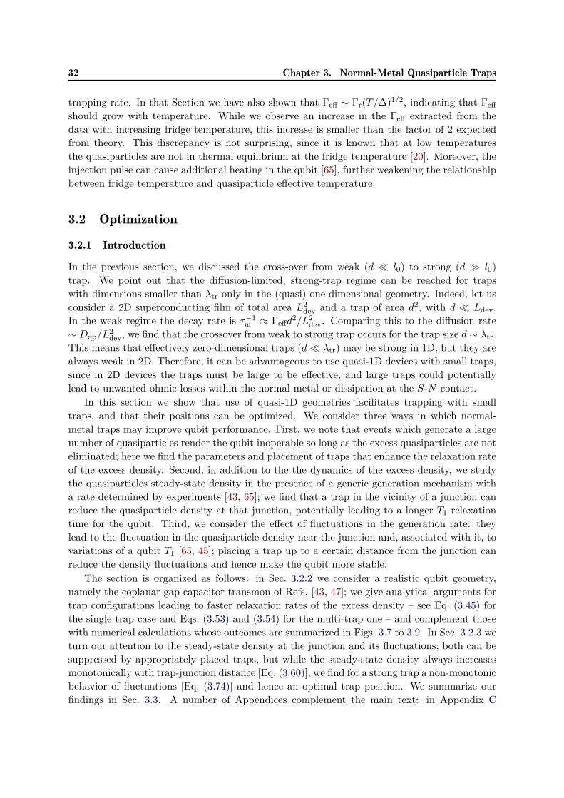
32 Chapter 3. Normal-Metal Quasiparticle Traps
trapping rate. In that Section we have also shown that Γeff ∼ Γr(T/∆)1/2, indicating that Γeffshould grow with temperature. While we observe an increase in the Γeff extracted from thedata with increasing fridge temperature, this increase is smaller than the factor of 2 expectedfrom theory. This discrepancy is not surprising, since it is known that at low temperaturesthe quasiparticles are not in thermal equilibrium at the fridge temperature [20]. Moreover, theinjection pulse can cause additional heating in the qubit [65], further weakening the relationshipbetween fridge temperature and quasiparticle effective temperature.
3.2 Optimization
3.2.1 Introduction
In the previous section, we discussed the cross-over from weak (d l0) to strong (d l0)trap. We point out that the diffusion-limited, strong-trap regime can be reached for trapswith dimensions smaller than λtr only in the (quasi) one-dimensional geometry. Indeed, let usconsider a 2D superconducting film of total area L2
dev and a trap of area d2, with d Ldev.In the weak regime the decay rate is τ−1
w ≈ Γeffd2/L2
dev. Comparing this to the diffusion rate∼ Dqp/L
2dev, we find that the crossover from weak to strong trap occurs for the trap size d ∼ λtr.
This means that effectively zero-dimensional traps (d λtr) may be strong in 1D, but they arealways weak in 2D. Therefore, it can be advantageous to use quasi-1D devices with small traps,since in 2D devices the traps must be large to be effective, and large traps could potentiallylead to unwanted ohmic losses within the normal metal or dissipation at the S-N contact.
In this section we show that use of quasi-1D geometries facilitates trapping with smalltraps, and that their positions can be optimized. We consider three ways in which normal-metal traps may improve qubit performance. First, we note that events which generate a largenumber of quasiparticles render the qubit inoperable so long as the excess quasiparticles are noteliminated; here we find the parameters and placement of traps that enhance the relaxation rateof the excess density. Second, in addition to the the dynamics of the excess density, we studythe quasiparticles steady-state density in the presence of a generic generation mechanism witha rate determined by experiments [43, 65]; we find that a trap in the vicinity of a junction canreduce the quasiparticle density at that junction, potentially leading to a longer T1 relaxationtime for the qubit. Third, we consider the effect of fluctuations in the generation rate: theylead to the fluctuation in the quasiparticle density near the junction and, associated with it, tovariations of a qubit T1 [65, 45]; placing a trap up to a certain distance from the junction canreduce the density fluctuations and hence make the qubit more stable.
The section is organized as follows: in Sec. 3.2.2 we consider a realistic qubit geometry,namely the coplanar gap capacitor transmon of Refs. [43, 47]; we give analytical arguments fortrap configurations leading to faster relaxation rates of the excess density – see Eq. (3.45) forthe single trap case and Eqs. (3.53) and (3.54) for the multi-trap one – and complement thosewith numerical calculations whose outcomes are summarized in Figs. 3.7 to 3.9. In Sec. 3.2.3 weturn our attention to the steady-state density at the junction and its fluctuations; both can besuppressed by appropriately placed traps, but while the steady-state density always increasesmonotonically with trap-junction distance [Eq. (3.60)], we find for a strong trap a non-monotonicbehavior of fluctuations [Eq. (3.74)] and hence an optimal trap position. We summarize ourfindings in Sec. 3.3. A number of Appendices complement the main text: in Appendix C

Chapter 3. Normal-Metal Quasiparticle Traps 33
we compare trapping by normal-metal traps with that due to vortices; Appendix D presentsome mathematical details for the case of a single, finite-size trap, and Appendix E addressesthe question of the experimental observability of the slowest decay rate of the excess density;Appendices F.1 and F.2 contain details about the mapping of a realistic qubit design into a 1Dwire. In Appendix G we present details about how to find the slowest decay rate having singleor multiple traps as well as details of finding the steady-state density. Finally, Appendix Hconsiders traps in the Xmon qubit geometry.
3.2.2 Enhancing the decay rate of the density
In this part we analyze how to optimally place traps of a given size, so that the slowest mode ofthe quasiparticle density decays as fast as possible. As a concrete example, we take the coplanargap capacitor transmon and study traps placed in the long wire connecting the gap capacitor tothe antenna pads, both via analytical and numerical approaches. For actual estimates, we usethe parameters measured in Refs. [47, 43], namely Γeff = 2.42 × 10⁵ Hz and Dqp = 18 cm2/s,which using Eq. (3.21) give λtr ' 86.2 µm. Since we are interested in the decay of the excessdensity, we can set g = 0; the effect of a trap on the steady-state density due to finite g is thefocus of Sec. 3.2.3. In Appendix C, we compare trapping by vortices [43] to normal-metal traps.
As we discuss at the end of Sec. 3.2.2.1, considering only the slowest mode for the opti-mization may not be sufficient when addressing the extreme case of a single, very large trap.However, as we have already pointed out, in a quasi-1D geometry short traps can be strong –that is, effective at suppressing the excess quasiparticle density. In this case the slowest modein general still suffices to characterize the long-time quasiparticle decay. The short-trap regimeis in particular important for the multiple-trap configurations considered in Sec. 3.2.2.2: theseconfigurations combine a fast decay of the quasiparticle density with low electromagnetic losses,and are thus preferable.
3.2.2.1 Optimization for a single trap
Let us consider a single trap placed in the antenna wire of length L, see Fig. 3.6 (the devicebeing symmetric, there are two traps in total). We start for simplicity with a short trap oflength d λtr and neglect the gap capacitor and antenna pads; we then show how to map thefull device to this simpler configuration and compare our estimates with numerical results.
For a short trap in a wire, the diffusion equation (3.19) can be written in the form (cf.Appendix D)
xqp = Dqp~∇2xqp − γeffδ (y − L1)xqp . (3.42)
The trap is at position y = L1 and γeff = dΓeff. Consider for simplicity the case γeff → ∞,such that quasiparticles are trapped immediately once they reach the trap. As a consequence,xqp(L1) = 0, and the density on the left and right sides of the trap decays with the ratesτ−1w = π2Dqp/4L2
1 and τ−1w = π2Dqp/4(L−L1)2, respectively. If the trap is at the center of the
wire, L1 = L/2, the density decays equally fast on both sides, and the decay rate of the slowestmode is four times faster as compared to placing the trap at the beginning or end of the wire.In other words, the central position is the optimal one for the trap to evacuate quasiparticlesas quickly as possible.

34 Chapter 3. Normal-Metal Quasiparticle Traps
At finite γeff, the left/right modes are coupled, but the coupling is small provided that thetrap is strong, d l0. The coupling lifts the mode degeneracy at L1 = L/2, but does notchange the above conclusion on the optimal position. We note, however, that if quasiparticlesare injected and detected locally (as, e.g., in [47]) one may not necessarily observe the globalslowest decay rate for strong traps; see Appendix E for more details.
In the simple example above we have shown that the optimal trap position (for which thedecay rate of the slowest mode is the fastest) is such that the diffusion times in both sides ofthe trap are equal. We can extend this finding to a more realistic qubit geometry [47] whichincludes the coplanar gap capacitor close to the Josephson junction and the antenna pad at thefar end of the wire, see Fig. 3.6. The capacitor “wings” of length Lc and the square pad with sideLpad can be accounted for by adding some effective lengths to the antenna wire. The effectivelengths Leff
c (k) and Leffpad (k) (for capacitor and pad, respectively) in general depend on the wave
vector k, see Appendices F.1 and F.2. If these effective lengths are much smaller than the wirelength L, we find that for the slow modes the dependence on k drops out: Leff
pad ≈ L2pad/W
and Leffc ≈ 2Wc
W Lc, with W and Wc the widths of of the wire and capacitor wings, respectively.These effective lengths may simply be added to the lengths to the left and right of the trap tofind the decay rates:
1τw
= π2Dqp
4(L− L1 + L2
pad/W − d/2)2 (3.43)
Figure 3.6: Top: sketch of the transmon qubit studied here, based on the experiments ofRef. [47] reported in section 3.1. Light blue/light gray: superconducting material; red/darkgray: regions of the superconductor covered by normal metal; cross: position of the Josephsonjunction. Except for the junction region, the sketch is to scale. Bottom: right half of the device,with the relevant lengths defined: a trap of length d is placed on the antenna wire (length L,width W ) at distance L1 from the gap capacitor (dimensions Lc and Wc.) The antenna pad isa square of side Lpad.

Chapter 3. Normal-Metal Quasiparticle Traps 35
for the right mode and1τw
= π2Dqp
4(L1 + 2Wc
W Lc − d/2)2 (3.44)
for the left mode; we have accounted for the finite size of the trap by subtracting the d/2 termsin the denominators, and L1 denotes the trap center. Thus, the optimal trap position is (in thestrong trap limit):
Lopt = L
2 +Leffpad − Leff
c
2 . (3.45)
The optimal position is closer to the pad (gap capacitor) if the effective length of the pad(capacitor) is larger.
We can check the validity of the above considerations for strong traps and extend ourconsideration to weaker (i.e., smaller) traps by more accurately modelling the diffusion- seeAppendix G.1.1 for details of calculations. The density in the parts not covered by the trap iswritten in the form
xqp(t, y) = e−t/τw [α cos ky + β sin ky] (3.46)
with 1/τw = Dqpk2 (except for the pad, where the density is assumed uniform), while under
the trap we havexqp(t, y) = e−t/τw [α cosh y/λ+ β sinh y/λ] . (3.47)
Imposing continuity of xqp and current conservation we find:
z2 + b2 = (L/λtr)2 , (3.48)z
b[az + tan (zξR)]
[1− h (z, ξL) tanh
(bd
L
)]−[1− az tan (zξR)]
[tanh
(bd
L
)− h (z, ξL)
]= 0, (3.49)
with z = kL, b = L/λ, a = L2pad/(LW ), and
h (z, ξL) = z
b
tan (zξL) + tan(z lL
)+ 2Wc
W tan(zLcL
)1− tan (zξL)
[tan
(z lL
)+ 2Wc
W tan(zLcL
)] . (3.50)
We also define the (normalized) length of the wire to the left (right) of the trap by
ξL = (L1 − d/2) /L , (3.51)ξR = (L− L1 − d/2) /L . (3.52)
Solving Eqs. (3.48) and (3.49) for z and b, one can find the density decay rate 1/τw = Dqpz2/L2.
For a long qubit with L λtr, the slow modes have b ≈ L/λtr 1 and z ∼ 1. We note thatthe assumption of uniform density in the pad requires 1/τw = Dqpz
2/L2 Dqp/L2pad; since for
experimentally relevant parameters we have L2pad/L
2 ∼ 10−2, the assumption is valid for slowmodes even when z & 1. In Fig. 3.7 we show a density plot of the decay rate 1/τw as a functionof the distance L1 between gap capacitor and trap center and of the normalized trap size d/l0,calculated using typical experimental parameters as detailed in the caption. For a strong trap,d l0, as discussed in Sec. 3.1.3.2 we find that the decay rate is sensitive to the trap position.

36 Chapter 3. Normal-Metal Quasiparticle Traps
Figure 3.7: Trapping rate 1/τw as a function of the trap position L1 (in units of L) andnormalized trap size d/l0 – see Fig. 3.6 for the device geometry; the device parameters are (alllengths in µm): L = 1000, l = 60, W = 12, Lc = 200, Wc = 20, Spad = L2
p = 802. We usedλtr = 86.2 µm for the trapping length, so l0 = πλ2
tr/2L ' 11.7 µm. The white areas are regionsin which the trap center cannot be pushed closer to or further away from the gap capacitor dueto the finite trap size.
The optimum position is shifted with respect to the middle of the wire (dash-dotted line inFig. 3.7), in agreement with the prediction of Eq. (3.45). Indeed, for the parameters in Fig. 3.7,we find Leff
pad = L2pad/W ≈ 533µm and Leff
c = 2WcW Lc ≈ 667µm, and the optimal position is
closer to the gap capacitor. When the trap size is d . l0, the trap position has only a minoreffect on the trapping rate. This is more clearly seen in Fig. 3.8 (bottom solid curve). Forlonger traps, we compare the decay from the numerical solution to Eqs. (3.48) and (3.49) withEqs. (3.43) and (3.44). When the trap is strong but still short compared to the wire (middlesolid), Eqs. (3.43) and (3.44) (dashed) provide a good approximation to the numerical results (infact, one can expect the numerically calculated rate to be slower than the analytical prediction,since the numerics account for the finite trapping length which allows for finite density underthe trap as well as for the bridge of length l joining the junction to the gap capacitor). For verylong traps (upper solid line) the approximation that the effective lengths are small compared tothe (uncovered part of the) wire fails, and the calculated rate is faster; this is qualitatively inagreement with the fact that as the mode wavelength increases, the effective lengths decrease,see Eqs. (F.4) and (F.7) (for the gap capacitor, this is true so long as 2Wc/W > 1).
Our focus so far has been in speeding up the decay rate of the slowest mode, without takinginto consideration the amplitude of the mode at the junction. This approach is correct for

Chapter 3. Normal-Metal Quasiparticle Traps 37
0.0 0.2 0.4 0.6 0.8 1.00
1
2
3
4
5
6
7
L1/L
1/τw(ms-1)
Figure 3.8: Solid lines: trapping rate 1/τw as a function of the trap position L1 measured inunits of L for (top to bottom) d/l0 = 40, 10, 1; other parameters are specified in the captionto Fig. 3.7 and the device geometry is shown in Fig. 3.6. The dashed lines are the estimatesprovided by Eqs. (3.43) and (3.44) for d/l0 = 40, 10.
weak traps, d . l0, since the amplitude of the mode is approximately the same on both sidesof the trap. For strong but small traps, l0 d . λtr, the amplitude on one side of the trapis algebraically suppressed by a factor of order d/l0 compared to the amplitude on the otherside (see Appendix E), while for long traps, d λtr the suppression is exponential in d/λtr (seeAppendix D). In the latter case, it would clearly be advantageous to place the trap close to thejunction: the mode with large amplitude between junction and trap would decay quickly, whilethe slow mode with large amplitude on the other side of the trap would decay slowly but itwould be exponentially suppressed at the junction. However, as we already pointed out, longtraps could be too lossy – this motivates us to further study how to obtain the fastest possibledecay using only small traps.
3.2.2.2 Multiple traps
We now generalize the considerations of the previous section to the case of multiple traps (ineach half of the qubit). For a weak trap, the effective trapping rate is proportional to the trapsize [Eq. (3.36)] but independent of position; therefore, no change in the density decay rate canbe expected by dividing a weak trap into smaller ones, since the total size is unchanged. Thestrong-trap regime is qualitatively different in this regard. Let us consider Ntr strong traps ina wire of length L; the traps separate the wire into Ntr + 1 compartments. The optimal trapplacement is obtained when the diffusion time is the same for each compartment, meaning thatthe traps have to be placed at positions Ln = (2n − 1)L/2Ntr with n = 1, . . . , Ntr, and the

38 Chapter 3. Normal-Metal Quasiparticle Traps
resulting decay rate is
τ−1w (Ntr) = N2
trDqpπ2
L2 . (3.53)
The rate increases quadratically with the number of traps, so splitting a single strong trap intosmaller pieces can highly increase the decay rate. However, when keeping the total area ofthe traps constant, there is a limitation to this improvement. Indeed, the length of each trapdecreases as d/Ntr and the “device length” of each compartment is of order L/2Ntr; using thesequantities in Eq. (3.34) we find that the traps cross over to the weak regime for
Nopttr ∼
√d
2l0; (3.54)
here l0 is defined by the right hand side of Eq. (3.34) with Ldev = L. Increasing the trap numberbeyond Nopt
tr does not further improve the decay rate, which is thus limited by Eq. (3.36). Inother words, to obtain that maximum decay rate for given total length d, at least Nopt
tr trapsshould be placed evenly spaced over the device. Such a configuration could also reduce thetrap-induced losses, since they depend on the trap position and size [75].
Let us now show in a concrete example that multiple traps can indeed increase the decayrate as predicted by Eq. (3.53). We consider again the transmon device depicted in Fig. 3.6,but we now assume that two traps are placed on the central wire, with distances L1 and L2between the gap capacitor and the traps centers. Accounting for the second trap, we generalizeEq. (3.49) to
z
b
[1− h(z, ξL) tanh
(bd1L
)]z
btan (zχ)− tanh
(bd2L
)+ g(z)
[1− z
btan (zχ) tanh
(bd2L
)]−[tanh
(bd1L
)− h(z, ξL)
]tanh
(bd2L
)tan (zχ)
+ z
b− g(z)
[tan (zχ) + z
btanh
(bd2L
)]= 0
(3.55)
where, taking L1 < L2,
ξL = (L1 − d1/2)/L (3.56)ξR = (L− L2 − d2/2)/L (3.57)χ = (L2 − d2/2− L1 − d1/2)/L , (3.58)
the function h(z, ξL) is defined in Eq. (3.50), and
g(z, ξR) = z
b
az + tan z(1− L1+χ+d2/2L )
1− az tan z(1− L1+χ+d2/2L )
. (3.59)
We consider for simplicity the case of equal traps, d1 = d2 ≡ d/2 with d = 20l0 ' 233µm thetotal length of the normal metal. We show in Fig. 3.9 the decay rate as function of L1 and L2for the same parameters as in Fig. 3.7. We find that the decay rate is highest when placing thetraps far away from each other, one trap touching the gap capacitor and the other begin close

Chapter 3. Normal-Metal Quasiparticle Traps 39
(a)
(b)
Figure 3.9: (a) Device with two traps (dark red) in each half of the qubit; distances L1 and L2are measured from the gap capacitor to the center of each trap, cf. Fig. 3.6. (b) Trapping rate1/τw as function L1 and L2; here the two traps are identical, d1 = d2 = 10l0, which makes theplot symmetric under the exchange L1 ↔ L2. The parameters used are specified in the captionto Fig. 3.7. Similar to that figure, the white areas correspond to forbidden regions due to thefinite traps’ sizes . A comparison with Fig. 3.7 reveals that splitting a trap with length d = 20l0into two identical ones can boost the trapping rate up to a factor larger than 3.
to the pad. We find that the decay rate of the slowest mode is highest when placing the trapsfar away from each other, one trap touching the gap capacitor and the other begin close to thepad. This is in qualitative agreement with expectations: consider again the gap capacitor andthe pad as extra lengths added to the left and right of the central wire, respectively; this leadsto a wire of effective total length Ltot = Leff
c +L+Leffpad ' 2200µm. In such a wire the optimal
positions would be L1 = Ltot/4 ' 550µm and L2 = 3Ltot/4 ' 1650µm. The value of L1 wouldindicate an optimal position inside the gap capacitor, but since we allow for the traps to move in

40 Chapter 3. Normal-Metal Quasiparticle Traps
the central wire only, this optimal placement is not possible. The value of L2 corresponds to aposition slightly away from the pad, in agreement with the results in Fig. 3.9. Finally, going fromthe optimally-placed single trap to the optimal two-trap configuration, the decay rate increasesby a factor of ∼ 3.4. This factor does not reach the theoretical maximum of 4 predicted byEq. (3.53); the discrepancy can be attributed both to the non-optimal placement of the firsttrap mentioned above as well as to finite-size effects, as in the single trap case. However, thecalculated improvement confirms that the decay rate can be significantly increased by optimizingthe trap number and position.
It is instructive to compare our results for the two-trap case with the fast decay of themode to the left of the single trap; using Eq. (3.44), we estimate the decay rate of this modeto be 1/τw ' 14.7ms−1, slightly slower than the maximum rate shown in Fig. 3.9. In bothcases, we do not allow the trap to enter the gap capacitor; this constraint could be importantin limiting trap-related losses, as the gap capacitor is the region with the highest electric field.Using two traps we place only half the total normal material near the high-field region, whileobtaining a slightly faster decay than with a single, large trap. For the considered example,further increase in the decay rate could be obtained by further splitting the traps. Indeed, amore accurate estimate for the length l0 can be obtained by using Ldev = Ltot−d ' 1967µm inEq. (3.34), giving l0 ≈ 5.9µm. Then the “optimal” trap number would be Nopt
tr '√d/2l0 ∼ 4,
requiring one trap to be placed on the pad, two on the antenna wire, and one on the gapcapacitor (this placement is calculated using the “effective wire” length of the gap capacitor,so that in practice one should symmetrically place one trap on each of the two “wings” of gapcapacitor). As mentioned above, placement on the gap capacitor could be detrimental, but withthe optimal trap number only one quarter of the normal metal would be in the gap capacitor andthe resulting losses would therefore be smaller than those due to a single large trap on the gapcapacitor. Therefore, it is potentially beneficial to have multiple smaller traps in comparisonwith a single large trap. Such considerations are also dependent on the device design, and inAppendix H we briefly consider a different geometry for the qubit, the Xmon of Ref. [17]; thecentral X-shaped part of the device is small, and unfortunately this implies that no large gainin the decay rate can be obtained using multiple traps, so alternative approaches are desirablein this case. In the next section we turn our attention to the effect of traps on the steady-statedensity.
3.2.3 Suppression of steady-state density and its fluctuations
In the preceding subsection we have dealt with the question of how fast quasiparticles reachtheir steady state if there is a deviation from said steady-state density. In this part we pointout that traps also affect the shape of the steady-state density. In particular, our aims are tominimize the steady-state density at the junction, which directly affects the T1 time of qubits,as well as to stabilize the density value against fluctuations in their generation rate which leadto temporal variations in the qubit lifetime. In our model, the steady-state density is nonzerodue to a finite generation rate g in Eq. (3.19). As argued in Sec. 3.1.3.2, in the presence of aweak trap the quasiparticle density is uniform, and in the steady-state takes the value xsqp = gτwwith τw of Eq. (3.36). As we now show, going beyond the weak limit the geometry affects thespatial profile of the density.
For a concrete example, we consider the same geometry as in Sec. 3.2.2.1 – that is, a single

Chapter 3. Normal-Metal Quasiparticle Traps 41
trap on the wire connecting gap capacitor and pad, see Fig. 3.6. The solution for the profileof the steady-state density in each 1D segment outside the trap is given by parabolas of thegeneral form xsqp = −y2g/2Dqp + αy + β, while under the trap we have xsqp = α cosh(y/λtr) +β sinh(y/λtr) + g/Γeff. The parameters α, β in each segment, as well as α, β are found byimposing appropriate boundary conditions (i.e., continuity and current conservation). We finallyarrive at the following expression for the steady-state density xJqp at the junction:
xJqp = g
Γeff
1 + 1
sinh(d/λtr)
[ARWλtr
+ cosh(d/λtr)ALWλtr
]+ g
Dqp
[(L1 + l − d/2)2
2 + Ac(L1 − d/2)W
],
(3.60)
where AR = W [L− L1 − d/2] + L2pad and AL = W [L1 + l − d/2] + Ac are the uncovered areas
to the right and left of the trap, respectively, and Ac = 2WcLc is the gap capacitor area.In the small trap limit, d λtr, we can rewrite Eq. (3.60) in the form
xJqp ' g (τw + tD) (3.61)
with τw defined in Eq. (3.36), while tD = [(L1 + l− d/2)2/2 +Ac(L1− d/2)/W ]/Dqp representsthe diffusion time between junction and trap (with the second term in square brackets takinginto account the presence of the gap capacitor). Similar to the discussion in Sec. 3.1.3.2,we can distinguish between an effectively weak (τw tD) and strong trap (τw tD), withthe trap becoming strong as its length d increases above the position-dependent length scalel1 ∼ λ2
tr/√DqptD. Note that l1 decreases with the distance L1 between gap capacitor and trap
and is always larger than l0 of Eq. (3.34); therefore a trap that is weak in the sense of d beingsmaller than l0 is weak at any position L1, and the value of xJqp is only weakly dependent on thetrap placement. On the other hand, a strong trap with d > l0 effectively becomes weak, as L1decreases, when τw = tD. At positions L1 smaller than that given by this condition, xJqp againbecomes weakly dependent on trap placement. In other words, the condition determines themaximal distance at which the largest (up to numerical factor) suppression of xJqp is achievedfor a given trap size d.
For a long trap d λtr, we can still use Eq. (3.61) after the identification
τw →1
Γeff
(1 + AL
Wλtr
). (3.62)
With this substitution and for typical experimental parameters, we find again that the first termin Eq. (3.61) dominates when the trap is close to the junction (despite being smaller than thecorresponding term for a short junction), while the second one takes over as L1 increases. Moregenerally, it should be noted that in any regime xJqp is a monotonically increasing function of L1:as one could expect, the closer the trap is to the junction, the more it suppresses the quasiparticledensity near the latter. This behavior is evident in Fig. 3.10: the plot clearly shows that thedensity is suppressed by placing the trap near to the gap capacitor, and that long traps (d & λtr)are more effective. Values as low as xqp ∼ 10−8 are predicted; for comparison, we note thatin devices with the geometry considered here but without traps, we estimate xqp ∼ 10−6 [43].On the other hand, for transmons with larger pads (so that there are always vortices that actas traps) we find xqp ∼ 10−7 [6, 43]. Further suppression of the density could be achieved by

42 Chapter 3. Normal-Metal Quasiparticle Traps
Figure 3.10: Quasiparticle density at the junction as a function of trap location L1 (in unitsof L) and its normalized size d/λtr, calculated using g = 10−4 Hz [43, 65]; the normalizationof the size d differs from that of Fig. 3.7, but the parameters used for the device are the samespecified there.
placing traps in the gap capacitor, since this would effectively reduce the uncovered area AL[cf. Eq. (3.62)] between trap and junction.
Based on the above consideration, we do not expect that adding a second trap far fromthe junction significantly affects the steady-state density xJqp (we have confirmed this by directcalculation). Therefore, the results of the last two sections suggest that having two traps, oneclose to the junction and the other close to the pad can both greatly reduce the steady-statedensity at the junction and enhance the decay rate of the excess density. Next, we show thattraps can also contribute to the temporal stability of the qubit.
3.2.3.1 Fluctuations in the generation rate
As discussed previously, the density at the junction and hence the qubit relaxation rate areproportional to the generation rate g. Therefore, temporal variations in g can cause changes inthe measured T1 over time. Here we explore how traps can suppress these changes. For thispurpose, we include Gaussian fluctuations of g in Eq. (3.19) by replacing g → g+ δg (y, t), with
〈δg (y, t)〉 = 0 , (3.63)⟨δg (y, t) δg
(y′, t′
)⟩= γgδ
(y − y′
) 12τm
e−|t−t′|τm . (3.64)
The parameter γg characterizes the fluctuation amplitude and has the same units as γeff ofEq. (3.42), while 〈. . .〉 averages over all realizations of δg. We assume that fluctuations are

Chapter 3. Normal-Metal Quasiparticle Traps 43
spatially uncorrelated, but allow for temporal correlations with a finite memory time τm – wewill return to this point in what follows. Note that under these assumptions the average density〈xqp(y)〉 is in general a function of the spatial coordinate due to the presence of traps, but notof time.
Assuming the junction to be at position y = 0, to provide a measure for the fluctuations inthe density at that point we consider the quantity
∆x2qp(t, t′)≡⟨xqp (0, t)xqp
(0, t′
)⟩− 〈xqp (0)〉2 . (3.65)
This quantity can be expressed in terms of the eigenvalues µk < 0 and eigenfunctions nk(y) ofEq. (3.19) (cf. Ref. [47] and Appendix D). Indeed, the quasiparticle density with the fluctuationterm is
xqp (y, t) =−∑k
1µknk (y) gk
+∑k
∫ t
−∞dt1e
µk(t−t1)nk (y) δgk (t1) ,(3.66)
withδgk (t1) =
∫ L
0
dy′
Lnk(y′)δg(y′, t1
), (3.67)
and the similar definition for gk. Substituting this expression into the definition Eq. (3.65) andaveraging over the fluctuations, we find
∆x2qp(t, t′)
= γg2L
1τm
∑k
∫ t
−∞dt1
∫ t′
−∞dt2 e
µk(t−t1)
×eµk(t′−t2)e−|t1−t2|τm n2
k (0) .
(3.68)
The time integrals are conveniently computed by first shifting the times t1 and t2 by t andt′, respectively, and then changing variables in the two-dimensional integral into a mean timet1 + t2 and time difference t1 − t2. After integration, we obtain
∆x2qp(t− t′
)= γg
2L∑k
τme−|t−t
′|τm + 1
µkeµk|t−t
′|
τ2mµ
2k − 1
n2k (0) , (3.69)
which depends only on time difference.Equation (3.69) shows that even in the absence of time correlations for the fluctuations in
the generation rate, τm = 0, the fluctuation in the density are correlated due to diffusion. In thiscase, the longest decay time is that of the slowest mode, 1/µ0, and is typically of the order ofmilliseconds [47]. This time is shorter than the time it takes to measure a qubit relaxation curveand hence estimate the quasiparticle density. Therefore, only the regime in which τm is muchlonger than 1/µ0 could have observable consequences. Moreover, there is experimental evidencefor slow fluctuations in the number of quasiparticles in qubits, obtained by monitoring thequantum jumps between states of a fluxonium, Ref. [65], and by repeated measurements, overseveral hours, of the relaxation time in a capacitively shunted flux qubit, Ref. [45]. Therefore,

44 Chapter 3. Normal-Metal Quasiparticle Traps
in the reminder of this Section we focus only on the regime of long memory – that is, slowfluctuation in the generation rate. In the limit τm 1/µ0, Eq. (3.69) simplifies to
∆x2qp(t− t′
)' γg
2Lτme−|t−t′|τm
∑k
1µ2k
n2k (0) . (3.70)
We now want to establish that a trap can indeed reduce the fluctuations. To this end, weconsider the simple case of the junction in a quasi-1D wire extending for length L from thejunction and with a trap at distance L1 from the junction. Initially, we take the trap to besmall (length d λtr), and we distinguish between weak and strong trap, see Eq. (3.34). Fora weak trap, d l0, the slow modes are only weakly dependent on the spatial coordinate.Moreover, for the slowest mode the decay rate is [cf. Eq. (3.36)]
µ0 ≈ −Γeffd
L, (3.71)
while the higher modes are much faster, since µn>0 . −Dqp/L2, and thus |µn>0| |µ0|. Using
n0(0) ≈ 1 and neglecting the small contributions from the higher modes, from Eq. (3.70) wefind
∆x2qp(t− t′
)≈ γg
2Lτme−|t−t′|τm
(L
Γeffd
)2. (3.72)
This expression shows that a stronger/longer trap more effectively suppresses fluctuation, ascould be expected.
In the case of a strong trap (d l0), the eigenmodes can be split in two sets: thereare left and right modes, which are strongly suppressed to the right and to the left of thetrap, respectively (here we assume that the trap position is sufficiently far from the centralposition, see Appendix E). The left modes, with large amplitude between junction and trap,give small contributions to the density fluctuations when the trap is close to the junction andtheir contributions grow with junction-trap distance. The right modes, while being suppressedto the left of the trap, have opposite behavior with distance, so they can dominate when the trapis sufficiently close to the junction. Then we generically expect a non-monotonic dependence ofthe density fluctuations on trap-junction distance from the competition between modes to theleft and right of the trap.
Indeed, let us consider the decay rates for left and right modes, which we denote with µn,L1
and µn,L−L1 , respectively, where we define
µn,` ' −Dqp
(π
2`
)2(2n+ 1)2 , n = 0, 1, . . . (3.73)
Keeping in Eq. (3.70) only the slowest mode for each set, since the higher modes with n > 0gives a smaller contribution to the sum, we find
∆x2qp(t− t′
)≈ γgLτm
e−|t−t′|τm
1µ2
0,L
×[(
L1L
)3+(l0d
)2 L− L1L
],
(3.74)
where we used n2k,L1
(0) ' 2L/L1 and n2k,L−L1
(0) ' 2(l0/d)2[L/(L− L1)]3 (here we also assumed L1, L − L1). The first term in square brackets originates from the lowest mode confined

Chapter 3. Normal-Metal Quasiparticle Traps 45
between junction and trap, while the second term, due to the lowest mode located on theother side of the trap, is suppressed by the small factor (l0/d)2. As a function of the trapposition L1, in agreement with the above considerations we find that ∆x2
qp has a minimumat L1 = Ll0/d
√3, where the terms in square brackets take the approximate value (l0/d)2 and
Eq. (3.74) takes the same form of Eq. (3.72). In fact, those terms rise significantly above thisvalue only for L1 > Lf ≡ L(l0/d)2/3, indicating that for a strong trap a large suppression offluctuations can be achieved if the trap is not placed far beyond Lf . We note that this conditionis more stringent than the one discussed after Eq. (3.61), τw = tD, which for the simple wireconsidered here gives a maximum distance ∼ 2L
√l0/πd; in other words, maximum suppression
of fluctuations ensures maximum suppression of the steady-state density.The above considerations for a strong but short trap can be generalized to longer traps
(d & λtr, with d L) by substituting l0/d → λtr/L sinh(d/λtr), see Appendix D. In bothregimes (strong but short, and long trap), increasing the trap length suppresses the fluctuationsat the junction, but shrinks the region over which maximum suppression can be achieved,since Lf becomes smaller. This region is however always small compared to the wire length,Lf L. Together with the monotonic dependence of the average quasiparticle density ondistance obtained in the first part of this section, our results show that placing a trap close tothe junction is effective in suppressing both the average density and its fluctuations, potentiallymaking the qubit longer lived and more stable.
3.3 Summary and Conclusions
In section 3.1 we developed a basic model enabling us to predict the effect of a normal-metaltrap on the dynamics of the nonequilibrium quasiparticles population in a superconductingqubit. The model accounts for the tunneling between the superconductor and the trap, as wellas for the electron energy relaxation in the trap, see Eq. (3.18). The surprising finding is thatthe effective trapping rate Γeff is sensitive to the energy of the quasiparticles and is constrainedby their backflow from the normal-metal trap on time scales shorter than the electron energyrelaxation rate. Furthermore, we find the dependence of the time needed to evacuate the injectedquasiparticles on the trap size. The evacuation time saturates at the lowest, diffusion-limitedvalue upon extending the trap above a certain characteristic length l0; the dependence of l0 onthe parameters of the trap and qubit is given in Eq. (3.34).
The experimental data (obtained by our collaborators in Yale University) reported in Sec. 3.1.4validate the theoretical model. The relaxation rate 1/T1 of a transmon qubit is proportional tothe quasiparticle density in the vicinity of the Josephson junction, making it possible to measurethe dynamics of the quasiparticle population. We find that the population decay rate increaseswith the length of the normal-metal traps, in agreement with the predicted cross-over from weakto strong trapping, see Fig. 3.5. For small traps we can estimate the effective trapping rate Γeff:both its order-of-magnitude and its increase with temperature indicate indeed a limitation dueto the backflow of quasiparticles.
Utilizing traps is a viable strategy of mitigating the detrimental effect of quasiparticles on thequbits T1 time. Further improvement of normal-metal traps may benefit from finding ways toshorten the electron energy relaxation time in them. Based on the experiments of Refs. [58, 59],using a different pure metal (e.g., silver or gold) for the trap is unlikely to result in substantiallyshorter relaxation time; metals hosting magnetic impurities might be helpful in this regard, but

46 Chapter 3. Normal-Metal Quasiparticle Traps
such impurities could harm the qubit by opening other relaxation channels.In section 3.2 we studied the effects of size and position of normal-metal quasiparticle traps in
superconducting qubits with large aspect ratio, so that quasiparticle diffusion can be consideredone-dimensional. We focus on such a design because, as we argued at the begening of thatsection, in a two-dimensional setting traps must be large compared to the trapping length λtr ofEq. (3.21) to be strong, while in quasi-1D it is sufficient for the trap length d to be longer thanthe characteristic scale l0 [Eq. (3.34)] which accounts for diffusion, trapping rate, and device size– this characteristic scale is generally shorter than λtr for long devices (Ldev > λtr). A trap caninfluence the qubit in three ways: first, it suppresses the steady-state quasiparticle density at thejunction; then the qubit’s T1 time can be increased, since this time is inversely proportional tothe density. Second, a trap can speed up the decay of the excess quasiparticles and, third, it candecrease fluctuations around the steady-state density; these effects can render the qubit morestable in time – in fact, there is experimental evidence (Refs. [45] and [65]) that fluctuationsin the number of quasiparticles are responsible for at least part of the temporal variations inT1. Not surprisingly, a long trap (d & λtr) placed close to the junction is effective in all threeaspects: fast decay of excess quasiparticles, suppression of the steady-state quasiparticle density(see Fig. 3.10), and suppression of density fluctuations at the junction. However, large trapscould be a source of unwanted dissipation; therefore, we analyze in more detail the effects ofshorter traps.
If a trap is weak, d . l0, its position has little influence on the ability to suppress thequasiparticle density and its fluctuations, as well as on the decay rate of excess quasiparticles.Interestingly, for a strong but short trap, l0 . d . λtr, we find the position of the trap can beoptimized in several ways. First, there is an optimal position that makes the decay of excessquasiparticles as fast as possible, see Figs. 3.7 and 3.8 in Sec. 3.2.2.1; however, a better choiceis in general to divide a strong trap into smaller traps of length ∼ l0 and distribute thosearound the device, see Sec. 3.2.2.2. For suppression of density fluctuations, we find that there isan optimal trap position, see Sec. 3.2.3.1; more importantly, we find that there is a maximumdistance Lf from the junction up to which the suppression of fluctuations is effective. Moreover,the distance up to which, for a given trap size, large suppression of the steady-state densityis achieved (Sec. 3.2.3) is longer than Lf , so that suppressing fluctuations also suppresses thesteady-state density. Therefore, by correctly placing multiple traps in the device in such a waythat one is sufficiently close to the junction, all three beneficial effects of traps can be optimized.
The optimization of trap size, number, and placement is the only readily accessible way toimprove the trap efficacy, since the effective trapping rate is limited by the energy relaxation ratein the normal metal [47], a material parameter that cannot be easily modified. We stress herethat these considerations are valid for normal islands in tunnel contact with the superconductor– traps formed by gap engineering (e.g., by placing a lower-gap superconductor in good contactwith the qubit) could behave differently and deserve further consideration.

Chapter 4
Quasiclassical Theory ofSuperconductivity
In the preceding chapter our analysis was based on the hard-gap assumption. This is justifiedprovided a high resistance at the trap-qubit contact interface which results in a low transmissioncoefficient. From now on, we aim to relax this assumption and study how this affects thequbit relaxation. In this chapter, we follow notation of references [79] and [80] and reviewhow Green’s functions are used in the context of superconductivity. We explain quasiclassicaltheory of superconductivity that simplifies the equations governing the superconducting Green’sfunctions and derive the Eilenberger equation. We then show steps in order to further simplythe formalism in the limit of dirty superconductors and derive the Usadel equation for a non-uniform normal-superconducting hybrid. This equation forms our starting point in chapter 5where we study proximity-induced modifications in the superconducting properties that comealong as side effects of normal-metal quasiparticle traps for superconducting qubits.
4.1 Gor’kov EquationsLet us start by introducing time-ordered single-particle and anomalous Green’s functions thatare defined respectively as,
GT (1, 2) = −i〈Tψ↑(r1, t1)ψ†↑(r2, t2)〉, (4.1)
FT (1, 2) = −i〈Tψ†↓(r1, t1)ψ†↑(r2, t2)〉. (4.2)
where ψ†σ(r, t) (ψσ(r, t)) creates (annihilates) one electron excitation with spin σ at position rand at time t. The time-order operator T is defined such that,
TA(t1)B(t2) = Θ(t1 − t2)A(t1)B(t2)−Θ(t2 − t1)B(t2)A(t1) (4.3)
and the step function is defined
Θ(t1 − t2) =
1, t1 > t2 ,
1/2, t1 = t2 ,
0, t1 < t2 .
(4.4)
At this point, it is convenient to write the mean-field BCS Hamiltonian, Eq. (2.4), in the firstquantized notation,
HMFBCS =
∑σ=↑,↓
∫drψ†σ(r)h(r)ψσ(r)−
∫dr(∆∗(r)ψ↑(r)ψ↓(r) + ∆(r)ψ†↓(r)ψ
†↑(r)). (4.5)

48 Chapter 4. Quasiclassical Theory of Superconductivity
where
h(r) = − 12m(∇r − ieA(r))2 + eφ(r)− µ, (4.6)
for which, for generality, we assumed presence of an electromagnetic field. We can then find theequation of motion for the electron field operators,
idψ↑(r, t)
dt= h(r)ψ↑(r, t) + ∆(r)ψ†↓(r, t), (4.7)
−idψ†↓(r, t)
dt= h∗(r)ψ†↓(r, t)−∆∗(r)ψ↑(r, t). (4.8)
Having found these, it is straightforward to calculate the equation of motion for the definedGreen’s functions that are known as Gor’kov equations,
[i ∂∂t1− h(r1)]GT (1, 2) + ∆(r1)FT (1, 2) = δ(t1 − t2)δ(x1 − x2), (4.9a)
[−i ∂∂t1− h∗(r1)]FT (1, 2) + ∆∗(r1)GT (1, 2) = 0. (4.9b)
In order to facilitate the description of particle-hole coherence in superconductors, we formulateour notation in Nambu space. We introduce the Nambu spinor and its conjugate as,
Ψ(r, t) =[ψ↑(r, t)ψ†↓(r, t)
],Ψ†(r, t) =
[ψ†↑(r, t) ψ↓(r, t)
], (4.10)
and define their multiplication as
Ψ(r1, t1)Ψ†(r2, t2) =[ψ↑(r1, t1)ψ†↑(r2, t2) ψ↑(r1, t1)ψ↓(r2, t2)ψ†↓(r1, t1)ψ†↑(r2, t2) ψ†↓(r1, t1)ψ↓(r2, t2)
], (4.11)
and
Ψ†(r1, t1)Ψ(r2, t2) =[ψ†↑(r1, t1)ψ↑(r2, t2) ψ↓(r1, t1)ψ↑(r2, t2)ψ†↑(r1, t1)ψ†↓(r2, t2) ψ↓(r1, t1)ψ†↓(r2, t2)
]. (4.12)
The Nambu spinors therefore satisfy the fermionic anti-communication rules,
Ψ(r1, t1),Ψ†(r2, t2) = δ(t1 − t2)δ(x1 − x2)τ0, (4.13a)Ψ(r1, t1),Ψ(r2, t2) = 0, (4.13b)Ψ†(r1, t1),Ψ†(r2, t2) = 0, (4.13c)
while the τ matrices are identical in form to Pauli matrices,
τ0 =[1 00 1
], τ1 =
[0 11 0
], τ2 =
[0 −ii 0
], τ3 =
[1 00 −1
]. (4.14)
The BSC Hamiltonian using the Nambu spinors then becomes,
HMFBCS =
∫drΨ†(r)HBCSΨ(r) . (4.15)

Chapter 4. Quasiclassical Theory of Superconductivity 49
for which,
HBCS =[h(r) ∆(r)
∆∗(r) −h∗(r)
]. (4.16)
The equation of motion for the Nambu spinor therefore reads,
i∂
∂tΨ(r, t) = HBCSΨ(r, t). (4.17)
We now define the time-ordered Green’s function in Nambu space as,
GT (1, 2) = −iτ3〈TΨ(r1, t1)Ψ†(r2, t2)〉
= −iτ3[〈Tψ↑(r1, t1)ψ†↑(r2, t2)〉 〈Tψ↑(r1, t1)ψ↓(r2, t2)〉〈Tψ†↓(r1, t1)ψ†↑(r2, t2)〉 〈Tψ†↓(r1, t1)ψ↓(r2, t2)〉
]
= τ3[GT (1, 2) F †T (1, 2)FT (1, 2) −G†T (2, 1)
], (4.18)
where the final equality is written in accordance with definitions given by Eqs. (4.1)-(4.2). Notethat as we have not considered spin-dependent interactions in the Hamiltonian, spin labeling isnot important that has enabled us to write 〈T (ψ†↓(r1, t1)ψ↓(r2, t2))〉 = −〈T (ψ↑(r2, t2)ψ†↑(r1, t1))〉 =−G†(2, 1).
Eq. (4.17) makes it easy to calculate the equation of motion for the defined Green’s functionfor which we find,
i∂
∂t1GT (1, 2) = ∂
∂t1τ3θ(t1 − t2)Ψ(r1, t1)Ψ†(r2, t2)− θ(t2 − t1)Ψ†(r2, t2)Ψ(r1, t1)
= τ3
δ(t1 − t2)Ψ(r1, t1),Ψ†(r2, t2)+ 〈T ( ∂
∂t1Ψ(r1, t1)Ψ†(r2, t2))〉
= τ3δ(t1 − t2)δ(r1 − r2) + HBCSGT (1, 2)
= τ3δ(t1 − t2)δ(r1 − r2) +τ3[h(r1) 0
0 h∗(r1)
]+[
0 ∆(r1)∆∗(r1) 0
]GT (1, 2).
(4.19)
We multiply both side by τ3 and find,
[G−101 + ∆BCS]GT (1, 2) = δ(t1 − t2)δ(r1 − r2), (4.20)
where,
G−101 = i
∂
∂t1τ3 + 1
2m(∇r1 − iτ3eA(r1))2 − eφ(r1) + µ, (4.21)
is the inverse free Green’s function in the Nambu space and,
∆BCS =[
0 ∆(r)−∆∗(r) 0
], (4.22)
represents the BSC-self-energy due to pairing interaction. Gor’kov was the first who showedthat the phenomenological Ginzburg-Landau model can be derived from the Gor’kov equationif temperature is close to superconducting critical temperature [81]. We note that apart fromthe BCS limit, one has to consider other self-energy terms that originate, for example, fromelectron impurity scattering. In the next section we derive left-right subtracted Dyson equationthat paves our way in formulating quasiclassical theory of superconductivity.

50 Chapter 4. Quasiclassical Theory of Superconductivity
Figure 4.1: The time loop leads to four Green’s function depending on the time variables t1 andt2 belong to which part of the contour.
4.2 Dyson Equation in Keldysh-Nambu SpaceIn formulating the perturbation theory to account for self-energy terms in the Green’s functions,one can expand the S matrix over a time loop consisting an outgoing part from (−∞, t0) anda return part from (t0,−∞). This is known as Keldysh time-loop contour, and is particularlyuseful for dealing with non-equilibrium situations where the state of the system is assumed tobe known only at time t = −∞. As depicted schematically in figure 4.1, such a time loop resultsin four types of Green’s function depending on the time variables that enter into the Green’sfunction. When both time variables belong to the outgoing part of the time loop as depictedin panel (a), we define the time-ordered Green’s function that, for superconducting systems inNambu space, is given by Eq. (4.18). If both time variables belong to the return part of the timeloop as shown by panel (b), we define the anti-time-ordered superconducting Greens’ functionas
GT (1, 2) = −iτ3〈TΨ(r1, t1)Ψ†(r2, t2)〉, (4.23)
for which the anti-time-ordered operator is defined such that,
TA(t1)B(t2) = Θ(t1 − t2)B(t2)A(t1)−Θ(t2 − t1)A(t1)B(t2). (4.24)
Finally, when the time variables are on different legs of the time loop, according to panels (c)and (d) of Fig. (4.1), we define the so-called greater and lesser Green’s functions as,
G>(1, 2) = −iτ3〈Ψ(r1, t1)Ψ†(r2, t2)〉, (4.25)G<(1, 2) = iτ3〈Ψ†(r2, t2)Ψ(r1, t1)〉. (4.26)
We now collect these four Green’s functions into a single matrix in Keldysh-Nambu space,
qG(1, 2) =[GT (1, 2) G<(1, 2)G>(1, 2) GT (1, 2)
], (4.27)

Chapter 4. Quasiclassical Theory of Superconductivity 51
where each element is a 2× 2 matrix in Nambu space.We note that, given the definitions of the so defined Green’s functions, the following identity
holds
GT + GT = G< + G>. (4.28)
Therefore, not all components of Eq. (4.27) are independent. Indeed, it is possible to removepart of the redundancy; we first rotate the Green’s function in Keldysh space by qG → τ3 qG
followed by qG → L qGL† while L = 1√2(τ0 − iτ2). These transformations lead to the Green’s
function of the form,
qG(1, 2) = 12
[GT − G< + G> − GT GT + G< + G> + GTGT − G< − G> + GT GT − G> + G< − GT
]. (4.29)
We now define the retarded, advanced and Keldysh Green’s functions as,
GR = GT − G< = G> − GT , (4.30)GA = GT − G> = G< − GT , (4.31)GK = GT + G< = G> + GT , (4.32)
We thus arrive to the triagonal representation of the Green’s function in Keldysh-Nambu space,
qG(1, 2) =[GR(1, 2) GK(1, 2)
0 GA(1, 2)
], (4.33)
which satisfies the Dyson equation,
qG(1, 2) = qG0(1, 2) +∫dX4
∫dX3 qG0(1, 4)qΣ(4, 3) qG(3, 2), (4.34)
or equivalently
qG(1, 2) = qG0(1, 2) +∫dX4
∫dX3 qG(1, 4)qΣ(4, 3) qG0(3, 2). (4.35)
Here, Xn = (rn, tn) so that the integration is over both time and space and qG0 is the Green’sfunction for free particles. The self-energy matrix qΣ contains the term originating from pairpotential as well as other terms originating, for example, from electron impurity scattering,
qΣ(1, 2) = −q∆BCS + qΣimp = −[∆BCS 0
0 ∆BCS
]+[ΣR(1, 2) ΣK(1, 2)
0 ΣA(1, 2)
], (4.36)
where ∆BCS is given by Eq. (4.22). Note that the results of the integrals in Eqs. (4.34)-(4.35)are functions of the times and coordinates labeled by 1 and 2. For brevity, we write theseequations as
qG(1, 2) = qG0(1, 2) +(
qG0 ⊗ qΣ⊗ qG)
(1, 2), (4.37a)
qG(1, 2) = qG0(1, 2) +(
qG⊗ qΣ⊗ qG0)
(1, 2), (4.37b)

52 Chapter 4. Quasiclassical Theory of Superconductivity
where ⊗ indicates matrix multiplication together with integration over time and space, and theinverse free Green’s function in Keldysh space reads,
qG−101 = i
∂
∂t1qτ3 + 1
2m(∇r1 − iqτ3eA(r1))2 − eφ(r1) + µ, (4.38)
for which
qτ3 =[τ3 00 τ3
]. (4.39)
We define qG−102 similar to qG−1
01 with the difference that the derivatives in this case are withrespect to the time and coordinate labeled by 2. We finally take,
qG−10 (1, 2) = qG−1
01 δ(1− 2) = qG−102 δ(1− 2). (4.40)
We now operate Eqs. (4.34) by qG−10 from right and integrate over time and coordinate labeled
by 1. Similarly, we operate Eqs. (4.35) by qG−10 from left and integrate over time and coordinate
labeled by 2, and then subtract the two obtained equations to find the left-right subtractedDyson equation, (
qG−10 ⊗ qG− qG⊗ qG−1
0
)(1, 2) =
(qΣ⊗ qG− qG⊗ qΣ
)(1, 2). (4.41)
The reason for this subtraction become clear in the next section where we adopt the quasiclassi-cal approximation to the left-right subtracted Dyson equation in order to drive the Eilenbergerequation.
4.3 Eilenberger EquationsThe Gor’kov equation is in principle enough to study superconductivity. In practice, however,solving the Gor’kov equation is difficult specially for situations where superconducting order pa-rameter is varying in space at temperatures far below the critical temperature Tc [83]. To finda simpler equation, we note that the Gor’kov equation contains information on the length scaleof Fermi wavelength k−1
F . This is in fact much smaller than the relevant length scales for manyphysical phenomena including proximity effect in normal-superconducting hybrids where therelevant length scale is given by the superconducting coherence length, ξ k−1
F [83, 84, 85, 90].Equivalently, the superconducting order parameter in conventional superconductors is muchsmaller than the Fermi energy, ∆/εF 1. This indicates that the magnitude of momentumin Green’s functions, and consequently in self energies that are functional of Green’s functions,is close to the Fermi momentum. In quasiclassical theory of superconductivity, one uses thispeaked structure and integrates out the momentum degree of freedom. The resulting quasiclas-sical Green’s function are then used to calculate physical quantities of interest. Formulatingthis approach was started with a seminal work done by Andreev where he employed a WKBapproximation to the Bogoliubov-de Gennes equation in order to eliminate all short wavelengthoscillations [82]. The complete quasiclassical equations for superconducting systems in thermalequilibrium were formulated by Eilenberger [85] and also independently by Larkin and Ovchin-nikov [86]. The generalization to non-equilibrium systems was done by Eliashberg [87] andLarkin and Ovchinnikov [88, 89].

Chapter 4. Quasiclassical Theory of Superconductivity 53
The starting point in quasiclassical formalism is to use the mixed or Wigner representation;in the Green’s functions, we perform a transformation to center of mass and relative coordinatesdefined by,
R = 12(r1 + r2), T = 1
2(t1 + t2), (4.42a)
r = r2 − r1, t = t2 − t1, (4.42b)
and then take a Fourier transform with respect to fast oscillating variables r and t,
qG(R, T, r, t) =∫dεe−iεt
∫dpeip.r qG(R, T, p, ε) . (4.43)
We note that the variations with respect to the center-of-mass variables are due to lack oftranslational invariance that is controlled by, for example, an applied external field or a non-uniform space.
In the quasiclassical formalism, the Green’s function is replaced by,
qG(R, p, T, ε)→ δ(ξp)g(R, p, T, ε), (4.44)
while p represents a unit vector in direction of p and the quasiclassical Green’s function isdefined as an integration over a low-energy part around the Fermi surface that is yet dependingon the direction of momentum,
qg(R, p, T, ε) = i
π
∫ εc
−εcdξp qG(R, p, T, ε). (4.45)
Here,
ξp = p2
2m − µ ∼ vF (p− pF ), (4.46)
and the cut-off εc is much smaller than the Fermi energy, εc/εF 1 while its value doesnot have physical significance [90]. It has been shown by the Eilenberger [85] and Larkin andOvchinnikov [88] that the quasiclassical Green’s function qg satisfy the following normalizationcondition,
qgqg =[gRgR gRgK + gK gA
0 gAgA
]=[τ0 00 τ0
]. (4.47)
To simplify Eq. (4.41), let us consider the convolution of two general operators,
A⊗B(r1, t1, r2, t2) =∫dr3
∫dt3A(r1, t1, r3, t3)B(r3, t3, r2, t2), (4.48)
We transform the positions r1 and r2 to center of mass, R, and relative coordinate, r, followedby a Fourier transformation of r. This removes the integration of r3 on the left side of theequation and we find,
A⊗B(R, p, t1, t2) =∫dt3e
i2 ( ∂
A
∂R∂B
∂p− ∂
A
∂p∂B
∂R)A(R, p, t1, t3)B(R, p, t3, t2), (4.49)

54 Chapter 4. Quasiclassical Theory of Superconductivity
for which the superscript indicates that derivation is only act on the specified function, i.e.∂A
∂R∂B
∂pAB = ∂A∂R
∂B∂p .
We now remove the time integral as well by transforming the time variables t1 and t2 to Tand t, and then a Fourier transformation of t. This leaves us with,
A⊗B(R, p, T, ε) =ei2 ( ∂
A
∂T∂B
∂ε− ∂
A
∂ε∂B
∂T)e
i2 ( ∂
A
∂R∂B
∂p− ∂
A
∂p∂B
∂R)A(R, p, T, ε)B(R, p, T, ε),
=[1 + i
2(∂A
∂T
∂B
∂ε− ∂A
∂ε
∂B
∂T) + ...][1 + i
2( ∂A
∂R
∂B
∂p− ∂A
∂p
∂B
∂R) + ...]
×A(R, p, T, ε)B(R, p, T, ε). (4.50)
When the derivatives are small, one can keep the terms up to first order. Moreover, from nowon, we always assume the system under consideration is in its steady state so that the termscontaining time derivative ∂
∂T would vanish. We then have,
A⊗B −B ⊗A ' [A,B] + i
2
(∂A∂R
,∂B
∂p − ∂A
∂p,∂B
∂R), (4.51)
and use this identity to simplify Eq. (4.41). This would leave us with the Green’s function in theFourier space for which we take an integration over momentum that results in the quasiclassicalGreen’s function, according to Eq. (4.45). Here, we do not consider external applied fields sothat the inverse free Green’s function given in Eq. (4.38) in the Fourier space reads,
qG−10 (R, p, T, ε) = εqτ3 − ξp. (4.52)
Therefore, the ξp term is canceled in the left-right subtracted Dyson equation. Moreover, theimpurity self-energy is a functional of the quasiclassical Green’s function and we replace it byΣimp(G) → σ(g) and note that its dependence on the momentum is negligible according toquasiclassical approximation. These steps simplify Eq. (4.41) and lead us to the Eilenbergerequations [85],
[εqτ3 + q∆, qg] + ivF p∂qg
∂R− [qσ, qg] = 0. (4.53)
From the diagonal elements of the Eilenberger equation, we find equations for the retarded andadvanced Green’s functions that determine the spectral density. Moreover, the non-diagonalelement is related to the Keldysh Green’s function and gives the quantum kinetic equation forthe distribution function. However, in thermal equilibrium we only need to consider the equationfor the retarded Green’s function as the Keldysh component in this case can be deduced fromthe fluctuation-dissipation theorem,
gK(R, ε) =(gR(R, ε)− gA(R, ε)
)tanh ε
2T , (4.54)
where T is temperature. The advanced Green’s function is also related to retarded Green’sfunction by,
gA = −τ3(gR)†τ3. (4.55)
As an example of solving the Eilenberger equation, we consider a clean BCS superconductorso that the impurity self-energy term can be neglected. Moreover, we assume translational

Chapter 4. Quasiclassical Theory of Superconductivity 55
invariance that leads to vanishing of the derivative term in Eq. (4.53); the retarded componentof the Green’s function in Eq. (4.53) then simplifies to,
[ετ3 + ∆, gR] = 0. (4.56)
We take the retarded Green’s function as,
gR =[g11 g12g21 g22
], (4.57)
and it follows from the normalization condition, gRgR = τ0, that
g11 = −g22, (4.58a)g2
11 + g12g21 = 1. (4.58b)
Moreover, Eq. (4.56) implies,
∆∗g12 + ∆g21 = 0, (4.59a)∆∗g11 + εg21 = 0. (4.59b)
These set of equations are enough to find all components of the retarded Green’s function, andin the case where ε2 > |∆|2 we find,
gR =
ε√ε2−|∆|2
∆√ε2−|∆|2
− ∆∗√ε2−|∆|2
− ε√ε2−|∆|2
. (4.60)
Note that the g11 component is in fact the BCS-quasiparticle density of states previously foundin Eq. (2.15) and the g12 term is known in the literature as pair amplitude [91].
Apart from the BCS limit, various interactions and mechanisms such as electron impurityscattering, inelastic electron-phonon interaction and spin-flip scatterings can contribute in theself energy. For example, the latter interaction comes from magnetic impurities for which theysuppress superconducting order parameter and we have to avoid them for preserving qubitcoherence. Here we consider the self-energy due to elastic impurity scattering; within the Bornapproximation, its contribution reads,
qΣimp(−→p ) = Ni
∫d3p′
(2π)3 |Vimp(−→p −−→p′ )|2 qG(
−→p′ ), (4.61)
where Vimp is the impurity potential and Ni is the impurity concentration. Assuming electron-hole symmetry, we change the integral over momentum space to the integral over the angle andlength of the momentum, ∫
d3p′
(2π)3 = N0
∫dξ′p
∫ dΩ′p4π , (4.62)
whereN0 is the density of states per spin at the Fermi energy. Since during elastic scatterings themagnitude of momentum is preserved, |−→p | = |
−→p′ |, and in quasiclassical theory the momentum is
bounded to Fermi surface, the impurity potential is independent to the magnitude of momentumand we take it as |Vimp(p.p′)|. This enables us to write Eq. (4.61) in the quasiclassical formalismas,
qσ(p) = −iπNiN0
∫ dΩ′p4π |Vimp(p.p′)|2qg(p′). (4.63)

56 Chapter 4. Quasiclassical Theory of Superconductivity
4.4 The Dirty Limit
The Eilenberger equation can be simplified considerably in the so-called dirty limit where themean free path is the smallest length scale of the system. The requirement is that the impurityscattering self-energy, qσ(p), dominates all other terms in the Eilenberger equation. In this case,the strong impurity scattering randomizes the momentum of the quasiparticles so that we canconsider the quasiclassical Green’s function to be almost isotropic and expand it in sphericalharmonics,
qg(g) = qgs + p qgp. (4.64)
Here the assumption is that qgs and qgp are independent of p, and |pqgp| |qgs|. Consequently,the self-energy is also expected to have a similar form,
qσ(g) = qσs + pqσp. (4.65)
To find the components of self-energy, we substitute Eq. (4.64) into Eq. (4.63) and find,
qσ(p) = −iπNiN0
∫ dΩ′p4π |Vimp(p.p′)|2(qgs + p′qgp). (4.66)
To simplify this equation, we define the elastic scattering rate,
1τ
= 2πNiN0
∫ dΩ′p4π |Vimp(p.p′)|2, (4.67)
and the transport relaxation rate,
1τtr
= 2πNiN0
∫ dΩ′p4π |Vimp(p.p′)|2(1− p.p′). (4.68)
The latter gives a characteristic time for a particle to travel before the direction of its velocityis lost due to scattering and is related to the impurity mean free path by l = vF τtr. Indeed,as we argue in the following, the transport relaxation rate in the dirty limit becomes equal tothe elastic scattering rate that forms the dominant energy scale of the system. Bearing in mindthat gs and gp are completely independent of momentum, from Eq. (4.66) we find
qσs = −iπNiN0 qgs
∫ dΩ′p4π |Vimp(p.p′)|2 = −i 1
2τ qgs, (4.69)
qσp = −iπNiN0 qgp
∫ dΩ′p4π |Vimp(p.p′)|2[1− (1− p.p′)] = −i12(1
τ− 1τtr
) qgp (4.70)
For isotropic scattering, there is no preferred direction so that on the average p.p′ ∼ 0. Thisindicates τ ∼ τtr and therefore, |pqσp| |qσs| that is in accordance with the expansion made inEq. (4.65). We now use the normalization condition and neglect the terms quadratic in qgp tofind,
qgsqgs = qτ0, (4.71a)qgsqgp + qgpqgs = 0. (4.71b)

Chapter 4. Quasiclassical Theory of Superconductivity 57
These help us to simplify the Eilenberger equation; we substitute Eqs. (4.64)-(4.65) into Eq. (4.53)and separate the equations based on whether they are even or odd function with respect to p.Knowing [qσs, qgs] = 0 and [qσp, qgp] = 0, the even terms lead to,
[εqτ3 + q∆, qgs] + ivF (p.p)∇Rqgp = 0, (4.72)
and the odd terms give,
[εqτ3 + q∆, qgp] + ivF∂qgs∂R
+ i
τtrqgsqgp = 0. (4.73)
We further simplify the equation by dropping the first term in favor of the third one as therelaxation rate 1/τtr is the dominant energy scale of the system. We then multiply Eq. (4.73)by qgs and use Eq. (4.71a) to find qgp in terms of qgs,
qgp = −lqgs∇Rqgs. (4.74)
By substituteing this into Eq. (4.72) and taking average of p.p over the spherical surface toreplaced it by 1/3, we arrive to the Usadel equation [92],
[εqτ3 + q∆, qgs]− iD∇R (qgs∇Rqgs) = 0, (4.75)
where we used the diffusion coefficient defined as D = vF l/3.The Usadel equation shall be solved to find the Green’s function, while a required input is
the superconducting order parameter that itself depends on the Green’s functions. Therefore,it has to be found by a self-consistent calculation. The order parameter can be written as,
∆(R) = λ〈c↓(R)c↑(R)〉 = i
2λ[GK(1, 2)]12δ(r1 − r2)δ(t1 − t2),
= i
2λ∫dε
2π
∫d3p
(2π)3 [GK(R, p, ε)]12,
= 14N0λ
∫dε
∫dΩp
4π [GK(R, p, ε)]12,
= 14N0λ
∫dε[gKs (R, ε)]12, (4.76)
where in the last equality we replaced the Keldysh component of the quasiclassical Green’sfunction by its isotropic part that forms the dominant contribution in the dirty limit. Fromnow on, we assume thermal equilibrium that enables us to use the fluctuation-dissipation relationfor the Keldysh Green’s function, Eq. (4.54), and we find,
∆(R) = 14N0λ
∫dε tanh(ε/2T )[gRs (R, ε)− gAs (R, ε)]12, (4.77)
Here the integral is taken over a symmetric interval for which the cut-off is set by the Debyefrequency, ωD, as discussed in chapter 2. As we do not consider any magnetic field, the phaseof order parameter remains constant over the whole superconductor and we set it to zero. Inthermal equilibrium it is enough to consider the retarded component of the Usadel equation,
[ετ3 + ∆, gRs ]− iD∇R(gRs ∇RgRs
)= 0. (4.78)

58 Chapter 4. Quasiclassical Theory of Superconductivity
The normalization condition for the isotropic quasiclassical Green’s function, Eq. (4.71a), makesit convenient to parametrize the Green’s function in a way that simplifies further calculations.Here we use the so-called angular parametrization that reads,
gRs (R, ε) =[
cos θ(R, ε) i sin θ(R, ε)−i sin θ(R, ε) − cos θ(R, ε)
], (4.79)
for which θ(R, ε) is a complex function depending on energy and space. We substitute this intoEq. (4.78) and find from the non-diagonal elements,
12D∇
2Rθ(R, ε) + iE sin θ(R, ε) + ∆(R) cos θ(R, ε) = 0. (4.80)
Given Eqs. (4.55) and (4.79), we find [gRs (R, ε) − gAs (R, ε)]12 = 2Im[sin θ(R, ε)] from which wecan write the order parameter as,
∆(R) = 12N0λ
∫ ωD
−ωDdε tanh(ε/2T )Im[sin θ(R, ε)]. (4.81)
After solving the Usadel equation and finding the paring angle θ(R, ε), one can use the Green’sfunction for calculating various physical quantities. As we discuss in the next chapter, ofparticular interest for us are the normalized quasiparticle density of states, n(R, ε) and pairamplitude, p(R, ε). These quantities can be deduced by an integration over single-particle andanomalous spectral functions defined respectively as,
A(R, p, ε) = i
2π (GR(R, p, ε)−GA(R, p, ε)), (4.82)
B(R, p, ε) = i
2π (FR(R, p, ε)− FA(R, p, ε)). (4.83)
Therefore, using the definition of quasiclassical Green’s function, we can write,
n(R, ε) = 12[gRs (R, ε)− gAs (R, ε)]11 = Re[cos θ(R, ε)], (4.84)
p(R, ε) = 12[gRs (R, ε)− gAs (R, ε)]12 = Im[sin θ(R, ε)]. (4.85)
4.4.1 Boundary conditions for proximity systems
The Green’s function of a normal metal also satisfy the Usadel equation for which the orderparameter ∆(R) is zero as electron-phonon coupling constant vanishes in normal-phase mate-rials. In order to study proximity effect in normal-superconducting hybrids, we need to knowthe boundary condition at the NS contact interface. It has been shown by Kupriyanov andLukichev that the boundary condition at the contact interface reads [119]:
σS(gS(R, ε)∇ngS(R, ε)) = σN (gN (R, ε)∇ngN (R, ε)) = 12RintA
[gS(R, ε), gN (R, ε)], (4.86)
provided a low transmission coefficient, T 1, between two layers [94]. Here, ∇n denotesderivative in direction perpendicular to the contact plane, the subscripts N and S representGreen’s functions for the normal and superconducting layer, and RintA denotes resistance atthe interface times unit area. These boundary conditions are originating from conservation of

Chapter 4. Quasiclassical Theory of Superconductivity 59
current at the contact, and it follows from it that at the outer surface of each layer one canwrite
∇ngN/S(R, ε) = 0, (4.87)
as there is no current escaping out from the outer surface.
4.4.2 Usadel equations for normal-superconducting hybrids
Here we consider a normal-superconducting hybrid for which a superconducting layer is partiallycovered by a normal layer. Without loosing generality, we assume that the contact layer is inx− y plane; see Fig. 5.2. The Usadel equation Eq. (4.80) for each layer reads,
DN
2 ∇2θN (x, y, z, ε) + iε sin θN (x, y, z, ε) = 0, (4.88)
DS
2 ∇2θS(x, y, z, ε) + iε sin θS(x, y, z, ε) + ∆(x, y, z) cos θS(x, y, z, ε) = 0. (4.89)
The non-diagonal elements of Eqs. (4.86) provide the boundary at the NS interface,
σN∂θN (x, y, z, ε)
∂z|z=0 = σS
∂θS(x, y, z, ε)∂z
|z=0
= 1RintA
sin[θN (x, y, z = 0, ε)− θS(x, y, z = 0, ε)] . (4.90)
And the non-diagonal elements of Eq. (4.87) give us with the boundary condition at the outersurface of each layer,
∂θN(S)(x, y, z, ε)∂z
|z=dN (−dS) = 0, (4.91a)
∂θS(x > 0, y, z, ε)∂z
|z=0 = 0. (4.91b)
We now take the thicknesses dN/S of the layers to be smaller than the superconducting coherencelength ξ; this enables us to write the pairing angles as a series expansion in z. Using theboundary condition Eq. (4.91a) we find,
θN (x, y, z, ε) = θN (x, y, ε) + β(x, y, ε)(zξ− z2
2ξ0dN) + ..., (4.92)
θS(x, y, z, ε) = θS(x, y, ε) + a(x, y)α(x, y, ε)(zξ
+ z2
2ξ0dS) + ... , (4.93)
where, the area function a(x, y) is 1 in the contact region and 0 otherwise (since the normalmetal only partially covers the superconductor, θN is only defined in the contact region). Wesubstitute these two relations into the Usadel equations, Eqs. (4.88) and (4.89), and find to theleading order,
β(x, y, ε) = dNξ0
[∂2θN (x, y, ε)
∂x2 + ∂2θN (x, y, ε)∂y2 + 2iE
DNsin θN (x, y, ε)
], (4.94)
α(x, y, ε) = −dSξ0
[∂2θN (x, y, ε)
∂x2 + ∂2θN (x, y, ε)∂y2 + 2iE
DSsin θS(x, y, ε)
+2∆(x, y, T )DS
cos θS(x, y, ε)]. (4.95)

60 Chapter 4. Quasiclassical Theory of Superconductivity
Having found these two parameters, we substitute Eqs. (4.92) and (4.93) into the boundarycondition, Eq. (4.90), and find a set of coupled equations for the paring angle of normal andsuperconducting layers,
−τNDN
2
[∂2
∂x2 + ∂2
∂y2
]θN (x, y, ε)− iEτN sin θN (x, y, ε) = sin[θN (x, y, ε)− θS(x, y, ε)], (4.96)
τSDS
2
[∂2
∂x2 + ∂2
∂y2
]θS(x, y, ε) + iEτS sin θS(x, y, ε) + τS∆(x, y, T ) cos θS(x, y, ε)
= sin[θN (x, y, ε)− θS(x, y, ε)
], (4.97)
where τN(S) = 2e2ν0N(S)dN(S)RintA. In the next chapter, we solve the Usadel equations for twocases of uniform and non-uniform systems in order to study modifications in superconductingproperties. This enables us to find how inverse proximity effect due to trap-qubit contact canaffect qubit relaxation time.

Chapter 5
Proximity Effect in Normal-MetalQuasiparticle Traps
This chapter contains a paper of the author that has been published with title Proximity effect innormal-metal quasiparticle traps and is cited in reference [78]. Here we use the Usadel formalismpresented in the last chapter to study impact of proximity effect on the qubit coherence.
I contributed in Ref. [78] by doing all of analysis and preparing all figures.
5.1 Introduction
As we showed in chapter 2, the contribution of quasiparticle tunneling in the noise spectralfunction has a linear dependence on the density of quasiparticle present at close vicinity ofJosephson junction; see Eq. (2.45). We then discussed in chapter 3 that a normal-metal intunnel contact with a superconductor can trap quasiparticles and reduce their density. There-fore, we argued such traps can potentially improve the lifetime of superconducting qubits. Inthis chapter, we aim to study a side effect that accompanies normal-metal quasiparticle traps;when a normal-metal (N) is brought into contact with a superconductor (S), Cooper-pairs can“leak” to the normal layer modifying properties of both layers. This phonomenon is knownas proximity effect and has been studied since 60’th [95, 96, 97, 98]. Works on the proximityeffect have investigated, for example, quasi-one-dimensional N -S systems [98, 99, 100], SNSjunctions [101, 102, 103, 104, 105] and NSN configurations [106]. This effect is not exclu-sive of superconducting-normal systems; in fact, an important application of this phenomenonis to induce superconductivity (i.e. open up an energy gap) in semiconductor nanowires inorder to realize Majorana zero modes [107, 108, 109]. This effect has also been studied insuperconducting-ferromagnetic [110] and superconducting-superconducting hybrids [111].
As we discuss it later, due to this effect a minigap opens up in the density of states ofthe normal layer while the BCS singularity at ε = ∆0 broadens and a finite subgap density ofstates is induced in the superconducting layer. For superconducting qubits, it has been shownthat presence of a subgap density of states modifies the contribution of quasiparticles tunnelingin the spectral noise function [35]. In addition, a subgap density of states can open up a newrelaxation channel due to Cooper-pair processes. These have motivated us to study in detail howproximity effect modifies properties of the superconducting layer and how such modificationsimpact the qubit coherence. Our main result is that due to the competition between such aproximity effect-induced increase in the relaxation rate and the decrease of 1/T1 due to thetrap’s suppression of the quasiparticle density, there is an optimal position for the trap. If thetrap is closer to a junction than this optimal position, the relaxation rate exponentially increasesover a distance given by the coherence length; for a trap further away than the optimum, the

62 Chapter 5. Proximity Effect in Normal-Metal Quasiparticle Traps
decay rate slowly increases over the much longer “trapping length”, which is determined byquasiparticle diffusion and the trap’s effective trapping rate.
We organized this chapter as follows: in Sec. 5.2 we report and summarize some resultsform Ref. [35] to generalize the spectral function to account for the effect of subgap densityof states. In Sec. 5.3 we use the quasiclassical theory of superconductivity to study first auniform normal-superconductor bilayer. Then (Sec. 5.3.2) we consider a non-uniform systemwhich models quasiparticle traps; we present both numerical self-consistent solutions for thespatial variation of superconducting order parameter and single-particle density of states aswell as approximate analytical expressions for the latter. In Sec. 5.4 we study the qubit decayrate taking into account the proximity effect. In Appendices I through L we present a numberof derivations and mathematical details.
5.2 Qubit relaxation due to quasiparticlesThe quasiparticle contribution to the qubit decay rate, Γ10, can be written in the standard formof the product between a matrix element and a spectral density,
Γ10 =∣∣∣∣〈1| sin ϕ2 |0〉
∣∣∣∣2 S(ω10) (5.1)
where |0〉 (|1〉) denotes the ground (excited) state of the qubit, and ω10 is the qubit frequency.The excitation rate Γ01 is obtained by replacing ω10 → −ω10. Here we again consider a single-junction transmon qubit for which the matrix element can be expressed in terms of the transmonparameters as [31] ∣∣∣∣〈1| sin ϕ2 |0〉
∣∣∣∣2 = ECω10'√EC8EJ
(5.2)
with EC the charging energy and EJ the Josephson energy; this expression is valid in thetransmon regime EJ EC .
Under certain conditions that are often satisfied, namely: a hard gap ∆0 in the supercon-ductor larger than the qubit frequency, 2∆0 > ω10, and “cold” quasiparticles, meaning thattheir typical energy δE (or effective temperature) above the gap is small compered to qubitfrequency, δE ω10, the spectral density is simplified to the form given by Eq. (2.45). As men-tioned in the introduction, and as we will explain in more detail in Sec. 5.3, due to the proximityeffect the BCS peak in the density of states broadens and a finite subgap DoS is induced in thesuperconductor. As a first step to find impact of these modification to the qubit coherence, weconsider how to generalize the expression for the qubit decay rate, Eq. (5.1); the appropriategeneralization is presented in Ref. [35], and for the case considered here of a single-junctiontransmon it amounts to a redefinition of the spectral density appearing in Eq. (5.1):
S(ω) = St(ω) + Sp(ω) , (5.3)
where we distinguish two contributions, St due to single quasiparticle tunneling and Sp origi-nating from Cooper pair processes. In terms of the distribution function f they are, for positivefrequency ω > 0,
St(ω) =∫ ∞
0dεA(ε, ε+ ω)f(ε)[1− f(ε+ ω)], (5.4)
Sp(ω) =∫ ω
0dε
12A(ε, ω − ε)[1− f(ε)][1− f(ω − ε)], (5.5)

Chapter 5. Proximity Effect in Normal-Metal Quasiparticle Traps 63
withA(ε, ε′) = 16EJ
π∆0[n(ε)n(ε′) + p(ε)p(ε′)] . (5.6)
Note that the density of states n(ε) appearing in this expression does not necessarily take theBCS form; indeed, both n(ε) and the pair amplitude p(ε), can be calculated within a Green’sfunction approach that we discussed in chapter 4. In a normal/superconductor bilayer, thesetwo quantity depend on parameters such as film thicknesses and interface resistance, as weexplain next in Sec. 5.3. Here we point out that the combinations of n and p account for boththe quasiparticle density of states and Bogoliubov coherence factors, while whether a processinvolves single quasiparticles or pairs is manifest in the combination of distribution functions:f(1 − f) for single quasiparticles, (1 − f)(1 − f) or ff for pair breaking or recombinationprocesses, respectively. Finally, the spectral density S at negative frequencies is obtained byreplacing f → 1−f in Eqs. (5.4) and (5.5). For pair processes, this implies that Sp(ω) accountsfor pair breaking by qubit relaxation (we take ω > 0), while Sp(−ω) for qubit excitation byquasiparticle recombination.
5.3 Proximity effect in thin films
The goal of this section is to arrive at expressions for the functions n and p in Eq. (5.6) that takeinto account the proximity effect between the normal-metal trap and the qubit superconductingelectrodes. These expression will then be used in Sec. 5.4 to estimate the influence of theproximity effect on qubit lifetime. The calculations are based on the quasiclassical approach tosuperconductivity that we reviewed in chapter 4. We first consider proximity in a uniform bilayerand then generalize our discussion to non-uniform hybrids relevant for realistic implementationof normal-metal quasiparticle traps.
5.3.1 Uniform NS bilayers
In a uniform bilayer a superconducting film of thickness dS is fully covered by a normal metal ofthickness dN , with both thicknesses smaller than the superconducting coherence length at zerotemperature ξ. This implies that spatial variations across the films can be neglected. Moreover,because the system is uniform in the plane of the films, the pairing angle is independent ofposition and the Usadel equations Eq. (4.97)-(4.96) take the form
iε sin θS(ε) + ∆(T ) cos θS(ε) (5.7)
= 1τS
sin[θS(ε)− θN (ε)] ,
iε sin θN (ε) = 1τN
sin[θN (ε)− θS(ε)] , (5.8)
where ∆(T ) must be calculated self-consistently using Eq. (4.81). The times τi = 2e2νidiRintA,i = S, N , account for the interface resistance times area product RintA and the density of statesat the Fermi level νi of the two films. Typically, τS ≈ τN , and the dimensionless parameter τS∆can be used to characterize the strength of the coupling between the two layers. For τS∆→∞we can to leading order neglect the right hand sides of Eqs. (5.7) and (5.8), so that the two

64 Chapter 5. Proximity Effect in Normal-Metal Quasiparticle Traps
layers would be decoupled; in this limit the solution of the Usadel equation is
θS(ε) = θBCS(ε) ≡ arctan i∆ε, (5.9)
θN (ε) = 0 . (5.10)
A weak-coupling regime is possible for high interface resistance, such that τS∆ 1 but finite.On the other hand, for a good contact between N and S (or sufficiently close to the criticaltemperature, where ∆(T )→ 0) the coupling can be strong, τS∆ 1. In this section we focuson the weak-coupling case τS∆ 1 with τN ∼ τS ; some considerations on the strong-couplingone can be found in Appendix I.2.
In the normal film, the main consequence of the contact with the superconductor is theopening of a so-called minigap in its density of states. The minigap energy Eg is always smallcompared to the gap in the bulk superconductor, and in the weak-coupling regime is given by
Eg '1τN
(5.11)
as already shown in the seminal work of McMillan [97] and more recently rederived in Ref. [112]within the quasiclassical formalism. In the superconductor, above the minigap a small but finitesub-gap density of states is induced of the form [97, 112]
n(ε) ' n>(ε) ≡ 1τS∆Re
ε√ε2 − 1/τ2
N
. (5.12)
This expression is valid below the gap, ε ∆, but it fails close to the minigap, as noted inRef. [112]. Indeed, as detailed in Appendix I.1 we find the validity condition
ε− 1τN 1
τNmax
1
(τS∆)2/3 ,1
τN∆
(5.13)
Moreover, the the position of the minigap is more accurately given by
εg '1τN
[1− 3
21
(τS∆)2/3 −1
τN∆
](5.14)
and just above it the density of states has a square root threshold,
n(ε) ' nt(ε) ≡1
(τS∆)1/3
√23τN (ε− εg) (5.15)
an expression valid forτN (ε− εg) (τS∆)−2/3. (5.16)
In the inset of Fig. 5.1 we compare Eqs. (5.12) and (5.15) to the density of states obtained bynumerically solving the Usadel equations (5.7) and (5.8).
We now turn our attention to energy well above the minigap, ε εg. In this energyrange a broadening of the BCS peak was qualitatively predicted [97] and displayed in numericalcalculations [112]; to our knowledge, however, no analytical formula has been presented in the
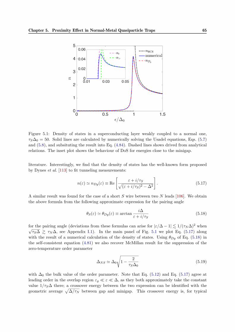
Chapter 5. Proximity Effect in Normal-Metal Quasiparticle Traps 65
Figure 5.1: Density of states in a superconducting layer weakly coupled to a normal one,τS∆0 = 50. Solid lines are calculated by numerically solving the Usadel equations, Eqs. (5.7)and (5.8), and subsituting the result into Eq. (4.84). Dashed lines shows drived from analyticalrelations. The inset plot shows the behaviour of DoS for energies close to the minigap.
literature. Interestingly, we find that the density of states has the well-known form proposedby Dynes et al. [113] to fit tunneling measurements:
n(ε) ' nDy(ε) ≡ Re[
ε+ i/τS√(ε+ i/τS)2 −∆2
]. (5.17)
A similar result was found for the case of a short S wire between two N leads [106]. We obtainthe above formula from the following approximate expression for the pairing angle
θS(ε) ' θDy(ε) ≡ arctan i∆ε+ i/τS
(5.18)
for the pairing angle (deviations from these formulas can arise for |ε/∆− 1| . 1/(τN∆)2 when√τS∆ & τN∆, see Appendix I.1). In the main panel of Fig. 5.1 we plot Eq. (5.17) along
with the result of a numerical calculation of the density of states. Using θDy of Eq. (5.18) inthe self-consistent equation (4.81) we also recover McMillan result for the suppression of thezero-temperature order parameter
∆NS ' ∆0
√1− 2
τS∆0(5.19)
with ∆0 the bulk value of the order parameter. Note that Eq. (5.12) and Eq. (5.17) agree atleading order in the overlap region εg ε ∆, as they both approximately take the constantvalue 1/τS∆ there; a crossover energy between the two expression can be identified with thegeometric average
√∆/τN between gap and minigap. This crossover energy is, for typical

66 Chapter 5. Proximity Effect in Normal-Metal Quasiparticle Traps
Figure 5.2: A non-uniform NS bilayer: a superconducting film of thickness dS (bottom) ispartially covered by a normal metal layer (thickness dN ) occupying the region x > 0. We usethis system to model the vicinity of a normal-metal quasiparticle trap (see text).
parameters, smaller than qubit frequency. Therefore, we can in general use these Dynes-likeformulas as a starting point to evaluate the density of states in a non-homogenous system, aswe show next.
5.3.2 Proximity effect near a trap edge
A normal-metal trap in general covers only part of a superconducting electrode [cf Eq. (3.19)],in order to limit losses in the normal metal that could otherwise shorten the qubit lifetime [75].Typically, traps have lateral dimension of the order of 10 µm or more [47], while the thicknessesdS and dN of superconducting and normal material are in the range of tens of nanometers.These sizes should be compared to the coherence length ξ, which for disordered aluminum filmstypically used to fabricate qubits is of the order of 200 nm. Therefore both the normal andsuperconducting films are thin compared to ξ, while the lateral dimensions of the trap aremuch wider than ξ. We can therefore effectively model the system near the trap edge as beingcomposed by a superconducting film occupying the whole x-y plane and a normal metal in thehalf plane x > 0, see Fig. 5.2.
To study the proximity effect near such an edge, we must allow for spatially dependentparing angles. Due to translational symmetry in the y direction, the derivative with respect toy in Eqs. (4.97) and (4.96) vanishes and we find:
DS
2∂2θS(ε, x)
∂x2 + iε sin θS(ε, x) + ∆(x) cos θS(ε, x)
= 1τS
sin[θS(ε, x)− θN (ε, x)]H(x) ,(5.20)
where DS is the diffusion constant for electrons in the normal state of S and H(x) is the stepfunction [H(x) = 1 for x > 0 and 0 otherwise], and for x > 0
DN
2∂2θN (ε, x)
∂x2 + iε sin θN (ε, x)
= 1τN
sin[θN (ε, x)− θS(ε, x)],(5.21)
with DN the diffusion constant for electrons in N . As before, the superconducting order param-eter ∆(x) is to be found self-consistently using Eq. (4.81). To avoid any confusion, we remind
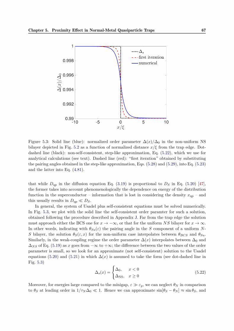
Chapter 5. Proximity Effect in Normal-Metal Quasiparticle Traps 67
Figure 5.3: Solid line (blue): normalized order parameter ∆(x)/∆0 in the non-uniform NSbilayer depicted in Fig. 5.2 as a function of normalized distance x/ξ from the trap edge. Dot-dashed line (black): non-self-consistent, step-like approximation, Eq. (5.22), which we use foranalytical calculations (see text). Dashed line (red): “first iteration” obtained by substitutingthe pairing angles obtained in the step-like approximation, Eqs. (5.28) and (5.29), into Eq. (5.23)and the latter into Eq. (4.81).
that while Dqp in the diffusion equation Eq. (3.19) is proportional to DS in Eq. (5.20) [47],the former takes into account phenomenologically the dependence on energy of the distributionfunction in the superconductor – information that is lost in considering the density xqp – andthis usually results in Dqp DS .
In general, the system of Usadel plus self-consistent equations must be solved numerically.In Fig. 5.3, we plot with the solid line the self-consistent order paramter for such a solution,obtained following the procedure described in Appendix J. Far from the trap edge the solutionmust approach either the BCS one for x→ −∞, or that for the uniform NS bilayer for x→∞.In other words, indicating with θSu(ε) the pairing angle in the S component of a uniform N -S bilayer, the solution θS(ε, x) for the non-uniform case interpolates between θBCS and θSu.Similarly, in the weak-coupling regime the order parameter ∆(x) interpolates between ∆0 and∆NS of Eq. (5.19) as x goes from −∞ to +∞; the difference between the two values of the orderparameter is small, so we look for an approximate (not self-consistent) solution to the Usadelequations (5.20) and (5.21) in which ∆(x) is assumed to take the form (see dot-dashed line inFig. 5.3)
∆s(x) =
∆0, x < 0∆NS, x ≥ 0
(5.22)
Moreover, for energies large compared to the minigap, ε εg, we can neglect θN in comparisonto θS at leading order in 1/τN∆0 1. Hence we can approximate sin[θS − θN ] ≈ sin θS , and

68 Chapter 5. Proximity Effect in Normal-Metal Quasiparticle Traps
at this order Eq. (5.20) decouples from Eq. (5.21). With these approximations, the solution forθS is (cf. Ref. [99])
θS(ε, x) = θL(ε, x)H(−x) + θR(ε, x)H(x) (5.23)θL(ε, x) = θBCS(ε) (5.24)
− 4 arctanexξ
√2α1(ε) tan
[θBCS(ε)− θ0(ε)
4
],
θR(ε, x) = θSu(ε) (5.25)
− 4 arctane−xξ
√2α2(ε) tan
[θSu(ε)− θ0(ε)
4
].
Here, we define the coherence length as ξ =√DS/∆0, introduce the dimensionless functions
α1(ε) =√
∆20 − ε2/∆0 and α2(ε) =
√∆2NS − (ε+ i
τS)2/∆0, and θ0(ε) is the (unknown) value
of θS at the trap edge x = 0. By construction this expression for θS is continuous at x = 0, butit should also be continuously differentiable. Equating the left and right derivatives at the edgegives us a condition that implicitly defines θ0:
√α1(ε)
tan[θBCS(ε)−θ0(ε)
4
]1 + tan2
[θBCS(ε)−θ0(ε)
4
]+
√α2(ε)
tan[θSu(ε)−θ0(ε)
4
]1 + tan2
[θSu(ε)−θ0(ε)
4
] = 0 .
(5.26)
In the weak-coupling regime we are considering, we have α1 ' α2 so long as |ε −∆0| 1/τS .Therefore, except in a narrow energy region near ∆0, Eq. (5.26) has the approximate solution
θ0 '12(θBCS + θSu). (5.27)
Finally, in the energy range where our approximations apply (energy above the minigap andnot too close to ∆0), θSu is well approximated by θDy of Eq. (5.18), which in the same energyrange is close to θBCS . We can therefore linearize Eqs. (5.24) and (5.25) to arrive at
θL(ε, x) ' θBCS(ε)− 12e
xξ
√2α1(ε) [θBCS(ε)− θSu(ε)] (5.28)
θR(ε, x) ' θSu(ε)− 12e−xξ
√2α2(ε) [θSu(ε)− θBCS(ε)] (5.29)
In Fig. (5.4) we compare the density of states obtained from a self-consistent numerical solutionof the Usadel equations (5.20)-(5.21) to an approximate semi-analytic formula which we arrive atby substituting into Eq. (4.84) the Eqs. (5.28)-(5.29) with θSu(ε) found by numerically solvingEqs. (5.7)-(5.8) [or equivalently Eq. (I.3)]. In the next section we will be interested in thespatial evolution of the normalized density of states and pair amplitude away from the normal-metal trap. In order to find an analytic expression for these quantities, we further approximateEq. (5.28) by using the Dynes expression, Eq. (5.18), for θSu and obtain for x < 0 at leading

Chapter 5. Proximity Effect in Normal-Metal Quasiparticle Traps 69
Figure 5.4: Spatial-evolution of quasiparticle density of states for τS∆0 = 100. The density ofstates interpolates between BCS-like form at the right to the bilayer-like form at the left sideof the trap edge. See also Fig. K.2 for Spatial-evolution of pair amplitude.
order (see Appendix K for details)
n(ε, x) ' e−√
2 |x|ξ
(1− ε2
∆20
)1/412
1τS∆0
∆30(
∆20 − ε2)3/2 , (5.30)
p(ε, x) ' e−√
2 |x|ξ
(1− ε2
∆20
)1/412
1τS∆0
ε∆20(
∆20 − ε2)3/2 , (5.31)
for ∆0 − ε 1/τS and ε εg, and
n(ε, x) ' ε√ε2 −∆2
0
− e− |x|
ξ
(ε2∆2
0−1)1/4
1√2
1τS∆0
(5.32)
× ∆30(
ε2 −∆20)3/2 cos
|x|ξ
(ε2
∆20− 1
)1/4
− π
4
,p(ε, x) ' ∆0√
ε2 −∆20
− e− |x|
ξ
(ε2∆2
0−1)1/4
1√2
1τS∆0
(5.33)
× ε∆20(
ε2 −∆20)3/2 cos
|x|ξ
(ε2
∆20− 1
)1/4
− π
4
,for ε −∆0 1/τS . Note that for energies above the gap the corrections to the BCS formulasare always small by construction. Moreover, both above and below the gap the corrections aresmall in 1/τS∆0 and decay exponentially with distance over an energy-dependent length scalewhich is of the order of the coherence length ξ away from the gap, but longer than ξ close to thegap. We have now all the ingredients needed to estimate the quasiparticle-induced transitionrates for a qubit with a trap, which is the focus of the next section.

70 Chapter 5. Proximity Effect in Normal-Metal Quasiparticle Traps
5.4 Qubit relaxation with a trap near the junctionAs discussed in Sec. 5.2, the qubit decay rate due to quasiparticle tunneling is proportional tothe spectral density S, see Eq. (5.1). The spectral density is determined by the quasiparticledistribution function f , the density of states n, and the pair amplitude p, see Eqs. (5.3)-(5.6).We have shown in the previous Section that near a trap n and p become position-dependent.In the next subsection we study how this dependence affects the qubit decay rate, assumingthat quasiparticles are everywhere in thermal equilibrium, so that the distribution function isuniform in space. This assumption is clearly not realistic, since it leads to an increase in thequasiparticle density approaching the trap, but it will enable us to show that the changes inS due to the proximity effect do not significantly harm the qubit if the trap is sufficiently farfrom the junction. In contrast, in Sec. 5.4.2 we will account in a phenomenological way for thespatially dependent suppression of the quasiparticle density caused by the trap. In this morerealistic scenario, we will find an optimal position for the trap, which balances between such asuppression and the enhancement of the subgap density of states, two effects that have oppositeinfluence on the qubit relaxation rate. Throughout this section, we assume that the qubit hasreflection symmetry with respect to the junction, as in experiments [47]; this means that whena trap is mentioned, it should be understood as two identical traps placed at the same distancefrom the junction.
5.4.1 Thermal equilibrium
The assumption of thermal equilibrium means that the distribution function has the Fermi-Diracform,
f eq(ε) = 1eε/T + 1
, (5.34)
with T the quasiparticle temperature. It then follows from Eqs. (5.3)-(5.5) that the spectraldensity obeys the detailed balance relation
Seq(−ω) = e−ω/TSeq(ω) . (5.35)
We assume that the quasiparticles are “cold”, T ω10, and therefore we can neglect the qubitexcitation rate in comparison with the decay rate, since Γeq
01/Γeq10 = e−ω10/T 1.
In presence of a trap, since n and p at the junction position depends on its distance x from thetrap, the quantity A defined in Eq. (5.6) is also a function of x and so is the spectral function. Anapproximate expression for Seq(ω, x) can be obtained in the relevant regime εg T ω ∆0.In practice, since the minigap energy εg is much smaller than temperature, we can set the formerto zero. Then for the quasiparticle tunneling part of the spectral density, we can identify threecontributions (see Appendix L for details on the derivation of the expressions discussed here):
Seqt (ω, x) = Seq
aa(ω, x) + Seqba(ω, x) + Seq
bb (ω, x). (5.36)
The first contribution accounts for transitions in which the initial quasiparticle energy is abovethe gap – then the final energy is also above the gap; this term is approximately independentof position [cf. Eq. (2.45)],
Seqaa(ω, x) ' 8EJ
πxeqqp
√2∆0ω
, (5.37)

Chapter 5. Proximity Effect in Normal-Metal Quasiparticle Traps 71
where xeqqp =√
2πT/∆0e−∆0/T coincides with the equilibrium value of the quasiparticle density
in the absence of the trap. A spatial dependence in principle arises from the corrections termsin Eqs. (5.32) and (5.33), but their contributions can be neglected in comparison with the otherterms in Seq
t which we now discuss.The second term in the right hand side of Eq. (5.36) originates from transitions in which
a quasiparticle initially below the gap absorbs the qubit energy and is excited above the gapenergy:
Seqba(ω, x) ' 8EJ
πxeqqp
√2∆0ω
12τS∆0
e−√
2xξ
(2ω∆0
) 14 ∆0ωeω/T . (5.38)
The small factor 1/τS∆0 and that exponentially decaying with distance account for the smallnessof the initial density of states. In contrast, the final factor is large because the initial occupationprobability is exponentially larger at lower energies. Thus at sufficiently low temperature thisterm can become larger than Saa of Eq. (5.37).
The last term in Eq. (5.36) arises from transitions with both initial and final quasiparticleenergy below the gap,
Seqbb (ω, x) ' 8EJ
π
1(τS∆0)2 e
−2√
2xξ 2 ln 2 T∆0
. (5.39)
Here the small factor 1/τS∆0 is squared, and the exponential decay with distance is faster thanin Eq. (5.38), because both initial and final density of states are small. However, the temperaturedependence is much weaker: Sbb vanishes linearly with T rather than exponentially. Therefore,despite the small prefactors, this term can dominate at low temperatures.
In addition to the single quasiparticle tunneling, pair events can take place. In particular,since the density of states is finite (albeit small) down to the minigap energy εg, so long asω10 > 2εg a pair breaking process is possible, in which the qubit relaxes by breaking a Cooperpair and exciting two quasiparticles above the minigap (but well below the gap). From Eq. (5.5)the spectral density for such a process is (see Appendix L)
Seqp (ω, x) = 8EJ
π
1(τS∆0)2 e
−2√
2xξ
[ω
∆0− 2 ln(2) T∆0
]. (5.40)
The spectral density does not vanish even at T = 0, as there is no need for thermally excitedquasiparticles to be present; in fact, the spectral density decreases linearly with increasing Tbecause the increased occupation of the final states suppresses this process. Interestingly, thislinear in temperature term cancels with Sbb, Eq. (5.39); moreover, while Sba in Eq. (5.38) canbe dominant in the limits of sufficiently small temperature and large distance, its contributionto Seq
t is negligible in the parameter range we are interested in (cf. Fig. 5.5), so that we haveapproximately
Seq(ω, x) ≈ 8EJπ
xeqqp
√2∆0ω
+ 1(τS∆0)2
ω
∆0e−2√
2xξ
. (5.41)
Assuming that the trap is next to the junction, x = 0, in Fig. 5.5 we plot, as functionof temperature, the qubit decay rate Γ10 obtained by substituting Eqs. (5.2) and (5.41) intoEq. (5.1), as well as the contribution from the three type of tunneling processes identified above(above gap to above gap, aa, below gap to above gap, ba and below gap to below gap, bb). At“high” temperature, above about 100 mK but still below the qubit frequency, the dominant con-tribution comes from the position-independent aa term. In contrast, at low temperature there

72 Chapter 5. Proximity Effect in Normal-Metal Quasiparticle Traps
Figure 5.5: Qubit relaxation rate as a function of temperature. We assumed typical transmonparameters for the qubit (see e.g. Ref. [6]): ∆0 = 46GHz, ω10 = 6GHz, EJ = 16GHzand EC = 290MHz; and weak proximity effect, τS∆0 = 103. The solid line (red) shows thetotal relaxation rate, while the other lines show the contributions from the different processesdiscussed in the text.
is a temperature-independent plateau in Γ10 originating from the sum of bb and pair-breakingprocesses. This plateau shows that the trap can increase the decay rate exponentially in com-parison with the no-trap rate, which coincides with the aa term. However, the plateau is quicklysuppressed by moving the trap away from the junction: for each coherence length increase intrap-junction distance, the plateau decreases by a factor e2
√2 ≈ 17. With the parameters of
Fig. 5.5, this means that for x = 4ξ the low-temperature decay rate would be Γ10 < 10−2Hz.Therefore, even though the trap adversely affects the qubit, the limitation imposed on the decayrate becomes quickly negligible by increasing the distance to the junction. The fact that thetrap can only harm the qubit rather than improve its coherence is a consequence of the thermalequilibrium assumption. Next, we relax this assumption to find up to which point the trap canbe beneficial.
5.4.2 Suppressed quasiparticle density
A trap can be beneficial to a qubit primarily by suppressing the quasiparticle density at the junc-tion [68], as discussed in chapter 3. Within the phenomenological diffusion model of Eq. (3.19),the typical length scale over which such a suppression takes place is given by the trapping lengthλtr =
√Dqp/Γeff; this length scale is of order 100 µm [47, 68], much longer than the coherence
length ξ. As for the strength of the proximity effect, based on the experimental parameters of

Chapter 5. Proximity Effect in Normal-Metal Quasiparticle Traps 73
Ref. [47], we estimate it to be τS∆0 ∼ 103-104. The large separation of length scales togetherwith the weakness of normal trap-superconductor coupling, τS∆0 1, make it possible to useEq. (3.19) to calculate the spatial profile of the density, while the modifications introduced bythe proximity effect can be treated as corrections. Below we will consider a realistic device ge-ometry when calculating the position-dependent density, but first we discuss how to incorporatesuch a non-equilibrium quasiparticle configuration into the evaluation of the qubit transitionrates.
When we neglect the proximity effect, the density of states takes the BCS form, Eq. (2.15),and the quasiparticle density defined in Eq. (2.46) can depend on position only through thedistribution function f . Such dependence could arise, for example, due to a temperature pro-file. However, at low temperatures it is in general more appropriate to model non-equilibriumquasiparticles by introducing an effective chemical potential µ [114] (which we measure fromthe Fermi energy). The reason is that recombination processes, which are needed for chemicalequilibrium, are slower than the scattering processes responsible for thermalization [115]. Sucha phenomenological non-equilibrium approach has been already considered in the qubit set-ting [116]. Here to capture the spatial profile of the density we assume the distribution functionf to have the form
f(ε) = 1e(ε−µ)/T + 1
, (5.42)
where the effective chemical potential is a function of position, µ = µ(x), while the effectivetemperature T is homogeneous and does not necessarily coincides with the phonon bath temper-ature. Indeed, typical quasiparticle densities in the absence of traps are in the range xqp ∼ 10−7-10−5, corresponding to effective temperatures (at µ = 0) from ∼ 145mK to ∼ 200mK, muchhigher than both the usual fridge temperature (10-20 mK) and the typical qubit temperaturewhich is of order 35-60 mK [65, 117], as estimated from the excited state population. In the fol-lowing we will present results for T/∆0 in the range 0.01 to 0.05, corresponding to approximately20 mK to 110 mK in aluminum; for a given effective temperature, the chemical potential canthen be calculated by inverting Eq. (2.46) [with n(ε) of Eq. (2.15) and f(ε) of Eq. (5.42)]. So longas e(∆0−µ)/T 1, the integration in Eq. (2.46) gives approximately xqp '
√2πT/∆0e
(µ−∆0)/T
and therefore we find
µ(x) = ∆0 + T ln
√ ∆0
2πTxqp(x)
. (5.43)
The assumption made above gives a restriction on the range of allowed effective temperatures,2πT/∆0 x2
qp, which is however not relevant in practice since usually we have xqp < 10−4 [43]and 2πT/∆0 > 10−2 (since T should be at least comparable to the fridge temperature). Thisrestriction also implies µ < ∆0. We will assume that in general the quasiparticle density xqp(x)is larger than the thermal equilibrium value at temperature T , so that µ > 0. Note that for agiven xqp, µ is a decreasing function of T , while for a fixed T it is an increasing function of xqp.
With the approach described above, given the quasiparticle effective temperature T and thedensity profile xqp(x), one can calculate the effective chemical potential µ(x) using Eq. (5.43)and therefore obtain an expression for the non-equilibrium distribution function, Eq. (5.42).Once the distribution function is known, we can evaluate the spectral density of Eqs. (5.3)-(5.5), which we denote hereinafter with S to remind of its dependence on the non-equilibriumparameters T and µ (and hence on junction-trap distance; we drop in this section the variable x
74 Chapter 5. Proximity Effect in Normal-Metal Quasiparticle Traps
as explicit argument of the spectral density for notational compactness). Similar to the thermalequilibrium case, in the single quasiparticle tunneling contribution St we distinguish three terms:St = Saa + Sba + Sbb. For the first two terms on the right hand side we find, as discussed inAppendix L.0.2, that they are proportional to xqp, as in thermal equilibrium:
Saa(ω) ' 8EJπxqp(x)
√2∆0ω
(5.44)
and
Sba(ω) ' 8EJπxqp(x)
√2∆0ω
12τS∆0
e−√
2xξ
(2ω∆0
) 14 ∆0ωeω/T (5.45)
Here we assume that ω > 0 and ∆0 − µ − ω T ; validity conditions for the approximationsemployed are discussed in more detail in Appendix L.0.2.
For the term Sbb we have different regimes depending on the ratio between ω and µ:
Sbb(ω) ' 8EJπ
1(τS∆0)2×
e−2√
2xξ 2T
∆0ln(
1+eµ/T1+e(µ−ω)/T
), µ . ω
4e−2√
2xξ
(1− µ2
∆20
) 14
∆30(∆2
0+µ2)(∆2
0−µ2)3/2(∆0+µ)3/2×(1√
∆0−µ−ω− 1√
∆0−µ
), µ ω
(5.46)
For this term the similarity with thermal equilibrium is recovered only for µ T . This is thecase also for the pair process contribution Sp:
Sp(ω) ' 8EJπ
1(τS∆0)2 e
−2√
2xξT
∆0
11− e(2µ−ω)/T
×[2 ln 1 + e(ω−µ)/T
1 + e−µ/T− ω
T
] (5.47)
However, a partial cancellation between Sbb and Sp takes place so long as ω−2µ T , in whichcase we find
Sbb(ω) + Sp(ω) ≈ 8EJπ
1(τS∆0)2
ω
∆0e−2√
2xξ , (5.48)
as in thermal equilibrium [compare to the second term in Eq. (5.41)].Turning now to the spectral density at negative frequencies, we note that a relation similar
to Eq. (5.35),St(−ω) = e−ω/T St(ω) (5.49)
follows from Eqs. (5.4) and (5.42). Since we consider ω T , we can neglect the qubit excitationdue to single quasiparticle tunneling. In contrast, for pair processes we find, from Eq. (5.5),
Sp(−ω) = e(2µ−ω)/T Sp(ω) (5.50)
Therefore the rate of qubit excitation induced by quasiparticle recombination can become ex-ponentially larger than qubit relaxation by Cooper pair breaking if 2µ−ω T . We next applythese results to a model of an actual qubit.

Chapter 5. Proximity Effect in Normal-Metal Quasiparticle Traps 75
Figure 5.6: Diagram for the right half of the transmon qubit considered here. Except for theposition of the trap, it is the same design studied in Refs. [47, 68].
5.4.2.1 An example
As a concrete example, we consider the qubit geometry depicted in Fig. 5.6, where a trap withlength d is placed a distance x away from the Josephson junction. Similar geometries have beenused experimentally to measure quasiparticle recombination, trapping by vortices [43] and bynormal-metal traps [47], and theoretically to devise how to optimize trap performance [68]. Herethe only difference is that we allow the long trap, d > l, to be close to the junction, 0 ≤ x ≤ l,so that the role of the proximity effect can be evaluated.
To find the quasiparticle density xqp(x) at the Josephson junction, we proceed as in chapter3 with detail presented in Appendix G.2; we treat each segment of the device (except the padwith side Lpad) as one-dimensional. Since we are interested in the steady-state density, we set∂xqp/∂t = 0 in Eq. (3.19). Solving that equation for each segment of the device, and requiringcontinuity of the density and current conservation at the points where different segments meet,we find
xqp(x) = g
Γeff
1 + 1
sinh(d/λtr)
[ARWλtr
+ cosh(d
λtr
)x
λtr
+ cosh(x+ d− l
λtr
)AcWλtr
]+ 1
2
(x
λtr
)2 . (5.51)
Here AR = W (L+l−x−d)+L2pad is the uncovered area to the right of the trap and Ac = 2WcLc
is the area of gap capacitor. Equation (5.51) makes it clear that the closer the trap is to thejunction, the more the quasiparticle density is suppressed, and that significant changes in thedensity take place over the length scale given by λtr. We can now proceed as outlined above:namely, we first calculate the effective chemical potential µ for different effective temperaturesT . In Fig. 5.7 we show the results of such calculations for two positions of the trap, x = 0 andx = l; hereinafter we use the same realistic parameters for the qubit (L = 1mm, l = 60µm,W = 12µm, Lc = 200µm, Wc = 20µm, Lpad = 80µm) and for the trap (d = 234µm,λtr = 86.2µm) as in Ref. [68], cf. Refs. [43, 47]. We also use the experimentally determinedvalues g = 10−4 Hz [43] and Γeff = 2.42 × 10⁵ Hz [47]. As expected, the effective chemicalpotential decreases with increasing effective temperature, and is larger when the trap is furtheraway.

76 Chapter 5. Proximity Effect in Normal-Metal Quasiparticle Traps
Figure 5.7: The normalized effective chemical potential µ/∆0, see Eq. (5.43), as function of thenormalized effective temperature T/∆0 for two positions of the trap: x = 0 (dashed line) andx = l (solid). The upper effective temperature scale is given for aluminum.
Next, we calculate the qubit transition rates using the thus found chemical potential. Weperform the calculation in two ways: we substitute the chemical potential into Eq. (5.42) forthe distribution function and the latter into the definitions of the spectral functions, Eqs. (5.4)and (5.5); in those equations, we use the semi-analytic results for the pairing angle to determinethe density of states and the pair amplitude, see Eq. (5.28) and the text below Eq. (5.29),and perform the final integration over energy numerically. In a second approach, we use ourapproximate analytical formulas for the spectral functions, see Eqs. (5.44) to (5.50). The ratesso obtained are shown in Fig. 5.8 for an effective temperature T/∆0 = 0.019 (∼ 40mK in Al).In the left panel we distinguish the contributions to 1/T1 due to tunneling-induced relaxation(Γ10,t) and excitation (Γ01,t) and pair process excitation (Γ01,p); the pair process relaxation rateis much smaller than the excitation rate [cf. Eq. (5.50)] and not visible on this scale. In theright panel we plot the total rate 1/T1, which is dominated by the tunneling-induced relaxation;the total rate is a non-monotonic function of trap-junction distance x, due to the competitionbetween processes with initial quasiparticle energy below the gap, whose contributions to therate decay exponentially with distance over a length scale of the order of the coherence length[see Eqs. (5.45) and (5.46)], and processes with above-gap initial energy, with contribution slowlyincreasing with xqp over the much longer length scale λtr. The minimum in this curve thus givesthe optimal position xo for the trap: for x > xo, the density slowly increases, so one is not takingfull advantage of the trap, but at x < xo the subgap density of states quickly increases andnegates the benefit of further density suppression. Therefore we conclude that placing a trap ata distance xo < x < λtr represents the best choice. In Fig. 5.9 we further explore the dependenceof the optimal position xo on parameters such as the effective temperature T and the strength ofthe proximity effect τS∆0 (we remind that the larger this parameter, the weaker the proximity

Chapter 5. Proximity Effect in Normal-Metal Quasiparticle Traps 77
Figure 5.8: Left: tunneling (t) and pair (p) contributions to the qubit decay rate 1/T1 as afunction of trap-junction distance x (the pair decay rate Γ10,p is too small to be visible). Theeffective temperature is T/∆0 = 0.019 (approximately 40 mK in Al), other parameters are as inFig. 5.5. The solid lines have been obtained by numerically calculating the integrals determiningthe spectral functions, while the dashed lines are our approximate analytical findings (see textfor more details). Right: Total qubit decay rate, showing a minimum for a distance of a fewcoherence lengths.
effect). Clearly, the stronger the proximity effect, the further a trap should be placed. As theeffective temperature increases, on the other hand, the optimal position decreases: as alreadynoted before, for a given density the higher the effective temperature, the smaller the effectivechemical potential, and this reduces the importance of the subgap states, since their occupationdecreases. Based on this figure, we conclude that when the distance is over 20 coherence lengthsthe proximity effect can be safely neglected; in aluminum such a distance is of the order of afew microns, which is still much less than the trapping length.
5.5 Summary
In this work we investigate the proximity effect between a normal-metal quasiparticle trap andthe superconducting electrode of a qubit. On one hand, a trap can prolong the relaxationtime of the qubit by suppressing the quasiparticle density. On the other hand, the proximityeffect induces subgap states which can shorten the relaxation time. To quantify the competitionbetween these two phenomena, we start by considering a uniform superconductor-normal metalbilayer; at relevant energies, the density of states takes the Dynes form, Eq. (5.17), with thebroadening determined by interface resistance, superconducting film thickness, and its densityof states at the Fermi energy. We then study how such broadening decays away from a trap edge,

78 Chapter 5. Proximity Effect in Normal-Metal Quasiparticle Traps
Figure 5.9: Normalized optimal trap-junction distance xo/ξ as a function of normalized effectivetemperature T/∆0 (the upper scale gives the corresponding temperature for aluminum). Solid(dashed) lines are obtained by numerically finding the position of the minimum in curves suchas the solid (dashed) one in the right panel of Fig. 5.8.
see Eqs. (5.30) to (5.33). With these results, we can evaluate the qubit decay rate as function ofthe distance between trap and junction; we take into account the suppression of the quasiparticledensity by introducing a distribution function which depends on two parameters, an effectivetemperature and a distance-dependent effective chemical potential, cf. Eq. (5.42). Withinthis approach, we find that the competition between proximity effect and density suppressionleads to an optimal placement for the trap, see Figs. 5.8 and 5.9. The qubit relaxation rateexponentially increase for a trap closer to the junction than this optimum over a length scale ofthe order of the coherence length, while the increase of the rate when moving the trap fartheraway is much slower and over the much longer trapping length. Therefore, a trap should beplaced at least as far from the junction as the optimum position, but no significant penalty ispaid for distances up to the trapping length.
While we focused here on a transmon qubit, our findings may prove useful in designing trapsfor other systems as well. For example, quasiparticle poisoning could be a significant hurdle fornanowire-based realization of Majorana qubits [27]; our findings indicate that a normal-metaltrap placed close to the ends of the nanowire could be detrimental, as the small minigap isnot sufficient to protect zero-energy states from being thermally excited into the subgap statesinduced by the trap. Finally, our results on the proximity effect could also help interpretingtunneling density of state experiments such as those reported in Refs. [100, 118]

Chapter 6
Summary and Conclusions
Quasiparticle tunneling is an intrinsic decoherence channel for superconducting qubits with acorresponding relaxation rate that linearly scales with the density of quasiparticles present atclose vicinity of qubit Josephson junction. While the generation mechanism of non-equilibriumquasiparticles at millikelvin temperatures is still an open question, in this thesis we focusedon manipulating quasiparticle population to limit and reduce harmful consequences of theirpresence. We studied how a normal-metal in tunnel contact with a superconductor can trapquasiparticle excitations. We showed these traps can be beneficial for superconducting qubitsin three ways: first, suppressing the steady-state quasiparticle density at the junction that canimprove qubit’s T1 time. Second, a trap can speed up the decay of the excess quasiparticlesand, third, it can decrease fluctuations around the steady-state density; these effects of normal-metal quasiparticle traps are promising to achieve longer-lived qubits that are also more stablein time.
We developed a phenomenological diffusion equation that explains the effect of a normal-metal trap on the dynamics and steady-state of non-equilibrium quasiparticle population in asuperconducting qubit. The model takes into account the tunneling between the superconductorand the trap, as well as the electron energy relaxation in the trap, see Eq. (3.18). Due to thepronounced energy dependence of quasiparticle density of states for energies above and close tothe gap, the effective trapping rate Γeff becomes sensitive to the energy of the quasiparticles andis limited by their backflow from the normal-metal trap on time scales shorter than the electronenergy relaxation rate. Furthermore, we find how the time needed to evacuate the injectedquasiparticles depends on the trap size. This evacuation time saturates at the lowest, diffusion-limited value upon extending the trap above a certain characteristic length l0. To supportour theory, we reported experimental data (obtained by our collaborators) that confirms thepredictions of our model. For small traps we can estimate the effective trapping rate Γeff:both its order-of-magnitude and its increase with temperature indicate a limitation due to thebackflow of quasiparticles.
The bottleneck for trapping is confirmed to be slow energy relaxation inside the trap; thisquantity is very difficult to manipulate. In order to improve trapping efficiency, we studied theeffects of size, number and position of quasi-1D normal-metal traps. We prefer 1D traps over2D traps because 2D traps are strong only if they are large compared to the trapping lengthλtr of Eq. (3.21), while in quasi-1D it is sufficient for the trap length d to be longer than thecharacteristic scale l0 [Eq. (3.34)] that is generally shorter than λtr for long devices (Ldev > λtr).We point out that covering a large part of the qubit by a normal-metal trap could be a sourceof unwanted dissipation that harms qubit coherence.
For a weak trap (d . l0), the trap position has a negligible effect on the ability to suppressquasiparticle density and its fluctuations, as well as on the decay rate of excess quasiparticles.In contrast, we find a number ways to optimize a strong but short trap, l0 . d . λtr. First,

80 Chapter 6. Summary and Conclusions
placing a single trap at the optimum position that makes the decay of excess quasiparticles asfast as possible, see Figs. 3.7 and 3.8. We found that in general it is advantageous to dividea strong trap into smaller pieces of length ∼ l0 and distribute those around the device, seeSec. 3.2.2.2. Second, we find that there is an optimal trap position for suppressing densityfluctuations, see Sec. 3.2.3.1. In addition, we find that there is a maximum distance Lf fromthe junction up to which the suppression of fluctuations is effective; this distance is smallerthan the distance where, for a given trap size, large suppression of the steady-state density isachieved. Therefore, suppressing fluctuations by a normal-metal trap indicates that the steady-state density is suppressed as well. These lead us to the conclusion that by correctly placingmultiple traps in the device in such a way that one is sufficiently close to the junction, all threebeneficial effects of traps can be optimized.
In addition to trapping quasiparticles, a normal-metal material in contact with a super-conductor has a number of side effects that can influence qubit performance. In particular,Cooper-pairs leak to the trap as well, and this leads to modifications in superconducting prop-erties. We used Usadel formalism to study this effect. We find proximity-induced subgap densityof states in the superconducting electrode from both self-consistent numerical and analyticalapproaches; see Figs. 5.1 and 5.4. This subgap density of states modifies quasiparticle tunnelingcontribution in the total decay rate and can open up new decay channel due to pair processes.In order to find the qubit relaxation rate, we modeled quasiparticle distribution function byuse of the diffusion model that we developed earlier; see Eqs. (5.42) and (5.43). While thequasiparticle density is more suppressed by moving the trap closer to the junction, the mag-nitude of trap-induced subgap density of state becomes exponentially enhanced. This leads toa non-monotonic relation for the qubit relaxation as a function of trap-junction distance, Fig.(5.8). Our analysis has enabled us to find up to which point in trap-junction distance a trap canbe beneficial to the qubit coherence; depending on temperature and resistance at the qubit-trapcontact, one needs to place the trap of order 4 to 20 coherence lengths away from the junctionin order to prevent proximity effect from harming the qubit coherence; see Fig. 5.9. Placing thetrap further away from the junction than this optimum up to the “trapping length” does notsignificantly increase the qubit decay rate.
We stress that our considerations for normal-metal quasiparticle trapping are valid for nor-mal islands in tunnel contact with the superconductor. A good contact between the qubit anda normal metal or another superconductor with a lower energy gap can also act as a trap bylocalizing the quasiparticles away from the junction. Studying such trapping scenarios basedon band-gap engineering is an important topic, but it is beyond the scope of the present thesis.

Appendix A
Tunneling rate equations
In this Appendix, we derive the rate equations for quasiparticles and electrons accountingfor tunneling between a superconductor and a normal metal. Here we assume that both thesuperconductor and the normal metal are sufficiently small volumes (ΩS and ΩN , respectively),such that the diffusion of excitations occurs on a fast time scale and the occupation probabilitiesare hence uniform in space. Within these volumes we define the probabilities
f (ξm) =∑σ
⟨c†mσcmσ
⟩(A.1)
fqp (εn) =∑σ
⟨γ†nσγnσ
⟩(A.2)
of finding an electron excitation of energy ξm in the normal metal and a quasiparticle excitationof energy εn in the superconductor, respectively. The tunnel coupling between the two, seeEq. (3.4), gives rise to a change in both occupation probabilities for energies above the gap, viaprocesses whose rates can be computed using Fermi’s Golden Rule:
f (ξm) =∑nσ
[Wnσ→mσ −Wmσ→nσ +W0→mσ,n−σ −Wmσ,n−σ→0] , (A.3)
fqp (εn) =∑mσ
[−Wnσ→mσ +Wmσ→nσ +W0→mσ,n−σ −Wmσ,n−σ→0] , (A.4)
with
Wnσ→mσ =2π~
∣∣∣t∣∣∣2ΩSΩN
u2nfqp (εn) [1− f (ξm)] δ (εn − ξm) , (A.5)
W0→mσ,n−σ =2π~
∣∣∣t∣∣∣2ΩSΩN
v2n [1− fqp (εn)] [1− f (ξm)] δ (εn + ξm) . (A.6)
The reverse processes are found by replacing f(qp) → 1−f(qp). Assuming particle-hole symmetry,f (−ξ) = 1− f (ξ), we summarize the rate equations as
f (ξm) =2π~
∣∣∣t∣∣∣2ΩSΩN
∑n
[fqp (εn)− f (ξm)] δ (εn − ξm) (A.7)
fqp (εn) =2π~
∣∣∣t∣∣∣2ΩSΩN
∑m
[f (ξm)− fqp (εn)] δ (εn − ξm) . (A.8)
The tunneling processes considered above are elastic. In the normal metal, for temperaturesT ∆ there is a large interval of unoccupied states below the gap. Inelastic processes, suchas electron-phonon and electron-electron interactions, can relax the excitations in the normal
82 Appendix A. Tunneling rate equations
metal to energies below the gap, so that they cannot return to the superconductor. We phe-nomenologically account for this relaxation by adding the term −Γrf (ξm) to the right-handside of Eq. (A.7). The relaxation rate Γr is assumed energy-independent, which is justified ifthe interval of non-zero excitations above the gap is within a narrow energy strip of width ∆.
In the next step, we are interested in the probabilities to find excitations in the states withina small energy interval δε. We define the probability densities
pN (ε) = 1NS
∑ε<ξm<ε+δε
f (ξm) (A.9)
pS (ε) = 1NS
∑ε<εn<ε+δε
fqp (εn) (A.10)
which are normalized with respect to the normal-state number of states in the superconductorNS = νS0ΩSδε. In the continuum limit δε→ 0 these definitions lead to Eqs. (3.12) and (3.13),respectively. From Eqs. (A.7)-(A.8) plus the phenomenological relaxation term discussed above,we obtain Eqs. (3.15)-(3.16) with the rates
Γesc (ε) = 2π~
∣∣∣t∣∣∣2 νS0ΩN
ε√ε2 −∆2
, (A.11)
Γtr = 2π~
∣∣∣t∣∣∣2 νN0ΩS
. (A.12)

Appendix B
Derivation of effective trapping rate
In this Appendix we provide a derivation of the effective trapping rate, including diffusion.It is a straightforward continuation of the rate equation derived in the previous Appendix A.In disordered metals, the effect of elastic impurity scattering on the distribution function isaccounted for by a diffusion term; for quasiparticles in superconductor, the diffusion constantin the so-called “hydrodynamical approach” [66] is energy-dependent:
pN (ε, ~r, t) =DN~∇2pN (ε, ~r, t) + δ (z − tS) [γtrpS (ε, ~r, t)
−γesc (ε) pN (ε, ~r, t)]− ΓrpN (ε, ~r, t) (B.1)
pS (ε, ~r, t) =DS (ε) ~∇2pS (ε, ~r, t)− a (x, y) δ (z − tS)× [γtrpS (ε, ~r, t)− γesc (ε) pN (ε, ~r, t)] . (B.2)
In this Appendix, we disregard recombination and background terms for the quasiparticlesthat may in general appear. Those are taken into account in the main text. The above isa set of coupled linear equations that can be solved analogously to the solution in the maintext in terms of eigenmodes with corresponding eigenmodes. The only difference is that here,we keep the energy argument. Since all the processes but the relaxation term are elastic,the equations at different energies are uncoupled and we can find independent eigenmodes ateach energy ε. The diffusion constant in the superconductor is in general energy dependent,DS (ε) =
√ε2−∆2
ε DS (∞) (valid for dirty superconductors). We will first derive an effectivetrapping rate for each energy and provide the conditions of validity. In a second step, weprovide the effective rate for the quasiparticle density xqp when integrating over ε.
B.1 Thin normal metalFirst, we assume a sufficiently thin trap such that the electron density within the normal metaldoes not change significantly in z-direction. This is true if the length scale, on which pN decaysin z, λr, is much larger than the thickness of the trap, tN λr. We may prove this along thefollowing lines. The diffusion equation for the normal metal may be alternatively expressed as
pN (ε, ~r, t) = DN~∇2pN (ε, ~r, t)− ΓrpN (ε, ~r, t) (B.3)
for z > tS , with the boundary condition at z = tS
DN∂zpN (ε, x, y, tS , t) + γtrpS (ε, x, y, tS , t)− γesc (ε) pN (ε, x, y, tS , t) = 0 . (B.4)
We make the following ansatz, assuming that pN is almost constant in z direction,
pN (ε, ~r, t) = pN (ε, x, y, t) + (z − tN − tS)2
2t2NdpN (ε, x, y, t) . (B.5)

84 Appendix B. Derivation of effective trapping rate
The term proportional to dpN corresponds to the next-to-leading order correction. There areno linear terms in z− tN − tS in this expansion, as to respect the hard wall boundary ∂zpN = 0at z = tS + tN . Above expansion is well-defined if dpN pN . Plugging this ansatz into abovediffusion equation, we get the equation in leading order
˙pN = DN~∇2pN + DN
t2NdpN − ΓrpN . (B.6)
For the boundary condition we obtain likewise in leading order
−DN
tNdpN + γtrpS − γesc (ε) pN = 0 . (B.7)
We reinsert this into the diffusion equation, and we obtain
˙pN = DN~∇2pN + 1
tN[γtrpS − γesc (ε) pN ]− ΓrpN . (B.8)
Note that the boundary condition in leading order relates the correction dpN to pS and pN , andthus provides the limit of validity of the thin film approximation,
tN DN
γtrpSpN− γesc (ε) . (B.9)
This condition can be evaluated when formally solving Eq. (B.8), in order to relate the time-evolution of pN to pS . This equation has a set of eigenmodes, which are discrete due to thefinite size of the normal metal. Choosing the coordinate system such that the metal has itshard wall borders at x = 0, dx, y = 0, dy, we find eigenmodes of the form
n(kx, ky) =√NxNy cos(kxx) cos(kyy) , (B.10)
with kx,y = πnx,y/dx,y, nx,y ∈ N, the normalisation constant Nx,y = 1 + δ0nx,y , and the corre-sponding eigenvalues
λ(kx, ky) = −DNk2x −DNk
2y − Γesc(ε)− Γr . (B.11)
This allows us to express the solution of the normal metal density distribution as
pN (x, y, t) = − γtrtN
∫dω
2π∑kx,ky
e−iωt
iω + λ(kx, ky)n(kx, ky)pS(kx, ky, ω) , (B.12)
with the Fourier-transformed density in the superconductor
pS(kx, ky, ω) =∫ dx
0
dx
dx
∫ dy
0
dy
dyn(kx, ky)×
∫dteiωtpS(x, y, t) . (B.13)
In the solution given in Eq. (B.12) we discarded any transient terms, which are exponentiallysuppressed for times t (Γesc(ε) + Γr)−1. Assuming that pS has some cutoff in k-space andfrequency space, i.e., pS varies on a maximal length scale λS and time scale τS , we may, bymeans of Eqs. (B.12) and (B.13) approximate
pSpN∼ τ−1
S +DNλ−2S + Γesc(ε) + Γr . (B.14)

Appendix B. Derivation of effective trapping rate 85
Hence we find the general condition for the thickness of the normal metal
tN √
DN
τ−1S +DNλ
−2S + Γr
. (B.15)
In the next section, we consider the case when pS varies sufficiently slowly in space and time,where it is sufficient that
tN √DN
Γr. (B.16)
B.2 Effective trapping rateThe next crucial step involves the assumptions, that pS varies sufficiently slowly in x, y, andt, such that we can neglect the terms pN and ~∇2pN . Let us for now just denote the time andspatial scales at which pS changes as τS and λS , and identify them later. We may approximate
pN (ε, x, y, t) ≈ γtrtN
1Γesc (ε) + Γr
pS (ε, x, y, tS , t) + dpN (ε, x, y, t) (B.17)
where the second term on the right hand side merely represents the correction, which has to besmall, dpN pN . Inserting the approximated pN into the diffusion equation for pS , we find
pS (ε, ~r, t) = DS (ε) ~∇2pS (ε, ~r, t)− a (x, y) δ (z − tS) γeff (ε) pS (ε, ~r, t) (B.18)
with
γeff (ε) = γtrΓr
Γesc (ε) + Γr. (B.19)
As mentioned before, for above equation to be valid, we require dpN/pN 1, through whichwe find that the temporal variation of pS has to satisfy
Γesc (ε) + Γr τ−1S (B.20)
and the spatial variation must fulfill√Γesc (ε) + Γr
DN λ−1
S . (B.21)
We are now left with identifying the scales τS and λS . We do it explicitly for the experimentallyrelevant specific example of a thin superconductor where, pS likewise varies slowly in z withrespect to the thickness tS . In analogy to the normal metal case in the previous section, the zdependence may likewise be neglected if tS
√DS (ε) /Γeff (ε), for Γeff = γeff/tS . Through the
inequality
DS (ε)Γeff (ε) ≥
DS (∞) Γesc (∞)ΓtrΓr
(B.22)
we find the sufficient condition
tS
√DS (∞) Γesc (∞)
ΓtrΓr. (B.23)

86 Appendix B. Derivation of effective trapping rate
For tS ≈ tN and νS0 ≈ νN0, this condition reduces to tS √DS (∞) /Γr. For a thin supercon-
ductor, we obtain likewise the diffusion equation
pS (ε, x, y, t) = DS (ε) ~∇2pS (ε, x, y, t)− a (x, y) Γeff (ε) pS (ε, x, y, t) . (B.24)
From this equation, we now estimate the time scale and spatial scale on which pS varies. Namely,for a superconductor much larger than the normal metal trap, d L (where d and L denotethe length scales of trap and superconductor, respectively), the time scale at which pS relaxesis maximally given by the diffusion time (see also main text),
tS ∼L2
DS (ε) . (B.25)
Underneath the trap, the density pS changes spatially on a length scale given by the trappinglength,
λS = λtr ∼√DS (ε)Γeff (ε) . (B.26)
With these two results we find the conditions of validity for the effective trapping rate,
Γesc (ε) + Γr DS (ε)L2 (B.27)
and
(Γesc (ε) + Γr)2
ΓtrΓr DN
DS (ε) . (B.28)
From the former condition, we find through Γesc (ε) ≥ Γesc (∞) and DS (ε) ≤ DS (∞), thesufficient condition
Γesc (∞) + Γr DS (∞)L2 . (B.29)
The latter condition is a bit less trivial to analyse. First we transform it into(Γesc (∞)
√ε
(ε2−∆2)14
+ Γr(ε2−∆2)
14
√ε
)2
ΓtrΓr DN
DS (∞) . (B.30)
Here we see that the left hand side is in general a non-monotonic function of ε. We may howevercompute the minimum of the left hand side as a function of the ratio Γesc (∞) /Γr, in order toderive a sufficient condition. We differ between two cases. For
Γesc (∞)Γr
≥ 1 (B.31)
the minimum is at ε ∆. As in our considerations the quasiparticle occupation is nonzeroonly for an energy window dE = ε−∆ ∆, this minimum is irrelevant, and we find for ε closeto ∆
Γ2esc (∞)ΓtrΓr
1√2
√∆
ε−∆ DN
DS (∞) (B.32)

Appendix B. Derivation of effective trapping rate 87
which is fulfilled as long as
dE
∆ 12D2S (∞)D2N
(Γ2esc (∞)ΓtrΓr
)2
. (B.33)
For instance for DS ∼ DN and Γesc (∞) ∼ Γtr ∼ Γr, above inequality is always fulfilled. For
Γesc (∞)Γr
< 1 (B.34)
on the other hand, the minimum is located at
ε−∆∆ = 1
2Γ2esc (∞)
Γ2r
. (B.35)
Hence here, the minimum becomes only relevant for Γesc (∞) Γr. In such a case we wouldfind the condition
4Γesc (∞)Γtr
DN
DS (∞) , (B.36)
This case is however not relevant for the experimental parameters, as there we have Γesc (∞) ona similar order of magnitude as Γr. And even if Γesc (∞) Γr, the backflow of quasiparticles isnot important, making a formulation for an effective trapping rate including backflow redundantright from the start.
B.3 Effective trapping rate integrated over energyEventually, we consider the normalised quasiparticle density xqp = 2
∆∫∞
∆ dεpS (ε). Integratingthe diffusion equation, Eq. (B.18), over ε, we get
xqp = Dqp~∇2xqp − a(x, y)δ(z − tS)γeffxqp (B.37)
where the notation is chosen such that the γeff without energy argument corresponds to theeffective trapping rate integrated over energies, i.e.,
γeff =∫∞
∆ dεγeff (ε) pS (ε)∫∞∆ dεpS (ε) . (B.38)
Likewise, the 2D diffusion equation for thin superconductors, Eq. (B.24), may be integrated,
xqp = Dqp~∇2xqp − a(x, y)Γeffxqp (B.39)
where here, xqp depends only on x and y, and Γeff = tS γeff. Recalling that pS (ε) = ε√ε2−∆2 fqp (ε),
we now assume that quasiparticles of high energies relax fast to energies close to the gap, suchthat fqp = 0 above a certain threshold energy ε = ∆ + dE, where dE ∆. Disregarding thedetailed energy dependence of fqp below this threshold, we find
Γeff ≈ Γtr
∫∆+dE∆ dε Γr
Γesc(ε)+Γr
√∆ε−∆∫∆+dE
∆ dε√
∆ε−∆
. (B.40)

88 Appendix B. Derivation of effective trapping rate
We may easily evaluate this integral, in two limits. For
Γesc (∞)Γr
√dE
∆ (B.41)
we receive
Γeff ≈1√2
ΓtrΓrΓesc (∞)
√dE
∆ . (B.42)
For
Γesc (∞)Γr
√dE
∆ (B.43)
on the other hand we get
Γeff ≈ Γtr (B.44)
that is, in this case, the backflow of quasiparticles is irrelevant. Phenomenological equationssuch as Eq. (B.39) are widely used in the literature [53, 54, 43, 25, 56, 67] as they successfullydescribe experiments as in Sec. 3.1.4.

Appendix C
Comparison with vortex trapping
In the coplanar gap capacitor transmon, the antenna pads are the widest part of the device.This makes it possible to trap vortices only in the pads when cooling the device in a smallmagnetic field. It was shown in [43] that each vortex added to a pad increases the density decayrate, and the effectiveness of trapping by vortices was characterized by a “trapping power” P .Here we compare the vortex trapping with a normal-metal trap covering the pad. To determinethe decay rate of the excess density xqp, we construct the solution to the diffusion equation(3.19), along the lines of the Supplementary to Ref. [43]. We treat all parts of the deviceexcept the pad as one-dimensional and write xqp in each segment in the form of Eq. (3.46). Weapproximate the density in the pad as uniform (justified for the lowest mode if Lpad < λeff, as inthe actual devices). We then impose continuity of the density and current conservation wherethe parts of the device meet and thus arrive at the following effective boundary condition forthe density at the connection between wire and pad (at y = L):
∂xqp∂y
∣∣∣y=L
= L2pad
[Dqpk
2 − ΓeffWDqp
]xqp(y = L) . (C.1)
Let us introduce for simplicity the dimensionless parameter z = kL; after imposition of allboundary conditions, as detailed in [43], we find that the parameter must satisfy the equation
(L2
padΓefftL
LW
)[1− f(z) tan z]− z[tan z + f(z)] = 0 , (C.2)
with tL = L2/Dqp and (see Ref. [43])
f(z) = tan(zl
L
)+ 2Wc
Wtan
(zLcL
). (C.3)
The similar calculation for the case of N vortices in each pad leads to the following equationfor z: (
NP tLLW
− az2)
[1− f(z) tan z]− z[tan z + f(z)] = 0 (C.4)
with a = L2pad/(LW ); since in the experiments the latter quantity as well as z for the lowest
mode and the coefficient multiplying N are all of order unity, in this equation we can neglectthe term proportional to a for large number of vortices. Then, by comparing Eq. (C.2) toEq. (C.4) we immediately see that for the vortex trapping to generate the same decay rate asthe normal-metal trap, the number of vortices in each pad must be equal to:
N =L2
padΓeff
P(C.5)

90 Appendix C. Comparison with vortex trapping
Using P = 6.7× 10⁻²cm2 s−1 and Lpad = 80 µm [43], the number of vortices in each pad wouldneed to be N ' 230. This shows that many vortices are needed to match the efficiency of thenormal metal trap.
The cooling magnetic field needed to achieve this vortex number can be estimated to beB ∼ NΦ0/Spad ∼ 0.75 G, well into the regime in which the dissipation caused by the vorticesnegatively affect the qubit coherence [43]. A normal-metal island could also lead to dissipation.However, solving Eq. (C.2) for the parameters specified in Fig. 3.7, we find a density decay rateτ−1w ≈ 1.7ms−1 for a metal-covered pad. From Fig. 3.7 we see that an optimally placed trap oflength comparable to l0 can achieve this decay rate, even though the trap area is much smallerthan the pad area – thus, optimal placement can potentially limit the losses due to the normalmetal.

Appendix D
Finite-size trap
In this appendix, we treat a 1D system with a finite-size trap to identify the regime in which itcan be considered as infinitely small. Moreover, we describe the crossover from infinitely smallto finite size trap in the strong trapping regime.
We consider the 1D diffusion equation (where the spatial coordinate is 0 ≤ y ≤ L)
xqp = Dqp∇2xqp −A (y) Γeffxqp. (D.1)
We model the trap as a piece of length d, starting from y = 0, i.e., A (y) = 1 for y ≤ d and 0otherwise, see Fig. D.1(a). Since no quasiparticle can leave the ends of the 1D wire, we adopt“hard wall” boundary conditions [76]
∂xqp∂y
∣∣∣y=0
= ∂xqp∂y
∣∣∣y=L
= 0 . (D.2)
The time-dependent solution of this problem can be expressed through the decompositioninto eigenmodes, where
xqp (y, t) =∑k
eµktαknk (y) (D.3)
and the eigenmodes fulfill
µknk (y) =[Dqp~∇2 −A (y) Γeff
]nk (y) . (D.4)
The eigenvalue problem can be solved with the Ansatz
nk (y) = 1√Nk
cos
(ky), y < d
ak cos (ky) + bk sin (ky) , y > d(D.5)
which satisfies the first boundary condition in Eq. (D.2) and we defined
k =√k2 − λ−2
tr , (D.6)
with λtr of Eq. (3.21) and Nk is a normalization constant. From this Ansatz it follows thatµk = −Dqpk
2. Continuity of the function nk and its derivative at y = d, together with thesecond condition in Eq. (D.2), provide an equation for k:
k tan [k (L− d)] = −k tan(kd). (D.7)
While the modes thus defined provide the full time-evolution for all times, we are usuallyinterested in the lowest mode which dominates the long-time behavior and which we denotewith k0. Assuming k0 λ−1
tr , we have k0 ≈ 1/λtr and we may approximate Eq. (D.7) as
leffk = cot [k (L− d)] , (D.8)
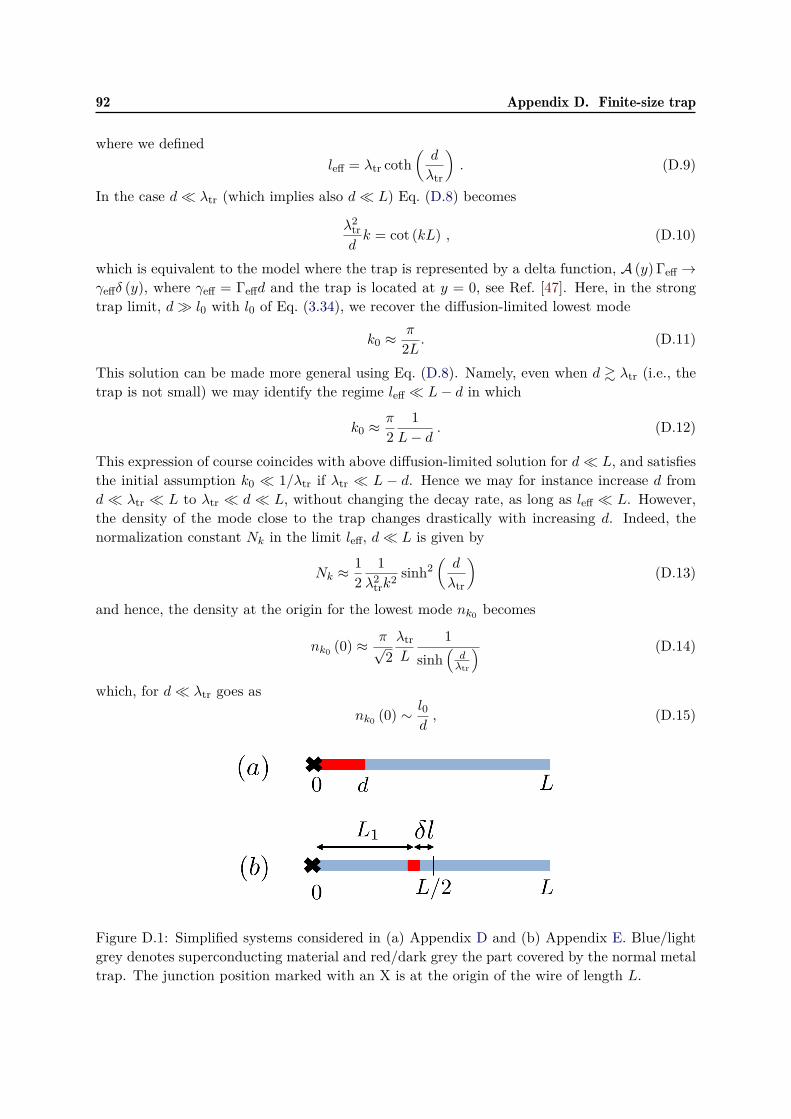
92 Appendix D. Finite-size trap
where we definedleff = λtr coth
(d
λtr
). (D.9)
In the case d λtr (which implies also d L) Eq. (D.8) becomes
λ2trdk = cot (kL) , (D.10)
which is equivalent to the model where the trap is represented by a delta function, A (y) Γeff →γeffδ (y), where γeff = Γeffd and the trap is located at y = 0, see Ref. [47]. Here, in the strongtrap limit, d l0 with l0 of Eq. (3.34), we recover the diffusion-limited lowest mode
k0 ≈π
2L. (D.11)
This solution can be made more general using Eq. (D.8). Namely, even when d & λtr (i.e., thetrap is not small) we may identify the regime leff L− d in which
k0 ≈π
21
L− d. (D.12)
This expression of course coincides with above diffusion-limited solution for d L, and satisfiesthe initial assumption k0 1/λtr if λtr L − d. Hence we may for instance increase d fromd λtr L to λtr d L, without changing the decay rate, as long as leff L. However,the density of the mode close to the trap changes drastically with increasing d. Indeed, thenormalization constant Nk in the limit leff, d L is given by
Nk ≈12
1λ2trk
2 sinh2(d
λtr
)(D.13)
and hence, the density at the origin for the lowest mode nk0 becomes
nk0 (0) ≈ π√2λtrL
1sinh
(dλtr
) (D.14)
which, for d λtr goes asnk0 (0) ∼ l0
d, (D.15)
Figure D.1: Simplified systems considered in (a) Appendix D and (b) Appendix E. Blue/lightgrey denotes superconducting material and red/dark grey the part covered by the normal metaltrap. The junction position marked with an X is at the origin of the wire of length L.

Appendix D. Finite-size trap 93
while for d λtr we findnk0 (0) ∼ λtr
Le− dλtr . (D.16)
As we see, by increasing d above the trapping length scale λtr, the density of quasiparticles getsexponentially suppressed near the trap. For a long trap d λtr, such an exponential suppressiontakes place also for the steady-state density, as one can verify by reintroducing the generationrate g in the right hand side of Eq. (D.1) and solving for the steady-state configuration withxqp = 0.


Appendix E
Quasi-degenerate modes and theirobservability
In this appendix, we consider the dependence of the lowest mode on the trap position. More-over, we show that close to the optimal position the lowest and second lowest modes arequasi-degenerate. We finally comment on the consequences of this quasi-degeneracy on theobservability of the lowest mode.
We take for simplicity a small trap (d λtr) in a wire of length L, placed at an arbitrarydistance l from the origin; the quasiparticle density then obeys the diffusion equation (see [47]and App. D)
xqp = Dqp~∇2xqp − δ (y − l) γeffxqp. (E.1)
To solve this equation, we look for eigenmodes nk that must satisfy at y = l the condition
lsat[∂yn
+k (l)− ∂yn−k (l)
]= nk (l) (E.2)
with lsat =√Dqptsat, where tsat = Dqp/γ
2eff, and the short-hand notation ∂yn±k (l) = ∂ynk|y=l±0+ .
The saturation time tsat was introduced in Eq. (3.31) when studying the quasiparticle dynamicsduring injection and gives the time scale to reach a steady state. Here we use the related lengthsscale lsat to have a more compact notation: due to the identity
π
2lsatL
= l0d, (E.3)
this is not an independent parameter in the problem, and the strong (weak) trap condition canbe expressed as lsat L (lsat L).
Assuming “hard walls” on both ends, ∂ynk(0) = ∂ynk(L) = 0, the eigenmodes are given by
nk =
ak cos (ky) for y < l
bk cos (k [L− y]) for y > l. (E.4)
These mode decay with a rate 1/τk = Dqpk2. From Eq. (E.2) and continuity of nk, we find the
condition for klsatk sin (kL) = cos (kl) cos (k [L− l]) . (E.5)
For an infinitely strong trap, lsat → 0, we get the condition
cos (kl) cos (k [L− l]) = 0, (E.6)
which provides for the lowest mode either k = π2l or k = π
2[L−l] depending on whether L− l ≷ l.Note that the continuity of the modes at y = L1 requires
ak cos (kl) = bk cos (k [L− l]) (E.7)

96 Appendix E. Quasi-degenerate modes and their observability
which means that bk = 0 for k = π2l or likewise ak = 0 for k = π
2[L−l] . In other words, the trapeffectively separates the wire into two independent pieces, one to the left and one to right of thetrap, with the quasiparticle density of the lowest mode fully suppressed in the shorter piece.
We define the optimal trap position as the one where the lowest mode decay rate is thehighest. It is easy to see that this is at the degeneracy point, l = L/2, where the two modes’decay rates coincide. Note however, that when passing the degeneracy point by increasing l froml < L/2 to l > L/2, the eigenmode function jumps abruptly from being nonzero on the righthand side to nonzero on the left. Therefore, whether the quasiparticle density actually decayswith the rate defined by the lowest mode, can be strongly affected by the initial conditions. Inorder to study this effect, we depart from the ideal, infinitely strong trap, and take a small butfinite lsat. In addition, we look at a system close to the degeneracy point, that is, l = L/2 + δl
with δl L/2. We first expand Eq. (E.5) for small δl
lsatk sin (Lk) + sin2(Lk
2
)(kδl)2 = cos2
(Lk
2
). (E.8)
Next, we set k = π/L+ δk and, assuming a strong trap, lsat L, we expand up to second forLδk 1 to find
4π2 l2sat + δl2
L2 =(Lδk + 2πlsat
L
)2(E.9)
This results in
δk∓ = 2πL
− lsatL∓
√l2sat + δl2
L
, (E.10)
and we see that the degeneracy at δl = 0 has been lifted by the small parameter lsat/L.From the continuity condition Eq. (E.7), we are able to obtain for each mode the ratio
between the (maximal) densities to the left and to the right of the trap
ak∓bk∓
=− δlL −
lsatL ∓
√l2sat+δl2L
δlL −
lsatL ∓
√l2sat+δl2L
. (E.11)
In the limit δl lsat this reduces to ak∓bk∓' ±1 (E.12)
For lsat δl, on the other hand, we find
ak∓bk∓≈ ±
(2 |δl|lsat
)±signδl. (E.13)
which is either very large or very small. This means that in this case the two modes have avery strong asymmetry in the relative density left and right of the trap.
This asymmetry can affect the measurement of the density decay rate, estimated via a localmeasurement of the density in time. Let us suppose that we measure the quasiparticle densityat y = 0. If δl > 0, the trap is further away from the detection point and thus the slower modehas a high density on the detector side; in this case we simply measure the slowest decay rate.On the contrary, if δl < 0 (with |δl| lsat), the faster mode has most of its density close tothe origin and, depending on the time scale on which we measure, we may observe the higher

Appendix E. Quasi-degenerate modes and their observability 97
decay rate. Let us suppose we have an initially homogeneous quasiparticle distribution, so thatbk− ≈ ak+ . Due to the asymmetry of the two modes, the initial (t = 0) ratio r of the densitiesof the slowest to the faster mode at the origin y = 0 is
r (0) ≡ak−ak+
≈ lsat2 |δl| 1. (E.14)
Hence initially, one can observe only the faster mode. As the decay progresses, this ratioeventually shifts in favor of the lowest mode,
r (t) = r(0)e−Dqp(k2−−k2
+)t ≈ lsat2 |δl|e
8 |δl|L
ttD . (E.15)
where we defined tD = π2Dqp/L2. The time at which the lowest mode becomes dominant can
be estimated by setting r(t) ∼ 1:t
tD∼ L
8 |δl| ln2 |δl|lsat
, (E.16)
where the right hand side is 1. Thus, as we see, the time at which we can observe the decayof the lowest mode is much larger than tD.


Appendix F
Effective length
F.1 Effective length due to the pad
In the main text we discuss a device consisting of a long quasi-1D wire (length L and width W )with a square pad (side Lpad) at one end, see Fig 3.6. Here we show that for slow modes, thepresence of the pad can be accounted for by the addition of an effective length to the originallength of the wire. Indeed, let us assume that the decay time τk of the modes we are interestedin are long compared to the diffusion time τpad = L2
pad/Dqp across the pad, τk τpad. Thenwe can take the density in the pad to be approximately uniform, and this assumption leads tothe following boundary condition [43]
xwireqp (L) = −WD
L2pad
∂yxwireqp (L) . (F.1)
for the density in the wire at the position where it joins the pad. We now show that thiscondition leads to a “hard wall” boundary condition for a 1D wire with an effective lengthwhich is longer due to the pad.
A single mode in a 1D wire is generally of the form
nwirek (y) = ak cos (ky) + bk sin (ky) . (F.2)
Substituting this Ansatz into Eq. (F.1) we find
ak[Lk cos (Lk) + sin (Lk)
]= bk
[cos (Lk)− Lk sin (Lk)
](F.3)
where we use the notation L = L2pad/W . Defining the effective length addition for mode k as
Leffpad (k) = 1
karcsin
Lk√1 + L2k2
(F.4)
we rewrite Eq. (F.3) as
tan[(L+ Leff
pad (k))k]
= bkak, (F.5)
which indeed has the same form of the “hard wall” boundary condition for a wire of lengthL + Leff
pad. For the limiting case Lk 1, we find that Leffpad ≈ L and hence, in this case, the
effective total system length is L+ L2pad/W .

100 Appendix F. Effective length
F.2 Effective length due to the gap capacitorSimilarly to the last section, we show here that the gap capacitor provides an effective extensionof the central wire. For this purpose, we add to one end of the wire of length L, two perpendicularwires, each of length Lc and width Wc, cf. Fig. 3.6 in the main text. Current conservation atthe junction between the three wires provides the condition
W ∂yxwireqp
∣∣∣y=L
= −2Wc ∂xxcqp
∣∣∣x=Lc
. (F.6)
Here, we assumed that the wire (gap capacitor) density is constant in the x- (y-) direction. Theeigenmodes of wire and capacitor are of the form
nwirek (y) = ak cos (ky) + bk sin (ky)nck (x) = ck cos (kx) .
Substituting this Ansatz into Eq. (F.6) and requiring continuity at junction, we find the condi-tion
ak[sin (Lk) cos (Lck) + 2Wc
W sin (Lck) cos (Lk)]
= bk[cos (Lk) cos (Lck)− 2Wc
W sin (Lck) sin (Lk)]
Defining the effective length addition due to the capacitor as
Leffc (k) = 1
karcsin
2WcW tan (Lck)√
1 + 4W2c
W 2 tan2 (Lck)
, (F.7)
we find the effective hard wall boundary condition
bkak
= tan[(L+ Leff
c (k))k]. (F.8)
Note that for 2Wc/W = 1, the capacitor represents simply a direct extension to the wire withLeffc = Lc. For Lck 1 and 2Wc/W 1/(Lck), we may approximate Leff
c ≈ 2WcW Lc.

Appendix G
Quasiparticle Decay Rate andSteady-State Density
G.1 Slowest Quasiparticle Decay Rate Due To TrapHere we present the details of the calculations leading to Eqs. (3.48)-(3.49) for slowest quasipar-ticle decay rate having a single trap on the central wire. We then consider one more examplefor multiple trap configuration and present the resulting quasiparticle decay rate.
G.1.1 Single trap
As we explained in the main text, we take each part of the device to be one-dimensional exceptthe pads where the quasiparticle density is assumed uniform. Over the parts of the device thatare not covered by the trap, the diffusion equation Eq. (3.19) becomes
xqp(t, y) = Dqp∂2
∂y2xqp(t, y), (G.1)
that has a solution in the form
xqp(t, y) = e−t/τw [α cos ky + β sin ky] . (G.2)
We substitute this solution into Eq. (G.1) and find
− 1τw
= −D2qpk
2. (G.3)
Over the region under the trap, the diffusion equation becomes
xqp(t, y) = Dqp∂2
∂y2xqp(t, y)− Γeffxqp(t, y), (G.4)
that has a solution in the form
xqp(t, y) = e−t/τw[α′ cosh y/λ+ β′ sinh y/λ
](G.5)
Substituting this into Eq. (G.4) gives
− 1τw
= Dqp( 1λ
)2 − Γeff. (G.6)
Comparing Eq. (G.3) with Eq. (G.6) indicates,
k2 + ( 1λ
)2 = ΓeffDqp
. (G.7)

102 Appendix G. Quasiparticle Decay Rate and Steady-State Density
Figure G.1: Model for transmon qubit considered in chapter 3. We consider each segment ofthe device to be one-dimensional. The dots attached to each arrow show our convention fory = 0 in each segment.
We multiply both sides with L2 to find Eq. (3.48) in the main text. To find Eq. (3.49), wesolve the diffusion equation for each segment of the device and impose continuity of xqp andquasiparticle current conservation where different segment of the device meet. Figure G.1 showsour device where we labeled different segments and have shown y = 0 of each segment by a dotattached to each arrow. These arrows point the positive direction for each segment. We write,
xwqp(y) = αw cos ky, (G.8)xgc
qp(y) = αgc cos ky, (G.9)xL1
qp(y) = αL1 cos ky + βL1 sin ky, (G.10)xtr
qp(y) = αtr cosh(y/λ) + βtr sinh(y/λ), (G.11)xr
qp(y) = αr cos ky + βr sin ky. (G.12)
Note that the form of xgcqp(y) and xw
qp(y) gives zero quasiparticle current at y = 0. This ensuresno quasiparticle is leaking out of the device from the gap capacitor and also indicates the deviceis symmetric with respect to the Josephson junction. We now impose the boundary conditionswhere xgc
qp(y), xwqp(y) and xL1
qp(y) meet,
xwqp(y = l) = xgc
qp(y = Lc) = xLlqp(y = 0), (G.13a)d
dyxw
qp(y = l) + 2Wc
W
d
dyxgc
qp(y = Lc) = d
dyxL1
qp(y = 0), (G.13b)
which give,
αgc = αL1
cos kLc, αw = αL1
cos kl , (G.14a)
βL1 = −αL1 [tan kl + 2Wc
Wtan kLc], (G.14b)
Similarly, we have
xL1qp(y = L1) = xtr
qp(y = 0) (G.15a)d
dyxL1
qp(y = L1) = d
dyxtr
qp(y = 0), (G.15b)

Appendix G. Quasiparticle Decay Rate and Steady-State Density 103
from which we find,
αtr = αL1 cos kL1[1− (tan kl + 2 tan kLc) tan kL1
], (G.16a)
βtr = −αL1kλ cos kL1[tan kL1 + tan kl + 2Wc
Wtan kLc
]. (G.16b)
The next boundary conditions,
xtrqp(y = d) = xr
qp(y = 0) (G.17a)d
dyxtr
qp(y = d) = d
dyxr
qp(y = 0), (G.17b)
give us,
αr = αL1 cos kL1 cosh d/λ
1− (tan kl + 2Wc
Wtan kLc) tan kL1
− kλ tanh d/λ[tan kL1 + tan kl + 2 tan kLc
], (G.18a)
βr = αL1 cos kL1 cosh d/λ 1kλ
[1−(tan kl + 2 tan kLc) tan kL1
]tanh d/λ
− kλ[tan kL1 + tan kl + 2 tan kLc
]. (G.18b)
As explained in Sec. 3.2.2.1, we assume the density of quasiparticles is constant over the wholepad and is equal to xp
qp(y = L− d−L1). Therefore, the current that goes into the pad is equalto the current that leaves the pad (see also supplementary of Ref. [43]),
−WDd
dyxp
qp(y = L− d− L1) = L2pad
d
dtxpad
qp (t),
= −L2padk
2xpqp(y = L− d− L1) (G.19)
from which we find,[L2
padW
k + tan k(L− d− L1)]αp =
[1−
L2padW
k tan k(L− d− L1)]βp. (G.20)
We now substitute αp and βp from Eqs. (G.18) into Eq. (G.20) and after lengthy but straight-forward algebraic manipulations we find Eq. (3.49). For the case of two traps on the centralwire discussed in Sec. 3.2.2.2 we follow a similar procedure as shown here and find Eq. (3.55).
G.1.2 Multiple side traps
Inspired by first generation, unpublished quasiparticle injection experiments performed at YaleUniversity, here we consider a multiple trap configuration where two traps are attached to theside of the central wire via a bridge, according to panel (a) of Fig. (G.2). In this case, theslowest decay rate is found by solving,
tan z(1− ε) + g1(z, b) + g2(z, b) + az [1− tan z(1− ε1)g1(z, b)− tan z(1− ε2)g2(z, b)] = 0,(G.21)

104 Appendix G. Quasiparticle Decay Rate and Steady-State Density
(a)
(b)
Figure G.2: (a) Device with two side traps (dark red) in each half of the qubit connected toqubit central wire via a bridge; distances L1 and L2 are measured from the gap capacitor toeach bridge. (b) Trapping rate 1/τw as function L1 and L2; here the two traps are identical,d1 = d2 = 10l0, which makes the plot symmetric under the exchange L1 ↔ L2. The parametersused are specified in the caption to Fig. 3.7 where we also set the lengths of each bridge to zero.
where,
g1(z, b) =tan zε1 + tan z lL + 2Wc
W tan zLcL1− tan zε1
[tan z lL + 2Wc
W tan zLcL] + Wb1
W
z tan zLb1L − b tanh bd1L
z + b tanh bd1L tan zLb1L
, (G.22)
g2(z, b) =Wb2W
z tan zLb2L − b tanh bd2L
z + b tanh bd2L tan zLb2L
1− g1(z, b) tan z(ε2 − ε1)1− tan z(1− ε2) tan z(ε2 − ε1) , (G.23)
for which here we have defined,
ε1 = L1/L, (G.24)ε2 = L1/L. (G.25)

Appendix G. Quasiparticle Decay Rate and Steady-State Density 105
In panel (b) of Fig. G.2 we show the slowest decay rate for such trap configuration. Here theparameters that are used for the qubit and trap size are the same as were used in multiple trapson central wire, Fig. 3.9. As we expect from our argument presented in Sec. 3.2.2.1, in suchmultiple side traps the optimum placement is again were one trap is close to the capacitor andthe other is close to the pad. However, the resulting decay rate at the optimum trap placementis not as fast as the case were two traps are optimally placed on the central wire. This is becausein the latter case, the presence of traps is reducing the uncovered area of the device, while inthe former case where traps are attached to the sides of trap, the uncovered are of the device isnot reduced.
G.2 Suppression of Quasiparticle Steady-State Density
In this part we present the details of calculations leading to steady-state density of quasiparticlesat the Josephson junction, Eq. (3.60). We aim to solve the diffusion equation,
Dqp∂2
∂y2xqp(y)− a(y)Γeffxqp(y) + g = 0, (G.26)
where the function a(y) is unity when y is within the S−N contact region and is zero otherwise.Here we assume the pad is also one dimensional with length Lp and widthWp such that Lp Wp
and they satisfy WpLp = L2pad. The solution for each segment then reads,
xwqp(y) = − g
2Dqpy2 + βw, (G.27a)
xgcqp(y) = − g
2Dqpy2 + βgc, (G.27b)
xL1qp(y) = − g
2Dqpy2 + αL1y + βL1 , (G.27c)
xtrqp(y) = αtr cosh(y/λtr) + βtr sinh(y/λtr) + g
Γeff, (G.27d)
xrqp(y) = − g
2Dqpy2 + αry + βr, (G.27e)
xpadqp (y) = − g
2Dqpy2 + g
DqpLpy + βpad, (G.27f)
where the form of xwqp(y) and xgc
qp(y) ensures no current is leaking out from the device at y = 0and the form of xpad
qp (y) results in zero current at y = Lp. Similar to part where we found thedecay rate, we now impose the boundary conditions at the points where different segments crosseach other from which we find all coefficients in Eqs. (G.27). From boundary condition givenin Eqs. (G.13) we find,
βL1 = βw − g
2Dqpl2, βgc = βw − g
2Dqp(l2 − L2
c), (G.28a)
αL1 = − g
Dqp(l + 2Lc), (G.28b)

106 Appendix G. Quasiparticle Decay Rate and Steady-State Density
and Eqs. (G.15) give,
αtr = βw − g
Dqp
[L2
1 + l2
2 + L1(l + 2Lc)]− g
Γeff, (G.29a)
βtr = −λtrg
Dqp(L1 + l + Lc). (G.29b)
From Eqs. (G.32) we find,
βr = αtr cosh(d/λtr) + βtr sinh(d/λtr) + g
Γeff, (G.30a)
αr = 1λtr
αtr sinh(d/λtr) + βtr cosh(d/λtr)
. (G.30b)
At the point where the central wire joints with the pad, the boundary conditions read,
xrqp(y = L− L1 − d) = xpad
qp (y = 0) (G.31a)d
dyxtr
qp(y = L− L1 − d) = Wp
W
d
dyxr
qp(y = 0), (G.31b)
which result in,
βpad = − g
2Dqp(L− d− L1)2 + αr(L− d− L1) + βr (G.32a)
− g
Dqp(L− d− L1) + αr = Wp
W
g
DqpLp. (G.32b)
We now substitute Eq. (G.30b) into Eq. (G.32b) and solve the equation for βw, which is thequasiparticle density at the Josephson junction. After some straightforward algebra we arriveat Eq. (3.60). Note that we assumed a one-dimensional geometry for the pad. If we now changethe considered aspect ratio from Lp Wp to Lp Wp, the resulting quasiparticle densityremains the same and depends only on the pad total area. Therefore, we expect that for asquare pad with the considered dimensions, Eq. (3.60) should remain valid.

Appendix H
Traps in the Xmon geometry
In this Appendix we further explore the role of device geometry by studying the optimal place-ment of traps in the so-called Xmon qubit of Ref. [17]. We thus consider a four-arm geometrywith symmetric arm lengths, see Fig. H.1. Clearly, the optimal position for a single trap is atthe center of the device; however, having two or three traps cannot lead to large improvementin the decay rate with respect to one trap, because the diffusion time cannot be shortened in allarms. Therefore, we need at least four traps, one in each arm, to improve τ−1
w . A fifth shouldagain be placed at the center, rather than in the arms. In fact, by generalizing the argumentgiven at the beginning of Sec. 3.2.2.2, we find that the decay rate scales as (Ntr/2)2 if Ntr ismultiple of 4, and as [(Ntr + 1)/2]2 if Ntr = 4n+ 1, n = 0, 1, . . . While in both cases the scalingis less favorable than the N2
tr one for a single wire, we see that for a small number of traps theconfiguration with the additional trap at the center gives a larger increase in the trapping rate.
To validate the above considerations, we solve the diffusion equation in the geometry ob-tained by simply joining four equally long 1D wires of length L. We consider 1, 2, 4 and 4 + 1traps, all with the same total area, placed symmetrically as depicted in Fig. H.1(a) and (b).We show the resulting decay rate τ−1
w in Fig. H.1(c) for a strong trap, obtained by assumingλtr L. Comparing to the single-trap case, we find the expected improvement by a factor of 4(9) for 4 (4+1) traps. However, in an actual device the length is L ≈ 150µm, which is not muchlarger than the estimate λtr ≈ 86.3µm and gives, using Eq. (3.34), a trap size l0 ' 78µm for thecross-over from weak to strong (diffusion-limited) trap. Therefore, in practice the traps are inthe weak regime and their placement does not affect much the decay rate, see Fig. H.1(d). Thispoints to the need for stronger traps (with shorter λtr) for effective trapping in small devices.Alternatively, one could use traps in the ground plane surrounding the small device, to confinemost quasiparticles away from it, see [77]

108 Appendix H. Traps in the Xmon geometry
Figure H.1: (a) The single trap geometry. The trap is at distance L1 from the center, and hassize d. The 2 trap configuration follows from this setup, by adding a trap of the same size onthe left branch, with the same distance L1 from the center. (b) The 4 + 1 trap geometry. Alltraps on the individual arms have the same distance L1 from the center. The total trap sizeis d′ = 4l + 4d. The 4-trap geometry follows from this one by removing the middle cross-liketrap. (c) The resulting decay rate τ−1
w as a function of L1, for (bottom to top) 1, 2, 4, and 4 + 1traps. The parameters are (in µm) L = 150 and λtr = 2; the total trap length is 30 in all cases.(d) The decay rate as in (c), but with a realistic value λtr = 86.3µm for the trapping length.
Appendix I
Proximity effect in uniform NS bilayers
This Appendix has two parts: we first give some details of the calculation leading to theexpressions presented in Sec. 5.3.1 for weakly-coupled uniform bilayers. In the second partwe extend some of those results to stronger coupling. Our firs step consist in the changes ofvariables θi = π/2 + iχi and sinhχS = X in Eqs. (5.7)-(5.8), leading to
sinhχN = τNε+X√1 +X2
coshχN , (I.1)
coshχN = − τSτN
√1 +X2 + τS∆
τNεX. (I.2)
Squaring these equations and substituting the second one in the first gives(τS∆τNε
)2 [X − ε
∆√
1 +X2]2
(I.3)
×[1− 2XτNε− τ2
Nε2]
= 1 +X2.
In what follow, we approximately solve this equation for X as function of ε; this enables us tofind the normalized density of states, which in this notation is given by n(ε) = Im(X).
I.1 Weak-coupling limit
Let us consider the weak coupling limit τS∆, τN∆ 1. In the subgap region ε ∆, thedensity of states is small, which suggest the assumption X 1 [112]. If we further assume
|2τNεX| |1− τ2Nε
2| (I.4)
the solution to Eq. (I.3) is
X = ε
τS∆√
1/τ2N − ε2
+ ε
∆ . (I.5)
This gives the minigap energy at Eg = 1/τN while the DoS above it is given by Eq. (5.12). Asthe energy approaches 1/τN , however, X becomes large, thus potentially violating the condition(I.4). Indeed, parameterizing the energy as τNε = 1 + κ (with 0 < κ 1), and using Eq. (I.5),Eq. (I.4) takes the form
1τS∆√
2κ3/2 + 1τN∆κ 1. (I.6)
Since both terms in the left hand side must be small, we arrive at Eq. (5.13).

110 Appendix I. Proximity effect in uniform NS bilayers
To study the DoS at energies below 1/τN , we must remove the assumption (I.4), while stillmaintaining X 1. Then, we can expand Eq. (I.3) with respect to X, and keeping terms upto the cubic order we can write that equation in the form
F(X, ε) = 0 (I.7)
with
F(X, ε) ≡ 2X3 + τNε
(1− 1
τ2Nε
2 −4
τN∆
)X2
+ 2τNεε
∆
(1
τ2Nε
2 − 1 + 1τN∆
)X
+ τNε
(1
τ2S∆2 + τ2
Nε2 − 1
τ2N∆2
). (I.8)
Depending on its coefficient, a third order polynomial can have either three real roots, or onereal and two complex conjugate roots. For the DoS not to vanish, we need X to be complex,so the minigap is identified as the energy at which the type of roots changes from purely real– this happens when the polynomial has a minimum so that the two real roots are degenerate,giving the condition ∂F(X,ε)
∂X |ε=εg = 0. Vanishing of the derivative requires
X(εg) = −13τNεg
(1− 1
τ2Nε
2g
− 1τN∆
). (I.9)
[one can check that the second solution, X(εg) = ε/∆, leads to the unphysical result εg = 0].Substituting Eq. (I.9) into Eq. (I.8) and solving for εg at leading order in the small parameters(τN∆)−1 and (τS∆)−1, we arrive at Eq. (5.14).
To find the DoS above the minigap, we expand X and τNε around the minigap energy; wetake X = X(εg) + δX and ε = εg + δε and expand Eq. (I.8) up to first order in δε and secondorder in δX (the lower orders vanish by construction):
F(X, ε) ' ∂F∂ε
(δε) + 12∂2F∂X2 (δX)2 + ∂2F
∂ε∂X(δεδX). (I.10)
If the last term can be neglected, solving F(X, ε) = 0 for δX in terms of δε clearly givesimmediately a square root threshold behavior; the coefficients are given explicitly in Eq. (5.15).The applicability condition can be obtained e.g. by requiring ∂2F
∂E∂X (δEδX) ∂2F∂2X (δX)2, which
gives
τN (ε− εg) (τS∆)−2/3. (I.11)
We now consider energies much higher than the minigap, ε εg. In this case we assume
|1− 2XτNE| | − τ2NE
2| (I.12)
and Eq. (I.3) simplifies to − ε∆ + X√
1+X2 = iτS∆ . Solving this equation for X we arrive at the
Dynes-like formula given in Eq. (5.17). Note that for ε ∆ the assumption (I.12) is alwaysfulfilled (sinceX ∼ 1 in this regime); similarly, one can check that for εg ε ∆ the inequalityin Eq. (I.12) is satisfied – in fact, it is satisfied so long as |ε/∆− 1| 1/(τN∆)2. However, for|ε/∆ − 1| . 1/(τN∆)2 the additional condition
√τS∆ τN∆ must be met for Eq. (I.12) to
hold; calculation of the DoS beyond this regime is outside the scope of the present work.
Appendix I. Proximity effect in uniform NS bilayers 111
I.2 Strong-coupling limitWe now consider the case of low resistance at the NS contact interface, such that at least onethe two dimensionless coupling parameters τS∆ and τN∆ is small compared to 1. We startagain from Eq. (I.3) and make the assumption
|2XτNε+ τ2Nε
2| 1 . (I.13)
Using this assumption we simplify Eq. (I.3) to − ε∆ + X√
1+X2 = τNετS∆ ; solving for X, we find the
DoS in the BCS-like form
n(ε) ' n>s(ε)Re
ε√ε2 − ε2
gs
, (I.14)
where the (approximate) minigap energy in this limit is εgs = τS∆τS+τN ; these results agree with
those reported in Ref. [112].Requiring the assumption (I.13) to be valid as ε→ εgs, we find the conditions
τN εgs 1 , ε/εgs − 1 (τN εgs)2. (I.15)
The first condition can be rewritten as 1/τN∆ + 1/τS∆ 1 and it is indeed satisfied underthe assumption made at the beginning of this subsection. The second condition indicates thatthe BCS-like behavior is not valid close to the minigap, similar to the weak-coupling regime.Therefore, to find a more accurate position for the minigap and the behavior of the DoS nearit, we take an approach similar to that of the previous subsection. Namely, let us introduce thenew variable η = 1/X, and make the assumptions
τNε η 1 . (I.16)
Then Eq. (I.3) can be rewritten as G(η, ε) = 0 with, keeping only next to leading order terms,
G(η, ε) ≡ η3 − τNεη2 − 2η(
1− ε
εgs
)+ 2τNε
(1− ε
∆
). (I.17)
Here the quadratic term can be neglected in comparison with the cubic one, see Eq. (I.16). Theresulting third order polynomial can be studied following the same procedure as for the weakcoupling case. We then find for the minigap
εgs ' εgs
[1− 3
2(τnεgs)2/3( τNτN + τS
)2/3], (I.18)
valid whenτS∆ 1 or τN∆ 1
τS∆ . 1 ; (I.19)
this condition follows from the first inequality in Eq. (I.16).To find the density of states just above the minigap, we perform an expansion as in Eq. (I.10)
and finally arrive at
n(ε) ' nts(ε) ≡√
23
(τS + τNτ2Nεgs
)2/3√ε
εgs− 1, (I.20)

112 Appendix I. Proximity effect in uniform NS bilayers
Figure I.1: Density of states in the superconducting layer in the presence of strong proximityeffect, τS∆0 = 0.1 and τN/τS = 0.8. The solid line is calculated by numerically solving theUsadel equation (I.3). Dashed lines: approximate analytical expressions just above the minigap,nts of Eq. (I.20), and at higher energies, n>s of Eq. (I.14).
which remains valid so long as
ε
εgs− 1
(τ2Nεgs
τN + τS
)2/3
. (I.21)
In Fig. I.1 we show the density of states for energies near the minigap for a strongly coupledbilayer, comparing the DoS obtained from the numerical solution of the Usadel equations to ouranalytical findings. Similarly, in Fig. I.2 we compare numerics and analytics for the minigapenergy, with coupling strength ranging from the strong regime (τS∆0 = 0.1) to the weak one(τS∆0 = 103). Note that in both these figures we normalize energies with respect to the bulkgap ∆0, whereas analytical expression are given in terms of the self-consistent order parameter∆; the latter is calculated numerically assuming a low temperature (T/∆0 ' 0.01) and rewritingEq. (4.81) as a sum over Matsubara frequencies (see also Appendix J). For reference, we report inFig. I.3 results of such calculations. We point out that while some of our results simply confirmthose in the literature (see e.g. Ref. [112]), a number of them has not been reported before, tothe best of our knowledge; we mention here for instance: the more accurate expressions for theminigap energy, Eqs. (5.14) and (I.18), the square root threshold behavior of the DoS above theminigap, Eqs. (5.15) and (I.20), the Dynes-like DoS in Eq. (5.17), and the detailed analysis oftheir repspective regimes of validity.
In concluding this Appendix, we mention that the treatement presented here for the strongproximity effect may become invalid: we have used the Kuprianov-Lukichev boundary condi-tions, Eq. (4.86), which however are valid only in the limit of low contact transparency [120, 121],T 1 ; at larger transparency, more general conditions should be used, see [122, 121]. A typicalfew nanometers-thick aluminum oxide insulating barrier has transparency of order T ∼ 10−5.

Appendix I. Proximity effect in uniform NS bilayers 113
Figure I.2: Normalized minigap energy ε/∆0 as a function of dimensionless parameter τS∆0.The solid lines are obtained from numerical solutions of Eq. (I.3) with (top to bottom) τN/τS =0.8, 1, 1.2. Dashed lines: minigap for strong proximity effect, εgs of Eq. (I.18). Dot-dashedlines: minigap for weak proximity effect, εg of Eq. (5.14).
For metallic films with thickness in the several tens of nanometers connected by such a barrier,we estimate τS∆0 ∼ 103-104 if aluminum is the superconductor; threfore the present treatmentis valid at most down to τS∆0 ∼ 0.1 if the barrier transparency is increased while other typicalparameters are kept fixed.
10-1
100
101
102
103
τS∆0
0
0.2
0.4
0.6
0.8
1
∆/∆
0
τN/τS = 0.8
τN/τS = 1
τN/τS = 1.2
Figure I.3: Reduction of order parameter due to proximity effect as function of the dimensionlessparameter τS∆0 for (top to bottom) τN/τS = 0.8, 1, 1.2. As τN increases (for example due toincreased thickness of normal-metal layer) the order parameter is more strongly suppressed asthe proximity effect becomes stronger (that is, τS∆0 decreases).


Appendix J
Numerical solution of the self-consistentequation for the order parameter
Here we briefly discuss the numerical approach we use to the calculate the order parameter ina nonuniform NS bilayer as in Fig. 5.2, for which the problem is effectively one-dimensionaldue to translational invariance in the y direction. We consider a finite-size system, typicallyextending 10 coherence lengths on each side of the normal metal edge, x/ξ ∈ [−10, 10]. Wediscretize the x coordinate by specifying a number of mesh points xj (j = 1, . . . , M), with themesh denser near the ends (to properly implement boundary conditions) and near the trap edge(where the order parameter is expected to change more rapidly). We solve the self-consistentequation iteratively (cf. Ref. [123]), as we explain below, and the order parameter at points notincluded in the mesh is obtained by spline interpolation [except for the initial guess ∆(0)(x),which is given by ∆s(x) of Eq. (5.22)].
Denoting with ∆(l) the order parameter after l iterations, we calculate ∆(l+1) as follows: wenumerically solve the Usadel equations (5.20) and (5.21), with ∆(x) = ∆(l)(x), for the pairingangle θ(l)
S (ωk, x); the solution is found directly in the Matsubara representation (i.e., ε → iωkwith ωk = 2πT (k + 1/2), k = 0, 1, 2, . . .). Next, we calculate the new order parameter ∆(l+1)
at the mesh points using the self-consistent equation (4.81):
∆(l+1)(xj)∆0
=∑kMk=0 Re
[sin θ(l)
S (ωk, xj)]
∑kMk=0
∆0√∆2
0+ω2k
. (J.1)
We define a convergence condition as
C ≡ 1M
M∑j=1
∣∣∣∣∣∆N+1(xj , T )−∆N (xj , T )∆N (xj , T )
∣∣∣∣∣ < c0. (J.2)
for some small number c0, and we repeat the above steps until this condition is satisfied. Inour numerical analysis, we take T/∆0 = 0.01 (corresponding to about 20 mK in Al), keepkM = 2000 Matsubara frequencies in the sums, and set c0 = 10−5. The number of iterationsneeded to reach convergence depends on the initial assumption; using Eq. (5.22) as the startingpoint, convergence is usually reached within 20 iterations in the regime of weak proximity effect.In panel (a) of Fig. J.1 we have shown the order parameter at our chosen mesh points in a numberof iterations while panel (b) shows the convergence, C, at each iteration. In Fig. J.2 we haveshown the spatial evolution of the self-consistent order parameter and compared suppression ofthe order parameter for different values of the coupling strength, τS∆0.

116 Appendix J. Numerical solution of the self-consistent equation for the order parameter
(a)
(b)
Figure J.1: (a) Superconducting order parameter at the mesh points for τS∆0 = 10. We startby the step-like order parameter Eq. (5.22) and run the self-consistent calculation until theconvergence condition given by Eq. (J.2) is satisfied. In panel (b) we show the obtained valueof the convergence at each iteration.

Appendix J. Numerical solution of the self-consistent equation for the order parameter 117
Figure J.2: Spatial evolution of self-consistent superconducting order parameter with (fromtop to bottom) τS∆0 = 102, 101, 1, 10−1. The dashed lines show the value of self-consistentorder parameter for a uniform NS bilayer. As the coupling strength increases, approximatingthe order parameter with the step-function given in Eq. (5.22) becomes less accurate, and oneneeds to relay on numerical self-consistent calculations to find the spatial evolution of densityof states, see Fig. K.3.


Appendix K
Spatial evolution of single-particledensity of states and pair amplitude
Here we outline the derivation of Eqs. (5.30)-(5.33), starting from the definitions for n and p
in Eqs. (4.84) and (4.85), respectively. According to Eq. (5.28), in the uncovered section ofthe superconductor the pairing angle θL is the sum of the BCS angle θBCS and a correction.Assuming the correction to be small, |θBCS − θSu| θBCS , the corrections to n and p are then
δn(ε, x) ' 12Re
sin θBCS [θBCS(ε)− θSu(ε)] e
xξ
√2α1(ε)
(K.1)
andδp(ε, x) ' 1
2Im
cos θBCS [θSu(ε)− θBCS(ε)] exξ
√2α1(ε)
(K.2)
At most energies (except near the gap and the minigap, see Appendix I.1), we have θSu ' θDyof Eq. (5.18). Using from now on this approximation, we continue by noting the identity
tan (θBCS − θDy) = i∆0 (ε+ i/τS)− ε∆NS
ε (ε+ i/τS)−∆0∆NS(K.3)
where we used Eq. (5.9) for θBCS . According to Eq. (5.19), at leading order we can approximate∆NS ' ∆0 − 1/τS , and assuming |ε−∆0| 1/τS we can simplify the right hand side of theabove equation and linearize its left hand side to arrive at
θBCS − θDy '1− iτS∆0
∆20
∆20 − ε2 (K.4)
Substituting this expression into Eqs. (K.1) and (K.2), we find Eqs. (5.30)-(5.33), where theleading BCS contributions are also included. In Fig. K.1 we show the density of states near thetrap edge, x/ξ = −1, obtained in three ways: 1. from the numerical solution of the Usadel andself-consistent equations, Eqs. (5.20), (5.21), and (4.81); 2. using the semi-analytical expressionin Eq. (5.28) in which θSu(ε) is calculated numerically; 3. plotting the analytical formulas inEqs. (5.30) and (5.32). In their regions of validity, the semi-analytical and analytical results arein good agreement with the numerical findings.
To complement Fig. (5.4), we show in Fig. (K.2) the spatial evolution of pair amplitude andcompare the results obtained from numerical solution of Usadel equation with the semi-analyticexpression. We note that when the coupling strength in increased, the analytic expressionsEqs. (5.30)-(5.33) becomes less accurate and one has to relay on numerical simulation. In Fig.(K.2) we show numerical findings for the spatial evolution of single particle density of states forsome higher vales of the coupling.

120 Appendix K. Spatial evolution of single-particle density of states and pair amplitude
Figure K.1: Density of states near the trap edge, x/ξ = −1, for τS∆0 = 102 and τN/τS =0.8. Solid line (blue): self-consistent numerical approximation; dashed (red): semi-analyticalapproach; dot-dashed (black): analytical formulas (see text for more details). The insets (a)and (b) zoom into the minigap and gap regions, respectively.
Figure K.2: Pair amplitude for τS∆0 = 100 at various distances from the trap edge. The bluelines give the result of self-consistent numerical solution while the dashed red lines show thesemi-analytic solution as explained in chapter 5.

Appendix K. Spatial evolution of single-particle density of states and pair amplitude 121
Figure K.3: Numerical self-consistent solution for single-particle density of states for a fewstrengths of the proximity effect at various distances from the trap edge. The parameters usedare τS∆0 = 0.1 (solid line), τS∆0 = 1 (dashed line) and τS∆0 = 10 (dashed-dot line) and weset τN/τS = 0.8.


Appendix L
Spectral function in the presence of atrap
Here we present in some detail the derivation of the formulas for the spectral functions reportedin Sec. 5.4. As in that Section, we distinguish between the thermal equilibrium case and thenon-equilibrium one, which accounts for the suppression of the quasiparticle density by the trap.In both cases, our starting points are Eqs. (5.3)-(5.6), with the appropriate expressions for thedensity of states n, pair amplitude p, and distribution function f .
L.0.1 Thermal equilibrium
We assume a thermal equilibrium distribution function, Eq. (5.34), at temperature εg T ω ∆0 (i.e., “cold” quasiparticles). For the tunneling spectral density St, Eq. (5.4), we splitthe integral in three integration regions: from the minigap εg to ∆0 − ω, from ∆0 − ω to ∆0,and from ∆0 to infinity. These three region correspond to the bb, ba, aa types of transitionsdescribed in Sec. 5.4.
Let us consider first the highest energy integration region, for which we have approximately
Seqaa(ω) ' 16EJ
π∆0
∫ ∞∆0dε
ε (ε+ ω) + ∆20√
ε2 −∆20
√(ε+ ω)2 −∆2
0
e−ε/T . (L.1)
The approximations employed here are two: first, in the function A of Eq. (5.6), we keep onlythe leading terms for n and p in Eqs. (5.32) and (5.33); second, for the distribution functionswe can neglect f eq(ε + ω) in comparison to unity and approximate f eq(ε) ' e−ε/T . It is theneasy to check that Seq
aa takes the same form as in Eq. (2.45) with the substitution xqp → xeqqp,thus proving Eq. (5.37).
In the intermediate integration region, the above approximations for the distribution func-tions are still valid, and for n(ε+ ω) and p(ε+ ω) we can again just keep the leading terms inEqs. (5.32) and (5.33). On the other hand, for n(ε) and p(ε) we must now use Eqs. (5.30) and(5.31), and therefore we have
Seqba(ω) ' 16EJ
π∆0
1τS∆0
∫ ∆0
∆0−ωdε e
−√
2 |x|ξ
(1− ε2
∆20
)1/4
∆30 (2ε+ ω)(
∆20 − ε2)3/2√(ε+ ω)2 −∆2
0
e−ε/T .
(L.2)
Here we have included a factor of 2 due to the presence of two identical traps symmetricallyplaced with respect to the trap, as discussed at the beginning of Sec. 5.4; since we are consideringsmall, linear-order corrections [cf. text above Eq. (5.28)], we can simply add the contributions
124 Appendix L. Spectral function in the presence of a trap
from the two traps. We note that formally the integral is divergent at the upper integration limit;however, this is due to the break-down of the used approximation for n and p, which is valid for∆0 − ε 1/τS . Closer to the gap, both n and p are in fact finite (see Sec. 5.3.2), and we canneglect the contribution from this small integration region near the gap, as it is exponentiallysuppressed due to the e−ε/T factor. Then, making the change of variables ε = ∆0 − ω + ε, andneglecting corrections small in ω/∆0 and T/ω, we find
Seqba(ω) ' 16EJ
π∆0
1τS∆0
e−√
2 |x|ξ
(2ω∆0
)1/4
e−∆0/T eω/T∫0dε
∆20
2ω3/2√εe−ε/T .
(L.3)
Performing the integration, we finally arrive at Eq. (5.38).In the lowest integration region we use Eqs. (5.30) and (5.31) to write
Seqbb (ω) ' 16EJ
π∆0
1(τS∆0)2
∫ ∆0−ω
εgdε f eq(ε) e
−√
2 |x|ξ
(1− ε2
∆20
) 14
e−√
2 |x|ξ
[1− (ε+ω)2
∆20
] 14 ∆4
0[ε (ε+ ω) + ∆2
0](
∆20 − ε2)3/2 [∆2
0 − (ε+ ω)2]3/2 ,(L.4)
where again we have taken into account the presence of two identical traps [while use ofEqs. (5.30) and (5.31) is strictly speaking not justified near the minigap, the error thus in-troduced is small, see Appendix K]. Note that here we can still neglect f(ε + ω) compared tounity, due to the assumption ω T , but we cannot make approximations for f(ε), for whichwe must use the full equilibrium expression, Eq. (5.34). Still, the distribution function forces εto be small compared to ∆0, so that neglecting terms small in T/∆0 and ω/∆0 we have
Seqbb (ω) ' 16EJ
π∆0
1(τS∆0)2 e
−2√
2 |x|ξ
∫0dε f eq(ε), (L.5)
where we used the assumption T εg to set the lower integration limit to 0. After integration,we obtain Eq. (5.39).
In contrast to quasiparticle tunneling, the pair process contribution to the spectral function,Sp of Eq. (5.5), is non-vanishing only it there is a finite subgap density of states (so long asω < 2∆0). In fact, the integration limits in Eq. (5.5) are εg and ω − εg, since the functionA(ε, ω − ε) vanishes outside this region; this further requires ω > 2εg in order for Sp to benon-zero. Since ε < ω ∆0, we find the approximate expression
A(ε, ω − ε) ' 16EJπ∆0
1(τS∆0)2 e
−2√
2 |x|ξ , (L.6)
which we obtain after substituting Eqs. (5.30) and (5.31) into Eq. (5.6), accounting for twotraps, and neglecting terms small in ω/∆0. Using this expression in Eq. (5.5) we find
Seqp (ω) ' 8EJ
π∆0
1(τS∆0)2 e
−2√
2 |x|ξ∫ ω
0dε [1− f eq(ε)] [1− f eq(ω − ε)] .
(L.7)

Appendix L. Spectral function in the presence of a trap 125
Figure L.1: Relaxation rate Γ10,p due to Cooper pair breaking. Here the temperature is set tozero and the trap is placed next to the junction, x/ξ = 0; other parameters are as in Fig. 5.5.The fast vanishing of the relaxation rate at τS∆0 ∼ 10 is due to the violation of condition inEq. (L.8).
For T ω, the integral in the second line gives ω − 2T ln 2, thus proving Eq. (5.40).We have remarked above that the condition
ω10 > 2εg (L.8)
is necessary for Sp to be finite, and we have shown in Fig. I.2 that the magnitude of theminigap energy has a non-monotonic behaviour with respect to the parameter τS∆0 whoseinverse quantifies the strength of the proximity effect. Indeed, as τS∆0 decreases, the spectralfunction Sp and hence its contribution to the relaxation rate increase as 1/(τS∆0)2. However,because of the increase in the minigap with decreasing τS∆0, the condition in Eq. (L.8) canpotentially be violated; in this case qubit relaxation due to pair processes is no longer possible.This is evident in Fig. L.1, which shows the relaxation rate Γ10,p due to Cooper-pair breaking asa function of τS∆0; the rate is calculated by setting T = 0, in which case the spectral functionis
Seqp (ω) ' 8EJ
π∆0
1(τS∆0)2 e
−2√
2 |x|ξ (ω − 2εg) θ (ω − 2εg) , (L.9)
and using this expression in Eq. (5.1). We note that if τS∆0 is decreased further, the decayrate will become finite again (cf. Fig. I.2), but for such small values of τS∆0 Eq. (5.40) is notapplicable, since it was derived under the assumption τS∆0 1.
L.0.2 Suppressed quasiparticle density
We now consider the case in which we account for the suppression of the quasiparticle density bythe trap using the distribution function of the form in Eq. (5.42), with the position-dependentchemical potential µ given by Eq. (5.43). As in the previous subsection, we assume two identical,symmetrically placed traps (without writing this assumption explicitly anymore for brevity)

126 Appendix L. Spectral function in the presence of a trap
and εg T ω ∆0, and to evaluate the tunneling spectral density St we again split theintegration region into three intervals: [εg,∆0 − ω], [∆0 − ω,∆0], and [∆0,∞], leading to thecontributions Sbb, Sba, and Saa, respectively. For Saa and Sba we can perform the calculationas described above for the thermal equilibrium case, although additional constraints are neededto justify the approximations that involve the additional parameter µ: for Saa we need (∆0 −µ)/T & 1, while for Sba the somewhat more restrictive condition exp
[(∆0 − µ− ω) /T
] 1
is required. When these conditions are met, we find that the spectral densities have the sameform as in thermal equilibrium, see Eqs. (5.44) and (5.45).
The calculation of Sbb is more involved, as different parameter regimes must be distinguished.The simplest case is that of µ . ω; then we can proceed as in the above derivation of Seq
bb ,the only difference being that we have to explicitly keep both f(ε) and f(ε + ω), withoutapproximations. This way we find that the expression for Sbb is obtained by the replacement T →T ln[(1+eµ/T )/(1+e(µ−ω)/T )]/ ln 2 in the formula Eq. (5.39) for Seq
bb (note that the replacementsimplifies to T → T for µ T , as could be expected). When µ ω (which in practicemeans that µ is comparable to, albeit smaller than, ∆0), the approximate calculation of Sbb isdifferent: because of the combination of distribution functions, the main contribution to theintegral comes from the region between µ−ω and µ. In fact, for T → 0 the combination reducesto θ(ε−µ+ω)θ(µ−ε), and this form gives the leading contribution in the low-temperature regimeso long as (∆0 − µ − ω)/T 1. Using this step function approximation for the distributionfunctions, in the resulting finite integration region almost all the other factors in the integralare approximately constant, except for (∆2
0 − (ε + ω)2)−3/2 ' (∆0 + µ)−3/2(∆0 − ε − ω)−3/2.Integrating the last factor, we finally arrive at
Sbb '16EJπ∆0
1(τS∆0)2 e
−2√
2 |x|ξ
(1− µ2
∆20
) 14
(L.10)
2∆40(∆2
0 + µ2)(∆2
0 − µ2)3/2 (∆0 + µ)3/2
( 1√∆0 − µ− ω
− 1√∆0 − µ
).
The results for the two regimes are summarized in Eq. (5.46).Turning our attention to pair processes, the calculation of Sp is once again similar to that
in thermal equilibrium: we can simply replace f eq with f of Eq. (5.42) in Eq. (L.7). Afterintegration over ε we find the expression given in Eq. (5.47).

Bibliography
[1] Peter W. Shor, SIAM J. Compute., 26(5), 1484-1509 (1997).
[2] For a review on quantum error correction including the noise threshold theorem see,Barbara M. Terhal, Rev. Mod. Phys. 87, 307 (2015).
[3] M. H. Devoret and R. J. Schoelkopf, Science 339, 1169 (2013).
[4] Jens Koch, Terri M. Yu, Jay Gambetta, A. A. Houck, D. I. Schuster, J. Majer, AlexandreBlais, M. H. Devoret, S. M. Girvin, and R. J. Schoelkopf, Phys. Rev. A 76, 042319 (2007).
[5] Vladimir E. Manucharyan, Jens Koch, Leonid I. Glazman and Michel H. Devoret, Science326, 113 (2009).
[6] H. Paik, D. I. Schuster, L. S. Bishop, G. Kirchmair, G. Catelani, A. P. Sears, B. R.Johnson, M. J. Reagor, L. Frunzio, L. I. Glazman, S. M. Girvin, M. H. Devoret, and R.J. Schoelkopf, Phys. Rev. Lett. 107, 240501 (2011).
[7] A. A. Houck, J. A. Schreier, B. R. Johnson, J. M. Chow, Jens Koch, J. M. Gambetta, D.I. Schuster, L. Frunzio, M. H. Devoret, S. M. Girvin, and R. J. Schoelkopf, Phys. Rev.Lett. 101, 080502 (2008).
[8] G. Wendin, Rep. Progr. Phys. 80, 106001 (2017).
[9] Meissner, W. and Ochsenfeld, R. Naturwissenschaften (1933) 21: 787.
[10] J. Bardeen, L. N. Cooper, and J. R. Schrieffer, Phys. Rev. 108, 1175 (1957).
[11] H. Fröhlich, Phys. Rev. 79, 845 (1950).
[12] Leon N. Cooper, Phys. Rev. 104, 1189 (1956).
[13] N. N. Bogoliubov, Sov. Phys. JETP 34, 41 (1958)
[14] L.P. Gor’kov, Sov. Phys. JETP 7, 505 (1958).
[15] John M. Martinis, Les Houches 79, 487-520 (2004).
[16] Y. Nakamura, Yu. A. Pashkin and J. S. Tsai, Nature 398, 786-788 (1999).
[17] R. Barends, J. Kelly, A. Megrant, D. Sank, E. Jeffrey, Y. Chen, Y. Yin, B. Chiaro, J.Mutus, C. Neill, P. O’Malley, P. Roushan, J. Wenner, T. C. White, A. N. Cleland, and J.M. Martinis, Phys. Rev. Lett. 111, 080502 (2013).
[18] Antonio D. Còrcoles, Jerry M. Chow, Jay M. Gambetta, Chad Rigetti, J. R. Rozen,George A. Keefe, Mary Beth Rothwell, Mark B. Ketchen, and M. Steffen Appl. Phys.Lett. 99, 181906 (2011)
[19] P. J. de Visser, J. J. A. Baselmans, P. Diener, S. J. C. Yates, A. Endo, and T. M. Klapwijk,Phys. Rev. Lett. 106, 167004 (2011).

128 Bibliography
[20] D. Ristè, C. C. Bultink, M. J. Tiggelman, R. N. Schouten, K. W. Lehnert, and L. DiCarlo,Nat. Commun. 4, 1913 (2013).
[21] David J. van Woerkom, Attila Geresdi and Leo P. Kouwenhoven, Nat. Commun. 11,547-550 (2015)
[22] Peter K. Day, Henry G. LeDuc, Benjamin A. Mazin, Anastasios Vayonakis and JonasZmuidzinas, Nature 425, 817-821 (2003).
[23] K. J. Stone, K. G. Megerian, P. K. Day, P. M. Echternach, J. Bueno and N. Llombart,Appl. Phys. Lett. 100, 263509 (2012).
[24] J. P. Pekola, D. V. Anghel, T. I. Suppula, J. K. Suoknuuti, A. J. Manninen, and M.Manninen, Appl. Phys. Lett. 76, 2782 (2000).
[25] Sukumar Rajauria, Hervé Courtois, and Bernard Pannetier, Phys. Rev. B 80, 214521(2009).
[26] Martin Leijnse and Karsten Flensberg, Phys. Rev. B 84, 140501 (2009).
[27] Diego Rainis and Daniel Loss, Phys. Rev. B 85, 174533 (2012).
[28] Meng Cheng, Roman M. Lutchyn, and S. Das Sarma, Phys. Rev. B 85, 165124 (2012).
[29] Daniel Litinski, Markus S. Kesselring, Jens Eisert, and Felix von Oppen,arXiv:1704.01589.
[30] Roman Lutchyn, Leonid Glazman and Anatoly Larkin, Phys. Rev. B 72, 014517 (2005).
[31] G. Catelani, R. J. Schoelkopf, M. H. Devoret, and L. I. Glazman, Phys. Rev. B 84, 064517(2011).
[32] G. Catelani, J. Koch, L. Frunzio, R. J. Schoelkopf, M. H. Devoret, and L. I. Glazman,Phys. Rev. Lett. 106, 077002 (2011).
[33] Juha Leppäkangas, Michael Marthaler and Gerd Schön, Phys. Rev. B 84, 060505(R)(2011).
[34] G. Catelani, S. E. Nigg, S. M. Girvin, R. J. Schoelkopf, and L. I. Glazman, Phys. Rev. B86, 184514 (2012).
[35] J. Leppäkangas and M. Marthaler, Phys. Rev. B 85, 144503 (2012).
[36] Mohammad H. Ansari, Frank K. Wilhelm, Urbasi Sinha and Aninda Sinha, Supercond.Sci. Technol. 26, 125013 (2013).
[37] G. Catelani, Phys. Rev. B 89, 094522 (2014).
[38] K. M. Lang, S. Nam, J. Aumentado, C. Urbina, and John M. Martinis, Applied Super-conductivity, IEEE Transactions on 13, 989 (2003).
[39] J. Aumentado, Mark W. Keller, John M. Martinis, and M. H. Devoret, Phys. Rev. Lett.92, 066802 (2004)

Bibliography 129
[40] M. D. Shaw, R. M. Lutchyn, P. Delsing, and P. M. Echternach, Phys. Rev. B 78, 024503(2008).
[41] J. M. Martinis, M. Ansmann, and J. Aumentado, Phys. Rev. Lett. 103, 097002 (2009).
[42] I.M. Pop, K. Geerlings, G. Catelani, R.J. Schoelkopf, L.I. Glazman, M.H. Devoret, Nature508, 369372 (2014).
[43] C. Wang, Y. Y. Gao, I. M. Pop, U. Vool, C. Axline, T. Brecht, R. W. Heeres, L. Frunzio,M. H. Devoret, G. Catelani, L. I. Glazman, and R. J. Schoelkopf, Nat. Commun. 5, 5836(2014).
[44] M. Bal, M. H. Ansari, J.-L. Orgiazzi, R. M. Lutchyn, and A. Lupascu Phys. Rev. B 91,195434 (2015)
[45] Simon Gustavsson, Fei Yan, Gianluigi Catelani, Jonas Bylander, Archana Kamal, JeffreyBirenbaum, David Hover, Danna Rosenberg, Gabriel Samach, Adam P. Sears, Steven J.Weber, Jonilyn L. Yoder, John Clarke, Andrew J. Kerman, Fumiki Yoshihara, YasunobuNakamura, Terry P. Orlando and William D. Oliver, Science 354, 1573-1577 (2016).
[46] J. Wenner, Yi Yin, Erik Lucero, R. Barends, Yu Chen, B. Chiaro, J. Kelly, M. Lenander,Matteo Mariantoni, A. Megrant, C. Neill, P. J. J. O’Malley, D. Sank, A. Vainsencher, H.Wang, T. C. White, A. N. Cleland, and John M. Martinis, Phys. Rev. Lett. 110, 150502(2013).
[47] R.-P. Riwar, A. Hosseinkhani, L. D. Burkhart, Y. Y. Gao, R. J. Schoelkopf, L. I. Glazman,G. Catelani, Phys. Rev. B 94, 104516 (2016).
[48] L. J. Geerligs et al., Zeitschrift für Phys. B 85, 349 (1991).
[49] J. P. Pekola et al., Rev. Mod. Phys. 85, 1421 (2013).
[50] M. H. Devoret, J. M. Martinis, Quant. Inf. Proc. 3, 381 (2004).
[51] J. Aumentado, M. W. Keller, J. M. Martinis, and M. H. Devoret, Phys. Rev. Lett. 92,066802 (2004).
[52] L. Sun et al., Phys. Rev. Lett. 108, 230509 (2012).
[53] J. N. Ullom, P. A. Fisher and M. Nahum, Appl. Phys. Lett. 73, 2494 (1998).
[54] I. Nsanzineza, B. L. T. Plourde, Phys. Rev. Lett. 113, 117002 (2014).
[55] M. Taupin, I. M. Khaymovich, M. Meschke, A. S. Melnikov, and J. P. Pekola, Nat.Commun. 7, 10977 (2016).
[56] S. Rajauria, L. M. A. Pascal, Ph. Gandit, F. W. J. Hekking, B. Pannetier, and H. Courtois,Phys. Rev. B 85, 020505(R) (2012).
[57] N. W. Ashcroft and N. D. Mermin, Solid State Physics (Harcourt, 1976).

130 Bibliography
[58] A. Anthore, PhD thesis (available at http://iramis.cea.fr/spec/Pres/Quantro/static/publications/phd-theses/index.html).
[59] B. Huard, A. Anthore, N. O. Birge, H. Pothier, and D. Esteve, Phys. Rev. Lett. 95, 036802(2005); B. Huard, PhD thesis (available at http://iramis.cea.fr/spec/Pres/Quantro/static/publications/phd-theses/index.html).
[60] A. Rothwarf and B. N. Taylor, Phys. Rev. Lett. 19, 27 (1967).
[61] S. B. Kaplan, C. C. Chi, D. N. Langenberg, J. J. Chang, S. Jafarey, and D. J. Scalapino,Phys. Rev. B 14, 4854 (1976).
[62] We note that while this result for τw was derived assuming a short trap, d λtr, it is moregenerally valid even for longer trap with d > λtr as long as we identify L with the longestsection of the wire not covered by the normal metal, and the condition L λtr is satisfied.The effects of a not-small d/λtr ratio and of the device geometry will be considered inmore detail elsewhere.
[63] A. P. Sears et al., Phys. Rev. B 86,180504 (2012).
[64] While these fitted values for tL are in reasonable agreement with the values estimatedusing Eq. (3.33), we note that in general they can be affected by details of the devicegeometry and decay measurement process. We will return on these aspects elsewhere.
[65] U. Vool, I. M. Pop, K. Sliwa, B. Abdo, C. Wang, T. Brecht, Y. Y. Gao, S. Shankar, M.Hatridge, G. Catelani, M. Mirrahimi, L. Frunzio, R. J. Schoelkopf, L. I. Glazman, and M.H. Devoret, Phys. Rev. Lett. 113, 247001 (2014).
[66] A. G. Aronov, Yu. M. Galperin, V. L. Gurevich, and V. I. Kozub, Adv. in Phys. 30, 539(1981).
[67] G. C. O’Neil, P. J. Lowell, J. M. Underwood, and J. N. Ullom, Phys. Rev. B 85, 134504(2012).
[68] A. Hosseinkhani, R.-P. Riwar, R. J. Schoelkopf, L. I. Glazman, and G. Catelani, Phys.Rev. Applied 8, 064028 (2017).
[69] N. A. Court, A. J. Ferguson, Roman Lutchyn, and R. G. Clark, Phys. Rev. B 77,100501(R) (2008).
[70] O.-P. Saira, A. Kemppinen, V. F. Maisi, and J. P. Pekola, Phys. Rev. B 85, 012504 (2012).
[71] A. Zazunov, V. S. Shumeiko, E. N. Bratus’, J. Lantz, and G. Wendin, Phys. Rev. Lett.90, 087003 (2003).
[72] C. Janvier, L. Tosi, L. Bretheau, Ç. Ö. Girit, M. Stern, P. Bertet, P. Joyez, D. Vion, D.Esteve, M. F. Goffman, H. Pothier, C. Urbina, Science 349, 1199 (2015).

Bibliography 131
[73] J. P. Pekola, O.-P. Saira, V. F. Maisi, A. Kemppinen, M. Möttönen, Y. A. Pashkin, andD. V. Averin, Rev. Mod. Phys. 85, 1421 (2013).
[74] When calculating decay rates, a finite sb can be simply added to those obtained forsb = 0; for typical parameters, this addition is small. Equivalently, we note that thelength scale
√Dqp/sb is much longer than all other length scales in the problem, which
justifies neglecting sb. We also neglect recombination, see Ref. [47].
[75] R.-P. Riwar, L. I. Glazman, and G. Catelani, arXiv:1803.08078.
[76] The validity of the boundary condition at y = 0 can be justified by imagining a shortpiece of uncovered superconductor extending to the left of the trap, −ε < y < 0. Thenclearly we have ∂xqp/∂y|y=−ε = 0; taking the limit ε→ 0 and since xqp and its derivativeare continuous, we arrive at Eq. (D.2). A particular case is that of a point-like trap withd→ 0 and a finite, fixed value of γeff = dΓeff; then one can either follow the procedure justdescribed, or equivalently, use the boundary condition ∂xqp/∂y|y=0 = xqp(0)γeff/Dqp, seeEq. (E.2).
[77] U. Patel, I. V. Pechenezhskiy, B. L. T. Plourde, M. G. Vavilov, and R. McDermott,arXiv:1610.09351.
[78] A. Hosseinkhani and G. Catelani, Phys. Rev. B 97, 054513 (2018).
[79] V. Chandrasekhar in The Physics of Superconductors, K.-H. Bennemann and J. B. Ket-terson Eds. (Springer-Verlag, Berlin, 2004), Vol. II.
[80] Jørgen Rammer in Quantum Field Theory of Nonequilibrium States (Cambridge Univer-sity Press, 2007)
[81] L.P. Gor’kov, Zh. Eksp. Teor. Fiz. 36, 1818 (1959) [Sov. Phys. JETP 9, 1364 (1959).]
[82] A. F. Andreev, Th. Eksp. Teor. Fiz. 46, 1823 (1964) [Sov. Phys. JETP 19, 1228 (1964).]
[83] L. P. Gor’kov in The Physics of Superconductors , K.-H. Bennemann and J. B. KettersonEds. (Springer, 2003), Vol. I.
[84] N. Kopnin in Theory of Nonequilibrium Superconductivity (Oxford University Press, NewYork, 2001).
[85] G. Eilenberger Z. Phys 214, 195 (1968).
[86] A.I. Larkin and Yu.N. Ovchinnikov, Zh. Eksp. Teor. Fiz. 55, 2262 (1968) [Soy. Phys. JETP28, 1200 (1969).]
[87] G.M. Eiliashberg, Zh. Eksp. Teor. Fiz. 61, 1254 (1971) [Soy.Phys. JETP 34, 668 (1972).]
[88] A.l. Larkin and Yu. N. Ovchinnikov, Zh. Eksp. Teor. Fiz. 68, 1915 (1975) [Soy. Phys.JETP 41, 960 (1976).]
[89] A.l. Larkin and Yu. N. Ovchinnikov, Zh. Eksp. Teor. Fiz. 73, 299 (1977) [Soy. Phys. JETP46, 155 (1977).]

132 Bibliography
[90] J. W. Serene and D. Rainer, Phys. Rep. 101, 221 (1983).
[91] Antonio Barone and Gianfranco Paternò, Physics and Applications of the Josephson Ef-fect, (Wiley, New York, 1982)
[92] K. D. Usadel, Phys. Rev. Lett. 25, 507 (1970).
[93] M. Yu. Kupriyanov and V. F. Lukichev, Zh. Eksp. Teor. Fiz. 94, 139 (1988) [Sov. Phys.JETP 67, 1163 (1988)].
[94] C. J. Lambert and R. Raimondi, J. Phys.: Condens. Matter 10, 901 (1998).
[95] P. G. de Gennes and E. Guyon,Phys. Lett., 1963, 3, 168.
[96] P. G. de Gennes, Rev. Mod. Phys. 36, 225 (1964).
[97] W. L. McMillan Phys. Rev. 175, 537 (1968).
[98] S. Guèron, H. Pothier, Norman O. Birge, D. Esteve, and M. H. Devoret, Phys. Rev. Lett.77, 3025 (1996).
[99] W. Belzig, C. Bruder, and G. Schön, Phys. Rev. B 54, 9443 (1996).
[100] N. Moussy, H. Courtois and B. Pannetier, Europhys. Lett. 55, 861 (2001).
[101] A. A. Golubov and M. Yu. Kupriyanov, J. Low Temp. Phys. 70, 83 (1988).
[102] F. Zhou, P. Charlat, B. Spivak, B. Pannetier, J. Low Temp. Phys. 110, 841 (1998).
[103] D. A. Ivanov, R. von Roten, and G. Blatter, Phys. Rev. B 66, 052507 (2002).
[104] J. C. Hammer, J. C. Cuevas, F. S. Bergeret, and W. Belzig, Phys. Rev. B 76, 064514(2007).
[105] H. le Sueur, P. Joyez, H. Pothier, C. Urbina, and D. Esteve, Phys. Rev. Lett. 100, 197002(2008).
[106] V. J. Kauppila, H. Q. Nguyen, and T. T. Heikkilä, Phys. Rev. B 88, 075428 (2013).
[107] V. Mourik, K. Zuo, S. M. Frolov, S. R. Plissard, E. P. A. M. Bakkers and L. P. Kouwen-hoven, Science 336, 1003 (2012)
[108] Christopher Reeg, Daniel Loss and Jelena Klinovaja Phys. Rev. B 96, 125426 (2017)
[109] T. ö. Rosdahl, A. Vuik, M. Kjaergaard and A. R. Akhmerov arXiv:1706.08888
[110] A. I. Buzdin,Rev. Mod. Phys. 77, 935 (2005)
[111] V. Cherkez, J. C. Cuevas, C. Brun, T. Cren, G. Mènard, F. Debontridder, V. S. Stolyarovand D. Roditchev, Phys. Rev. X 4, 011033 (2014)
[112] Ya. V. Fominov and M. V. Feigel’man, Phys. Rev. B 63, 094518 (2001).

Bibliography 133
[113] R. C. Dynes, V. Narayanamurti and J. P. Garno, Phys. Rev. Lett. 41, 1509 (1978).
[114] C. S. Owen and D. J. Scalapino, Phys. Rev. Lett. 28, 1559 (1972).
[115] S. B. Kaplan, C. C. Chi, D. N. Langenberg, J. J. Chang, S. Jafarey, and D. J. Scalapino,Phys. Rev. B 14, 4854 (1976).
[116] M. H. Ansari, Supercond. Sci. Technol. 28, 045005 (2015).
[117] X. Y. Jin, A. Kamal, A. P. Sears, T. Gudmundsen, D. Hover, J. Miloshi, R. Slattery, F.Yan, J. Yoder, T. P. Orlando, S. Gustavsson, and W. D. Oliver, Phys. Rev. Lett. 114,240501 (2015).
[118] L. Serrier-Garcia, J. C. Cuevas, T. Cren, C. Brun, V. Cherkez, F. Debontridder, D. Fokin,F. S. Bergeret, and D. Roditchev, Phys. Rev. Lett. 110, 157003 (2013).
[119] M. Yu. Kupriyanov and V. F. Lukichev, Sov. Phys. JETP 67, 1163 (1988).
[120] C. J. Lambert, R. Raimondi, V. Sweeney, and A. F. Volkov, Phys. Rev. B 55, 6015 (1997).
[121] C. J. Lambert and R. Raimondi, J. Phys.: Condens. Matter 10, 901 (1998).
[122] A. V. Zaitsev, Sov. Phys. JETP 59, 1015 (1984).
[123] W. Belzig, F. K. Wilhelm, C. Bruder, G. Schön, A. D. Zaikin, Superlatt. Microstruct 25,1251 (1999).


Bibliography 135