jupiter's great red spot and zonal winds as a self-consistent, one

Jupiter's Great Red Spot and zonal winds as a self-consistent, one-layer, quasigeostrophic flow

Philip S. Marcus and Changhoon Lee Departmcn(o! Mechanical Engineering, University of California at Berkeley, Berkeley, California 94720

(Received 14 February 1994; accepted for publication 25 April 1994)

We present the point of view that both the vortices and the east-west zonal winds of Jupiter are confined to the planet's shallow weather layer and that their dynamics is completely described by the weakly dissipated, weakly forced quasigeostrophic (QG) equation. The weather layer is the region just below the tropopause and contains the visible clouds. The forcing mimics the overshoot of fluid from an underlying convection zone. The late-time solutions of the weakly forced and dissipated QG equations appear to be a small subset of the unforced and undissipated equations and are robust attractors. We illustrate QG vortex dynamics and attempt to explain the important features of Jupiter's Great Red Spot and other vortices: their shapes, locations with respect to the extrema of the east-west winds, stagnation points, numbers as a function of latitude, mergers, break-ups, cloud morphologies, internal distributions of vorticity, and signs of rotation with respect to both the planet's rotation and the shear of their surrounding east-west winds. Initial-value calculations in which the weather layer starts at rest produce oscillatory east-west winds. Like the Jovian winds, the winds are east-west asymmetric and have KanTICln vortex streets located only at the west-going jets. From numerical calculations we present an empirically derived energy criterion that determines whether QG vortices survive in oscillatory zonal flows with nonzero potential vorticity gradients. We show that a recent proof that claims that all QG vortices decay when embedded in oscillatory zonal flows [ is too restrictive in its assumptions. We show that the asymmetries in the cloud morphologies and numbers of cyclones and anticyclones can be accounted for by a QG model of the Jovian atmosphere, and we compare the QG model with competing models.

I. INTRODUCTION

In this paper we argue that Jupiter's zonal winds, the Great Red Spot (GRS) and all of the other long-lived vortices are governed by the quasigeostrophic (QG) equation. Our picture of the Jovian atmosphere containing the vortices is the following. We assume that both the zonal winds and the vortices are in a shallow weather layer with a deformation radius L,. that we assume2- 5 at the latitude of the GRS is -2000 km. The layer is one or two density scale-heights (20-40 km) thick and is weakly stably stratified with respect to thermal convection. The layer's top boundary is the tropopause which acts as if it were impermeable to vertical motions due to the rapid increase in stratification. The layer's lower boundary is the top of an underlying convective zone. Because the layer's stratification (Brunt-Viiisiilii frequency) is weak, there is convective overshoot (and return circulation) through the bottom boundary. Thus layer's bottom is permeable and has a U~M(X,y,t) governed by the underlying convective zone. We assume that V~OI(X,y,t) is not affected by the flow within the weather layer. [For nonforced calculations we set u~OI(x,y,t)=O.l

The late-time solutions of the weakly forced and dissipated equations are a subset of the unforced equations, so we review the latter's properties in Sec. II. We review the results of initial-value calculations that begin with vortices embedded in zonal flows with smalI or zero gradients in potential vorticity q. We show that the vortex drift velocities, sizes, strengths, shapes, internal distributions of velocity and vorticity, locations in latitude with respect to the extrema of the zonal winds, cloud morphologies, and cyclonic/anticyclonic

CHAOS 4 (2). 1994 1054-1500/94/4(2)/269/18/$6.00

asymmetries from the QO calculations are consistent with Jovian vortices. In Sec. III we consider unforced, weakly dissipated QG flows in which the initial zonal flows have large potential vorticity gradients. We show that when the energy of the initial flow is sufficiently large, vortices survive and have similar properties to those in Sec. II. In Sec. IV we present calculations with forcing and dissipation for flows that are initially at rest. The late-time, statistically steady flow has Jovian-like zonal winds and vortices. In Sec. V we address recent criticisms of the QO Jovian model. We explain how intermediate-geostrophic (IO) vortices are not consistent with Jovian observations and outline a flaw in the original scaling argument that led to the proposal2 that Jovian vortices are IG. We review criticisms by Yano and Flierl' who argue, based on their "compacting" condition, that Jovian vortices cannot be QG because QG vortices embedded in oscillatory zonal flows decay by radiating Rossby waves. We present numerical calculations to the contrary and explain why the assumptions used in the compacting condition are too restrictive. Our conclusions are in Sec. VI where we list some of the open controversies in fundamental vortex dynamics that are relevant to Jupiter and that could be settled by careful laboratory or numerical experiments.

11. PROPERTIES OF QG VORTICES

Here we outline the general properties of unforced, weakly dissipated QG vortices. For details see the review article by Marcus6

. QG vortices are solutions to the equation

Dq/Dt=F-Diss (I)

© 1994 American Institute of Physics 269 Downloaded 12 Jul 2011 to 169.229.32.136. Redistribution subject to AIP license or copyright; see http://chaos.aip.org/about/rights_and_permissions

270 P. S. Marcus and C. Lee: Jupiter's GRS and zonal winds

where

(2)

is the potential vorticity, if! is the streamfunction, L r is the deformation radius, f3 is the local gradient of the Coriolis force, y is the local latitude, x is the local longitude, F is the forcing due to the underlying layer

F=-ubO'f/H zoo' (3)

fo is the local value of the Coriolis parameter, H 0 is the local thickness of the weather layer (taken to be the density scaleheight), and Diss is the dissipation (defined in Sec. IV). We shall assume that ifJot is zero or a function of y only. Formally, tII°/ is proportional to the height of the bottom boundary, but for the Jovian weather layer tII°/ represents the effects of the approximately axisymmetric, time-independent, east-west component of the underlying flow! The vertical velocity at the bottom of the stably stratified weather layer due to overshooting convective plumes from the underlying layer is u~o/. It models ageostrophic motion, produces small vortices, and can be a function of t, x, and y. Calculations in this paper include v:OJ or ,yO! but not both.

A. Vortex drift velocities

For F='Diss=O, it is easy to find the drift speed of coherent vortices. Define the position R of a coherent vortex by

Jq(x,t) x dA R J q(x,t) dA

(4)

where the integrals in Eq. (4) are over the area of the coherent vortex (with the caveat that the vortex boundary is defined to be a closed iso-potential vorticty contour). Then

J q(x,t) v dA U=dRldt= Jq(x,t) dA (5)

where the denominator in (5) is conserved in time. Thus a QG vortex drifts with the local, q-weighted, average value of the fluid velocity v.

The longitude-averaged, east-west Jovian velocity (after filtering out contributions from the coherent vortices) was first measured by Limaye,7 and we refer to that velocity as VLimCy). For Jovian vortices that are nearly north-south and east-west symmetric, separated from other vortices by more than L n and small compared with the characteristic distance over which the local shear of u Lim changes, Eq. (5) implies that Uy=O and Ux=u Lim(YO) where Yo is the latitude of the vortex center. The errors in these approximations coupled with the error in determining the vortex center from the images of their associated clouds is probably less than or equal to the ±7 ms- 1 uncertainty in VUm, so for small QG vortices U=vu"lyo)x ±7 ms- l where x is the unit vector in x. For large vortices such as the GRS, east-west symmetry of the vortex still makes Uy=O, and Ux can be found directly from Eq. (5). We find that it is -1±8 ms-1; the uncertainty is large due to the 30% uncertainty in measuring Cd and lack of direct knowledge of tII°/. (See Sec. V C.)

BO

60

40

~ 20 I / __ ~

~ 0 f'---",=_ --;. ·20

> ·40

·60

-BO'--L_~_.L_'---1._~_-'-----..J_-',_,.J ·25 ·20 ·15 ·10 ·5 0 5 10 15 20 25

«103 km)

FIG. 1. The two dashed curves arc the north-south velocities from Voyager 1 and 2 of the GRS along the cast-west x axis of the GRS ncar 22.5°S. The difference of the two curves, taken 126 days apart, indicates the unsteadi· ness of the flow. The heavy solid curve is the velocity of a one contour, uniform-q model with Lr =2500 km, and q=7X 10- 5 S-I. The heavy curve shows that the vortex center is quiet with most of the w in the circumferential ring of width "-2L r-the hallmark of uniform-q vortices. The thin curve is the velocity of the two-contour model with marginally stable value of q at the centcr as describcd in Sec. lIB.

The observed mean velocities uobs of all of the longlived Jovian vortices agree with the QG velocities predicted from Eq. (5); U~bS=O, and U~bs agrees with U x to within the expected uncertainties. The uncertainties in U~bS are less than 1 ms- 1

• For the GRS U~bs= -3.5 ms- 1, so it is also

consistent with the QG velocity. In contrast, IG theory predicts2 that vortices move west at the local Rossby longwave speed of - f3L 5 . The . IG vortex speed is -18.4(L,/2000 km) ms-1 for the GRS, -21.6(L,/2000 km)2 ms- 1 for the Little Red Spot (an an-ticyclone at 19.2°N with U~b·'=-2.5 ms- 1), and -15.6(L,/2000 km)2 ms- 1 for the White Oval BC (with U~bS;::::. +4 ms- I

, i.e., it moves to the east not west). To make IG theory consistent with observations, Williams and Wilson proposed that an ad hoc external, north-south forcing (perhaps due to the influence of an underlying layer).' They determined that the term would have to produce an ageostrophic zonal velocity of 10 ms -1_a large correction, considering that the characteristic fluid velocity and drift speeds for the small vortices are 10 ms- I and 5 ms-I, respectively.

It should be noted that in addition to their time-averaged, zonal velocities, some Jovian vortices also have slow, large amplitude east-west oscillations. The GRS has both a 90 day and a 50 year period, and the three White Ovals also slowly oscillate.9 These slow motions are probably due to the interactions with other Jovian vortices and are discussed in Sec. lIP.

B. Vorticity and velocity distribution within a vortex

One of the most striking features of the GRS is that it does not rotate as a solid body, but as shown in Fig. 1 has a quiet center with most of its velocity in a narrow (-4000 km=2L,) circumferential ring at its outer edge. The vorticity Cd is zero, to within the observational uncertainties, at the center of the GRS and in the middle of the ring. It has typical values of ±3XlO-s s-1 at the ring edges with w>O (w<O) in the inner (outer) edge. The large cyclonic barge at

CHAOS, Vol. 4, No.2, 1994 Downloaded 12 Jul 2011 to 169.229.32.136. Redistribution subject to AIP license or copyright; see http://chaos.aip.org/about/rights_and_permissions

p. S. Marcus and C. Lee: Jupiter's GRS and zonal winds 271

14 oN also has a high speed circumferential ring. The smaller Jovian vortices rotate much more like solid bodies, and there is a simple QG explanation.

Numerical QG experiments show that isolated vortices with nearly uniform q often form when there is turbulence or mixing. QG vortices with neady uniform q have distributions of v and w that look like the Jovian vortices. Consider an isolated, exactly uniform-q, circular, steady vortex of radius R and potential circulation r '" f q(x,t) dA with 13~ .y0t~O. The velocity produced by the vortex is v,~O,

for O<r<R

(6)

for R<;,r

for O<r<R

(7)

for R:::::;:;r

where I" and K v are the vth-order modified Bessel functions bounded at the origin and infinity iespectively, and r is the distance from the vortex center. The velocity and vorticity are both small near the origin and have the same sign as q. They both increase exponentially in r with e-folding length L,. Their magnitudes peak at r ~ R. For larger r, I v ¢I exponentiaIly decreases to zero. At r = R, w is discontinuous, increases or decreases by I q I, and changes sign. As r increases, I wi decreases exponentially back to zero. The vortex is characterized by a quiet center and a circumferential ring of high velocity at the vortex edge with half-width L r' As R/L, decreases the circumferential ring becomes less pronounced, and in the limit R/Lr~oo the vortex rotates as a solid body (as expected because w->q). QG vortices with nonuniform q, 13*0, .yot * 0 and embedded in zonal winds also have these same general distributions of v and w. Figure 1 shows the velocity of a uniform-q QG vortex embedded in a zonal flow similar to the GRS and shows the characteristic quiet center with the high-velocity fluid confined to a circumferential ring. Also shown in the figure is the velocity for a vortex with two values of q (chosen such that the vortex is marginally stable to linear perturbations6

). These resuIts as well as many other numerical simulations with continuous distributions of q show that when (R)'?>L" the robust vortices have circumferential high-velocity rings with halfwidths -L, where (R) is the characteristic size of the vortex. We believe that the half-width of the circumferential ring of the GRS is the best measure for the local value of L r' It is 2300 km which is in good agreement with the value of 2000 km found by Williams and Yamagata based on the lengths of the dominant local waves.2 In contrast, the IG and planetarygeostrophic calculations2

•8.!O produce solitary wave-like vortices that are always characterized by a Gaussian distribution of w peaked at the vortex center. They never have the vorticity or circumferential velocity peak at the outer edge like QG vortices or the GRS. Although QG and IG vortices differ in many ways (see Sec. V A) this is the most striking.

0'>0

0'<0

.. FIG, 2, Schematic showing how adverse q is expelled. The heavy arrows represent v.

C. Expulsion of adverse vorticity

In making simple, analytic models of QG vortices we have found it very useful to decompose the velocity into a zonal component v(y)x that depends any and t, and an eddy component v(x,y,t) '" v(x,y,t)-vx. The t/I and ware decomposed in the obvious way. We define ij '" 'il 2 ;P(y, t) - [ ;P(y ,t) - .yot (y) J/ L ~ + f3y, and ij(x,y, t) '" q - ij. In the special case where ij is constant in space and time,

Dij/Dt~F-Diss. (8)

We define the potential vorticity ij of a vortex as adverse with respect to v when ij and the local zonal wind's shear a(yo) '" - (av! By)ly=yo have opposite sign; otherwise,

they are prograde, where Yo '" fy q(x,t) dA/fq(x,t) dA is the latitude of the vortex center. Vortices embedded in prograde and adverse shear behave differently. Numerical simulations show that adverse vortices with la/ijl;;'O(1) at their centers and with ij approximately uniform at the latitudes of the vortices are stretched by v into thin filaments that either fragment into many small pieces that scatter throughout the flow, decay if they become thinner than the dissipative length-scale, or are pushed to latitudes where a is prograde. I I In a series of numerical experiments, Marcus 11 - 13

found that all of the prograde potential vortices that were initially present with a/ij;;'O(1) evolved to approximately elliptical equilibria with their major axes aligned with v. Prograde vortices that initially formed from the roll-up of a vortex layer also evolved to these steady states. The flows computed with hyper viscosity (see Sec. III), or molecular viscosity (with Reynolds number approximately equal to 105), or Ekman pumping always had the same qualitative behavior. In particular the flows did not produce rotating or oscillating Kida ellipses!4 (see Sec. II D).

To understand the difference in behavior between prograde and adverse vortices, consider the schematic in Fig. 2. The shaded adverse, potential vortex with ij<O is embedded



0

-5

-10

E -15

-20

-25 0 5 10 15 20 25 30 35 40

A

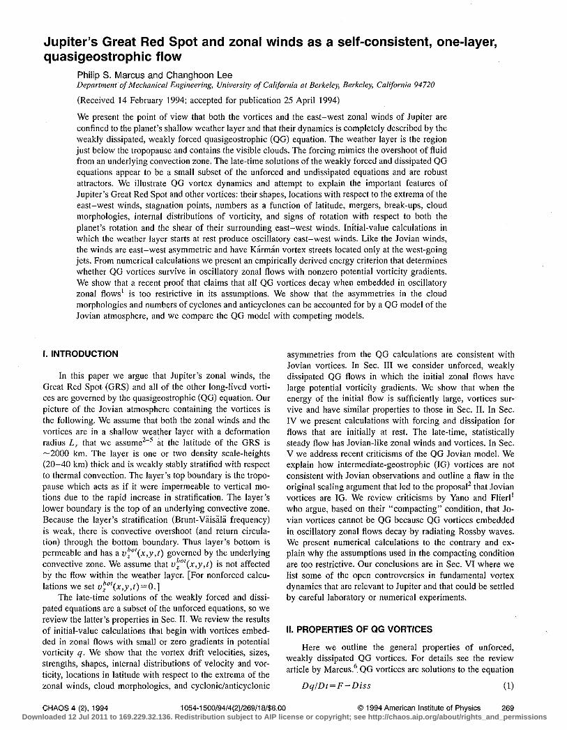
FIG. 3. The heavy curve from the origin to the + shows the relation between the energy E [following tradition (Ref. 16) an infinite constant is removed so that if the vortex were round-and not in general in equilibrium-the energy would be zero] and area A of the family of steady, stable, infinitc-L r , potential vortices with ij/uo= 1 embedded symmetrically in the cubic v of Eq. (9). The family ends with the limiting vortex at the +. The evolutionary paths of three different initiaJ vortices aTC shown as thin curves superposed with arrowheads placed at equal intervals in time. All of the vortices initially have elliptical boundaries and all arc attracted to the plus sign. The units of length and time are y* and (To]'

in an oscillatory v that is locally adverse. The figure is in the frame of reference where the center of the vortex is at rest, so v is approximately zero at the vortex center. If idqldyi is small, Eq. (8) is a good approximation, so an infinitesimal piece of q labeled A moves with v(r,l) "" v(r,I)+v(y). The Biot-Savart law gives v (shown with thin solid arrows); it is clockwise around the vortex, and at A vx = -qRy/2 (or less, if Ry"$>L,) where Ry is the vortex semiradius in y. Taylor expansion of v around the vortex center gives v; at A, v=Ryii. Thus if /iT/q/""O(1) (or less, if Ry"$>L,), fluid element A is dragged to the right and B to the left (shown with broken arrows). The clockwise motion of v then pushes A downward and out of the adverse zonal flow and into the adjoining prograde zonal flow. Similarly, B is pushed upwards into the northern prograde flow. If the sign of the shaded vortex were reversed so that it were prograde, then both v and v initially move A to the right and B to the left. Then the counterclockwise v would pull both A and B into the center of the prograde zonal flow. Thus for iT/q=O(l), prograde q is drawn in towards the center of a prograde zonal flow while adverse q is expelled. This effect has been confirmed by numerical calculations.3,6

All of the more than 100 Jovian vortices that have been identified are prograde with respect to the shear of V Lim'

Therefore the Jovian observations are consistent with QO. In contrast 10 calculations show that both prograde and adverse vortices can be long-lived2

A second argument for the persistence of prograde vortices is the numerical evidence that prograde QO vortices

merge together while adverse vortices do not. Thus if Jovian vortices are formed and maintained against dissipation by merging with smaller vortices (created by ageostrophic motions or by F) they should be prograde. The merger of prograde vortices has been explained using a simplified model of two uniform-q vortices embedded in a v. The merger of two prograde (adverse) vortices initially at the same or nearly the same latitudes decreases (increases) the energy of the flow. Therefore prograde mergers are energetically allowed and adverse mergers are prohibited.6,1l

D. Vortex size-large q / iT

A prograde vortex embedded in a v with a iT that changes sign as a function of latitude has stagnation points (as viewed in the frame where the vortex center is at rest) in regions where the zonal flow is adverse to the vortex. There are closed streamlines around the vortex, but the last closed streamline (LCS) is the one that passes through the stagnation point closest to the vortex. We now show that if ql iT is large at the vortex center, the location of the LCS determines the vortex size.

Using the simple model of a uniform-q vortex embedded in a quadratic or cubic zonal wind v also with uniform if, Van Buskirk and Marcus showed for infinite L ,. that if a vortex were to grow in area keeping its x-momentum (or mean latitude Yo) and value of q fixed, the area of the vortex A increases faster than the area circumscribed by the LCS.15 For sufficiently large A the vortex boundary coincides with the LCS. The latter vortex we define as the limiting vortex with finite area A lim' Families of steady or uniformly translating, stable vortices exist only for a <A ",A Ii",. Figure 3 shows with a heavy curve the energy E of the flow as a

40

30

'0

10

Y 0 0 -10

·'0

·30

-40

·40 -30 -20 -to 0 10 '0 30 40 .~

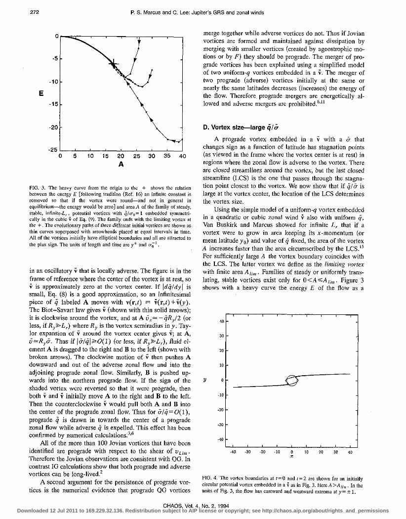
FIG. 4. The vortex boundaries at t=O and 1=2 are shown for an initially circular potential vortex embedded in a v as in Fig. 3. Here A >A lilll . In the units of Fig. 3, the flow has eastward and westward extrema at y = ± 1.


P. S. Marcus and C. Lee: Jupiter's GRS and zonal winds 273

function of A for the family of steady vortices with ij/uo=l, Yo=O, and embedded in the zonal flow

(9)

The curve starts at the origin and ends at the + in the figure which is the limiting vortex (not a turning point). Although the limiting vortex itself can be linearly unstable, all of the other vortices on the curve are linearly stable, because there are no turning points or other bifurcations on the heavy curve in Fig. 3.

Initial-value experiments show that as a vortex increases its area by merging with small vortices (with the same Yo and q as the original vortex) it progresses through a sequence of quasisteady states that correspond to the equilibria of the family. That is, an initially small vortex that is a steady solution has energy and A initially near the origin and lies on the heavy curve in Fig. 3. As the flow evolves it remains on the curve but moves to the right and ends at the +. Moreover, at all times its shape closely corresponds to an equilibrium vortex in the family. After the area of the vortex grows to A hm any subsequent area that is added to the boundary of the vortex circulates around the vortex until it reaches the stagnation point where it leaves the vortex, joins onto an open streamline, and is carried to infinity. Thus vortices that gradually increase their areas by mergers can overflow into regions where the east-west wind is adverse, but they have a natural limit to growth determined by the LCS.

Initial-value experiments using contour dynamics show a vortex, initially with A >A lilll , has its northern and southern extremities carried off to infinity primarily by V, and the flow never comes to a'steady state.6,15,17 See the example in Fig. 4. Dissipation can be added to this contour dynamics ca1cu-

3 t=O.O

2

(a) y ~ -1 -2 -3

-6 -4 -2 0 2 4 6

X

3 t=15.0

2 1

(c) YO -1 -2 -3

-6 -4 -2 0 2 4 6

X

lation by chopping off any part of the vortex tail that extends past Ixl=9.5. This mimics the actual dissipation of the tails when hyperviscosity or viscosity are used in spectral calculations. (For a discussion of the accuracy of this method, its insensitivity to the precise location where the tail is chopped, and a comparison with hyperviscosity see Van Buskirk and Marcus.!8) The evolutionary paths of three vortices each initially with A >A 1im and shown in Fig. 3 with thin lines and arrowheads are typical of a large number of simulations. The paths all go from right to left because the dissipation conserves ij and momentum, but decreases A monotonically. The energy can increase or decrease. All paths end near the limiting vortex. The slopes dE/dA of the evolutionary paths at late times (i.e., near the +) are equal to the slope of the heavy curve, which is dE/dA = -ij"'_"ag + (A h ,,,ij'/41f) In(Alimq/41f) where "'_<lag is the value of '" at the limiting vortex's stagnation point. The reason for equality is given by Van Buskirk and Marcus.6,!5 In general, the vortices relax to equilibrium by shedding all of the ij that lies outside the

instantaneous LCS via the vortex tails that extend outward from the stagnation points. The area circumscribed by the vortex boundary decreases until the boundary lies just inside the LCS. (See Fig. 5.) This occurs near the limiting vortex. Thus both for small vortices that grow in size by merging with other vortices (n.b,; the other vortices can be created as in Sec. IV by an appropriate F) and for big vortices that are larger than A lim' the equilibria in the neighborhood of the limiting vortex are robust attractors (and are therefore nonlinearly stable). For these vortices the final size is determined by the stagnation points of the limiting vortex. Analytic approximations of the limiting vortices, in good agreement

3 2

Y~ (b)

-1 -2 -3

-6 -4 -2 0 2 4 6

X

3 2

Y~ -1 (d)

-2 -3

-6 -4 -2 0 2 4 6

X

FIG. 5. The lime evolution of the boundary of an initially circular vortex embedded in the cubic v of Eq. (9). This vortex corresponding to the middle evolutionary path in Fig. 3 with initial A = 30. Paris (a) and (b) arc computed with no dissipation, but (c) and (d) have the dissipation described in Sec. II. For lyl>l, ir is adverse.



with numerical calculations, including their sizes and shapes have been determined. 15

In the limit y* .... ~oo it has been shown l5 that the heavy curve of equilibria in Fig. 3 becomes the Moore-Saffman family llJ of steady elliptical vortices. In the same limit other

families of linearly stable vortices exist such as the oscillating Kida ellipses, and we presume that there are analogs of those families for finite y*. However, we have not been able to find initial conditions relevant to Jupiter that evolve to Kida-Iike vortices. The contrived initial conditions that do evolve to vortices that oscillate do so with amplitudes less than a few degrees, so they are nearly the same as the steady vortices. [S In the limit y*~oo, we find that when we initialize the flow with a linearly stable oscillating Kida vortex it is quickly destroyed when we let it interact with other vortices. One of the main points of this paper is that although there can be several linearly stable solutions to the inviscid equations, the only ones that are relev~nt to the turbulent Jovian flow at late times are those that are robust attractors.

Contour dynamics calculations show that as L,. is decreased the heavy curve in Fig. 3 develops a turning point near the +, so the branch between the limiting vortex and the turning point becomes linearly unstable. When a small vortex with finite Lr grows by mergers, it only increaSes in size until it reaches its turning point. Although the boundary of the attracting vortex extends into the region of adverse shear, it does not reach the stagnation point. These families of vortices are called corner-like because their infinite-L ,. counterparts have corners at the stagnation points on their boundaries. Consistent with these QG vortices, many Jovian vortices overflow their local prograde ij and extend into regions of adverse shear almost to the stagnation points. A

quantitative comparison between Jovian vortices and QG vortices at the turning points is not possible because of the uncertainties of the data. Moreover, many Jovian vortices have one or two of their extremities lying in zonal flows with large values of prograde shear for which the proceeding analysis does not apply. We now consider the robust attractors associated with these vortices.

E. Vortex size-small ijl u When q is uniform an element of q on a vortex bound

ary is advected by u(y)x+ v. For finite-L,. QG vortices, v has exponentially small effect over distances greater than L /"' so for vortices embedded in zonal winds with large ir the exponential screening effects of L r are too strong for the vortex's v to have much influence on its northern and southernmost extremities. The extremities are stretched in x by v with the result that as a family of steady-state vortices increases its A, the additional area is not added equally to all parts of the vortex but preferentially to its eastern and western ends. As A increases, the vortex goes from a nearly eiIiptical shape (exactly elliptical with the ellipticity given by the Moore-Saffman relation for a uniform-q vortex with A ->0, regardless of the value of L,) to a much more elongated band-like shape. Asymptotically the growth on the northern and southern sides stops while the vortex continues to expand in longitude. A family of uniform-q vortices asymptotes to an east-west band of q bound between two fixed

values of latitude, with half-height Ymax , and extending to x= ±';I). These families of vortices are distinct from cornerlike families because their equilibrium curves of energy as a function of A (cf. Fig. 3) do not have limiting vortices, or turning points. They extend to A ->00. For the simple case of uniform-q vortices embedded symmetrically in the cubic v of Eq. (9), we have derived the analytic approximation: Vortices are band-like if

(10)

otherwise they are corner-like.6,2() Contour dynamics confirm

the approxim.ation is accurate for uniform-q vortices, and spectral calculations of nonuniform-q vortices embedded in V without uniform q show similar behavior. Initial-value experiments where Eq. (10) is satisfied show that as a vortex increases its A by mergers, it grows flatter. Its northern and southern boundaries never reach the region of adverse ir. The band-like vortices that we have found numerically are ail lif!early stable. in inc iimit y* /Lr-)w, an analytic approximation for the asymptotic half-height Ymax of band-like vortices is

y """ = L ,.( 3q I 4 (To) 1/3. (11)

Equation (11) has been confirmed by contour dynamics, and is a good approximation for finite values of y *. Equation (11) shows that for a wide range of iflq, the half-height Yrnax is order L r . Several Jovian vortices, especially the cyclonic barges at 14 ON and the three very elongated cyclones at 300 S look band-like. Like all families of band-like vortices the cyclonic Jovian barges increase their eccentricity with increasing A .

In the limit A --tOO the band-like family of prograde vortices described by Eq. (11) is a special case of the larger family of equilibrium uniform-q vortex layers with boundaries that are two lines of constant latitude separated by

2 Y """ [with Y m" in these families not constrained by Eq. (11)]. A prograde vortex layer is linearly stable 17 if uulq>c-2YIll<lxIL'(LrIY maX>, so for O"olq>O.l the vortex layers that are the infinite area limits of band-like vortices [i.e., with Y m", given by Eq. (11)] are linearly stable. These vortex layers are also nonlinearly stable robust attractors. Numerical calculations show that as finite-A, band-like vortices are weakly forced (by introducing small vortices into the flow) and dissipated with hyperviscosity (which allows mergers), they grow and are attracted to the one-parameter family of vortex layers given by (11). Therefore as in the case of corner-like vortices, forcing a~d dissipation lead to robust attractors.

Because of the screening effects of L ,., it should be no surprise that the north and south sides of a vortex can act independently of each other. An asymmetric vortex can have a northern boundary that acts cQrner-like and extends into the region of adverse shear and a southern boundary in large prograde if that acts band-like. No matter how large A becomes the vortex is bounded to the south in prograde shear. We argue in the next section that many Jovian vortices lie asymmetrically in their local v and are hybrids of corner-like and band-like vortices.

CHAOS. Vol. 4. No.2. 1994 Downloaded 12 Jul 2011 to 169.229.32.136. Redistribution subject to AIP license or copyright; see http://chaos.aip.org/about/rights_and_permissions


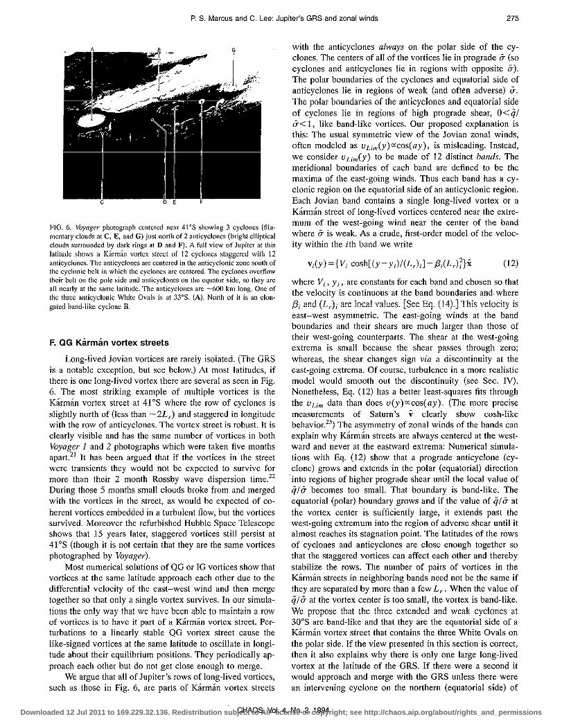
FIG. 6. Voyager photograph centered ncar 41 oS showing 3 cyclones (filamentary clouds at C, E, and G) just north of 2 anticyclones (bright elliptical clouds surrounded by dark rings at D and F). A full view of Jupiter at this latitude shows a Karman vortex strcct of 12 cycloncs staggered with 12 anticyclones. The anticyclones arc ccntered in the anticyclonic zonc south of the cyclonic belt in which the cyclones arc centered. The cyclones overflow their belt on the pole side and anticyclones on the equator side, so they ,IfC

all nearly at the same latitude. The anticyclones arc -600 km long. One of the three anticyclonic White Ovals is at 33°S. (A). North of it is an ciongalea band-iike cydone B.

F. QG Karman vortex streets

Long-iived jovian vortices are rareiy isoiated. (The GRS is a notable exception, but see below.) At most latitudes, if there is one long-lived vortex there are several as seen in Fig. 6. The most striking example of multiple vortices is the Karman vortex street at 41°S where the row of cyclones is slightly north of (less than -2L,.) and staggered in longitude with the row of anticyclones. The vortex street is robust. It is clearly visible and has the same number of vortices in both Voyager 1 and 2 photographs which were taken five months apart." It has been argued that if the vortices in the street were transients they would not be expected to survive for more than their 2 month Rossby wave dispersion time.22

During those 5 months small clouds broke from and merged with the vortices in the street, as would be expected of coherent vortices embedded in a turbulent flow, but the vortices survived. Moreover the refurbished Hubble Space Telescope shows that 15 years later, staggered vortices still persist at 41°S (though it is not certain that they are the same vortices photographed by Voyager).

Most numerical solutions of QG or IG vortices show that vortices at the same latitude approach each other due to the differential velocity of the east-west wind and then merge together so that only a single vortex survives. In our simula-tions the only way that we have been able to maintain a row of vortices is to have it part of a Karman vortex street. Perturbations to a linearly stable QG vortex street cause the like-signed vortices at the same latitude to oscillate in longitude about their equilibrium positions. They periodically approach each other but do not get close enough to merge.

We argue that all of Jupiter's rows of long-lived vortices, such as those in Fig. 6, are parts of Karman vortex streets

with the anticyclones a/ways on the polar side of the cyclones. The centers of all of the vortices lie in prograde ir (so cyclones and anticyclones lie in regions with opposite ir). The polar boundaries of the cyclones and equatorial side of anticyclones lie in regions of weak (and often adverse) ir. The polar boundaries of the anticyclones and equatorial side of cyclones lie in regions of high prograde shear, O<ql 0-< 1, like band-like vortices. Our proposed explanation is this: The usual symmetric view of the Jovian zonal winds, often modeled as v,.;",(y)o:cos(ay), is misleading. Instead, we consider vu",(y) to be made of 12 distinct bands. The meridional boundaries of each band are defined to be the maxima of the east-going winds. Thus each band has a cyclonic region on the equatorial side of an anticyclonic region. Each Jovian band contains a single long-lived vortex or a Karman street of long-lived vortices centered near the extremum of the west-going wind near the center of the band where ir is weak. As a crude, first-order model of the velocity within the ith band we write

v;(y)={V; cosh[(y-y;)/(L");)-.B;(L,)f}x (12)

where Vi' Y i, are constants for each band and chosen so that the velocity is continuous at the band boundaries and where f3i and (Lr)i are local values. [See Eq. (14).J This velocity is east-west asymmetric. The east-going winds at the band boundaries and their shears are much larger than those of their west-going counterparts. The shear at the west-going extrema is small because the shear passes through zero; whereas, the shear changes sign via a discontinuity at the east-going extrema. Of course, turbulence in a more realistic model would smooth out the discontinuity (see Sec. IV). Nonetheless, Eq. (12) has a better least-squares fits through the vu", data than does v(y)o:cos(ay). (The more precise measurements of Saturn's v clearly show cosh-like behavior."3) The asymmetry of zonal winds of the bands can explain why Karman streets are always centered at the westward and never at the eastward extrema: Numerical simulations with Eq. (12) show that a prograde anticyclone (cyclone) grows and extends in the polar (equatorial) direction into regions of higher prograde shear until the local value of iii ir becomes too small. That boundary is band-like. The equatorial (polar) boundary grows and if the value of iii ir at the vortex center is sufficiently iarge, it extends past the west-going extremum into the region of adverse shear until it almost reaches its stagnation point. The latitudes of the rows of cyclones and anticyclones are close enough together so that the staggered vortices can affect each other and thereby stabilize the rows. The number of pairs of vortices in the Karman streets in neighboring bands need not be the same if they are separated by more than a few L,. When the value of iii ir at the vortex center is too small, the vortex is band-like. "·/e propose that the three extended and \veak cyclones at 300 S are band-like and that they are the equatorial side of a Karman vortex street that contains the three White Ovals on the polar side. If the view presented in this section is correct, then it also explains why there is only one large long-lived vortex at the latitude of the ORS. If there were a second it would approach and merge with the GRS unless there were an intervening cyclone on the northern (equatorial side) of



the GRS. However, there are no long-lived vortices in the zonal wind north of the GRS because that region is close to the equator where 10 is small, and the flow is threedimensional and turbulent. There is a row of like-signed vortices in Jupiter's northern hemisphere that does not appear to be part of a Karman street, but those vortices constantly merge with each other, and new vortices continually form to replace those that are swallowed.

Note that the model v Um in Eq. (12) with <t/>o' = 0 implies that each band has uniform q, and that ij is a monotonic step-function decreasing from north to south. In Sec. 1II we show that similar zonal winds (without exactly uniform q and without discontinuities) have very robust vortex streets. Moreover, numerical simulations with dissipation, forcing, and no initial velocity produce v similar to Eq. (12) and a Karman vortex street. (See Sec. IV.)

G. Cyclonic/anticyclonic asymmetry in QG vortices

The QG equation (1) with F=Diss=O and <t/'OI(y) = ifJ'''''( - y) is invariant under (x,y, ifJ) ~ (x, - y, - ifJ) so one expects cyclones and anticyclones to behave similarly. On Jupiter they appear not to; their associated cloud morphologies are different, and anticyclones are generally stronger and more prevalent than cyclones. These facts have been used to argue that the Jovian atmosphere inust therefore be IG or governed by another dynamical system that breaks cyclonic/anticyclonic degeneracy. Here we argue that the observations are in fact consistent with QG.

Figure 6 shows that the clouds associated with anticyclones are smooth, and nearly elliptical clouds, while those with cyclones are often filamentary and twisted (especially in the southern hemisphere). Our point is that the tracers that make up the clouds and ifJ are not necessarily aligned. Dissipation in the weather layer can create a weak Ekman-like circulation even when there are no solid boundaries. The predicted vertical velocities are too weak to detect directly, but Flaser et al24 used infrared measurements from Voyager to deduce that in the upper part of the GRS and the cyclonic barges there is up-welling where w/fo<O and down-welling where w/Io > O. A simulation of the Jovian clouds was carried out by assuming that the visible vapor in the clouds advects with. the horizontal v and that it is created randomly in small cloudlets where the flow is cooled by up-welling in the subadiabatic weather layer and destroyed where it is warmed by down-welling. 25 Thus cloudlets were created inside the anticyclones and just outside the boundaries of the cyclones, and they were randomly destroyed inside the cyclones and just outside the anticyclones. The velocities of the cyclones and anticyclones were computed with QG codes and included both coherent vortices and smaller scale turbulence. Clouds like those in Fig. 6 were created. Tracers filled the interiors of the anticyclones where the differential rotation and turbulence homogenized them. Tracers pushed outside the anticyclones were destroyed and left a circumferential ring with a tracer density lower than the ambient background (like the dark rings around the anticyclones in Fig. 6). Cloudlets created outside cyclones were repeatedly sheared by v and twisted by the turbulence. These tracers never homogenized. Thus the cyclonic/anticyclonic asymme-

try of the clouds can be due to the asymmetry in the location of the tracers' birth and death rather than the flow dynamics.

Not all parameters give cloud patterns that look like Fig. 6. To reproduce the pattern of vortex street at 41°S requires that the street's cyclones are weaker than its anticyclones. In general, Jovian cyclones (especially in the southern hemisphere) are weaker than anticyclones, cf. the elongated cyclones at 300 S compared with the anticyclonic GRS to the north and the three White Ovals to the south. When calculations include a forcing F that models the overshoot from an underlying convective layer, the maxima of F are greater in absolute value than its minima. Preliminary calculations show that this creates weaker and fewer cyclones than anticyclones, but those calculations are outside the scope of this paper.

More than 90% of the Jovian "spots" cataloged by Mac Low and Ingerso1I26 were anticyclones, but this statement can be misconstrued. They saw many vortex births, deaths, and mergers during their 58 days of observation, and the merger of vortices at the same latitude was very common if the vortices were not part of a Karman vortex street, so many of the vortices are short-lived. Moreover, Mac Low and Ingersoll classified a vortex as a "spot" or a "filamentary region." The latter was defined as "a turbulent cyclonic region containing many shifting strands of light clouds." Thus all of the cyclones labeled as filamentary regions were excluded from the census that led to the 90% figure.

We argue both from theory and our informal observations of the Voyager photographs and movies that with the exception of the vortices near the equator, long-lived Jovian vortices are parts of Karman streets, and we conclude that there are approximately equal numbers of long-lived cyclones and anticyclones. The asymmetry in number applies. only to the ephemeral vortices that decay or merge and whose existence, we surmise, is due to F.

III. VORTICES IN ZONAL FLOWS WITH dq(y,t)/dy* 0

For flows with uniform ii(y, t = 0) and initial prograde vortices with internal distributions of ij(X,I= 0) that decrease monotonically outward from the vortex center, we find that the vortices are robust. They adjust their shapes and often shed ii, but they survive. Vortices with nonmonotonically decreasing liil are also robust for finite L" and can have large outwardly increasing gradients of Iql near their centers. Recently, I questions have been raised whether these numerical experiments were atypical because Rossby waves are prohibited when dij(y,t)/dy=O. Although, none of the numerical experiments described in the previous section (that were carried out with spectral methods) have dq(y,t)/dy=O at late times (due to the mixing of q from the initial flow), it is useful to show that the results summarized in Sec. II are still true when dq(y,I=O)/dy*O.

Consider flow on a f3 plane in a doubly periodic computational box of size LxXLy . The [q(y ,I) - f3y 1 is periodic in y. We choose

- [tanh(Y/~) 1 q(y,I=0)=0.5f3L y (1 + Y)tanh(Ly/2~) - y2y/Ly (13)

CHAOS. Vol. 4, No.2, 1994 Downloaded 12 Jul 2011 to 169.229.32.136. Redistribution subject to AIP license or copyright; see http://chaos.aip.org/about/rights_and_permissions


for -L)J2""y<L)J2. For 1'=0 and D.!Ly-->O. ij(y. 1=0) ·is a step-function with jumps in ij of (3L y at integer values of y/Ly. and

- jcoSh[(Y-Ly/2)IL,] 1 v(y.I=O)=O.S(3L yL,. <;nh(T I?T \ -2L,.fL y

l .,. .... \~yl ~~r' ) (14)

for O~y~L)'. We have found that all of our numerical experiments. with the exception of those flows where v(x,I=O)=O and ii(y,I=O) is linearly stable, blow up if there is no hyperviscosity or some other form of small-scale dissipation. Our hyperviscosity, which is an extension of the Smagorinsky dissipation, is included by setting Diss in Eq. (I) to

Diss=(Cj2EN/k 12 )V I2 W(X t) mnx , (IS)

where C is a dimensionless constant of order unity (5 in this paper, and chosen to minimize rapid changes in the energy spectra at small scales), EN = f w 2dA!2L,L, is the average enstrophy density, and km;O( is the maximum wave number. The dissipation conserves potential circulation and momentum and dissipates small-scale energy and enstrophy. The order of the V operator in (IS) was chosen by experimentation. It is the optima! in the sense that with V 12 the numerical solutions computed with different values of spatial resolution alI have nearly the same large-scale flows, yet the decay rate of enstrophy remains low. In addition, with V 12 the value of C was nearly independent of the resolution for a wide variety of flows. The maximum resoiution used in the cakuiations in Secs. III and IV is S 12 X S12.

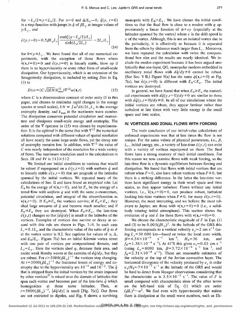
We limited our initial conditions to vortices that would be robust if superposed on a ii (y ,I = 0) with uniform ij and to linearly stable ii (y, t = 0) that are prograde at the latitudes spanned by the initial vortices. We repeated many of the calculations of Sec. " and have found an empirical rule: Let Eo be the energy of v(x,I=O), and let E" be the energy of a zonal flow with uniform q and with the same x-momentum, potential circulation, and integral of the streamfunction as v(x,t=O). If Eo";3EI/ the vortices survive; if Eo<EI/; they shed large amounts of ij and become much smaller; and if Eo""E" they are destroyed. When Eo~E", the late-time ii(y,t) changes so that Idij/dYI is small at the latitudes of the vortices. Exampies of vortices that survive or decay in accord with this rule are shown in Figs. 7-9. In each casc L,.= O.IL y and the characteristic value of the ratio of ij to (j at the vortex center is 0.2. See captions for values of y, 6., and Eo/E". Figure 7(a) has an initial Karman vortex street with one pair of vortices per computational domain, and Lx = L y' Here the vortices shed q, decrease their area, and excite weak Rossby waves at the extrema of dij/dy, but they are robust. For t> SOOO((3L y) -I the vortices stop changing. il..t t=5000(j3L y )-1 the fractional losses of energy and enstrophy due to the hyperviscosity are 10 - 5 and 10 - 2. The q that is stripped from the initial vortices by the strain imposed by other vortices27 is mixed over the domain of latitudes that span each vortex and becomes part of the late-time ij which homogenizes at those same latitudes. Thus, at t=SOOO((3L y)-I, Idij/dYI is small [Fig. 7(c)]. Our flows are not restricted to dipoles, and Fig. 8 shows a surviving

monopole with Eo>EI/' We have chosen the initial conditions so that the final flow is close to a modon with q approximately a linear function of ifl+cy (especially at the latitudes spanned by the vortex) where c is the drift speed in x of the vortex. Although, this is not an isolated vortex due to the periodicity, it is effectively so because it is separated from the others by distances much larger than L r' Moreover, we have repeated the calculation with twice the computational box size and the results arc nearly identical. We include the modon experiment because it has been argued analytically that one-layer, QG, monopolar modons embedded in oscillatory zonal flows with dij/dy",O cannot be robust. (See Sec. V B.) Figure 9(a) has the same ij(X,I=O) as Fig. 7(a), but u(y,t=O) is different with Eo<E". The initial vortices are destroyed.

In general, we have found that when Eo";3EI/ the numerical experiments with dij(y,1 = O)/dy '" 0 are similar to those with dij(y,t=O)/dy=O. In all of our simulations where the initial vortices are robust, they appear laminar rather than turbuient at iate times with very iWie energy in the smaii space and time scales. '

IV. VORTICES AND ZONAL FLOWS WITH FORCING

The main conclusion of our initial-value calculations of unforced experiments was that at late times the flow is not unique. For the same values of physical parameters, i.e., /3, L r , initial energy, etc., a variety of late-time v(y,t) can exist with a variety of vortices superposcd on them. The final flows have a strong memory of their initiai conditions. For this reason we now examine flows with weak forcing, so the late-time flow is a dynamic equilibrium between forcing and dissipation. We found that flows with initial vortices that are robust when F=O, also have robust vortices when F=f::.O, but there is a striking difference. In the latter the latc-time vortices have significant energy in their small space and time scales, so they appear turbulent. Flows without any initial vortices, Le., v(x,t=O)=O, can produce robust, turbulent looking late-time vortices when F", 0, for many ii (y, 1 = 0). However, the most interesting, and we believe the most relevant to Jupiter, are those with V(X,I=O)=O (i.e., a solidbody rotating initial atmosphere). This section shows the evolution of q and ii for three flows with v(x,I=O)=O.

We choose the characteristic magnitude of F in Eqs. (l) and (3) to be O.OOS((3L y)'. At the latitude of the GRS this forcing corresponds to a vertical velocity uz=2'cm S-l (using L y =30 000 km-based on twice the local zone width, (3=4.S4XIO- 9 S-I km-I, Ho=30 km, and 10= 1.38X 10- 4 S-I). At 41'S this gives v,=O.OS cm S-I (using L y =8000 km, (3=3.72X 10-9 S-I km-', and 111= 2.31 X 10 - 4 S - I). These are reasonable estimates of the velocity at the top of the Jovian convective layer. The horizontal divergence of the velocity produced by v z is order v,/Ho=7X 10- 7 S-I at the latitude of the GRS and would be hard to detect from Voyager observations considering that the characteristic w is 3.SX 10-5 S-I. The value of F is small compared with characteristic sizes of the other terms on the ieft-hand side of Eq. (I) which are order ((3L )2_ w 2 We find even with hyperviscosity that unless there is dissipation at the small wave numbers, such as Ek-



(a) (b)

0.8 ~-""" ............... , .......

0.8

0.6 0.6

(c) Y 0.4 0.4

(d)

0.2 0.2 ".,.,"'"

".

0 0 ·0.4 ·0.2 0 0.2 0.4 ·0.02 ·0.01 0 0.01 11.02 !I.lll

q(y) v(y)

FIG. 7. The qat (=0 (a) and at latc-time t=5000 (b) as functions of x and y. Time and length in Figs. 7-12 are in units of (f3L y )-1 and Ly . The initial ij has y= - 0.7 and 6. = 0.15. The initial v has EoIEI/= 1.57. The two initial vortices, which arc 7:9 ellipses, have maximum and minimum strengths of q(x,t=O)= ±O.3. Here, the blackest and whitest pixels arc q= :to.S. To break symmetry noise is added to the initial q in Figs. 7-12 with amplitude 10-3, The initial and 1=5000 q(Y,t) and ii(y,t) arc shown as dotted and solid curves in (c) and (d).

man pumping, the strengths of the vortices grow indefinitely. With some types of forcing the net late-time growth is very small because the flow adjusts itself so that net effects of F cancel. For example, with rectangular forcing with wave number p,

F=A «(3Ly)2 sin(2pTrx/Lxl sin(2pTry/L y ) (16)

the vortices drift in x, so the net influence of F on a vortex averages to nearly zero. For rectangular forcing the late-time growth rate of the vortices is -10-4(3Ly ' When an Ekman dissipation of the form

Diss= W(3LylT (17)

is included in Eq. (1) with T';;; 104 the vortices come to a dynamic equilibrium such that the vortex strength asymptotes to a value that depends on 'T.

Figure 10 shows the flow with rectangular forcing as in Eq. (16) with p=2, A =0.003, -r=30 000 and L r =O.lL y . Weak variations in q with spatial scales of order the forcing length quickly appear, but in no sense is there any spatial or temporal coherence in the flow, and fluctuations in ij of both signs appear and disappear at approximately random locations. However the characteristic strength of these early-time fluctuations is nearly equal to strengths of the coherent vortices which appear after t>'3000«(3L y)-I. They have strengths -«(3L y ) and last five to ten turnarounds times before filamenting or merging. At about this same time, the mean zonal flows begin to develop. The y wavelength of the flow is Ly (but can be a subharmonic of Ly for other forcing parameters). At t>4000«(3L y)-I, v(y,t) starts to show signs of homogenization28 of ij(y,t) with two distinct re-



(a) (b)

(e) (d) (e)

0.8

0.8 0.8 0.6

0.4 0.6 0.6

0.2 Y Y q

0.4 0.4

-0.2

0.2 0.2 -0.4

-0.6

0 0 -0.8 ·0.4 -0.2 0 0.2 0.4 -0.02 -0.01 0 0.01 0.02 0.03 -1 -0.8 ·0.6 -0.4 -0.2 0 0.2

q(y) v(y) H,' L,

FIG. 8. Same as Fig. 7, but the q(x,t=O) less than zero is sella zero so Ihe flow is a monopole. Here EnIE,,= 1.52, and the late-time flow (b) is shown at t=4000. The late-lime flow is well-approximated by a modon as shown in (c) by the relation between q and ifi·

gions: q=(?-0.5)[3Ly for O<y/Ly<? and ij=(?+0.5)[3Ly for ?<y/Ly<1 with O<?<1, and with the value of ? a function of the forcing and initial noise. Figures lO(e) and 10(g) show that the degree of homogenization is a sensitive function of A. The forcings in this section approximately conserve the initial potential circulation. The v(y ,1) approaches Eq. (14) with a shift in y corresponding to the value of r At late times the I o-(y, t) I of the flow in Fig. 10 is order 0.15([3L y)-I. After the v(y,t) becomes established, the potential vortices embedded within it change character. They segregate location in y so the vortices are prograde with respect to v. Vortices of like sign merge, so that at late times there is one dipole vortex pair per computational wavelength Lx (Le., Jovian circumference), but for different parameters of forcing, dissipation, and L, there could be more than one pair. The characteristic strengths at late time of 0- and the q of the vortices depend strongly on the values of A and weakly on r.

Zonal forcing is another way of producing vortices and is similar to the one in the laboratory experiments of Sommeria et al. 29 We choose a Gaussian zonal forcing

F=A ([3Ly)2 (e-ty-Yo)2/D2 -e-tY+Yo)'/D'). (18)

Figure 11 shows the flow with A=0.005, D=0.03, Yo=Ly/4, L,=0.1Ly , and r=100. Because of the geom-

etry of the forcing, drifting vortices do not time-average the forcing to zero, so a small value of r= 1 00 (in the laboratory experiments r-1 0) is needed and the late-time vortices look relatively laminar. By 1=400, the flow forms several vortices at the latitudes of the extrema of the forcing with the sign of q the same as the local value of F. The vortices begin to merge together at about the same time that v forms and shows homogenization of q. Typically, we find that the homogenization increases with decreasing D and strongly depends on 7, though in general it is not as good as with rectangular forcing. At late times there is one dipole vortex pair per computational wavelength Lx, but for different values of A, D, 7, and L r there are more.

At late times 10-(y,t)I-O.15([3Ly)-1 and Iq(x,t)I-0.5([3L y) -I for the vortices. All of the vortices in this section have small values of Iwl at the vortex center with I wi maximum at the vortex edges. However, the late-time vortices in Fig. 11 have a slightly smaller value of I ij I at the vortex center as does the GRS (see Sec. II B). Also note that the late-time vortices are slightly east-west asymmetric.

Figure 12 shows a flow with temporally pulsed/spatially rectangular forcing. The forcing is defined as in Eq. (16) with p=4, r=20 000, and A=0.003a2:~"oo(t-ia), with a= 40([3Ly) -I. The flow is similar to the steady rectangularly forced p = 2 flow in Fig. 10. However, at late-times the

CHAOS, Vol. 4, No.2, 1994

Downloaded 12 Jul 2011 to 169.229.32.136. Redistribution subject to AIP license or copyright; see http://chaos.aip.org/about/rights_and_permissions


(a) (b)

FIG. 9. Flow with the same q(x,1 = 0) as Fig. 7, but the initial q has y= 0.3 and 6. = 0.15, and the initial v has 'Eo/E" = 0.49. The q is shown at t= 0, 100, 400,4000, and q(y) and u(y) arc at 1=4000.

10-1 and l<il are slightly larger, and the homogenization of <i is slightly better.

The purpose of this section was not to present an exhaustive study of parameters, but to show that both vortices and zonal flows can be made from an atmosphere initially at rest with forcings that mimic convective overshoot from a lower layer. We should note that for a large region of parameter space coherent zonal flows do not form, but when they do, the values of their average shears and the strengths of the vortices are sensitive functions of parameters. We also note that when the forcing is cyclonic/anticyclonic asymmetric (i.e., the minima and maxima of F have different absolute values) the flow can produce a single coherent monopolar vortex rather than dipoles.

V. CRITICISMS OF THE QG MODEL

Here we address three recent criticisms of our QG model of the Jovian weather layer.

A.IG models

Williams and Yamagata2 rejected OG theory for Jovian vortices because they believed the required scalings were

incorrect. The approximations needed for OG theory are the usual shallow-water approximations plus the additional scalings: I",E ~ [v]/l/ol[l]~[w]/l/ol, o,8[Y]/l/ol, E~[I/I]/l/oIL; and E ~ [iftbOl]ll/oIL;, where [y] is the characteristic meridional extent of the vortex, [I] is the characteristic length of the vortex, and [v], [w], and [ift] are the characteristic values of their respective quantities. Calculating wand 1/1 by differentiating and integrating the Voyager v shows that the Jovian vortices are consistent with OG scalings (assuming reasonable values of [1/1>01]). Williams' analysis did not use the Voyager v. He estimated the value of [1/1] from [ift]~[w][1]2, so for a flow to be OG he required ([I]IL,/"'; 1. Using L,.~ 2000 km and [I] ~ 17000 km, the latter being the average radius of the GRS, gives ([I]IL,)2",1, and [ift]~[w](17 000 km)'. From this Williams argued that Jovian vortices are either planetary geostrophic or !G, but not QG. However, we argue that [I] should be the characteristic distance over which 1/1 and v change (which is order L,) not the size of the vortex. Thus we argue [ ift] ~ [w]L,' which is consistent with the calculations from the Voyager data. Williams has overestimated the value of [1/1]. The reason that [ift]~[w]L;, is that [ ift- I/Iu",(Y)] is a top-hat function: nearly constant outside



(e) (9)

/ /

0.8 / 0.8 0.8

/

/ /

/ /

0.6 / 0.6 0.6

Y /

/ Y Y

OA / OA 0.4

/ /

/ / 0.2 0.2 0.2

/ / /

" U ·(Ui u.~ U.2 U u.2 U.' U.1i ·0.U2 -0.01 0 0.01 0.02 0.03 -0.6 -0.4 -0.2 0 0.2 OA 0.6

q(y) v(y) q(y)

FIG. 10. Flow starting at rest (a) with rectangular forcing with amplitude A =0.003. The blackest and whitest pixels have q=::t 1. As shown in (a) the extreme values at (=0 arc :t:O.S. The I in (b), (c), and (d) arc 1600, 3000, and 5000. The 1=0 and 1=5000 q(y) and u(y) arc shown as dashed and solid curves. As a comparison (g) is the late-lime q(y) for rectangular forcing withA=O.004.

and inside the GRS with the latter value much smaller. The value of [!f!- !f!u",(Y)] only changes appreciably in the highspeed circumferential ring at the outer edge of the GRS which has a width of order L r .

We have already noted that the planetary-geostrophic and IG models of the GRS have w Gaussianly peaked at the vortex center, and there is no high-speed circumferential flow at the edge of vortex. This is in direct contradiction with the observations of the GRS and with the predictions of QG theory. We have also noted that the Jovian vortex drift speeds are not consistent with IG theory.

Our other concerns with the IG model is that in numerical simulations of IG vortices Williams found in order to maintain multiple IG vortices at the same latitude there must be a delicate balance so that they all move at the same speed (otherwise one catches up with another and they merges). It would be hard to maintain that long-term balance in the turbulent Jovian atmosphere.

B. Deep layer models

Yano and Flierl' state that the one-layer QG equation with an oscillatory zonal flow (Le., the equation and v examined in this paper) does not allow isolated vortices be-

cause they decay by Rossby radiation. Here we examine their proof and discuss our numerically computed counterexamples.

Restricting their analysis to the one-layer equation (1) with F=Diss=O, their arguments simplify: Assume that in a frame moving in x with speed c the flow is steady, so Eq. (1) reduces to q=q(!f!+cy). Now make the more restrictive assumption that the flow is a modon of the form q = a(!f! + cy) + b where a and bare co_nstants. If the vortex is compact in space, then far from it !f! must be small, so

q(y)=a[ ",(y)+cy] + b. (19)

Equations (1), (2), (19), and the modon assumption imply

\I''''(X,f) = (a +L;2) "'. (20)

Finally, assume that ",(y) is sinusoidal with wavelength I. This last assumption is consistent with Eqs. (1), (2), and (19) if and only if ¢l01 is linear in y and/or sinusoidal in y. Yano and Flier! consider the linear case which requires (a+L;2)= -(2"'/£)'. Using this in Eq. (20) implies

\I''''(x,t)= -(2",/1)2",. (21)

Yano and Flier! argue that for a vortex to be compact, !f! must have a positive eigenvalue of \1 2 (i.e., '" decays exponen-



(a) (b) (c)

(d) (e) (f)

I I

0.8 0.8

0.6 0.'

Y Y

0.4 0.4

I I

0.2 u.2 I

I

U 0 -0.6 -0.4 -0.2 0 0.2 U.4 0.6 -0.015 -0.01 -0.005 0 0.005 0.01 0.015

q(y) v(y)

FIG. 11. Flow starting at rest (a) with Gaussian zonal forcing. The blackest and whitest values of q arc :':0.5 including (a), The t in (b), (c), and (d) arc 500, 900, and 2000. The t=O and t=2000 q(y) and u(y) arc shown as dashed and solid curves.

tially far from the. vortex). Because the ;p in Eq. (21) violates the compactness condition, they argue that an initially compact vortex will decay by (sinusoidal) Rossby radiation. Their more general two-layer analysis shows that vortices satisfy their compactness condition only if the deformation radius associated with the zonal component of the flow L, is greater than that associated with the vortices i r from which they conclude that the zonal flow of Jupiter must be very deep Cseveral thousand kilometers or several hundred density scale-heights) while the vortices must be shallow and very baroclinic. In the limit that L, is large, they find that compactness requires I> 2 7I"L, from which they conclude that vortices have IG rather than QG scaling (see Sec. V A).

In apparent contrast to the analysis above, we have carried out many numerical calculations with oscillatory ii (y) where isolated, one-Iaye'r QG vortices survive. The calculations in Sec. III have dij/dY"FO, so ii(y) supports Rossby waves. We surmise that the numerical vortices of Yano and Flier! decay because their initial conditions have Eu>Eo. To reconcile our numerical results with their analytic proof, consider the robust vortex in Fig. 8 which approximately satisfies their modon assumption. The analysis of Yano and Flier! is only local, and in Fig. 8 the oscillatory ii (y) acts locally

like a cosh rather than a cos. Therefore the value of 1 i~ Eq. (21) is imaginary, the eigenvalue is positive, and the I/J far from the vortex has exponentially decreasing rather than sinusoidal behavior Cas confirmed by the numerical values). Thus we argue that the proof's assumption that ii (y) is sinusoidal is too restrictive. It precludes the important case of vortices embedded in flows where locally dij/dy is small but not zero [which implies locally cosh-like behavior in ii(y)]. We remind the reader that our original two arguments that the Jovian ii(y) at the latitudes of the vortices is cosh-like were independently based on (1) the observation that the Karman vortex streets are located only at the western jets and (2) numerical experiments that show the formation of steplike ij(y) with bands where dij/dy is small.

In any case unless a flaw can be found in our numerical experiments, it appears that the one-layer, QG equation has solutions consisting of long-lived vortices embedded in oscillatory zonal flows.

C. Attracting zonal flows

We have looked for robust attracting zonal flows in our numerical experiments with weak dissipation. Without forc-

CHAOS. Vol. 4. No.2, 1994 Downloaded 12 Jul 2011 to 169.229.32.136. Redistribution subject to AIP license or copyright; see http://chaos.aip.org/about/rights_and_permissions


(a) (b) (e)

(e) (I)

/

0.8 / 0.8

0.' 0.'

Y Y

0.' 0.4 /

/ 0.2 / 0.2

/

0 a ·0.4 -0.2 0 a.2 0.4 0.' 0.8 -0.02 -om 0 0.01 0.02 0.03

q(y) v(y)

FlG. 12. Flow starting at rcst (a) with temporally pulsed and spatially rectangular forcing. The blackest and whitest values arc q = ~ 1. As shown in (a) the extreme values at 1==0 arc :to.S. The t in (b), (e), and (d) arc 1000, 2000, and 3500. The 1=0 and 1=3500 q(y) and v(y) arc shown as dashed and solid CUIVCS.

ing we find that v has a strong memory of its initial values, but that Idq(y,t)ldyl becomes small at latitudes where there are robust vortices. With some types of weak forcing (cf. Figs. 10-12), we find that v(y) forms large domains where q is nearly uniform separated by regions of large Idqldyl. Thus, the only attracting solutions we have found are those that homogenize ij, and therefore we have mostly considered models in which Idqldyl is small at the latitudes of the vortices. In contrast, Dowling3o claims there is an attractor in the shallow-water equations such that at late times

ii (y ) = -'i. -':,-". r(L f)' dy q

(22)

where ij in Eq. (22) is the shallow-water potential vorticity. For QG flows with flat bottom topographies Eq. (22) reduces to

(23)

where Ya and va are constants. For L, *' 00 this ii has dql dy*'O. Our QG calculations (Figs. 7-12) show no evidence

of these attractors which is disturbing because Dowling's arguments are based on data and calculations of the shallowwater equation in a regime where the QG approximation should be good4 Dowling's claim is based in part on the fact that Eq. (22) appears in Arnold's second theorem for stability for QG flows (though not as an attractor), part on numerical simulations, and part on Jovian observations. Dowling's two examples of a flow going to the attractor in Eq. (22) both have the same initial flow, and that flow is not far from the attractor. For the case where the calculation has a large explicit dissipation with T~70, the flow changes mostly by decreasing the extrema of ij-'dij/dy. (Dowling's Ekman-, like dissipation is with respect to a bottom boundary moving with velocity v Um rather than one at rest.) In the case where there is only numerical dissipation the extrema are decreased, but new small scales appear in ij- 2dijldy and not in ii (y). In our opinion it is difficult to conclude from these two cases that the initial flow is drawn to an attractor and even more difficult to conclude that there is a robust basin of attraction of finite size.

Dowling's other support for the claim that Eq. (22) is an

CHAOS, Vol. 4, No.2, 1994'

Downloaded 12 Jul 2011 to 169.229.32.136. Redistribution subject to AIP license or copyright; see http://chaos.aip.org/about/rights_and_permissions


attractor is that v UIII fits it. To do the fit q must be measured

which in turn requires measuring the tf./IOI of the Jovian weather layer. Dowling deduced q),a' and thereby q via an algorithm that requires computing the second spatial derivative of the total Jovian velocity at the GRS.4

•31 The velocity

from Voyager measurements is known at several thousand discrete points randomly scattered at locations throughout the GRS. Dowling argued that these velocity vectors were noisy, so he smoothed them over 3000X3000 km boxes. Most of the w of the GRS is in its thin circumferential ring whose full width at half-maximum is - 2000 km. Our tests with synthetic data show that when the smoothing length is larger than the spatial scale of v, the second derivative of v (and the bottom topography) have order unity errors. Thus we suspect the values of q obtained by Dowling have very large errors. It should be noted that laboratory experimentalists also use discrete velocity vectors, like those from Voyager, to reconstruct global velocities and their derivatives. They claim that the ratio of the smoothing length of the velocity to the length-scale of the flow must be less than 0.25 to obtain a meaningful first derivative, and with that same ratio they cannot obtain a meaningful second derivative.32

Moreover, to fit vUm to Eq. (22) requires computing dq/dy or a third spatial derivative of the velocity.

VI. CONCLUSION

We have presented the view that both the coherent vortices and zonal winds of Jupiter are confined to a shallow weather layer governed by the quasigeostrophic (QG) equation. Our numerical solutions of the unforced QG equation have zonal winds v(y) consistent with Jovian observations, as are the vortex shapes, locations in latitude (with respect to the extrema of v), sizes, numbers, distributions of internal vorticity, strengths, signs, and cloud morphologies. When weak forcing ( '"'-' 10 - 2 compared with the other terms in the potential vorticity equation) is included in our calculations, it mimics the injection of overshooting fluid into the weather layer from the underlying convective region. A shallow layer of fluid starting at rest (viewed in the rotating frame) forms zonal velocities similar to the Jovian v (y) due to forcing. After the zonal flow forms Jovian-like, robust vortices form.

We have argued against the intermediate-geostrophic (IG) view of Jovian vortices because [G vortices drift zonally with speeds that differ from observations. Also the vorticity w of an IG vortex is Gaussian-peaked at its center; whereas, large Jovian and QG vortices have quiet centers with their w peaked in thin circumferential rings at the vortex edges. The values of streamfunction, Rossby number, and deformation radius derived from Voyager measurements are consistent with QG rather than the [G assumptions. Despite the fact that the IG and QG equations are both special cases of the shallow-water equations, we believe that by stating that the Jovian weather layer is governed by the shallow-water equation hides the essential physics if the dynamics of the layer is well-described by the more restrictive QG equation.

One of our main conclusions is that it is difficult to differentiate among theories of Jovian vortices based on the results of nearly dissipationless calculations because the

equations lack robust attractors. In the limit of no dissipation all axisymmetric zonal flows are equilibria, and a continuum of them are stable. A continuum of stable vortices of varying sizes and internal distributions of w superposed on the zonal flows are also stable. Although initial-value experiments are useful for examining vortex dynamics and computing stable equilibria, the final vortices and ij(y,t) retain much of the character of the initial flow. So to have the final flow reproduce a Jovian vortex, it is only necessary to tune properly the initial conditions. Calculations with no initial vortices and with ii(y,t=O) that are linearly unstable on a fast time scale (of order a Jovian vortex turnaround time) have been claimed to produce Jovian-like vortices. lt3 ] Waves form ncar the extrema of q(y) that break, roll-up, and merge into vortices. However, a continuum of changes in the initial unstable flow create a continuum of final vortices, sO again initial conditions can be tuned. Moreover, it seemS unrealistic to us to propose that the Jovian vortices grew from unstable zonal flows. (What would have preserved the zonal flow until the vortices were ready to grow?) Our view, based on the longevity of the Jovian vortices, their turbulent surroundings, and the traces of convective overshoot in their wea.ther layer is that the Jovian vortices must be robust attractors. For example, Fig. 3 shows that vortices relax to a unique attractor when embedded in a ij (y) where the shear changes sign. Although there are other linearly stable vortices, such as the oscilIating or rotating Kida-Iike ellipses, they are not observed in these numerical experiments. (Presumably, if we started with special initial conditions they would be seen, and we interpret their absence as a measure that the volume of that initial condition-space is small.) Here the dissipation is the removal of the vortex tail, and the forcing is implicit via the addition of potential circulation to the flow. The calculations in Sec. IV with explicit forcing and dissipation also have unique attractors (or discrete basins of attraction). Thus with forcing, we can begin to differentiate among models of Jovian vortices. Moreover with forcing, the vortices and ij (y, t) can be studied self-consistently rather than having ij imposed, given as an initial condition, or forced by an artificial bottom topography. Numerical studies with forcing are much more like laboratory studies where forcing and dissipation are control parameters that determine uniquely the late-time v(y,t) and vortices. Our calculations with forcing showed that both vortices and zonal flows can be created with forcings that mimic convective overshoot from a lower layer. Late-time QG flows with weak forcing and weak dissipation appear to be a small subset of the late-time flows of the unforced, dissipation less QG equations. Thus, if the longlived Jovian winds and vortices must be part of this subset to be robust, then the set of allowed QG models for Jovian winds and vortices is restricted.

Due to the lack of direct measurements of the atmosphere, arguments about Jovian vortices are indirect, so debates are likely to continue indefinitely. However, the indirect arguments are based on well-posed, fundamental problems of vortex dynamics, and currently there is disagreement about the solutions. Although questions about the Great Red Spot (GRS) may never be answered, the fundamental questions can be. We believe the most important disagree-

CHAOS, Vol. 4, No.2. 1994 Downloaded 12 Jul 2011 to 169.229.32.136. Redistribution subject to AIP license or copyright; see http://chaos.aip.org/about/rights_and_permissions

p. S. Marcus and C. Lee: Jupiter's GRS and zonal winds 285

ments that can be settled through numerical or laboratory experiments are:

(I) Yano and Flierl claim that one-layer, QG vortices, embedded in an oscillatory ii(y) with nonzero gradients in the potential vorticity q(y) always decay by Rossby wave radiation. We claim that their proof of this statement is false because it is too restrictive on the form of ii(y). We provided several numerically computed counter-examples of their claim in which both the initial and late-time dq(y,t)/dy were nonzero (ct. Figs. 7 and 8). We observed in Sec. III that the robustness of vortices depended upon the relative energy of v(x,t=O) compared with a zonal flow with the same momentum and potential circulation as v(x,t=O) but with uniform q. We argued that the Jovian zonal flows in particular can maintain one-layer QG vortices. In Sec. IV we found that with weak forcing even flows with v(x,t=O)=O [i.e., q(y,t=0)/dy=f31 can lead to late-time zonal flows with robust vortices. The claim of Yano and Flierl requires them to model Jupiter's ii as a deep (many pressure scale-height) layer that has order unity differential rotation throughout. It also requires them to use a baroclinic, IG model of the Jovian vortices. Our claim allows 'us to model both ii and the vortices as shallow, QG flows overlying a convection region in an otherwise uniformly rotating atmosphere.

(2) Dowling claims there is an attractor in the QG limit of the shallow-water equations such that at late times

ii(Y)=i(y-yo)2+ VO (24)

where Yo and Vo are constants. We have not found this attractor. Instead, without forcing we find dq(y,t)/ dy->O at latitudes where there are robust vortices or mixing. With weak forcing ii(y) forms large domains where if is nearly uniform separated by regions of large Idq/dYI. The only attracting solutions we found are those that homogenize q. If Eq. (24) is an attractor it can be confirmed by careful numerical and laboratory expcriments. Because we have shown here that ii(y) has a strong memory of its initial condition, to prove there is an auractor one will need to show that the attracting basin has finite· size (i.e., one cannot initialize at the attractor and then claim success when the flow only weakly changes). Our claim that ii organizes itself so that q(y) is a series of steps leads to an east-west asymmetric ii(y) that readily accounts for that fact that all of the Jovian Karman vortex streets are centered at westgoing jets with anticyclones overflowing into adverse zonal shear only in the equatorial direction and cyclones in the polar.

(3) Dowling claims it is possible to measure an effective bottom topography of the Jovian weather layer at the GRS using Voyager cloud displacement vectors; we claim it is not. The algorithm used by Dowling requires computing the second spatial derivative of a Jovian v filled with noise. Dowling argued that it was possible to smooth the data over 3000 km scales despite the fact that

the dominant scale over which v changes is 2000 km. Our tests with synthetic data show that when the smoothing length is 50% larger than the spatial scale of v the second derivative of v and the deduced bottom topography have order unity errors. These claims are testable.

(4) Williams and Yamagata claim that if L}>L,. where L is the size of vortex it cannot be QG. We counter this claim by noting that a vortex with a I q I nearly uniform inside the vortex and that decreases in a circumferential ring of width L, to the ambient value of the zonal flow can be QG even when L ~ L,.. In particular, the vortices in Figs. 7, 8, and 10-\2 satisfy these conditions and are QG with w-I/IIL~-f3L. The claim of Williams and Yamagata led them to the argument that the large Jovian vortices are not QG.

(5) Nezlin claims that an asymmetry between cyclones and anticyclones is evidence that a flow cannot be QG. We have provided a counter-example by showing that the clouds associated with QG cyclones and anticyclones look very different. Assuming that the Jovian clouds are passive tracers, that they are created and destroyed at rates proportional to a weak, secondary, ageostrophic, vertical velocity, and that the sign of the vertical velocity depends on the sign of the local w (as it is in Ekman pumping), our simulations show cyclones as diffuse filamentary clouds and anticyclones as smooth ellipses. A weak forcing where the maxima of v, in Eq. (3) are greater than the absolute values of the minima also produces QG flows with cyclonic/anticyclonic asymmetries. In particular the number of short-lived anticyclones is greater than the number cyclones as on Jupiter.

Settling these problems of vortex dynamics and data analysis will help in evaluating models of the Jovian vortices. However, three-dimensional simulations will be required as future tests. For the model proposed here a simulation or laboratory experiment of a shallow, stably stratified layer overlying a convecting region (rather than an ad hoc forcing of a two-dimensional layer) will be needed to show that the co-generation of vortices and zonal flows is self-consistent. Similarly, those who favor deep zonal flows and IG vortices will need to show that a differentially rotating zonal flow 100 scale-heights deep (superposed with shallow, barocIinic vortices) is stable.

ACKNOWLEDGMENTS

This work was supported in part by DARPA, NSF, and NASA. Calculations were done at the San Diego Supercomputer Center.

I J.-I. Yano and G. R. F1ierl, "Jupiter's Great Red Spot: Compactness Conditions, Stability," Ann. Geophys. 12, 1-18 (1994).

2G. P. Williams and T. Yamagata, "Geostrophie Regimes, Intermediate Solitary Vortices and Jovian Eddies," J. Atmos. Sci. 41, 453-478 (1984).

Jp. S. Marcus, "Numerical Simulations of Jupiter's Great Red Spot," Nature 331, 693-696 (1988).

4T. E. Dowling and A. P. Ingersoll, "Potential Vorticity and Layer Thickness Variations in the Flow Around Jupiter's Great Red Spot and White Oval BC," J. Atmas. Sci. 45, 1380-1396 (1988).

5The values of Lr used in the three proceeding references all agree within



a factor of 3 and arc inferred fmm observations of wavelengths ,mel speeds. In analyzing a thin layer of the Jovian atmosphere the internal rather than the external deformation radius is used which is the product of the square root of the effective gnlVity, the square root of the vertical length over which the flow changes (which is much smullcr than the thickness of the g<lscous layer of the planet), lind the inverse of the local COrloils frequency. The effective gravity is proportionai to the sqU,lrc of the local Brunt-Viiisiilii frequency. Although we know how the Coriolis frequency changes with latitude, we do not know how the Brunt-Viiisiilii frC([llCncy of the weather layer clmnges, so we cannot determine Lr everywhere by observing it only at the latitude of the GRS.

hp. S. Marcus, "Jupiter's Great Red Spot and Other Vortices," Ann. Rev. Astron. Astrophys. 431, 523-573 (1993).

7S. S. Limaye, "Jupiter: New Estimates of the Mean Zonal Flow at the Cloud Level," Ic<uus 65, 335-352 (1986).

RG. P. Williams and J. P. Wilson, "The Stability and Genesis of Rossby Vortices," J. Atmos. Sci. 45, 207-241 (1988).

'1G. E. Hunt, "The Atmospheres of the Outer Planets," Ann. Rev. Earth Planet. Sci. 11,415-459 (1983).

lOS. Y. Antipov, M. Y. Nezlin, E. N. Snezhkin, and A. S. Trubnikov, "Rossby Soliton in the Laboratory," JETP 82, 145-16(} (1982).

II P. S. M'lTcus, "Vortex Dynamics in a Shearing Zonal Fluw," 1. Fluid Mech. 215. 393-430 (1990).

12p. S. Marcus. "Numerical Simulation of Quasigeostrophic Flow Using Vortex and Spectnll Methods," in Numerical Allalysi.\", Proceedings of Conference of June 1985-Dulldee, Scotland, edited by D. F. Griffiths and G. A. Watson (Longman Scientific and Technical Press, London, 1986). pp. 125-139.

!Jp. S. Marcus, "Spntial Self-Organization of Vortices in Chaotic Shearing Flows," Nucl. Phvs. B (Proceedings Supp!.) 2. 127-138 (J (88).

I~S. Kida, "Motion' of an elliptic V{;;'tcx i'n' a uniform she.ar flow," J. Phys. Soc. Jpn. 50, 3517-3520 (1981).

I:> R. D. Van Buskirk and P. S. Marcus, "Vortex Dynamics in Flows with Non-Uniform Shear. Part 1," submitted to J. Fluid Mech. (1991).

Ihp. G. Saffman and R. Szeto "Equilibrium slwpes of a pair of equal uniform yortices." Phv:s. Fh!ids 23. 2239-2242 (1980\'

17 R'-·D. ":1'[;- Bt'lski;k:' ;'Q'l;,;~i-;e-~str~'phic-Vo~ti'~es' il~ Zonal Shear," Ph.D.

thesis, Harvard University, 1991. 'XR. D. Van Buskirk and P. S. Marcus, "Spectrally Accurate Contour Dy

namics" to appear in J. Comput. Phys. (1994). 1'/ D. W. Moore and P. G. Saffman, "The Structure of a Line Vortex in an

Imposed Strain" in Aircraft Wake Turbulence and its De!ectioll, edited by J. Olsen. A. O()ldberg, and N. Rogers (Plenum, New York, 1(71), p. 339.

21lp. S. Marcus and R. D. Van Buskirk, "Vortex Dynamics in Flows with NOll-uniform Shear. ParI II: Finite Deformatioll Radius," submitted (0 J. Fluid Mech. (1994)

218. A. Smith, LA. Soderb1om, R. Beebe, J. Boyce, G. Briggs, M. Carr. S. A. Collins, A. F:. Cook II, G. E. Danielson, M. E. Davis, G. E. HUllt, A. Ingersoll, 1'. Y. Johnson, H. Masursky, J. McCauley, D. Morrison, 1'. Owen, C. Sagan, E. M. Shoemaker, R. Strom, V. E. Suomi, and J. Veverka, "The Galilean Satellites and Jupiter: Voyagcr 2 Imaging Science Results" Science 206, 927-950 (1979).

22 M. Y. Nezlin, "Shallow Water Modeling of Solitary Vortices of the Jovi'lIl Great Red Spot Type (Rossby Soliton and Cyclonic-Anticyclonic Asymmetry in Laboratmy)," Chaos 4, 187-202 (1994).

2J 8. A. Smith, L Soderblom, R. Batson, P. Bridges, J. inge, II. Masursky, E.

Shoemaker, R. Beebe, J. lloyce, G. Briggs, A Bunker, S. A. Collins, C. J. Hansen, T. Y. Johnson, J. L Mitchell, R. J. Terrile, A. F:. Cook II, J. Cuzzi, J. 8. Pollack, G. E. Danielson. A. P. Ingersoll, M. E. Davies, G. E. Hunt, D. Morrison, T. Owen, C. Sagan, J. Veverka, R. Strom, and V. E. Suomi, "Voyager 2 Encounter with the Saturn ian System," Science 215,499-536 (1982).

2~F. M. Flaser, B. J. Conrath, J. A. Pirraglia, P. C. Clark, R. G. French, and P. J. Gicmsch, "Thermal Structure and Dynamics of the Jovian Atmosphere I. The Great Red Spot," J. Geophys. Res. 86, 8759-8767 (1981).

2.~c. Graves, "Simulated Cloud Morphologies of Jovian Cyclones and Anti

Cyciones," Universiiy of California ai Berkeley Masters Thesis Projeci, 1993.

16M._M. Mac Low and A. P. Ingersoll, "Merging of Vortices in the Atmosphere of Jupiter: An Analysis of Voyager Images," Icarus 65, 353-369 (1986).

278. Legras and D. G. Dritschel, "Vortex stripping and the generation of

high vorticity gradients in two-dimensional flows," App!. Sci. Res. 51, 445-455 (1993).

21lp. 8. Rhines and W. R. Young "Homogenization of Potential Vorticity in Planetary Gyres," J. Fluid Mech. 122,347-367 (1982).

2Y J. Sommeria, S. D. Meyers, .md H. L. Swinney, "Laborat{)fY Simulation of Jupiter's Great Red Spot," Nature 331, 689-693 (1988).

JUT. E.- Dowling, "A Rel,;tionship Between Potential Vorticity and Zonal Winds on Jupiter," J. Almos. Sci. 50, 14-22 (1993).

.11 T. E. Dowling and A. P. Ingersoll, "Jupiter's Red Spot as a Shallow-Water System," J. Atmos. Sci. 46, 3256-3278 (1989).

.~2 D. Liepmann and M. Gharib, "The Role of Streamwise Vorticity in the Ncar-Field Entrainment of Round k!s," J. Fluid Meeh. 245, 643-66H (1992).


jupiter's great red spot and zonal winds as a self-consistent, one

Documents