jun 12007 libraries - dspace.mit.edu
TRANSCRIPT
Measuring Impact of CONWIP Control On Production Rate and InventoryDistribution for a Flexible Production System Through Simulation
by
Erik Joseph Lampe
Submitted to the Department of Mechanical Engineering in Partial Fulfillment of theRequirements for the Degree of
Bachelor of Science
at the
Massachusetts Institute of Technology
June 2007
@2007 Erik Joseph LampeAll Rights Reserved
The author hereby grants to MIT permission to reproduce and to distribute publicly paperand electronic copies of this thesis document in whole or in part.
Signature of Author ...................................... ........ ...Department of Mecanical Engineering
May 11, 2007
C ertified by.............................. ............. ..... ....................................Stanley Gershwin
Senior Research Scientist. Department of Mechanical Engineering____ _ :,Thesis Supervisor
Accepted by...... ......................... ............. ........... ..... ....John H. Lienhard V
Professor of Mechanical EngineeringMASSACHUSETTS INSTITUTE
OF TECHNOLOGY
JUN 2 12007
LIBRARIES
Chairman, Undergraduate Thesis Committee
ARCHIVES1I

Measuring Impact of CONWIP Control On Production Rate and InventoryDistribution for a Flexible Production System Through Simulation
by
Erik Joseph Lampe
Submitted to the Department of mechanical Engineeringon May 11, 2007, in Partial Fulfillment of the
requirements for the degree of Bachelor of Science inMechanical Engineering
ABSTRACTThis research investigates the production output and inventory distribution of amanufacturing system that produces multiple part types on flexible machines whileincorporating CONWIP inventory controls. The production machines, which areseparated by individual storage areas for each part type, are modeled as unreliable andoperate according to a strict priority sequence. The maximum total inventory of each parttype in the entire system is limited a preset number of tokens in the system. Whilevarying the token levels and the demand for finished parts, the average production outputfor each part type and the average inventory level for each buffer is monitored tounderstand their behaviors. The relationship between the inventory distributions and theproduction rates is also investigated. The goal of this research is to develop intuitionbehind the system behavior.
Thesis Supervisor: Stanley B. GershwinTitle: Senior Research Scientist. Department of Mechanical Engineering

Contents
1 Introduction 5
1.1 M otivation ........................................................................... .. 5
1.2 Flexible Produciton Systems .................................................................. 5
1.3 CONWIP Inventory Control Method .............................................. ...6
1.4 Research Approach ........................................................ ................ 7
1.5 Literature Review ............................................................... .......... 7
2 System Model 7
2.1 Model Descriptions and Assumptions................................................. 7
2.2 CONWIP in Different Demand Scenarios ............................................ 10
3 Discussion of Results 11
3.1 Token Level Impact on Production Rates ............................................. 11
3.1.1 Production Rates for High Demand............................................ 12
3.1.2 Production Rates for Medium Demand ......................................... 13
3.1.3 Production Rates for Low Demand ............................................. 15
3.2 Token Level Impact on Inventory Distribution ...................................... 16
3.2.1 Inventory Distribution for High Demand ........................................ 16
3.2.2 Inventory Distribution for Medium Demand ................................ 21
3.2.3 Inventory Distribution for Low Demand........... .................... .. 24
4 Conclusions 27
4.1 Production Rates Intuition .................................................................. 27
4.2 Inventory Distribution Intuition ............................................................ 28
4.3 Future Research............................................................................. 28
4 Appendix 29
A. 1 Number of Time Periods for Simulation .............................................. 29
List of Figures2.1.1 Diagram of Production System Model ............................................... 8
3.1.1 Production Rate vs Token Level for High Demand ............................. 12
3.1.2 Production Rate vs Token Level for Medium Demand .......................... 14
3.1.3 Production Rate vs Token Level for Low Demand ............................... 15
3.2.1 Type 1
3.2.2 Type 2
3.2.3 Type 3
3.2.4 Type 1
3.2.5 Type 2
3.2.6 Type 3
3.2.7 Type 1
3.2.8 Type 2
3.2.9 Type 3
Inventory Distribution for High Demand............................. 17
Inventory Distribution for High Demand................................. 19
Inventory Distribution for High Demand ............................... 20
Inventory Distribution for Medium Demand............................21
Inventory Distribution for Medium Demand .............................. 22
Inventory Distribution for Medium Demand .............................. 23
Inventory Distribution for Low Demand .................................. 24
Inventory Distribution for Low Demand ................. ............ 25
Inventory Distribution for Low Demand ............................ 26
1. Introduction
1.1 Motivation
In manufacturing systems, companies must consider costs while maximizing their
production output. One key source of cost that production systems face is inventory.
When carrying inventory, companies must pay for the space to hold the inventory. Some
inventory can also depreciate in value while sitting idly before it is used in the production
line. A high inventory can also require a large investment of the company's capital
which could be used for other profit-generating endeavors. In general, if machines are
not perfectly reliable, a higher inventory level will increase the average production rate as
downstream machines can pull parts from large inventory stores instead of always relying
on a steady stream of parts coming from upstream machines. If machines are perfectly
reliable, meaning that they never break down, inventory levels can be very low since
stored parts are not required to keep downstream machines running when upstream
machines are down. Machine reliability, however, can also require high investment
costs. Managers must balance the various parameters of a system while trying to keep
production levels high and total costs low. Understanding how to balance the different
parameters can be difficult, especially for more complex production systems. Controlling
a large number of parameters can also be a complex task for managers, so managerial
intuition on system behavior is very important to making good decisions. This is
especially true for flexible production systems, since they have the added complexity.
Instead of only having to take into account the inventory levels and production output of
a single type of part, managers must decide how to allocate resources to achieve high
production output and low inventory levels for all of the part types. Currently, few
analytical tools exist to help managers design flexible manufacturing systems that use a
type of inventory control called CONWIP. The intuition developed here would serve to
aid in designing these types of systems.
1.2 Flexible Production Systems
Many of the most competitive production lines today make use of a flexible
production system. In this type of production system, the same machines are used to
produce different types of products. With a single system that can produce different
types of products, some companies can avoid having to invest in multiple production
lines. System flexibility also provides the ability for a production line to rapidly respond
to changing customer demands. The additional flexibility, however, provides greater
system complexity, making system controls more difficult. Managers must meet desired
production levels for each type of part, but the still must decide on an order of priority for
the different types of parts. The higher priority types will tend to have higher production
levels than the lower priority types. The priorities will also affect the inventory levels
and distribution for each part type. In practice, the order of priority is not always obvious
and often changes with varying demand.
1.3 CONWIP Inventory Control Method
In order to decrease inventory levels and the associated costs, companies monitor
and often set limits on inventory levels. Limits can be set at a micro level by controlling
individual inventory holding areas, also called buffers. Inventory levels can also be
controlled at a macro level by limiting the total inventory in the production line.
CONWIP is a system that attempts to maintain a constant level of WIP, or work-in-
progress in the production line. Using the CONWIP approach, managers can effectively
control inventory levels through fairly simple controls of total WIP from a high level
rather than controlling individual buffer levels. Using a less complex control system
makes monitoring and controlling inventory levels easier.
While the total size of the inventory is important, it is not the only factor to
consider for inventory. The location of the inventory is also important. Different
inventory spaces can have different capacity costs. Controlling the location of the
inventory can be important to ultimate cost of carrying the inventory. The location of the
inventory can also have implications for the average production rate for a system with
unreliable machines. Monitoring and controlling individual buffer levels, however, can
take more time and attention than necessary. Developing an intuition of how the
CONWIP approach affects the distribution of inventory over the buffer spaces for
different relative demand and throughput rates can help managers determine how to best
apply CONWIP controls in a manufacturing system design.

1.4 Research Approach
Using simulation, this research builds intuition around the interaction between
system inputs and the performance measures of production output and inventory levels.
In particular, this research looks at the system effects of varying the maximum inventory
level when using a CONWIP inventory control method. This control method will be
applied to a flexible production system that manufactures three different types of parts on
a single line of five machines. With the intuition developed here, managers can better
understand how to design the production system that achieves high production levels at
the lowest cost.
1.5 Literature Review
Stecke [1] describes problems in flexible manufacturing systems for researchers
to work on, including determining appropriate buffer sizes and system inventory
capacity. Tempelmeier and Kuhn [2] provide an overview of flexible manufacturing
systems and design considerations including capacity optimization. Jang [3] provides a
model and analysis of production rates and inventory levels for a flexible production line
operating with a strict priority rule. His research, however, controls inventory through
maximum buffer levels, rather than a CONWIP token control method.
2. System Model
2.1 Model Description and Assumptions
The system analyzed in this research as an example uses a flexible production
system as described earlier. Figure 2.1.1 below shows the diagram of the system being
analyzed. The production line manufactures three different types of parts on the same
five-machine line. The part types are denoted as Type 1, Type 2, and Type 3. The parts
enter the production line through supply machines labeled as Ms,I, MS,2, and Ms,3,
modeling stochastic supply rates from suppliers. After coming through the supply
machines, the parts are deposited in buffers, each of which holds a different part type.
The production machines, labeled in the diagram as MI through Ms, pull parts from the
upstream buffers and deposit them in the downstream buffers labeled B 1, through B1 ,3.

After proceeding down the lihe through the production machines and buffers, the finished
parts leave the production line through demand machines labeled as MD,1, MD,2, and MD,3,
modeling stochastic demand from customers.
Figure 2.1.1: Diagram for production system analyzed in this research.
The system controls inventory levels using a CONWIP method, placing limits on
the maximum inventory of each part type throughout the system. To model this control,
three separate buffers are located in loops going from the demand machines to the supply
machines, as shown in red in Figure 2.1.1. Each of these buffers begins with a preset
number of tokens, which determines the total inventory allowed of each part type in the
system. When a part enters the first buffer through a supply machine, a token is pulled
from the corresponding control buffer for that part type and attached to the part. If there
are no tokens left in the buffer, a part is not allowed to enter the system. When a part
leaves the system through a demand machine, the attached token is removed from the
part and placed back into the control buffer for that part type, making it possible for a
new part of that type to enter the system.
The simulation used to model the system uses a time based approach. The system
is given an initial state with all inventory buffers empty, all machines up and available to
work on parts, and all control buffers full with the preset maximum number of tokens.
The simulation runs for a preset number of periods. During each time period, each
machine can work on up to 1 part. The machines in this model are not perfectly reliable,
which means that machine failures will occasionally occur. A machine failure is
associated with a malfunction in the machine, preventing it from being able to work on
parts. If a machine fails, it is said to be in a down state. If a machine is operating
normally, it is in an up state. During the time series, each machine has an up or down
state for each period, denoted by alpha. If a machine is up or down in a given period, the
alpha for that machine is 1 or 0, respectively. An alpha of 0 for a given period means that
the machine cannot work on a part. If the alpha is 1 and the inventory levels in the
buffers before and after the machines allow, the machine can work on a part during that
period.
The alpha state for each machine during each period is determined by geometric
failure and repair processes. If a machine is up at the beginning of a period, it will fail
with a probability p during that period. If the machine is down at the beginning of the
period, it will be repaired with a probability r during that period. The future states of a
machine are dependent only on the current state of the machine and have no dependence
on any states before the current period. The theoretical throughput capacity of each
machine is given by the ratio below.
rPmachine -r
r+p
This ratio gives the average throughput of a machine, based on its repair rate and failure
rate, if there is always inventory available in the upstream buffers and space available in
the downstream buffers. The ratio indirectly comes from ratio of mean time to failure to
the sum of mean time to repair and mean time to failure. If the probability of repairing a
broken machine in a given period increases, the mean time to repair decreases. This
increases the total up time of a machine, and therefore its potential throughput. Also, if
the probability of failure for a working machine decreases, the mean time to failure
decreases, causing the machine's total up time and potential throughput to increase.
Similar to the production machines, the potential average supply rate for each supply
machine is given by the same ratio as the production machines if space is always
available in the downstream buffer for that part type. The same is true for the final
production output of each demand machine if parts are always available in the last buffer
in the line for that part type.

During each time period, each machine that has an alpha of 1 can pull one part
from an upstream buffer and transfer it the downstream buffer corresponding to its part
type. Each of the buffers in the production line is given a maximum inventory capacity.
A machine can only work on a part if one is available in a buffer immediately upstream
and room is available in the downstream buffer for that part type. The machines operate
on a strict priority rule in which a Type 1 part is always worked on first if possible, then
Type 2, and finally Type 3. Anytime a Type 1 part is available in the upstream buffer
and there is room in the downstream Type 1 buffer, the machine will work on a Type 1
part. If the machine cannot work on a Type 1 part, it will be available to work on a Type
2 part if upstream and downstream Type 2 buffer levels allow. Finally, a machine will
only be available to work on a Type 3 part if the machine cannot work on either a Type 1
or a Type 2 part if the upstream and downstream Type 3 buffer levels allow. For the
purposes of'this research, we assume that there is no setup time required to switch a
machine from one part type to another.
By varying the initial token levels in each of the control buffers, we can control
the total inventory of each part type in the production line. The token levels of interest
are those in which initial token level for a part type is set lower than the sum of the
capacities of all the inventory buffers for that part type. Otherwise, the sizes of the
control buffers are not actually placing any limit on the inventory levels, and the
inventory levels are instead simply determined by the buffer capacities.
2.2 CONWIP in Different Demand Scenarios
An ideal manufacturing system has a production capacity that exactly meets
demand. If the supply rates and throughput rates of the machines in a production line
exceed the demand rates, than the inventory levels can be reduced while still maintaining
high output levels, effectively reducing costs. This research looks at the different
scenarios for demand levels relative to the supply and production rates for each part type,
in order to obtain an understanding on how inventory levels can be lowered without
sacrificing output levels. The key scenarios to be examined are what we shall call the
high demand, medium demand, and low demand scenarios. For the high demand
scenario, the combined demand rates of the part types 1 and 2 are enough to exceed the

throughput rate of the production line. The medium demand scenario requires the
combination of the demand rates of all three part types to exceed the production capacity.
In the low demand scenario, the production capacity exceeds the combined demand rates
of all three part types. By examining these different demand scenarios, we can gain
insight into the relationship of the token buffer size with the production levels and
inventory distribution, and how the relationship behaves differently based on the level of
demand in comparison to the machine line throughput. This information will allow
managers to better decide how to invest in machine and inventory capacity.
3. Discussion of Results
3.1 Token Level Impact on Production Rates
When using the CONWIP control, the effect of the maximum inventory level on
production level is very important. As mentioned earlier, the goal of the CONWIP
system is to lower inventory levels, while still keeping production levels high. With this
in mind, we wanted to measure the impact of the number of tokens made available in the
control buffers on the production levels.
As mentioned earlier, the three important scenarios investigated here are high
demand, medium demand, and low demand. Each of the scenarios use the same inputs of
failure and repair probabilities for the five production machines, set at 0.01 and 0.10
respectively. Each of the three supply machines were also set with the failure and repair
probabilities at 0.01 and 0.1 respectively. Based on the failure and repair probabilities,
the throughput capacity of each production machine and each supply machine is 0.91.
The capacities for each of the buffers in system were set at 10 parts. The three demand
scenarios all used the above inputs. For each demand scenario, the sizes of the control
buffers were all varied together from 1 to 100, by increments of 1. For each control
buffer size, we measured the average steady state production output per period for each
part type.

3.1.1 Production Rates for High Demand
In the high demand case, the failure and repair probabilities for each of the
demand machines were both set at 0.10. The average demand rate resulting from those
probabilities is 0.50 parts per period for each part type. This means that the combined
demand rate for any two of the part types is enough to exceed the throughput capacity of
the production machines. Figure 3.1.1 below shows the average steady state production
rates for each token level.
Figure 3.1.1: Manufacturing output levels for each part type with varying token levelsfor the high demand scenario, where average Rdem=0. 50 for each part type.
For the high demand case, we see that the production rates are dominated by the
Type 1 parts. With the strict priority rules that we have set in place, the average
production rate for Type 1 parts will always be at least as high as the other levels as long
as the token levels, supply rates, and demand rates for Type 1 parts are the same as the
other types. The graph in Figure 3.1.1 shows that as the number of tokens in the system
increases, the output for Type 1 increases, but it plateaus around a level when the token
level is about 30. The production output for Type 2 increases quickly at first, but then
increases slowly until it plateaus when the token level is about 40. This is an interesting
result because the minimum token level that would fill all the inventory capacity is 60,
since there are 6 buffers for each part type and space for 10 parts in each buffer, but the
production rates plateau at inventory levels that do not utilize full inventory capacity.
Average Production Rate vs Nuntmber of Tokens(High Demand)
I Q8
0,7-I0.6-0.5-0.4
0.1 -0-
*Type 1*Type 2
Typ3.TWa0.3~- TAe
-I4 W2*F . . . • :.
.. . . . .
0 20 40 60 80 100
Nutber of Tokens

With this in mind, managers can lower inventory levels considerably from the maximum
level and still achieve the same production rates. Using the CONWIP control rather than
controlling individual buffer sizes allows the bulk of the inventory to be placed in the
finished goods buffer before being pulled by the demand machine, which provides a
higher production rate than if the inventory was kept in an upstream buffer before being
pulled down to the end of the line.
Another interesting result we see is that the production level for Type 3 parts
actually increases at first for very low token levels but then decreases for a number of
tokens. For very low token levels for each part type, the production machine capacity is
more equally distributed among the three part types because production of the high
priority part types are constrained by how little inventory is allowed in the system. When
the lower priority parts are receiving a more equal portion of the machine capacity, an
increase in token levels allows more of each part type into the system, making it more
likely for a part to be in the finished goods buffer ready to be pulled by a demand
machine. As the token levels increase, however, the higher priority parts, especially the
Type 1 parts, receive a higher proportion of the production machine capacity because
parts are more consistently available to be worked on. Type 2 parts receive the capacity
unable to be utilized by Type 1 parts, and finally Type 3 parts receive whatever residual
capacity is left after Type 2 parts utilize whatever capacity they can. Thus, for higher
token levels, production rates for Type 3 parts decrease as production levels for Type 1
and Type 2 parts are increasing.
3.1.2 Production Rates Medium Demand
In the medium demand case, the failure and repair probabilities for each of the
demand machines were set at 0.10 and 0.05 respectively. The demand rate resulting from
those probabilities is 0.33 parts per period for each part type. This means that the
combined demand rate for all three of the part types is enough to exceed the throughput
capacity of the production machines. Figure 3.1.2 below shows the average steady state
production rates for each token level.

Average Production Rate vs Number of Tokens(Medium Demand)
1
0.9 -0.80.7
0.5 -0.45
0.:30.:20.103
i-~.
~A**..iAa u*su*A aA&4A*mA~ Z i~*h~bJamh# ~
* Type 1n Type 2
T,-vy- a
__- * Todn, ' YT "
0 20 40 60 80 100
Number of Tokens
Figure 3.1.2: Manufacturing output levels for each part type with varying token levelsfor the medium demand scenario, where average R,,em=0. 3 3 3 for each part type.
Similar to the high demand scenario, the production rates for Type 1 parts
increase with the number of tokens allowed in the system. The increase, however, is not
as large as in the high demand scenario, which is expected because the steady state
production rate is limited by the demand rate. The interesting result that follows is that
the production rates for Type 2 and Type 3 parts are now much closer to the Type 1 rates.
In fact, while Type 1 output rates decreased from the high demand scenario, Type 2 rates
remained about the same, and Type 3 rates actually increased, despite a decrease in
demand rates for each part type. With fewer Type 1 parts going through the production
line, more machine capacity is left for Type 3 parts, providing a higher output.
In the medium demand scenario, the production rates plateau at a level for the
number of tokens that is even less than the high demand scenario. This means that even
fewer tokens are required to still achieve the maximum production level than the high
demand scenario. With a lower average demand rate for finished parts, system inventory
levels can be lower while still consistently having parts available in the finished goods
buffer available for the demand machines. The token level for which the rate at which
parts are pulled by a demand machine matches the rate at which the production line can
restock the finished goods buffer does not need to be as high.
-
-
i -~---~--- ---------- ~~--~-

3.1.3 Production Rates for Low Demand
In the low demand case, the failure and repair probabilities for each of the
demand machines were set at 0.10 and 0.02 respectively. The demand rate resulting from
those probabilities is 0.167 parts per period for each part type. This means that the
throughput capacity of the production machines is greater than the combined demand rate
for all three of the part types. Figure 3.1.3 below shows the average steady state
production rates for each token level.
Figure 3.1.3: Average per period output levels for each part type with varying tokenlevels for the low demand scenario, where average Rdem=0.167 for each part type.
As the figure shows, the output rates are very close for all three part types at all
token levels. For low token levels, the rates for all three types increase slightly with the
number of tokens, but then the production rates plateau very quickly at around 10 tokens.
It is interesting that at low demand levels, the production rates for the three part types are
very similar, despite the strict priority that machine capacity should be used on Type 1
whenever possible, then Type 2, and finally Type 3. We are seeing that for such low
demand rates, the residual capacity for Type 2 and even Type 3 parts is high enough to
meet the demands for those types. The graph shows that the production rate at which all
three part types plateau is only slightly less than the demand rate for each of those parts.
The token level for which the output rate leveled off for all three types was noticeably
lower than the two scenarios with higher demand. Therefore, in the case that production
0.2 - - T ---
Average Production Rate vs Nuntber of Tokens(Law Demand)
I0.90S0.80.70.60.50.4-0.3-0.2 -0.1
0-
*Type 1m Type 2
Type 3
L Tol
0 20 40 60 80 100Number of Tokens
----- --------
M. •d
1

machine throughput and supply rate are high enough to meet the combined demand of all
three part types, the inventory levels in the system can be lower while still achieving
maximum production levels.
3.2 Token Level Impact on Inventory Distribution
The way in which the inventory is distributed over the buffers in the system can
be important to the cost considerations of inventory, as well as to the way inventory
levels affect production. For some systems, different buffer spaces can have different
carrying costs. With this in mind, it is important to understand how the number of tokens
made available in a CONWIP system affects the way inventory is distributed. While
investigating these effects, we used the same demand scenarios as in the previous section,
so we can see how the effects change for different demand scenarios. Using the same
demand scenarios also allows us to consider how the inventory distribution affects the
production rates. To measure how the inventory was distributed, we measured the
average inventory level for each buffer during steady state production.
3.2.1 Inventory Distribution for High Demand
As in the high demand scenario in Section 4.1.1, the average rate for each of the
demand machines was 0.50 parts per period, while the each of the supply and production
machines had a theoretical throughput capacity of about 0.91 parts per period. Figures
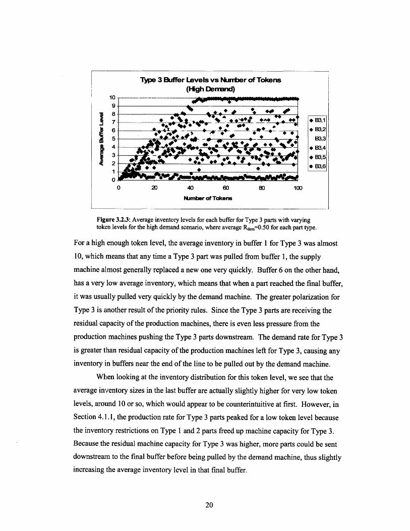
3.2.1, 3.2.2, and 3.2.3 show the average inventory levels for each individual buffer for
Type 1, Type 2, and Type 3 respectively in the high demand scenario.

Type I Buffer Levels vs Number of Tokens(High Dermnd)
In ____---- -
Figure 3.2.1: Average inventory levels for each buffer for Type 1 parts with varyingtoken levels for the high demand scenario, where average Rdem=0. 50 for each part type.
The graph in Figure 3.2.1 shows that the inventory distribution favors the
downstream buffers, especially for lower token levels. This means that the last
buffer in the line will generally have higher average inventory than buffers 1-5,
buffer 5 will have higher average levels than buffers 1-4, and so on. Since Type 1
parts receive the highest priority, the machine capacities are focused on Type 1
parts first. Thus, when a Type 1 part enters the system through a supply machine,
the production machines push it down to the last buffer, where it reaches a
bottleneck and sits until it is pulled by the Type 1 demand machine.
Since the number of tokens provides the upper limit on the inventory in
the system and the distribution favors downstream buffers, we see that as we
increase the number of tokens, the buffers furthest downstream fill up close to the
their capacities first. As we continue to increase token levels, the inventory
distribution works its way backward, filling upstream buffers one by one until all
the buffers are nearly full. The graph shows that for every increment of 10
tokens, there is a sharp increase in the average inventory level for a new buffer.
After increasing the token level by 10, the average inventory for that buffer then
reaches a plateau at a level similar to the downstream buffers. Thus, we can
expect that for parts that are achieving machine throughput rates that are higher
than the dermand rate for those parts, the inventory distribution will favor
9
6- - ____ B1,2
5-. 1 B1,31
4 B1,4
3 ."B1,52 " - -. B1,6
0-0 20 40 60 80 100
Number of Tokens

downstream buffers, especially when applying a more stringent control on the
inventory level by only allowing the system a low level of tokens.
When relating the inventory distribution and token levels back to the
production rates of type 1 parts, we can understand why the production rate
leveled off when the token level was only 30 parts. In the graph for average
inventory, we see that when the token level was about 30 parts, the average
inventories in the last and next to last buffers were each approximately 8 parts.
With inventory levels that high in the last buffers, there is almost always a part
available to be pulled by a demand machine in the up state. This means that only
the demand rate would be limiting production rate for a high priority part, since
the inventory level allowed is high enough.
The inventory distributions for the Type 2 and Type 3 parts show some clear
distinctions from the Type 1 distribution, largely due to the priority rules set in place for
the production machines. While the Type 1 inventory distribution favors downstream
buffers, the Type 2 and 3 distributions in Figures 3.2.2 and 3.2.3 favor upstream buffers.
This means that buffer 1 generally has more inventory than buffers 2-6, buffer 2 has more
inventory than buffers 3-6, and so on. With most of the production machine capacity
going to the Type 1 parts, there is not enough capacity left to keep pushing Type 2 and
Type 3 parts downstream. While the Type 1 inventory buffers appeared to fill up one at a
time for an increasing number of tokens, the inventory levels in each of the Type 2 and 3
buffers appeared to increase linearly with the number of tokens until they each stabilized
at their respective maximum inventory level.

Type 2 Buffer Levels vs Nunber of Tokens(High Denmnd)
-in
9
"7
6543210
0 20 40 60 80 100
NUmber of Tokens
Figure 3.2.2: Average inventory levels for each buffer for Type 2 parts with varyingtoken levels for the high demand scenario, where average Rdem=0. 50 for each part type.
As with the Type 1 inventory distribution and production rates, we see some
relationships between the distribution and output for Type 2. In the high demand
scenario, the Type 2 production rate reached a plateau when the number of tokens was
about 40. In Figure 3.2.2 above, we see that the average inventory levels for last two
buffers in the line stabilized at that same number of tokens. As for Type 1, when the
downstream buffers reached their peak average inventory level, there is a higher
probability of Type 2 inventory being available to be pulled when the demand machine
was up, resulting in higher Type 2 output. Increasing the token level beyond 40,
however, does not provide gains in production because the average inventory levels in the
last two buffers do not increase any more.
Overall, in the high demand scenario, the behaviors of the inventory distributions
for Type 2 and Type 3 were fairly similar, but the polarization of the inventory was
noticeably higher for Type 3 as seen below in Figure 3.2.3. For Type 2, the average
inventories of each of the buffers were closer to each other than for Type 3.
* B21
+ B2,2
* B2,4
SB2,5.. . .. .. . .. . .
I •
Type 3 Buffer Levels vs Nuimber of Tokens(High Demand)
1u
9876
543210
* B3,1* B3,2
83,3
* 83,4*B83,5
* 83,6
0 20 40 60 80 100
Number of Tokens
Figure 3.2.3: Average inventory levels for each buffer for Type 3 parts with varyingtoken levels for the high demand scenario, where average Rdem=0. 5 0 for each part type.
For a high enough token level, the average inventory in buffer 1 for Type 3 was almost
10, which means that any time a Type 3 part was pulled from buffer 1, the supply
machine almost generally replaced a new one very quickly. Buffer 6 on the other hand,
has a very low average inventory, which means that when a part reached the final buffer,
it was usually pulled very quickly by the demand machine. The greater polarization for
Type 3 is another result of the priority rules. Since the Type 3 parts are receiving the
residual capacity of the production machines, there is even less pressure from the
production machines pushing the Type 3 parts downstream. The demand rate for Type 3
is greater than residual capacity of the production machines left for Type 3, causing any
inventory in buffers near the end of the line to be pulled out by the demand machine.
When looking at the inventory distribution for this token level, we see that the
average inventory sizes in the last buffer are actually slightly higher for very low token
levels, around 10 or so, which would appear to be counterintuitive at first. However, in
Section 4.1.1, the production rate for Type 3 parts peaked for a low token level because
the inventory restrictions on Type 1 and 2 parts freed up machine capacity for Type 3.
Because the residual machine capacity for Type 3 was higher, more parts could be sent
downstream to the final buffer before being pulled by the demand machine, thus slightly
increasing the average inventory level in that final buffer.
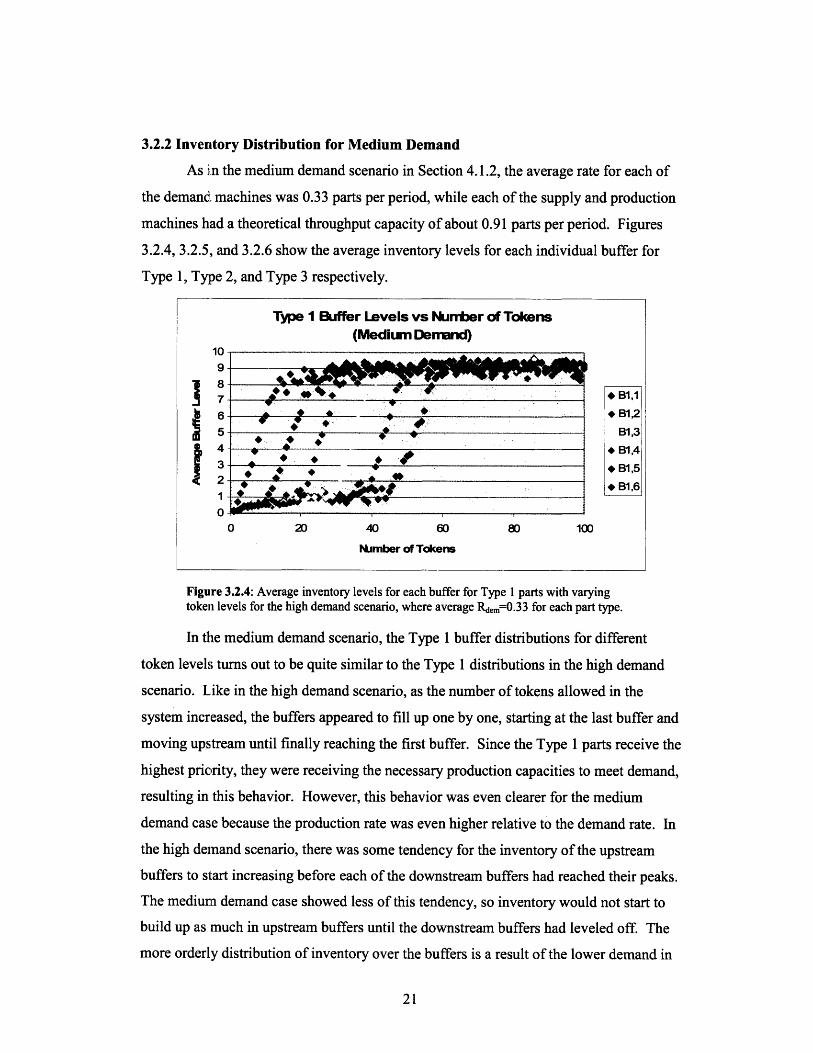
3.2.2 Inventory Distribution for Medium Demand
As in the medium demand scenario in Section 4.1.2, the average rate for each of
the demand machines was 0.33 parts per period, while each of the supply and production
machines had a theoretical throughput capacity of about 0.91 parts per period. Figures
3.2.4, 3.2.5, and 3.2.6 show the average inventory levels for each individual buffer for
Type 1, Type 2, and Type 3 respectively.
Type 1 Buffer Levels vs Number of TokensI(Meriu mm Deumand
lU
9
7
54321U
" B1,1
* B1,2
B1,3
* B1,4
* B1,5
* B1,6
0 20 40 60 80 100INUmber of Tokens
Figure 3.2.4: Average inventory levels for each buffer for Type 1 parts with varyingtoken levels for the high demand scenario, where average Rdem=0. 33 for each part type.
In the medium demand scenario, the Type 1 buffer distributions for different
token levels turns out to be quite similar to the Type 1 distributions in the high demand
scenario. Like in the high demand scenario, as the number of tokens allowed in the
system increased, the buffers appeared to fill up one by one, starting at the last buffer and
moving upstream until finally reaching the first buffer. Since the Type 1 parts receive the
highest priority, they were receiving the necessary production capacities to meet demand,
resulting in this behavior. However, this behavior was even clearer for the medium
demand case because the production rate was even higher relative to the demand rate. In
the high demand scenario, there was some tendency for the inventory of the upstream
buffers to start increasing before each of the downstream buffers had reached their peaks.
The medium demand case showed less of this tendency, so inventory would not start to
build up as much in upstream buffers until the downstream buffers had leveled off. The
more orderly distribution of inventory over the buffers is a result of the lower demand in
fff·i•| h m1r0 1•ll •I III\

this scenario. Since the demand rate is lower, the pressure from the production machines
pushing the parts downstream is higher relative to the pulling pressure from the demand
machines. Thus, for a given token level, parts are pushed into the downstream buffers
and spend more time sitting there before being pulled, rather than spending as much
relative time in the upstream buffers. This results in less creeping of the average
inventory levels upstream until all of the downstream buffers have been filled to their
peak levels.
The Type 2 inventory distributions for the medium demand scenario show some
important distinctions from the high demand scenario. In medium demand scenario, we
see what appears to be a transition in behavior from what we saw in the Type 1 and the
Type 2 distribution behaviors for high demand. Figure 3.2.5 below shows how the
inventory distribution varied with token level.
Type 2 Buffer Levels vs Nuntmer of Tokens(Medium Denrrnd)
iU
98
210
* 82,1
* B2,2
S82,4
* B2,6
0 20 40 60 80 100
NUmber of Tokens
Figure 3.2.5: Average inventory levels for each buffer for Type 2 parts with varyingtoken levels for the high demand scenario, where average Rdem=0. 33 for each part type.
In the high and medium demand scenarios, we saw that the Type 1 inventory
levels were more concentrated in downstream buffers. However, the high demand
scenario had Type 2 inventory levels favoring upstream buffers for all token levels. The
medium demand scenario shown in Figure 3.2.5 above, shows a transition between these
two different behaviors. For lower token levels, the distribution of Type 2 inventory
favors downstream buffers, yet it favors upstream buffers for higher token levels. Since

demand is lower in this scenario, when the token level is high, the pulling pressure from
the demand machines is lower relative to the pushing pressure on Type 2 parts from the
production machines, because the Type 2 parts are receiving less residual capacity from
the production machines than they do for lower token levels. For lower token levels,
however, the Type 2 parts receive more of the production capacity, causing them to
behave more like Type 1 parts in the way that inventory is pushed downstream.
The effect of the number of tokens on inventory distribution for Type 3 in the
medium demand case shows a similar behavior to that of Types 2 and 3 in the high
demand case, as shown in Figure 3.2.6 below.
Type 3 Buffer Levels vs Number of Tokens(Medium Derand)
1U
987
S6543210
* B3,1
" B3,2
B3,3
* B3,4
* B3,5
* B3,6
0 100
NurImber of Tokens
Figure 3.2.6: Average inventory levels for each buffer for Type 3 parts with varyingtoken levels for the high demand scenario, where average Rd~m=0.33 for each part type.
With the lower demand rate, the residual capacity of the production machines for
Type 3 is higher, since production rates on Type 1 and 2 are limited by their demand
rates. The greater residual capacity available for Type 3 causes the polarity of the
inventory distribution to be less than it was in the high demand scenario. Figure 3.2.6
shows that the average inventory for buffer 6 is noticeably higher than in the high
demand scenario that we saw in Figure 3.2.3. This is a result of the increased
downstream pressure from the production machines as well as a lower pulling pressure
from the demand machine, since the average demand rate is lower.
40 60100
0 100

3.2.3 Inventory Distribution for Low Demand
As in the low demand scenario in Section 4.1.3, the average rate for each of the
demand machines was 0.167 parts per period, while each of the supply and production
machines again had a theoretical throughput capacity of about 0.91 parts per period.
Figures 3.2.7, 3.2.8, and 3.2.9 show the average inventory levels for each individual
buffer for Type 1, Type 2, and Type 3 respectively.
Figure 3.2.7: Average inventory levels for each buffer for Type 1 parts with varyingtoken levels for the high demand scenario, where average Rdem=0.1 6 7 for each part type.
The inventory distribution for the Type 1 parts in the low demand scenario differs
only slightly from the medium and high demand scenario, in the same way that the
medium demand scenario differed from the high demand scenario. As for the other
scenarios, we see here that the distribution of inventory favors downstream buffers.
However, this tendency is even clearer for the low demand scenario. We see even less
creeping of inventory into the upstream buffers. On average, there is very little inventory
in a buffer until the token level is high enough to fill all of the buffers that are
downstream from that point. The Type 2 buffer shows a very similar behavior in Figure
3.2.8 below.
Type 1 Buffer Levels vs Nuinter of Tokens(Low Derrand)
10 -9-o
6-5 .4
3(2-
* B1,1
* B1,2
B1,3
" B1,4
" 81,5
* B1,6
0 20 40 60 80 100
NUmber of Tokens

Type 2 Buffer Levels vs Number of Tokens(Low Demand)
10
0 20 40 60 80 100
Number of Tokens
Figure 3.2.8: Average inventory levels for each buffer for Type 2 parts with varyingtoken levels for the high demand scenario, where average Rdem=0.167 for each part type.
With demand rates so low in this scenario, the Type 1 parts only consume a small
portion of the capacity of the five production machines. This leaves enough capacity for
the Type 2 parts to meet the demand rates, causing an inventory distribution behavior
similar to each of the Type 1 scenarios. The average inventory in a given buffer does not
increase by much until the token level is high enough to fill all of the downstream
buffers. The Type 2, and also the Type 3, distributions do differ slightly from Type 1
behavior in that the inventory levels of upstream buffers do increase slightly before all of
the downstream buffers have been filled. Also, for high token levels, the inventories in
the upstream buffers are slightly higher than the downstream buffers for the lower
priority types. The Type 1 parts are still receiving slightly more of the production
machine capacity than the Type 2 and 3 parts, causing more pressure pushing parts
downstream for the higher priority parts. Since the downstream pressure is less for the
lower priority part types, the upstream levels remain slightly higher for high token levels.
7-
S6-5 -
3-( 2-
4 _ _
* B2,4
SB2,6" B2,5" 82,6.. . .. . ... ..

Type 3 Buffer Levels vs iNumber of Tokens
IL
9
76543
2
1
0
kL.LW L.I II IUJ
* B3,1
* B3,2
B3,3
" B3,4
" B3,50 MRf
0 20 40 60 80 100
NUmber of Tokens
Figure 3.2.9: Average inventory levels for each buffer for Type 3 parts with varyingtoken levels for the high demand scenario, where average Rem=0. 167 for each part type.
When relating the inventory distribution to the output for the different types, we
find that the peak output rates correspond to the peak average inventory levels in the last
buffers in the same way that they did for the high and medium demand scenarios. The
peak production rates stabilized at token levels of about 15 for all three part types, which
corresponds to the token level where the average inventory of the last buffer for each of
the types leveled off at its maximum level.
In the low demand scenario, we see an interesting behavior of in the random
variation of the average inventory levels for the buffers after they have reached their
stable levels. When comparing the variation in the levels for each of the buffers over the
different part types, we find that the lower priority types show larger random variation
than the higher priority types. Even for the highest priority Type 1 parts, the system has
some built in random variation in inventory levels due to the randomness in the up and
down states of all of the machines. The Type 2 parts see increased random variation
from the system because they receive the residual capacity from the Type 1 parts, so the
randomness of the system is compounded with the randomness from the Type 1 parts.
The Type 3 parts face even greater random variation because they face the randomness
from the system plus the compounded randomness of the Type 1 and Type 2 parts. This
behavior is important to recognize because the randomness affects how accurately and
, L~
confidently we can predict inventory distribution for each part type. With higher random
variation for the lower priority parts, accurately predicting the inventory distribution
becomes more difficult. Thus designing the production system and inventory controls for
lower priority parts also becomes more difficult.
4. Conclusion
This research studies the effect of maximum allowed inventory level through
CONWIP control on the performance of a flexible manufacturing system producing
different part types according to a strict priority rule. The CONWIP control method
applied individual limits on the system inventory level for each of the part types. The
individual token limits were set at the same level as they were varied simultaneously
while running simulations to determine the average per period output and average
inventory level of each buffer for each part type.
4.1 Production Rates Intuition
In a flexible production system, the spread between the production rates of the
different part types is larger for higher levels of demand. Given the same demand level,
the spread between production levels also increases with token level, as the throughput
rate of the higher priority parts are less constrained by limits on inventory. Interestingly,
for high demand rates, the highest production rate of the lowest priority type actually
peaks at a very low token level because it receives the largest residual capacity when
throughput of higher priority parts are constrained by inventory limits. When the demand
rates decrease from high levels, the production rates of the higher priority parts decrease
while the lower priority part types actually tend to increase due to larger residual
production machine capacities for those types. As demand rate continues to decrease, the
production rates of all the part types eventually meet at the same level and then decrease
together with further drops in demand rates. For low levels of demand, the average
output of each of the part types move together with changing token levels. The output of
each part type increases with token level until reaching a plateau at a fairly low token
level. Also, the token level necessary to reach the maximum production rate was lower

for lower demand rates. Intuitively, the inventory in the system does not need to be as
high if demand rates are lower in relation to the throughput capacity of the system.
4.2 Inventory Distribution Intuition
The application of the CONWIP controls showed some interesting implications
for the inventory distributions in different demand scenarios. The inventory distributions
also appeared to have implications on the output rates. For each part type in each
scenario, the production levels consistently reached their maximum level when the
furthest downstream buffer also reached its maximum level. For each demand level, the
part types that received enough machine capacity to meet each of their demand rates
showed a similar behavior in their inventory distributions. These types tend to fill their
buffers one at a time, starting with the buffers furthest downstream and working
backwards up the line from there. On the other hand, the types not receiving enough
capacity from the production machines to meet their demand rates would tend to have
higher inventory in the upstream buffers.
4.3 Future Research
With the intuitions developed in this research, production managers can more
intelligently design flexible production lines with inventory controls to achieve the
desired results. The intuition also serves as a good starting point for further research in
design optimization for systems using similar control methods. Eventually, for a given
production system, a manager should be able to balance inventory costs, machine
capacities, supply rates, and demand rates to achieve an optimum production system
design.

Appendix
A.1 Numlber of Time Periods in Simulation
When running the simulation, it is important to run it for a long enough time that
it reaches a steady state production rate and inventory distribution. This way we are
measuring the steady state behaviors instead of any behavior that is affected by ramping
up time in the transient periods. For this research, we ran the simulation for a length of
10800 time periods, and recorded the inventory levels and production output for the last
3600 periods. After running some initial trials, we compared the results of simulations as
long as 21600 periods to ones as short as 3600 periods and found that over a
measurement window of 3600 periods for each simulation length, we obtained the same
behavior. The simulations, however, showed different results for trials up to 3600
periods than for longer ones. When looking at behavior beyond the initial 3600 periods,
the results became consistent, so the ramp up time is approximately 3600.

Bibliography
[1] K.E. Stecke. Design, planning, scheduling, and control problems of flexible
manufacturing systems. Annals of Operations Research, 3(1): 1-12, January 1985.
[2] H. Tempelmeier and H. Kuhn. Flexible Manufacturing Systems: Decision Support
for Design and Operation. Wiley-Interscience, New York, NY 1993.
[3] Y.J. Jang. Mathematical Modeling and Analysis of Flexible Production Lines. PhD
thesis, Massachusetts Institute of Technology, Laboratory for Manufacturing and
Productivity, June 2007.