journal of hydrology - srs.fs.usda.gov · in general, our results showed ... of climate and...
TRANSCRIPT

Journal of Hydrology 424–425 (2012) 217–237
Contents lists available at SciVerse ScienceDirect
Journal of Hydrology
journal homepage: www.elsevier .com/ locate / jhydrol
Revisiting the homogenization of dammed rivers in the southeastern US
Ryan A. McManamay a,⇑, Donald J. Orth a, Charles A. Dolloff b
a Department of Fish and Wildlife Conservation, Virginia Tech, Blacksburg, VA 24061, USAb USDA Forest Service, Department of Fish and Wildlife Conservation, Virginia Tech, Blacksburg, VA 24061, USA
a r t i c l e i n f o
Article history:Received 23 May 2011Received in revised form 1 December 2011Accepted 4 January 2012Available online 11 January 2012This manuscript was handled by GeoffSyme, Editor-in-Chief, with the assistance ofJohn W. Nicklow, Associate Editor
Keywords:Hydrologic alterationFlow classificationDam regulationNatural flow regimeWatershed disturbance
0022-1694/$ - see front matter Published by Elsevierdoi:10.1016/j.jhydrol.2012.01.003
⇑ Corresponding author. Present address: Oak Ridgronmental Sciences Division, Bldg. 1504, Oak Ridge, TTel.: +1 540 574 9154.
E-mail addresses: [email protected] (R.A.(D.J. Orth), [email protected] (C.A. Dolloff).
s u m m a r y
For some time, ecologists have attempted to make generalizations concerning how disturbances influ-ence natural ecosystems, especially river systems. The existing literature suggests that dams homogenizethe hydrologic variability of rivers. However, this might insinuate that dams affect river systems similarlydespite a large gradient in natural hydrologic character. In order to evaluate patterns in dam-regulatedhydrology and associated ecological relationships, a broad framework is needed. Flow classes, or groupsof streams that share similar hydrology, may provide a framework to evaluate the relative effects of damregulation on natural flow dynamics. The purpose of this study was to use a regional flow classification asthe foundation for evaluating patterns of hydrologic alteration due to dams and to determine if theresponse of rivers to regulation was specific to different flow classes. We used the US Geological Survey(USGS) database to access discharge information for 284 unregulated and 117 regulated gage records. Foreach record, we calculated 44 hydrologic statistics, including the Indicators of Hydrologic Alteration. Weused a sub-regional flow classification for eight states as a way to stratify unregulated and regulatedstreams into comparable units. In general, our results showed that dam regulation generally had strongereffects on hydrologic indices than other disturbances when models were stratified by flow class; how-ever, the effects of urbanization, withdrawals, and fragmentation, at times, were comparable or exceededthe effects of dam regulation. In agreement with the existing literature, maximum flows, flow variability,and rise rates were lower whereas minimum flows and reversals were higher in dam regulated streams.However, the response of monthly and seasonal flows, flow predictability, and baseflows were variabledepending on flow class membership. Principal components analysis showed that regulated streamsoccupied a larger multivariate space than unregulated streams, which suggests that dams may nothomogenize all river systems, but may move them outside the bounds of normal river function. Ulti-mately, our results suggest that flow classes provide a suitable framework to generalize patterns inhydrologic alterations due to dam regulation.
Published by Elsevier B.V.
1. Introduction
Of the many disturbances that negatively impact the integrityof aquatic ecosystems, dam regulation results in the most exten-sive damages (Vitousek et al., 1997). Dams reduce the hydrologicvariability of river systems that is responsible for forming andmaintaining the habitats to which river biota are adapted (Poffet al., 1997; Trush et al., 2000; Bunn and Arthington, 2002). A gen-eral rule of thumb is that dams tend to ‘‘homogenize’’ river flowsacross geographical scales, leading to a loss of habitat variability(Poff et al., 2007) and a homogenization of river fauna (Moyleand Mount, 2007). For example, the majority of studies show that
B.V.
e National Laboratory, Envi-N 37831-6351, United States.
McManamay), [email protected]
following dam regulation, minimum flow magnitudes increasewhereas maximum flow magnitudes decrease (Magilligan andNislow, 2001, 2005; Pyron and Neumann, 2008; Poff et al., 2007).Other general patterns include decreased rise and fall rates ofhydrographs and increases in reversals (positive or negativechanges from 1 day to the next) (Magilligan and Nislow, 2001,2005; Pyron and Neumann, 2008). However, there are exceptionsto the rule that dams influence all rivers the same. This may beespecially true for rivers in the southeastern US that differ in termsof climate and geomorphology. For example, the effect of dams onmonthly flows, the frequency of flows, and the timing of flows canvary due to dam type, dam operations, dam storage capacity, andare specific to different regions (Richhter et al., 1996; Magilliganand Nislow, 2005; Pyron and Neumann, 2008).
One of the obvious and more robust approaches for determiningthe effect of dam regulation on stream flows is by comparison ofpre- and post-regulation datasets, which has been conductedextensively (Richhter et al., 1996; Magilligan and Nislow, 2001,

218 R.A. McManamay et al. / Journal of Hydrology 424–425 (2012) 217–237
2005; Poff et al., 2007; Pyron and Neumann, 2008; Gao et al.,2009). Using paired pre- and post-regulation data comparisonsfor individual drainages is a preferred method because it controlsfor differences in basin size and other confounding factors withthe exception of temporal shifts in climate regimes. In addition,the criteria for selecting appropriate gages for such analyses canbe quite strict (e.g. adequate pre- and post-regulation information,usually regulated by no more than one dam, and basins are not dis-turbed by factors other than dam regulation). Confining analyses tothese criteria results in reduced sample size, reduced spatial reso-lution, and ultimately, a loss of information. In basins characterizedby cumulative anthropogenic stressors, it may be difficult toclearly define the impacts of each stressor; thus, time-series anal-ysis can identify break points or apparent changes in stream flowpatterns attributable to different anthropogenic stressors (Vogland Lopes, 2009). However, these specific analyses are usually lim-ited to individual basins. Ultimately, it appears there is a need for abroader framework that provides an improved, alternative meansof assessing the influence of dam regulation on stream hydrology.Such a framework could stratify basins into comparable unitsthereby eliminating the need, but allowing the inclusion, of pre-and post regulation information. However, the framework wouldalso have to control for differences among basins, such as basinsize, and account for cumulative hydrologic disturbances. Addi-tionally, a similar framework would also be useful as structurefor evaluating the effect of hydrologic alterations on aquatic biota,especially since there is limited information to develop quantita-tive relationships between flow alterations and ecological re-sponses (Carlisle et al., 2010b; Poff and Zimmerman, 2010).
Geographic or geomorphic settings provide some context forevaluating hydrologic variability (Poff et al., 2006b) or patterns inhydrologic alterations (Poff et al., 2007). For example, Poff et al.(2007) used 16 regions of the US to evaluate patterns in hydrologicalterations. Although the study did show a tendency of dams tohomogenize natural flow variability, the magnitude and directionin which dams influence flow dynamics were region-specific. An-other approach to stratify hydrologic alteration studies is by classi-fying streams into groups of similar flow characteristics (Arthingtonet al., 2006; Poff et al., 2010) (Fig. 1). Classifications of rivers based onstream discharge data alone have been conducted at the continentalscale (Poff and Ward, 1989; Poff, 1996; Kennard et al., 2010b), the re-gional scale (McManamay et al., 2011a), and for individual states(Kennen et al., 2007; Turton et al., 2008; Kennen et al., 2009). Theseflow classes can be used as ecologically-meaningful managementunits by which environmental flow standards are formed or as aframework for evaluating hydrologic alterations (Arthington et al.,2006; Poff et al., 2010). We hypothesize that hydrologic alterationsdue to dam regulation may be specific to a river’s natural hydrologicpredisposition (i.e. flow class membership). Flow classes representgroups of streams that share similar soils, climate, and geomorphol-ogy (McManamay et al., 2011b); thus, they should control for someof the differences among basins, thereby eliminating the necessity touse only gages with adequate pre- and post-regulation data. Forexample, a regulated river can be classified to a group of streams thatshare similar unregulated or undisturbed flow characteristics eitherby using pre-disturbance hydrologic information or by using land-scape characteristics (Fig. 1). Flow classes then become the organi-zational structure by which hydrologic alterations are measured(Fig. 1).
The purpose of this study was to use a regional flow classifica-tion in the southeastern US as the foundation for evaluating pat-terns of hydrologic alteration due to dams. We focus our studyon a region of the southeastern US because of the current and pro-posed increases in population and the multiple stresses on surfacewater demands (Sun et al., 2008). In addition, the Southeast has thehighest density of dams in the US (Graf, 1999). Understanding how
multiple factors affect stream flow availability, timing, duration,and frequency is critical to adapting policies to mitigate the effectsof current and future impacts. Although we focus primarily on theeffect of dam regulation, other disturbances, such as withdrawalsand urbanization, should be considered. Lastly, it may be informa-tive to understand how dam regulation influences the overall var-iability in river systems in order to adequately judge whether theremay be a homogenizing effect. Our specific objectives were to (1)compare pre/post-regulation stream flow records as standard pro-tocol to provide initial evidence for class-specific hydrologic alter-ations caused by dams and to warrant further investigation, (2)isolate the effects of dam regulation from other causes of hydro-logic disturbance within flow classes using all stream gages,regardless of pre/post regulation hydrologic data, (3) evaluatehow dam regulation influences the overall variability in river sys-tems, and (4) generalize patterns in hydrology caused by damsacross and within different flow classes.
2. Study region
The study region includes all or part of 8 states of the southeast-ern US (Georgia, Kentucky, Maryland, North Carolina, SouthCarolina, Tennessee, Virginia, and West Virginia). The regionextends west to east from the central Appalachian Mountains tothe coastal plain (Atlantic Ocean) and from north to south fromthe Potomac River basin in Maryland to the Savannah River basinin Georgia (Fig. 2). Basins in our study averaged 2727 km2 and ran-ged from 12.8 to 29,952 km2. Maximum elevations for each basinrange from 15 m in the coastal plain to 2028 m in the mountainousregion and average annual precipitation ranges from 93 to 207 cm.Average slopes range from 0% to 35%, with the highest in themountainous regions. Forest coverage is the dominate land-usecategory in most basins averaging 67% (10–100%). Agricultureaverages 18% (0–65%) whereas urbanization averages 7% (0–36%).Inceptisols soils dominate the moist climates of the mountainousareas whereas ultisols dominate the majority of the coastal plainand piedmont, with the exception of a distinct band of alfisols (clayrich) in the center of the piedmont.
3. Methods
3.1. Overview
We present a 7-step framework as a means to assess and gener-alize the influence of dam regulation on stream hydrology (Fig. 1).The basic principles and theoretical basis for the conceptual modelwere taken and modified from ideas presented by Arthington et al.(2006) and Poff et al. (2010). In general, the process includes com-piling streams influenced and uninfluenced by dam regulation,stratifying basins in comparable units, accounting for cumulativehydrologic disturbances, and then isolating the effects of dam reg-ulation. The first step includes assembling unregulated streamgages (not regulated by dams) and dam-regulated stream gages.This also includes compiling hydrologic information for regulatedstream gages with periods of record proceeding dam regulation.From the group of unregulated stream gages, reference gages areselected that represent relatively undisturbed streams and thenused in a flow classification (step 2). Flow classes are groups ofstreams that share similar natural hydrology; thus, they providea stratified approach to evaluate hydrologic alterations or depar-tures from natural baseline conditions. Hydrologic information orlandscape characteristics are then used to develop predictive toolsto assign streams to an appropriate flow class (step 3). Dependingon the availability of pre-disturbance hydrologic data, unregulatedstreams (those not included in the classification) and regulated
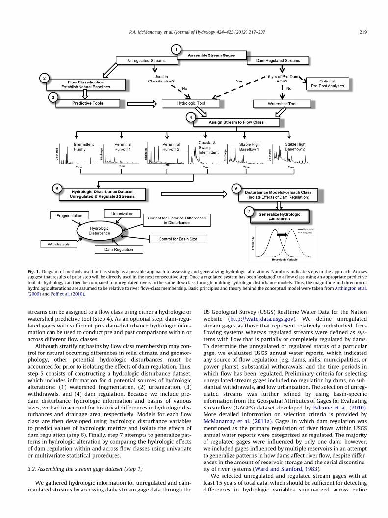
Fig. 1. Diagram of methods used in this study as a possible approach to assessing and generalizing hydrologic alterations. Numbers indicate steps in the approach. Arrowssuggest that results of prior step will be directly used in the next consecutive step. Once a regulated system has been ‘assigned’ to a flow class using an appropriate predictivetool, its hydrology can then be compared to unregulated rivers in the same flow class through building hydrologic disturbance models. Thus, the magnitude and direction ofhydrologic alterations are assumed to be relative to river flow-class membership. Basic principles and theory behind the conceptual model were taken from Arthington et al.(2006) and Poff et al. (2010).
R.A. McManamay et al. / Journal of Hydrology 424–425 (2012) 217–237 219
streams can be assigned to a flow class using either a hydrologic orwatershed predictive tool (step 4). As an optional step, dam-regu-lated gages with sufficient pre- dam-disturbance hydrologic infor-mation can be used to conduct pre and post comparisons within oracross different flow classes.
Although stratifying basins by flow class membership may con-trol for natural occurring differences in soils, climate, and geomor-phology, other potential hydrologic disturbances must beaccounted for prior to isolating the effects of dam regulation. Thus,step 5 consists of constructing a hydrologic disturbance dataset,which includes information for 4 potential sources of hydrologicalterations: (1) watershed fragmentation, (2) urbanization, (3)withdrawals, and (4) dam regulation. Because we include pre-dam disturbance hydrologic information and basins of varioussizes, we had to account for historical differences in hydrologic dis-turbances and drainage area, respectively. Models for each flowclass are then developed using hydrologic disturbance variablesto predict values of hydrologic metrics and isolate the effects ofdam regulation (step 6). Finally, step 7 attempts to generalize pat-terns in hydrologic alteration by comparing the hydrologic effectsof dam regulation within and across flow classes using univariateor multivariate statistical procedures.
3.2. Assembling the stream gage dataset (step 1)
We gathered hydrologic information for unregulated and dam-regulated streams by accessing daily stream gage data through the
US Geological Survey (USGS) Realtime Water Data for the Nationwebsite (http://waterdata.usgs.gov). We define unregulatedstream gages as those that represent relatively undisturbed, free-flowing systems whereas regulated streams were defined as sys-tems with flow that is partially or completely regulated by dams.To determine the unregulated or regulated status of a particulargage, we evaluated USGS annual water reports, which indicatedany source of flow regulation (e.g. dams, mills, municipalities, orpower plants), substantial withdrawals, and the time periods inwhich flow has been regulated. Preliminary criteria for selectingunregulated stream gages included no regulation by dams, no sub-stantial withdrawals, and low urbanization. The selection of unreg-ulated streams was further refined by using basin-specificinformation from the Geospatial Attributes of Gages for EvaluatingStreamflow (GAGES) dataset developed by Falcone et al. (2010).More detailed information on selection criteria is provided byMcManamay et al. (2011a). Gages in which dam regulation wasmentioned as the primary regulation of river flows within USGSannual water reports were categorized as regulated. The majorityof regulated gages were influenced by only one dam; however,we included gages influenced by multiple reservoirs in an attemptto generalize patterns in how dams affect river flow, despite differ-ences in the amount of reservoir storage and the serial discontinu-ity of river systems (Ward and Stanford, 1983).
We selected unregulated and regulated stream gages with atleast 15 years of total data, which should be sufficient for detectingdifferences in hydrologic variables summarized across entire

Fig. 2. Map of the study region in the southeastern United States. Upper and lower limits of study region are represented by the Potomac and Savannah River basins,respectively. Unregulated and regulated rivers are plotted according to their respective natural flow classes created by McManamay et al. (2011a). Gages marked with ‘B’ or‘A’ represent gages that have pre- and post-regulation gage information. ‘B’ indicates that the point represents gage data taken from pre-regulation time periods whereas ‘A’represents post-regulation gage data.
220 R.A. McManamay et al. / Journal of Hydrology 424–425 (2012) 217–237
periods of record and not evaluating changes in hydrologic vari-ables across temporal scales (Kennard et al., 2010a). We used somegage records with non-continuous or missing data as long as atleast 15 total years were represented. For regulated stream gagesthat had at least 15 years of pre-impoundment data, we selecteddata from periods of time with no regulated flow to include inour analysis as unregulated status. Overall, 284 unregulated
stream gage records and 117 regulated stream gage records with15 years of record were isolated. Of the unregulated stream re-cords, 49 consisted of streams that are currently regulated by damsbut had at least 15 years of pre-dam disturbance information. Sim-ilarly, of the regulated gage records, 49 of the records consisted ofpost-regulation information. Gages with at least 15 years of pre-and post-regulation data were used in Section 3.4.

R.A. McManamay et al. / Journal of Hydrology 424–425 (2012) 217–237 221
Mean daily and annual peak flow data were downloaded fromthe USGS Realtime Water Data for the Nation website for 401stream gage records (284 unregulated and 117 regulated records).Hydrologic statistics were calculated for each stream record usingthe Hydrologic Index Tool (HIT) software available through USGS(Henriksen et al., 2006). Daily and peak flow gage data for the en-tire period of record were imported into HIT, which calculates the171 hydrologic indices reported in Olden and Poff (2003). The indi-ces are grouped into five categories of flow: magnitude (n = 94),frequency (n = 14), duration (n = 44), timing (n = 10), and rate ofchange (n = 9) with each category having low, average, and highflow subcategories (Richhter et al., 1996; Olden and Poff, 2003). Be-cause the 171 hydrologic variables are correlated and highlyredundant (Olden and Poff, 2003), we originally reduced the data-set to 40 variables (Table 1), which included the 33 Indicators ofHydrologic Alteration (IHA) (Richhter et al., 1996), three Environ-mental Flow Component (EFC) indices (Mathews and Richter,2007), and 4 of the variables found in Poff (1996). Olden and Poff(2003) showed that the IHA variables and EFC variables explainedthe majority of variation in all 171 published hydrologic indices.Because several of the IHA variables were not calculated for somestreams and would limit our multivariate analyses, we includedfour additional variables from Poff (1996) bringing the total num-ber of hydrologic variables to 44 (Table 1). All magnitude variablesand any variables related to magnitude were divided by the med-ian daily flow for each stream to standardize for differences in riversize, which is a commonly used approach when evaluating hydro-logic variability over spatial scales (Poff and Ward, 1989; Poff et al.,2006; Kennard et al., 2010b). We presume that standardization bymedian flow is a preferred method over standardization by drain-age area since hydrologic variables share non-linear relationshipswith drainage area (Leopold, 1994).
3.3. Flow classification, predictive tools, and assigning gages to flowclasses (steps 2–4)
Flow classifications have been proposed as a robust frameworkfor generalizing hydrologic alterations across regions by stratifyingbasins into comparable units (step 2, Fig. 1) (Arthington et al.,2006; Poff et al., 2010). For our region of interest, McManamayet al. (2011a) classified 292 streams into six distinct flow classesrepresenting differences in the magnitude, frequency, durationand rate of change in flow regimes. These classes provide thehydrologic baseline from which departures in flow due to distur-bance can be measured.
Predictive tools, or classification models, are commonly devel-oped to accompany hydrologic classifications as mechanisms used
Table 1Hydrologic indices include the 33 Indicators of Hydrologic Alteration (IHA) (Richhter et a2007), and eight indices used in Poff (1996). Hydrologic alteration models were built for 40some streams, additional variables were included in the principal components analysis (P
Flow variabilitya November flow 7-DJanuary flow December flow 30-February flow Minimum July flowb,c 90-March flow Base flow index LowApril flow Low pulse count No.May flow Low pulse variabilityb,c 1-DJune flow High pulse count 3-DJuly flow High pulse variabilityb,c 7-DAugust flow Flood frequencya,c 30-September flow 1-Day minimum 90-October flow 3-Day minimumc Flo
a Poff (1996).b EFC (Mathews and Richter, 2007).c Used in hydrologic alteration model but not PCA.d Used in PCA but not hydrologic alteration model.
to assign streams to appropriate classes (step 3, Fig. 1) (Kennenet al., 2007; Kennard et al., 2010b; Olden et al., 2011). Thesepredictive tools can be used to classify gaged streams not used inthe original classification or ungaged streams with sufficientclimate, soils, and toprographical information. In association withthe flow classification, McManamay et al. (2011a) developed ahydrologic classification tool, which consisted of five hydrologicvariables that could classify a stream gage to 1 of 6 flow classeswith 85% accuracy. In addition, McManamay et al. (2011b) builta watershed classification tool that accurately classified 74% ofstreams to their appropriate flow class using primarily soil andclimate variables. The watershed tool was built using the GAGESdataset (Falcone et al., 2010), which includes soils, topographic,and climate information summarized across the contributingwatershed upstream of each gage. The GAGES dataset includesinformation for 6785 USGS gages with at least 20 years of data,which included the regulated stream gages used in our study.
The next critical step in forming generalizations of dams affectflow dynamics is by assigning streams to a particular class (step 4,Fig. 1) (Arthington et al., 2006; Poff et al., 2010). The majority ofunregulated gage records in our dataset (n = 273 of 284) and someof the regulated gages with pre-regulated data (n = 38 of 117) wereused in the flow classification and thus, were already assigned to 1of 6 flow classes. For the remainder of unregulated (n = 11) andregulated (n = 78) gage records, we used one of the two predictivetools to assign gages to appropriate flow classes depending on theavailability of hydrologic data. For regulated streams with at least15 years of pre-regulation hydrologic information, we used thehydrologic classification tool to assign those gages to a flow class.Because the majority of regulated gages had inadequate pre-regu-lation hydrologic data, we used the watershed classification toolcreated by McManamay et al. (2011b) to assign gages to 1 of 6 flowclasses. One limitation of this approach is that some gages may bemisclassified. Because flow classes represent clouds or aggrega-tions in multivariate space, some streams within a particular classmay be located near border of an adjoining cloud and thus, moreprone to misclassification, which is a typical drawback from hard,centroid-based clustering (Jain, 2010). However, misclassificationrates are typically low and result in gages being assigned to flowclasses that share similar hydrology (McManamay et al., 2011b).For example, McManamay et al. (2011b) found that stable highbaseflow 1 (SBF1) streams share similar geographical extent andsimilar baseflow characteristics with stable high baseflow 2streams (SBF2). If SBF1 streams are classified inaccurately usingwatershed classification trees, they are typically misclassified asSBF2 streams. Thus, we hypothesize that classes that share similarhydrology might respond similarly to dam regulation.
l., 1996), three Environmental Flow Component (EFC) indices (Mathews and Richter,hydrologic variables. Because 6 of the 40 hydrologic variables were not calculated for
CA).
ay minimum Flood durationd
Day minimum Flow predictabilitya
Day minimum Seasonal flood predictabilitya
flow duration Seasonal predictability (low flow)a,d
of zero flow daysc Seasonal predictability (non-low flow)a,d
ay maximum Seasonal predictability (non-flooding)a,d
ay maximum Date of annual minimumay maximum Date of annual maximumDay maximum Rise rateDay maximum Fall rateod intervala Reversals

222 R.A. McManamay et al. / Journal of Hydrology 424–425 (2012) 217–237
3.4. Pre- and post-regulation analysis (optional step)
Because pre/post analyses have dominated the literature, wewanted to use this analysis to provide some justification that flowclasses can be used as a basis for evaluating hydrologic alterations.After all stream gages were classified to an appropriate class, wecalculated percent changes in 10 ecologically-relevant hydrologicvariables following dam regulation for the 49 gages with 15 yearseach of pre- and post-regulation data. We chose the 10 hydrologicvariables because they dominate studies which evaluated thehydrologic effects of dams using pre-post regulation information(Richhter et al., 1996; Magilligan and Nislow, 2001, 2005; Poffet al., 2007; Pyron and Neumann, 2008). We used unstandardizedvalues for hydrologic variables rather than those standardized bythe median daily flow for the before/after analysis because com-parisons were from the same basin. We sorted each pre-post anal-ysis by flow class and evaluated percent changes among differentflow classes using box plots.
3.5. Hydrologic disturbance dataset (step 5)
Determining the influence of dams on flow dynamics by usingonly gages with adequate pre- and post-regulation data may limitsample sizes and exclude important information in analyses. Forexample, only 49 of the 117 regulated gages in our study regionhad adequate pre-regulation data. Therefore, to increase samplesize, we evaluated gross differences in hydrologic variables be-tween regulated and unregulated streams, regardless of the avail-ability of pre-regulation information. One limitation of thisapproach is that gross comparisons may not account for differ-ences in watershed characteristics and other disturbance factorsbesides dam regulation.
In order to account for other hydrologic disturbances that mayconfound our analyses, we assembled a hydrologic disturbancedataset using the GAGES database, which includes 27 dam regula-tion variables, 11 hydrologic modification variables (e.g. withdraw-als), and a large suite of land-use metrics for 6785 stream gages inthe US (Falcone et al., 2010). Each variable represents a summaryfor each gage’s entire basin and not just values at each gage loca-tion. One challenge that arose with our dataset was that the valuesfor the hydrologic disturbance variables for each gage were basedon current conditions. Thus, disturbance values for gages with bothpre- and post-regulation records were similar. For example, damdisturbance variables, such as total dam storage, were based on2006 National Dam Inventory Data (USACE, 2011) whereas land-use variables, such as% urbanization and % fragmentation in thewatershed, were based using the 2001 National Land-Cover Data-set (NLCD). Freshwater withdrawal estimates came from 1995 to2000 county-level estimates from USGS datasets. Thus, to usehydrologic data from the pre-regulation time periods in our data-set, we had to correct for recent changes in water use, dam regula-tion, and land use. The GAGES dataset included changes in totaldam storage and dam density for each gage in every decade since1940, which allowed for easily correcting for differences in totalstorage in each basin. If the dam regulation time period was priorto 1930, then we assumed a value of 0 for both dam storage anddam density.
Historical values for withdrawals and land use were not asreadily available as dam regulation information. We used the2005 USGS national water report (Kenny et al., 2009) to evaluatechanges in withdrawals over time. Trends in water withdrawalswere available for each major water consumption category acrossthe US since 1950 (public supply, domestic, irrigation, livestock,industrial, and thermoelectric) (Supplementary material 1). Mostcategories showed general increases in water use since 1950 ex-cept for industrial uses (Supplementary material 1). We developed
linear regressions or second-order polynomial regressions on per-cent changes in withdrawals according to year for each category.The proportion of water use in each category was also availablefor each state (Supplementary material 2). Because water use indifferent consumption categories varies substantially from stateto state (Kenny et al., 2009), the percent changes in withdrawalswere weighted by water use in each category for each statedepending on the location of each gage. We then applied regres-sions for each gage based on the year since dam regulation to cor-rect withdrawal estimates. Thermoelectric withdrawals dominatedwater usage trends for most states and across the US; however,based on USGS annual water reports, thermoelectric usage is pat-chy and does not occur in every basin. Since accounting for ther-moelectric usage in each basin could heavily influence ourhistorical withdrawal estimates, we only included trends in ther-moelectric usage for gages in which the USGS water reports men-tioned some flow regulation due to power plants within the basin.
Historical trends in land use since 1950 were available for thesoutheastern US according to seven different level-3 ecoregions(Brown et al., 2005) (Supplementary material 3). We ran regres-sions for percent changes in each land-use category (% urban and% agriculture) for each ecoregion. We corrected for changes in % ur-ban and % agriculture land cover types using the year since damregulation depending on the ecoregion in which each gage was lo-cated. Watershed fragmentation is an index based upon the per-centage of undeveloped land (non-urban and non-agriculturalland – higher index values indicate more fragmentation (Falconeet al., 2010)). Because % agriculture showed relatively little change(0–21% decrease) compared to urbanization (33–103% increase),we used changes in % urban land cover to account for any changesin fragmentation.
One of the limitations in our analysis for correcting withdrawaland land-use estimates is that we assume patterns across the USand across entire ecoregions are representative of patterns withineach basin. Also, our corrected withdrawal and land cover esti-mates were highly dependent upon current estimates (correctedusing % change); thus, if withdrawal and urbanization is currentlyhigh within a particular basin, pre-regulation estimates should re-flect current high conditions. However, we do not expect that slightinaccuracies in assessing historical estimates would overwhelmour analyses since there are only 49 pre-regulation gages out ofthe 284 unregulated gages. Lastly, flow classes represent differ-ences in hydrology that vary according to watershed, climate,and geography. Thus analyzing patterns of dam regulation withinflow classes should control for some factors that may confoundour analyses.
Regulated and unregulated rivers may show a large gradient ofhydrologic alteration. Falcone et al. (2010) used a subset of the dis-turbance variables to calculate a hydrologic disturbance index(HDI) for all streams in the database. The HDI can be used as a com-posite score to provide some assessment of cumulative hydrologicdisturbances within each basin and can be used to examine thevarious contributors to hydrologic alteration. After we assembledthe hydrologic disturbance variables, we developed a new HDIfor the study region. We chose a subset of the hydrologic distur-bance variables that were pertinent to our analysis (freshwaterwithdrawals, total dam storage, major dam density, % urban land-cover, and fragmentation). Similar to Falcone et al. (2010), we cal-culated thresholds for each disturbance variable based onpercentiles (10% increments). We then assigned scores of 1–10for each variable and the sum of the scores was used to calculatea HDI for each stream. We imported all gages, their GPS locations,and their HDI values into ARC map 9.2. We used natural breaks(Jenks, 1967) to categorize the HDI into low, low to moderate,moderate, moderate to high, and high categories. We then plottedunregulated and regulated streams on maps to visualize overall

R.A. McManamay et al. / Journal of Hydrology 424–425 (2012) 217–237 223
hydrologic disturbance in the region. Since HDI values follow aPoisson distribution, we compared the hydrologic disturbance in-dex values in regulated and unregulated streams for all streamsusing a Mann–Whitney Test.
3.6. Hydrologic disturbance models (step 6)
We hypothesized that flow classes would provide a suitablestratification for generalizing the effects of dam regulation onhydrology because they may account for natural variation in flow.However, other natural factors may be important. For example,differences in drainage area can substantially influence flowdynamics (Poff et al., 2006a). Although hydrologic variables werestandardized by the median daily flow, many were still related todrainage area. To control for differences in basin size, we ranregressions for each hydrologic variable versus drainage area foronly unregulated streams and then calculated residuals for bothregulated and unregulated streams. We preferred this method overdividing by drainage area because it allowed us to develop naturalrelationships for unregulated streams that could be extrapolated toregulated streams. Using only unregulated streams to form regres-sions ensures that relationships between drainage area and hydro-logic variables are natural and not biased due to regulated riverswith larger basins. We ran separate regressions for all streamsand for each class. Typically, hydrologic variables typically followlognormal distributions (Vogel and Wilson, 1996); thus, all hydro-logic variables and drainage area were log(x + 1) transformed priorto any analysis.
After we calculated residuals, we plotted the mean residual va-lue for each hydrologic response variable according to flow classand according to regulation type (unregulated or regulated) forall 401 streams. We wanted to compare the range of values inhydrologic variables represented by flow classes relative to regula-tion type in order to further justify the inclusion of flow classes inour analyses. Because our analyses had to control for the influenceof other hydrologic disturbances in addition to the effects of classmembership, we conducted a Multivariate Analysis of Covariance(MANCOVA) to test for the effect of dam regulation (regulated ver-sus unregulated) and flow classes (n = 6) on 40 hydrologic variablesfor all 401 streams while controlling for the effects of urbanization,withdrawals, and fragmentation covariates. MANOVA and MAN-COVA procedures are robust against violations of normality anddo not assume sphericity, or equal variances among dependentvariables (Zar, 1999). Although hydrologic variables in unregulatedstreams tend to be correlated (Olden and Poff, 2003), hydrologicvariables may respond differently to dam regulation and shouldbe tested individually; thus, we used an identity matrix which cal-culates the response of each variable separately (SAS, 2008). Forthe whole model and flow class, we used Wilks’ lambda as an indi-cation of the amount of variation unaccounted for by each factor(Wilks, 1932) and we present Pillai’s trace statistic as a comparisonsince it tends to be more conservative (Pillai, 1955; Zar, 1999).Wilks’ Lambda and Pillai’s trace statistics are calculated frommatrices of sum-of-squares and interaction products; thus, theirvalues are transformed into approximate F values and p valuescan be calculated. Exact F values are calculated for factors com-posed of only 1 effect (i.e. single sum-of-squares values) and notinteraction effects (SAS, 2008).
Although MANCOVAs can be informative in determining therelative importance of various explanatory variables, they do notyield sufficient results, such as the magnitude and direction inthe response of each variable. For example, MANCOVAs provideparameter estimates for each variable; however, parameter esti-mates themselves are not necessarily comparable among differentexplanatory variables nor do they indicate significance. In addition,we wanted to evaluate the response of hydrologic variables to dam
regulation within each flow class separately; however, the identitymatrix used for the MANCOVA was too complex given the samplesize in some of our classes. Thus, for all streams and for each flowclass, we built general linear models using dam regulation (regu-lated or unregulated) along with other hydrologic disturbance vari-ables (withdrawal estimates, fragmentation index, and % urbanlandcover) to predict responses in the residuals of 40 hydrologicvariables. We then compared t-statistics calculated for the damregulation parameter in each of the linear models constructed forall 40 hydrologic variables in all streams and in each flow class.We used t-statistics rather than actual parameter estimates be-cause their single value represents the directionality of eachparameter (+ or �) with respect to the standard error as well asthe significance level. In addition, because t-statistics are less var-iable and show directionality compared to F statistics (provided inANCOVA tests), they are easier to graph among many differenthydrologic variables. Although there may be associated inflationin the Type I error due to constructing individual models for eachhydrologic variable, our analysis should provide some ability toevaluate general trends in the responses of hydrologic variablesamong flow classes.
It also may be informative to compare the effects of dam regu-lation to that of other hydrologic disturbances. We compared themean t-statistic for each of the hydrologic disturbance parameters(dam regulation, withdrawal, fragmentation, urbanization) for ninehydrologic variables using the six flow classes as replicates (n = 6).We arbitrarily chose a subset of nine variables that were easilyinterpretable and had high R2 values in hydrologic disturbancemodels to provide an example of the potentially conflicting effectsof different disturbances on hydrologic variables. Because we hadused exclusive classes (regulated or unregulated) to representdam regulation, we questioned whether a more continuous vari-able, such as total dam storage would be more powerful in a linearmodel. Furthermore, classifying streams as regulated or unregu-lated may be easier than calculating total dam storage. Thus, were-ran the models for the nine hydrologic variables using totaldam storage (storage/drainage area) rather than the regulated-unregulated classes and compared their t-statistics. Hydrologicdisturbance predictors were log(x + 1) or arcsin square root trans-formed where appropriate.
3.7. Overall variation in flow dynamics of regulated and unregulatedstreams
Because unregulated streams cluster together (i.e. form classes)and share correlative structure, it may be informative to explorethe influence of hydrologic alterations on natural flow dynamicsin multivariate space. We conducted principal component analyses(PCA) on correlations for regulated and unregulated rivers for allstreams and within flow classes to examine how dam regulationmay influence the overall variation of the hydrologic variablesusing JMP 8.0 software (SAS, 2008). We conducted a PCA on 38variables rather than the 40 variables used in the hydrologic dis-turbance models because of missing values and the inclusion ofother variables (Table 1). We ran PCAs on correlations since PCAson covariance resulted in individual variables having the highestloadings on multiple components. We did not control for differ-ences in land use, withdrawals, or drainage area because wewanted to see the overall existing correlation of streams in multi-variate space. Variables were standardized by subtracting eachvalue by the sample mean and then dividing that value by the sam-ple standard deviation prior to analysis.
We used the broken-stick method to determine how many prin-cipal components to retain because it is simple to calculate, accu-rately assesses dimensionality, and does not overestimate thenumber of interpretable components compared to other methods

224 R.A. McManamay et al. / Journal of Hydrology 424–425 (2012) 217–237
(Jackson, 1993). The broken-stick rule involves comparing eigen-values calculated from random data to eigenvalues from the actualdata. The number of interpretable components is found where theeignevalues from random data exceed those of the actual data(Jackson, 1993). We manually calculated eigenvalues for random-data according to Jackson (1993) to find the number of interpret-able components. For each component, we sorted variables byloading factor in increasing order and then plotted the distributionto select outliers or breaks in order to interpret components. Be-cause hydrologic variables can be highly correlated within unregu-lated streams (Olden and Poff, 2003), isolating a few variables withthe highest loadings on each principle component may be difficult.Most components had obvious outliers with strong negative or po-sitive loadings. However, in components without obvious outliers,we manually chose up to a maximum of five variables on eitherside of the distribution to interpret components. We plotted regu-lated and unregulated streams on 3-dimensional scatter-plotsusing the first three components to visually evaluate the diver-gence of regulated and unregulated streams within Sigma Plot9.0. We spun the principal components in order to display the mostdivergence between regulated and unregulated streams.
4. Results
Overall, our dataset contained 284 unregulated and 117 regu-lated stream records. Of the 284 unregulated stream records, 273were used in the original classification by McManamay et al.(2011a), which included 38 regulated records with at least 15 yearsof pre-regulation hydrologic information (Supplementary material4). Similarly, 38 of the 117 regulated stream records with at least15-years of post-regulation information had also been assignedto an appropriate class (Supplementary material 4). We found anadditional 11 currently-regulated streams with sufficient pre-and post-regulation data. Thus, 11 unregulated and 11 regulatedstream records were assigned to appropriate classes using thehydrologic classification tree (Supplementary material 4). Theremaining 68 regulated stream records were assigned to appropri-ate classes using the watershed classification tree (Supplementarymaterial 4). The unregulated streams were dominated by perennialrun-off 1 and 2 streams (PR1 and PR2), followed by SBF1 and SBF2streams, and a fewer number of coastal swamp and intermittentstreams (CSI) and intermittent flashy streams (IF) (Supplementarymaterial 4). Regulated streams, as a whole, had fairly broad repre-sentation across the region of interest (Fig. 2) and followed a sim-ilar distribution to that of unregulated streams (Supplementarymaterial 4). However, SBF2 streams dominated the number of reg-ulated streams followed by PR1 streams. In general, regulatedstreams were adequately represented across various classes, andyielded a similar geographical distribution as the unregulatedstreams (Fig. 2). In contrast, gages with adequate pre- and post-regulation information composed less than 50% (n = 49) of the117 regulated gages in our study, were not adequately representedacross all 6 flow classes, and were generally clustered to individualdrainage basins (Fig. 2).
4.1. Pre- and post-regulation analysis
The response of hydrologic variables to regulation was substan-tially different among the flow classes represented (Fig. 3). For exam-ple, for the base flow index and the annual minimum, PR1 and CSIstreams showed positive changes whereas the SBF streams showednegative changes. Similarly, PR1 and CSI streams showed positivechanges in flow predictability whereas SBF streams showed negativechanges. In addition, some variables, such as the flood interval,showed highly variable responses, whereas other variables, such
as the rise rate, showed similar responses across all flow classes.The responses to regulation were also variable within some of theflow classes. For example, streams within the stable high baseflowclass showed variable responses in the low flow pulse count, highflow pulse count, and the flood interval in response to regulation.
4.2. Hydrologic disturbance dataset
We plotted regulated and unregulated streams according totheir HDI values to evaluate the degree of hydrologic alteration be-tween unregulated and regulated streams and within regulatedstreams (Fig. 4). Mean HDI values were significantly higher in reg-ulated streams (x = 13.9) compared to unregulated streams (x = 20)(Mann–Whitney Test, v2 = 93.73, p < 0.0001). The standard devia-tion of HDIs in unregulated streams was higher than that of regu-lated streams (SD = 5.13 and 4.79, respectively). Althoughunregulated streams were dominated by HDIs in the low andlow-to-moderate categories, several unregulated streams had HDIsin the moderate-to-high and a few in the high categories. Likewise,although regulated streams were dominated by moderate and highHDIs, many regulated streams had low and low-to-moderate HDIs.
4.3. Hydrologic disturbance models
Prior to conducting the MANCOVA and developing disturbancemodels, we ran regressions for each hydrologic variable versusdrainage area for only unregulated streams to control for differencesin basin size in regulated and unregulated streams. The mean drain-age area for regulated rivers was 4660 km2 (SD = 6257), which wasquite larger than the mean drainage area of unregulated rivers(�x = 1963 km2, SD = 4157). Drainage area explained 0–73% of thevariation in hydrologic indices for unregulated streams dependingon flow class and the individual hydrologic index (r2 adj.) (AppendixA). We also compared the response of the residuals of each hydro-logic variable to flow class membership relative to regulated andunregulated class membership. Flow classes captured a larger rangein the average of hydrologic responses compared to the gross unreg-ulated vs. regulated classification (Fig. 5). Thus, we accounted forflow class membership because we hypothesized that they providedthe foundation for measuring hydrologic disturbances. Results of theMANCOVA showed that the whole model and the effects of allfactors (flow class, dam regulation, urbanization, withdrawal, andfragmentation) were significant in explaining the responses of the40 hydrologic variables (Table 2). Although all factors had significanteffects, dam regulation had the largest F statistic and thus, thelargest relative effect compared to the other factors.
We evaluated the effect of dam regulation along with threeother hydrologic disturbance variables for 40 hydrologic indicesusing general linear models for all streams and for individual flowclasses after controlling for drainage area (Appendix B). After con-trolling for drainage area, disturbance models explained from 0% to69% of the variation in hydrologic variables depending on the flowclass and depending on the hydrologic response variable (Table 5).For all streams (n = 401), 39 of the 40 hydrologic disturbance mod-els were significant; however, on average, the models for allstreams explained only 10% of the variation with a maximum of26% (R2 adj.) (Table 5). Dam regulation explained the majority ofvariation in models for all streams in 36% (14/39) of cases. Formodels within the 6 flow classes, only 37 of the 240 were statisti-cally significant and explained a maximum of 69% of the variation(Table 5). Of the statistically significant models within flow classes,dam regulation explained the majority of variation in 65% (24) ofthe cases (Table 5). However, withdrawal, fragmentation, andurbanization explained a substantial amount of the overall varia-tion in many models, which at times, was higher than the variationexplained by dam regulation.

Fig. 3. Percent changes in 10 hydrologic indices following dam regulation for all streams (n = 49) and for streams within four of the six flow classes created by McManamay et al.(2011a) for the 8-state study area. Sample sizes: coastal and swamp intermittent (n = 3), perennial run-off 1 (n = 27), stable high base flow 1 (n = 7), stable high base flow 2 (n = 12).
R.A. McManamay et al. / Journal of Hydrology 424–425 (2012) 217–237 225
The direction and magnitude of the t-statistic values for damregulation varied substantially among flow classes for some hydro-logic indices whereas other hydrologic indices showed consistent
patterns across all flow classes (Figs. 6 and 7). For example, IF,PR1, and PR2 streams showed positive changes in the base flowindex with regulation whereas the SBF1 and SBF2 streams showed

Fig. 4. Hydrologic disturbance index of unregulated and dam-regulated streams found in the 8-state study area. The hydrologic disturbance index (HDI) was based on totaldam storage, total freshwater withdrawals, urbanization, and fragmentation within each basin. Gages marked with a ‘B’ indicates that the point represents data taken frompre-regulation time periods whereas ‘A’ represents post-regulation data.
226 R.A. McManamay et al. / Journal of Hydrology 424–425 (2012) 217–237
negative changes (Figs. 6 and 7). In addition, the magnitude anddirection of changes in various monthly flows and minimum/max-imum flows were class-specific. In contrast, flow variability, riserate, and the number of reversals all showed consistent negativechanges across all flow classes.
Since we included other hydrologic disturbances in models, wewere able to compare the relative influence of dam regulation incomparison to urbanization, fragmentation, and withdrawals.Dam regulation had the largest and most consistent t-statisticsrelative to the other disturbance variables across flow classes(Fig. 8). However, urbanization showed large t-statistic values thatgenerally had similar directionality to dam regulation. In contrast,
withdrawals and fragmentation had smaller mean t-statistics, butgenerally showed opposite directionality relative to dam regula-tion and urbanization. Comparisons of the directionality and mag-nitude of the t-statistics for dam storage (continuous variable) anddam regulation (categorical variable) parameter estimates werevery similar (Fig. 8).
4.4. Overall variation in flow dynamics of regulated and unregulatedstreams
We retained the first four principal components for all streamclasses because the eigenvalues from random data exceeded the

Fig. 5. Means of 40 hydrologic variables according to flow classes created by McManamay et al. (2011a) (top) and means of 40 hydrologic variables according to regulationstatus (bottom). Values represent the residuals calculated from linear regressions between each log(x + 1) transformed hydrologic variable and log(x + 1) transformeddrainage area for unregulated streams only (see Section 3).
Table 2Results of Multivariate Analysis of Covariance (MANCOVA) test of the effect of flow class, dam regulation, urbanization, withdrawals, and fragmentation on 40 hydrologicresponse variables (given in Table 1) for 401 stream records. Value represents the statistic of each test calculated from the eigenvalues for all 40 response variables. F statistics forWilks’ lamda and Pillai’s trace are transformed estimates based on the value given whereas other factors are represented by exact F statistics (see Wilks, 1932; Pillai, 1955). DFrefers to degrees of freedom.
Test Value F statistic Numerator DF Denominator DF Prob > F
Whole modelWilks’ lambda 0.00 9.05 360 3039 <.0001Pillai’s trace 4.11 7.37 360 3159 <.0001
InterceptExact F 0.50 4.30 40 343 <.0001
Class (n = 6)Wilks’ lambda 0.02 10.86 200 1710 <.0001Pillai’s trace 2.58 9.24 200 1735 <.0001
Dam regulation (R vs. UR)Exact F 1.41 12.13 40 343 <.0001
UrbanizationExact F 0.46 3.98 40 343 <.0001
Freshwater withdrawalExact F 0.33 2.84 40 343 <.0001
FragmentationExact F 0.47 4.04 40 343 <.0001
R.A. McManamay et al. / Journal of Hydrology 424–425 (2012) 217–237 227
eigenvalues from the actual data at four components (Fig. 9). Weplotted the first three principal components for all streams andfor each individual flow class. Unregulated streams showed veryclose clustering where classes filled a small multivariate niche(Fig. 10). Regulated streams, however, showed more of a randomstructure where streams from some flow classes had migrated intothe multivariate space of others. For all streams in our dataset, four
of the five key aspects of the natural flow regime (magnitude, tim-ing, frequency, and duration) were represented by hydrologic indi-ces with high loadings in the first 3 PCs (Fig. 10). Hydrologic indiceswith high loadings were substantially different for different flowclasses. The grouping of regulated and unregulated streams alsodiffered depending on class. In some classes, the influence of regu-lation was observed along one component whereas in others, it

Fig. 6. t Statistics of the dam-regulation parameter estimate in 40 hydrologic alteration models for all streams and within three of the six flow classes created by McManamayet al. (2011a). Hydrologic alteration models were general linear models constructed to predict hydrologic indices using four disturbance variables: dam regulation,withdrawals, urbanization, and fragmentation variables. Positive effects of dam regulation are represented in white bars whereas black bars represent negative effects of damregulation. Dashed line indicates the significance of the t-statistic for each hydrologic index.
228 R.A. McManamay et al. / Journal of Hydrology 424–425 (2012) 217–237
was observed along all three components (Fig. 11). For example,unregulated and regulated SBF2 streams seemed to show majordivergence on the basis of seasonal flow predictability whereasSBF1 streams showed major divergence on the basis of the numberof reversals, flow frequency, flow magnitude, and flow variability.The PCA for individual classes also isolated obvious outlier streamsthat show the most divergence or disturbance.
5. Discussion
Although there were some general patterns in how dams affectnatural flow, we found that the magnitude and direction of the ef-fects of dams on stream flows is strongly influenced by flow class
membership. Flow classes, similar to other geographical stratifica-tions, should reflect climate, geography, and landscape characteris-tics (McManamay et al., 2011b) and provide the basis forevaluating hydrologic alterations (Arthington et al., 2006). In es-sence, the central tendency of flow classes provide the startingpoint from which deviations in the natural flow regime can bemeasured.
One of the strengths of our study is that we did not limit our anal-yses to only pre/post regulation data, which could have reduced thesample size and resolution. In contrast, we expanded our analyses tocompare various drainages; thus, we had to consider other factorsthat may confound our analyses, including other hydrologic distur-bances. We found that other hydrologic disturbances, especially

Fig. 7. t Statistics of the dam-regulation parameter estimate in 40 hydrologic alteration models for all streams and within three of the six flow created by McManamay et al.(2011a). Hydrologic disturbance models were general linear models constructed to predict hydrologic indices using four disturbance variables: dam regulation, withdrawals,urbanization, and fragmentation variables. Positive effects of dam regulation are represented in white bars whereas black bars represent negative effects of dam regulation.Dashed line indicates the significance of the t-statistic for each hydrologic index.
R.A. McManamay et al. / Journal of Hydrology 424–425 (2012) 217–237 229
urbanization, can have equally strong influences that may com-pound or counter the hydrologic effects of dams. Hence, it is appar-ent that to form broad generalizations concerning certain hydrologicdisturbances, the source(s) of hydrologic alteration must be isolated.
5.1. Pre- and post-regulation analysis
One of the observations of this study is the disparity in thenumber of gages with adequate pre- and post-regulation datarelative to the total number of regulated gages. Before/after regu-lation analysis has dominated the literature concerning the effectsof dam regulation on natural flow dynamics (Richhter et al., 1996;Magilligan and Nislow, 2001, 2005; Poff et al., 2007; Pyron andNeumann, 2008; Gao et al., 2009). However, gages with adequate
pre-regulation data composed less than 50% of the regulated gagesdataset and did not have adequate representatives in all flow clas-ses (Fig. 2). This suggests that only using gages with pre-regulationdata to form generalizations may under-represent the overall var-iability and may limit the analytical power of finer-resolution anal-yses. Although not all flow classes were represented in our pre/post analysis, the four flow classes that were represented showedthat dams affect river systems differently depending on theirpre-existing natural flow regime (Fig. 3).
5.2. Hydrologic disturbance dataset
The HDI index provided an assessment of the cumulative hydro-logic disturbances within each basin. Interestingly, we found that

Fig. 8. Comparisons of average t-statistics from hydrologic alteration models of parameter estimates for dam regulation, withdrawals, urbanization, and fragmentationaveraged across flow classes created by McManamay et al. (2011a) (top graph). Comparisons of the average t-statistics from hydrologic alteration models of parameterestimates for models run using dam regulation as a categorical variable or with total dam storage as a continuous variable across all flow classes (bottom graph). Positive t-statistic values indicate positive effects of each disturbance variable whereas negative values indicate negative effects of each disturbance variable. Error bars represent 1standard error.
Fig. 9. Scree plot of eigenvalues versus number of principal components for PCA analyses conducted for all streams and for each flow class and for the broken-stick model.Flow classes created by McManamay et al. (2011a).
230 R.A. McManamay et al. / Journal of Hydrology 424–425 (2012) 217–237
both regulated and unregulated rivers showed a large gradient ofhydrologic alterations (Fig. 4). Also, pre-regulation gages showeda variety of HDI values, which suggests that even some pre/post
analyses may be confounded if studies do not account for otherhydrologic disturbances besides dam regulation. Although unregu-lated streams were dominated by lower HDIs, several unregulated
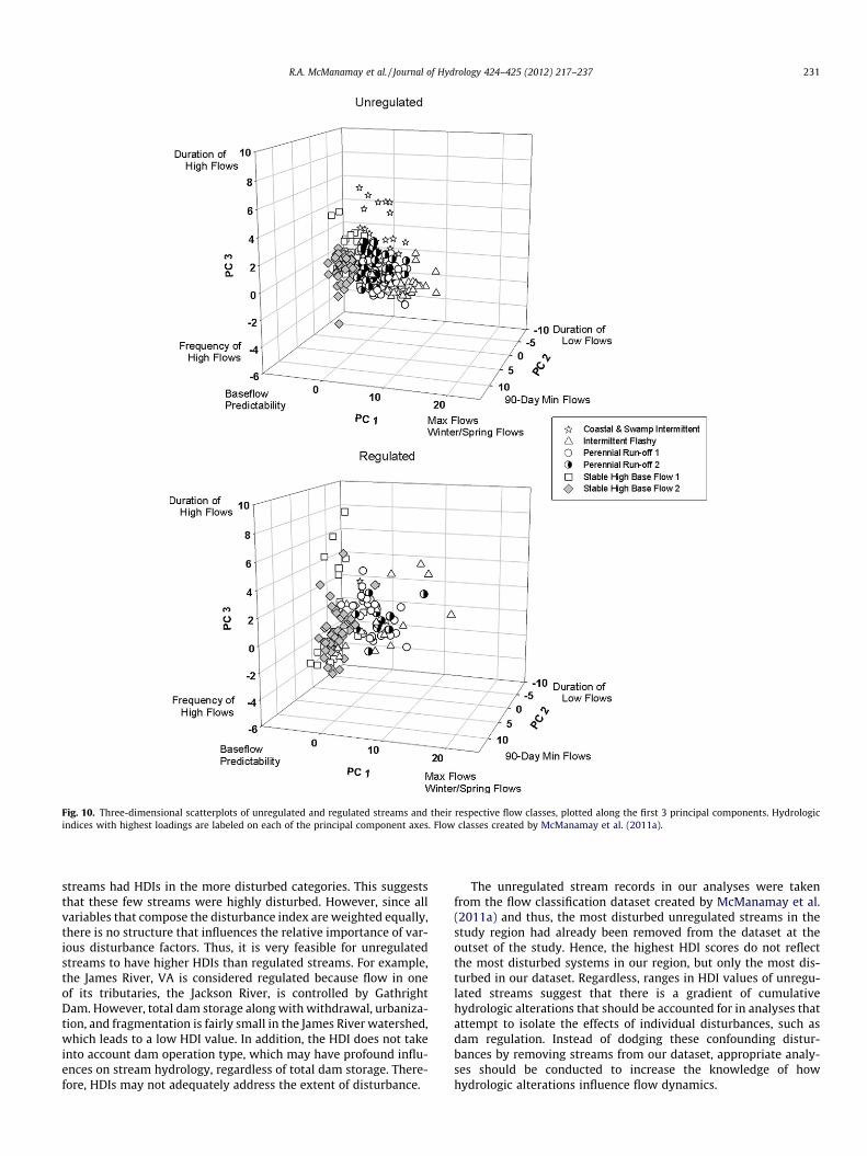
Fig. 10. Three-dimensional scatterplots of unregulated and regulated streams and their respective flow classes, plotted along the first 3 principal components. Hydrologicindices with highest loadings are labeled on each of the principal component axes. Flow classes created by McManamay et al. (2011a).
R.A. McManamay et al. / Journal of Hydrology 424–425 (2012) 217–237 231
streams had HDIs in the more disturbed categories. This suggeststhat these few streams were highly disturbed. However, since allvariables that compose the disturbance index are weighted equally,there is no structure that influences the relative importance of var-ious disturbance factors. Thus, it is very feasible for unregulatedstreams to have higher HDIs than regulated streams. For example,the James River, VA is considered regulated because flow in oneof its tributaries, the Jackson River, is controlled by GathrightDam. However, total dam storage along with withdrawal, urbaniza-tion, and fragmentation is fairly small in the James River watershed,which leads to a low HDI value. In addition, the HDI does not takeinto account dam operation type, which may have profound influ-ences on stream hydrology, regardless of total dam storage. There-fore, HDIs may not adequately address the extent of disturbance.
The unregulated stream records in our analyses were takenfrom the flow classification dataset created by McManamay et al.(2011a) and thus, the most disturbed unregulated streams in thestudy region had already been removed from the dataset at theoutset of the study. Hence, the highest HDI scores do not reflectthe most disturbed systems in our region, but only the most dis-turbed in our dataset. Regardless, ranges in HDI values of unregu-lated streams suggest that there is a gradient of cumulativehydrologic alterations that should be accounted for in analyses thatattempt to isolate the effects of individual disturbances, such asdam regulation. Instead of dodging these confounding distur-bances by removing streams from our dataset, appropriate analy-ses should be conducted to increase the knowledge of howhydrologic alterations influence flow dynamics.

Fig. 11. Three-dimensional scatterplots of principal component analyses for unregulated and regulated streams within each of the six flow classes created by McManamayet al. (2011a). Streams were plotted along the first 3 principal components. Hydrologic indices with highest loadings are labeled on each of the principal component axes.
232 R.A. McManamay et al. / Journal of Hydrology 424–425 (2012) 217–237
5.3. Hydrologic disturbance models
To isolate the effects of dam regulation, we had to control forother factors that may also explain variability in hydrologic indi-ces, such as drainage area and watershed disturbance factorsthrough general linear models. Drainage area explained 0–73% of
the variation in unregulated streams, depending on the hydrologicindex and flow class (Table 4). This suggests that our analysescould have been very biased without controlling for drainage area,since dams tend to impound larger river systems. After controllingfor drainage area, we found that the mean value of hydrologicresponse variables among flow classes spanned a large range

R.A. McManamay et al. / Journal of Hydrology 424–425 (2012) 217–237 233
compared to regulation type (Fig. 5). Flow classes represent dis-tinct hydrologic properties (Poff, 1996; McManamay et al.,2011a), but they also represent systems distinguished by differentclimate, soils, and topography (McManamay et al., 2011b). Thelarge range in variation explained by flow classes suggests thataccounting for flow class membership in analyses may controlfor the natural factors that influence hydrology. Therefore, flowclasses were used as a surrogate for geographical differencesamong basins.
The results of the MANCOVA showed that the effects of flowclass membership, dam regulation, urbanization, withdrawals,and fragmentation were all highly significant; however, dam reg-ulation had the largest effect (Table 2). Although the MANCOVAresults were informative, they did not provide specific informa-tion concerning the individual response of hydrologic variables,especially within different flow classes. Hydrologic disturbancemodels explained 0–69% (R2 adj.) of the variation in hydrologicindices for all streams depending on the individual hydrologic in-dex and flow class (Table 5). In addition, the ranges in R2 valuessuggests that some patterns in hydrologic indices are either noteasily generalized or are not influenced by our specific predictorvariables whereas other indices showed stronger patterns.Furthermore, this suggests that some prioritization can be madeconcerning which hydrologic variables to focus attention inhydrologic alteration studies. For example, Gao et al. (2009)isolated a few representative indicators out of the 32 IHAvariables that explained the majority of the variation in hydro-logic alterations.
Dam regulation explained the majority of variation in 65% ofstatistically significant models within flow classes; however,urbanization, fragmentation, and withdrawals explained themajority of variation in a substantial number of models (Table 5).Similarly, when compared to other disturbance factors, dam regu-lation had the largest and most consistent effect on flow acrossclasses (Fig. 8). However, we also found that the effects of urbani-zation may compound the effects of dam regulation while with-drawals and fragmentation tend to counter them (Fig. 8).Although dam regulation explained up to 39% of the overall varia-tion in the individual flow class models, fragmentation and urban-ization explained up to 35% and 34% of the variation in models,respectively (results not shown). Altogether this suggests thatnot accounting for these factors may have resulted in confoundedanalyses. Thus, it may be very important to isolate individual dis-turbances within basins in order to understand how each may alterflow. Despite the compounding and countering effects of other dis-turbances, we were able to isolate some general patterns in hydrol-ogy attributed to dam regulation. For example, dam regulationdecreased flow variability, 1-day maximum flows, flood intervals,and rise rates whereas the frequency of low flows and reversalsshowed increases (Fig. 8). In addition, dam storage gave very
Table 3General trends of the influence of dams on stream hydrology found in literature, across allthe direction of the influence of dams on each hydrologic variable. All variables included
Entire sample or class Decrease
Generalizations from literaturea Maximum flows, flow variability, rise/fall ratAll classes (this study) Maximum flows, flow variability, rise rate, lo
duration, flood intervalIntermittent-flashy Spring flowsPerennial run-off 1 February flow, seasonal flood predictability
Perennial run-off 2 Low pulse variability, flow predictabilityStable high baseflow 1 Winter/spring flows, flow predictabilityStable high baseflow 2 Winter/spring flows, minimum flows, baseflo
low pulse variability, flow predictability
a Richhter et al. (1996), Magilligan and Nislow (2001), Magilligan and Nislow (2005),
similar results to the regulated versus unregulated classificationand thus, could be used as a surrogate for dam regulation ingeneral.
Disturbance models showed that the magnitude and the direc-tion of the influence of dam regulation on hydrology vary quite dif-ferently depending on the individual hydrologic index and the flowclass (Fig. 6 and 7). PR1 streams and the stable high baseflowstreams showed the strongest affects of dam regulation; however,this may be associated with higher sample sizes in each of theseclasses. Across all classes, maximum flows, flow variability, riserates, low flow durations, and flood intervals generally showed de-creases whereas low-flow pulse counts, high-pulse variability, andreversals showed increases, some of which are similar to findingsin other studies (Magilligan and Nislow, 2001, 2005; Pyron andNeumann, 2008; Poff et al., 2007) (Table 3). Thus, there are somebroad generalizations that can be made concerning the influenceof dams on river systems, despite large pre-existing differences(Table 3). Typically, minimum flows show increases followingdam regulation (Magilligan and Nislow, 2001, 2005; Pyron andNeumann, 2008; Poff et al., 2007). However, we found that the ef-fect of dams on minimum flows varied depending on class (Table3). For example, IF and PR1 streams showed positive effects ofdam regulation on minimum flow. Yet, the other classes wereeither impartial or showed strong decreases in minimum flow(e.g. SBF2). Additionally, the effect of dam regulation on baseflows,predictability, and average monthly flows showed inconsistent re-sults across flow classes, but showed stronger results within flowclasses. Again, this suggests that rivers may be influenced differ-ently by dams according to their pre-existing natural flow regimes.The fact that flow regimes may be homogenized by dam regulation(Poff et al., 2007) does not insinuate that dams affect all rivers sim-ilarly. Rather, homogenization of flow regimes suggests that damsmoderate or negate the natural processes responsible for the diver-gence of flow regimes (Poff et al., 2007). For example, IF, PR1, andPR2 streams showed increases in the annual minimum whereasSBF1 and SBF2 streams show decreases. The result is that, for someindividual hydrologic indices, flows within very different river sys-tems may appear more similar following dam regulation.
Although models explained substantial variation for somehydrologic variables, the poor predictive ability of our hydrologicdisturbance models for other hydrologic variables suggests thatmodel structure may have been inappropriate given the data(i.e. non-linear relationships). For example, Carlisle et al. (2010a)built regression trees using climate, geologic, soil, topographic,and geographic variables to predict hydrologic indices across theUS. The trees were highly accurate compared to static classifica-tions, which suggests that hierarchical structure may have in-creased model predictive power. However, linear regressionmodels have been used to predict hydrologic indices and have ex-plained substantial amounts of variation in response variables in
streams found in this study, and specific to each class. Decrease and increase indicatehad a t statistics with p < 0.05.
Increase
es Minimum flows, reversalsw flow Reversals, low flow pulse counts, high pulse variability
Minimum flows, baseflow index, flow predictability, flood frequencyMinimum flows, baseflow index, fall flows, June flow, floodfrequency, date of annual maximum, flow predictabilityHigh pulse count, seasonal flood predictabilitySummer/fall flows, flood frequency
w index, High pulse count, flood frequency, seasonal flood predictability
Pyron and Neumann (2008) and Poff et al. (2007).
234 R.A. McManamay et al. / Journal of Hydrology 424–425 (2012) 217–237
various regions (DeWalle et al., 2000; Sanborn and Bledsoe, 2006;Mohamoud, 2008; Zhu and Day, 2009). Another potential sourceof unexplained variability was the exclusion of local factors (e.g.soil, climate) that may have been important in predicting hydro-logic indices. We used flow classes as a stratification to controlfor climate, geology, and topography and then developed distur-bance linear models separately for each class. Similarly, Sanbornand Bledsoe (2006) stratified basins in Colorado by major differ-ences in flow regime and geography and developed separatelinear regressions to predict streamflow metrics for each type.However, climate, geomorphology, and soil factors may exertvarious localized controls on hydrology, depending on regionalaffiliation (Mohamoud, 2008). Thus, including natural factors inhydrologic alteration models may have increased our predictiveability. One limitation, however, was that the number ofpredictors in models were limited given the sample size in eachclass.
5.4. Overall variation in flow dynamics of regulated and unregulatedstreams
The results of the PCA suggested that dam regulation pushedthe flowing environment outside the bounds of normal river func-tion rather than homogenizing river flows. Furthermore, thiswould also suggest that the cumulative effects of dams on themulti-dimensional fluvial habitats creates environments to whichendemic riverine biota are maladapted (Poff et al., 1997; Bunn andArthington, 2002). We hypothesized that in a multivariate analy-sis, such as PCA, the effects of homogenization would be mani-fested by regulated streams showing higher correlative structureand occupying a smaller multivariate space (i.e. less divergence)than their unregulated counterparts. However, we found thatunregulated streams were actually highly correlated and filled amore confined multivariate space relative to regulated streams,which occupied a larger multivariate area with more randomspread (Figs. 10 and 11). Thus, in the multivariate sense, streamhydrology does not appear to be homogenized by dams. However,this may reflect the fact that we used 38 variables in the PCArather than a fewer number of dominant hydrologic indices thatexert a larger relative influence on river function and habitats. Ifthose dominant hydrologic indices tend to be stabilized by damregulation, as in the case of maximum flows and rise rates, thenin an ecologically meaningful sense, rivers may be homogenizedby dams.
The fact that the flow regime is a multivariate term is not anew concept (Poff et al., 1997). Free-flowing streams are subjectto natural constraints in hydrology; that is, there are typicalreoccurring patterns and relationships among hydrologic vari-ables (Leopold, 1994), which lead to correlative structure. Forexample, streams characterized by intermittency will most likelyhave high daily variability, high flood frequency, and rapid riserates (Poff, 1996; McManamay et al., 2011a). In regulatedstreams, dams impose unnatural constraints on river systemsand break the typical reoccurring hydrologic pattern, which leadsto poor correlations among hydrologic variables. Thus, even ifsome hydrologic variables respond similarly to dam regulation,the fact that other variables respond differently or do not re-spond at all will cause low correlative structure. In addition,the starting point of divergence from the norm (i.e. flow class)may be far different despite a similar direction in the responseof hydrologic variables.
Similar to our evaluation of individual hydrologic indices, damregulation affected the overall variability in flow differentlydepending on flow class. Not surprisingly, different hydrologicindices had the highest loadings for different flow classes. Thus,in terms of providing environmental flow standards for altered
systems, it may be important to evaluate different subsets ofhydrologic variables that are relevant to each flow class (Oldenand Poff, 2003). Interestingly, the PCA showed that some regulatedrivers were embedded in the multivariate space of unregulated riv-ers whereas others showed extensive divergence (Fig. 11). Examin-ing the multivariate structure of flow dynamics may provide aframework to isolate systems that are the most altered, whichshould have implications for ecological relationships and manage-ment. For example, systems that show large hydrologic alterationsmay also display major shifts in fish or macroinvertebrate assem-blages (Bunn and Arthington, 2002) and losses in native fauna(Moyle and Mount, 2007).
There are a few limitations of our analyses that may have influ-enced the dispersion of streams in the PCA. One source of uncer-tainty is that the disturbances responsible for the divergence insome of the regulated streams may have been induced by otherfactors besides dam regulation. However, the range of HDI valuesindicates that regulated and unregulated streams were subject toa variety of disturbances. Furthermore, the variation in HDI valuesfor unregulated streams were higher than that of regulatedstreams. In order to account for differences in disturbances, appro-priate analyses, such as model building (this study) or basin-spe-cific historical reconstructions of stream flow (Vogl and Lopes,2009), may be needed to separate confounding effects of variouswatershed disturbances. Another potential source of dispersion inregulated streams is that some regulated streams were impoundedby more than 1 dam. However, if the homogenization-by-damsprinciple holds true, then we would expect that variability woulddecrease with consecutive impoundments. Misclassifying regu-lated streams could be an additional source of variation. However,given the accuracy rates of our predictive tools, we expectmisclassification rates to be minor. Furthermore, 32% of our regu-lated gages had pre-regulation hydrologic information that wasused in the flow classification by McManamay et al. (2011a). Thus,these regulated stream records were already assigned to correctclasses.
5.5. Potential for restoring regulated river flows
Due to the social, economic, political, and ecological complexi-ties of managing for natural flow variability in rivers with alteredhydrology, most flow rules have been limited to overly simplifiedor overly generalized standards (Arthington et al., 2006). It isnow widely accepted that sustainable water management in riversystems will require abandoning static water allocation strategiesand adopting strategies that protect the magnitude, frequency,duration, timing, and rate of change in flow (Poff et al., 1997;Arthington et al., 2006; Richter, 2010). New policies will requireestablishing socially acceptable sustainability boundaries that pro-tect the ecological integrity of river systems (Richter, 2010). Flowclassifications provide a less complex approach to managementby establishing environmental flow standards for groups ofstreams that share similar hydrology rather than managing forthe individuality of every river system. The range of variability rep-resented in flow classes should provide the structure from whichboundaries or limits to hydrologic alteration are established.According to Poff et al. (2010), influencing the societal and politicaldriven process of developing regional flow standards to protectnatural flow regimes will require developing generalized relation-ships between altered flow regimes and ecology. Our resultssuggest that rivers in different flow classes may respond differentlyto a single type of disturbance. Furthermore, we presume thatrivers within a particular flow class may also share similar ecolog-ical properties as well as similar ecological responses to alteredflow conditions (Poff et al., 2010). In summary, flow classifications,on a regional scale, should provide the baselines from which
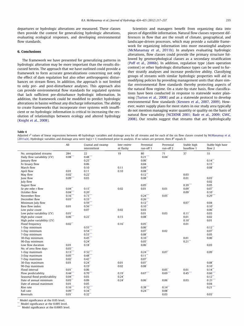
R.A. McManamay et al. / Journal of Hydrology 424–425 (2012) 217–237 235
departures or hydrologic alterations are measured. These classesthen provide the context for generalizing hydrologic alterations,evaluating ecological responses, and developing environmentalflow standards.
6. Conclusions
The framework we have presented for generalizing patterns inhydrologic alteration may be more important than the results dis-cussed herein. The approach that we have outlined could provide aframework to form accurate generalizations concerning not onlythe effect of dam regulation but also other anthropogenic distur-bances on stream flows. In addition, the approach is not limitedto only pre- and post-disturbance analyses. This approach alsocan provide environmental flow standards for regulated systemsthat lack sufficient pre-disturbance hydrologic information. Inaddition, the framework could be modified to predict hydrologicalterations in basins without any discharge information. The abilityto create frameworks that incorporate river systems with insuffi-cient or no hydrologic information is critical to increasing the res-olution of relationships between ecology and altered hydrology(Knight et al., 2008).
Table 4Adjusted r2 values of linear regressions between 40 hydrologic variables and drainage ar(2011a,b). Hydrologic variables and drainage area were log(x + 1) transformed prior to an
All Coastal and swampintermittent
Inte rmnt flash
No. unregulated streams 284 22 19Daily flow variability (CV) 0.08*** 0.48***
January flow 0.25**
Fe bruary flow 0.06March flow 0.10 0.11April flow 0.01 0.11 0.10May flow 0.02* 0.22*
June flow 0.09*** 0.03July flowAugust flowSe pte mbe r flow 0.04** 0.15* 0.02October flow 0.04*** 0.20*
November flow 0.16*** 0.73***
December flow 0.03** 0.33**
Minimum July flow 0.59***
Base flow index 0.01 0.56***
Low pulse count 0.07 0.02Low pulse variability (CV) 0.01*
High pulse count 0.06*** 0.22* 0.15High pulse variability (CV)Flood frequency 0.02** 0.16*
1-Day minimum 0.55***
3-Day minimum 0.54***
7-Day minimum 0.53***
30-Day minimum 0.45***
90-Day minimum 0.24*
Low flow duration 0.01 0.18*
No. of zero flow days 0.03**
1-Day maximum 0.13*** 0 52***
3-Day maximum 0.05*** 0.48***
7-Day maximum 0.02* 0.42**
30-Day maximum 0.01 0.24* 0.0190-Day maximum 0.19* 0.02Flood interval 0.01* 0.06Flow predictability 0.44*** 0.70*** 0.19*
Seasonal flood predictability 0.04*** 0.03 0.24*
Date of annual minimum 0.03** 0.09 0.24*
Date of annual maximum 0.01 0.05Rise rate 0.16*** 0 52***
Fall rate 0.09*** 0.34**
Reversals 0.01* 0.32**
* Model significance at the 0.05 level.** Model significance at the 0.005 level.*** Model significance at the 0.0005 level.
Scientists and managers benefit from organizing data intopieces of digestible information. Natural flow classes represent dif-ferences in flow that are the result of climate, geographical, andlandscape-driven processes, which may provide a suitable frame-work for organizing information into more meaningful analyses(McManamay et al., 2011b). In analyses evaluating hydrologicalterations, flow classes could provide the primary structure fol-lowed by geomorphological classes as a secondary stratification(Poff et al., 2006b). In addition, regulation type (dam operationcontext) or other hydrologic disturbance types can be used to fur-ther stratify analyses and increase predictive ability. Classifyinggroups of streams with similar hydrologic properties will aid inmodifying policies by providing management units that share sim-ilar environmental flow standards thereby protecting aspects ofthe natural flow regime. On a state-by-state basis, flow classifica-tions have been conducted in response to statewide water plan-ning (Turton et al., 2008) and as a statewide protocol to developenvironmental flow standards (Kennen et al., 2007, 2009). How-ever, water supply plans for most states in our study area typicallydo not mention managing water quantity or quality on the basis ofnatural flow variability (NCDENR 2001; Badr et al., 2009; GWC,2008). Our results suggest that streams that are hydrologically
ea for all streams and for each of the six flow classes created by McManamay et al.alysis. If no values are present, then R2 equals 0.
ittey
Perennialrun-off 1
Perennialrun-off 2
Stable highbaseflow 1
Stable high baseflow 2
80 71 37 550.21*** 0.04*
0.06* 0.14**
0.04 0.15**
0.09** 0.08*
0.08**
0.12** 0.030.08** 0.01 0.03*
0.020.05* 0.39*** 0.050.01 0.01 0.09* 0.07*
0.09* 0.10*
0.24*** 0.05* 0.29***
0.26***
0.12** 0.07* 0.040.10** 0.10*
0.03 0.06*
0.01 0.03 0.11* 0.030.08* 0.01 0.02
0.10* 0.010.05* 0.010.06* 0.12**
0.07* 0.02 0.07*
0.08* 0.050.10** 0.01 0.06*
0.05* 0.21**
0.06* 0.03
0.24*** 0.07* 0.09*
0.11**
0.07*
0.07* 0.08*
0.08* 0.10*
0.05* 0.01 0.14**
0.67*** 0.69*** 0.45*** 0.66***
0.12**
0.06* 0.06* 0.03 0 21***
0.040.38*** 0.14** 0.21***
0.24*** 0.08*
0.03 0.03*

236 R.A. McManamay et al. / Journal of Hydrology 424–425 (2012) 217–237
distinct will respond differently to disturbance. Thus, an obviousconclusion is that streams should be not be managed based upontheir locations with various geographic or political boundariesbut based upon similar hydrologic properties. We suggest that re-gional flow management should be based on developing naturalhydrologic baselines (e.g. flow classes) for groups of streams ratherthan region-wide water allocation policies or static minimum flowpolicies for reservoir operations. In addition, generalizing thehydrological and ecological response of rivers to disturbanceshould isolate management applications that are suitable to thedifferent needs of diverse river systems.
Overall, dam regulation exerted the strongest and most consis-tent influences on flow dynamics compared to other disturbancevariables. However, for some hydrologic indices, other distur-bances in a basin may compound or counter the influences ofdam regulation. Analyses should isolate the various contributorsto overall hydrologic alteration. Information and large datasestsconcerning hydrology and lanscape-scale variables are now morereadily available than ever (e.g. Falcone et al., 2010, Wollocket al., 2004). Thus, there is great potential to understand generalpatterns in hydrologic alterations across the landscape.
Table 5Adjusted R2 values for 40 hydrologic disturbance models for all streams and for each of theregulation, withdrawals, watershed fragmentation, and urbanization. Number of streams rexplained the most variation in each model (r = dam regulation, w = withdrawals, f = fragm
Hydrologic disturbance model All Coastal and swampintermittent
Intermitteflashy
Number of streams 401 26 30Daily flow variability (CV) 0.13*** r 0.46**
January flow 0.08*** w 0.12** f 0.26February flow 0.10*** w 0.07 f 0.29March flow 0.09*** w 0.16 f 0.28April flow 0.08*** w 0.27 f 0.27May flow 0.02* w 0.17 f 0.16June flow 0.04*** f 0.02 r 0.17July flow 0.07*** w 0.24August flow 0.07*** f 0.12September flow 0.23*** f 0.08 f 0.24October flow 0.17*** f 0.43* fNovember flow 0.08*** f 0.28 r 0.32**
Decemberflow 0.05*** w 0.33Minimum July flow 0.05*** u 0.28Base flow index 0.06*** u 0.69*
Low pulse count 0.25*** r 0.41** w 0.41Low pulse variability (C V) 0.04*** f 0.31 w 0.17High pulse count 0.10*** r 0.19 w 0.33High pulse variability (CV) 0.19*** r 0.02 f 0.50Flood frequency 0.08*** r 0.16 w 0.201-Day minimum 0.04*** u 0.51*
3-Day minimum 0.07*** u 0.627-Day minimum 0.10*** u 0.6630-Day minimum 0.15*** r 0.10 r 0.6790-Day minimum 0.15*** u 0.23 f 0.25Low flow duration 0.26*** r 0.32 r 0.34No. of zero flow days 0.07*** f 0.461-Day maximum 0.11*** r 0.423-Day maximum 0.12*** r 0.397-Day maximum 0.12*** r 0.3530-Day maximum 0.09*** w 0.14** f 0.3290-Day maximum 0.08*** w 0.15 f 0.31Flood interval 0.08*** r 0.07 r 0.13Flowpredictability 0.12*** f 0.05 w 0.59**
Seasonal flood predictability 0.06*** f 0.08 f 0.12Date of annual minimum 0.10*** r 0.29 fDate of annual maximum 0.06Rise rate 0.04*** r 0.37*
Fafl rate 0.04** f 0.11Reversals 0.26*** r 0.24* r 0.43*
* Model significance at the 0.05 level.** Model significance at the 0.005 level.*** Model significance at the 0.0005 level.
Acknowledgements
This work was funded by the Cheoah Fund Board, a multi-agencycollaboration between Alcoa Power, USDA Forest Service, US Fishand Wildlife Service, North Carolina Wildlife Resources Commis-sion, and the NC Division of Water Resources-DENR and other grantsprovided by the USDA Forest Service. We are thankful for the valu-able input from Paul Angermeier and Emmanuel Frimpong regard-ing statistical procedures and study design. We are also thankfulfor useful comments by two anonymous reviewers that improvedthis manuscript. Assistance with stream gage data compilationand management was provided by Tyler Young and Adam Hart.
Appendix A
See Table 4.
Appendix B
See Table 5.
six flow classes created by McManamay et al. (2011a,b). Models included effect of damefers to unregulated and regulated streams. Letters indicate which predictor variable
entation, u = urbanization). If no values are present, then R2 equals 0.
nt Perennialrun-off 1
Perennialrun-off 2
Stable highbaseflow 1
Stable highbaseflow 2
111 84 54 96r 0.05 r 0.07* r 0.33*** r 0.25*** ru 0.02 u 0.10 w 0.08 r 0.15 ru 0.06 r 0.07 w 0.15 r 0.20 ru 0.04 w 0.20 r 0.18 ru 0.05 f 0.13 r 0.09 ru 0.02 f 0.02 ru 0.13*** r 0.11* u 0.04 u 0.07 fw 0.07 u 0.23 w 0.18 f 0.10 wf 0.04 w 0.10 w 0.17 r 0.01 wu 0.32*** r 0.11 f 0.33 r 0.04 f
0.15 r 0.01 u 0.23 r 0.26** fu 0.20 r 0.02 r 0.24 f 0.19 wu 0.06 w 0.09 f 0.13 rr 0.09*** r 0.16 u 0.12 f 0.18 ru 0.10 r 0.06 u 0.01 r 0.18 ru 0.15 u 0.23* r 0.37*** r 0.21 rw 0.10 f 0.09 r 0.09 w 0.10 ru 0.01 f 0.09 r 0.36* w 0.12 rr 0.23*** r 0.02 r 0.43 r 0.38* rr 0.07 r 0.07 r 0.12 ru 0.14 r 0.08*** u 0.05 w 0.27 ru 0.15 r 0.09 u 0.03 w 0.21 fr 0.16 r 0.11 u 0.04 w 0.11 fu 0.21 r 0.19 u 0.16 r 0.11 fw 0.19 r 0.33 u 0.16 f 0.11 fu 0.15 u 0.23 r 0.46* r 0.23 rur 0.04 r 0.07* r 0.31*** r 0.33*** rr 0.01 r 0.04 w 0.27 r 0.29 ru 0.03 w 0.22 r 0.20 ru 0.03 w 0.11 r 0.09 ru 0.04 w 0.07 r 0.09 rr 0.13 u 0.08 r 0.16 ru 0.04*** r 0.06 r 0.30* r 0.07 ru 0.04 r 0.17 u 0.16 f
0.06 uu 0.09** r 0.03 u 0.01 fr 0.02 r 0.03 w 0.31*** r 0.22*** rr 0.09 w 0.15 w 0.03 uu 0.08*** u 0.35** r 0.50** r 0.34*** r
R.A. McManamay et al. / Journal of Hydrology 424–425 (2012) 217–237 237
Appendix A. Supplementary material
Supplementary data associated with this article can be found, inthe online version, at doi:10.1016/j.jhydrol.2012.01.003.
References
Arthington, A.H., Bunn, S.E., Poff, N.L., Naiman, R.J., 2006. The challenge of providingenvironmental flow rules to sustain river systems. Ecol. Appl. 16, 1311–1318.
Badr, A.W., Wachob, A., Gellici, J.A., 2009. South Carolina Water Plan, second ed.South Carolina Department of Natural Resources. <http://www.dnr.state.sc.us/>.
Brown, D.G., Johnson, K.M., Loveland, T.R., Theobald, D.M., 2005. Rural land-usetrends in the conterminous United States, 1950–2000. Ecol. Appl. 15, 1851–1863.
Bunn, S.E., Arthington, A.H., 2002. Basic principles and ecological consequences ofaltered flow regimes for aquatic biodiversity. Environ. Manage. 30, 492–507.
Carlisle, D.M., Falcone, J., Wolock, D.M., Meador, M.R., Norris, R.H., 2010a. Predictingthe natural flow regime: models for assessing hydrological alteration instreams. River Res. Appl. 26, 118–136.
Carlisle, D.M., Wollock, D.M., Meador, M.R., 2010b. Alteration of streamflowmagnitudes and potential ecological consequences: a multiregionalassessment. Front. Ecol. Environ. 2010. doi:10.1890/100053.
DeWalle, D.R., Swistock, B.R., Johnson, T.E., McGuire, K.J., 2000. Potential effects ofclimate change and urbanization on mean annual streamflow in the UnitedStates. Water Resour. Res. 36, 2655–2664.
Falcone, J.A., Carlisle, D.M., Wolock, D.M., Meador, M.R., 2010. GAGES: a stream gagedatabase for evaluating natural and altered flow conditions in the conterminousUnited States. Ecology, 91, 621 (Ecol. Arch. E091-045-D1).
Gao, Y.X., Vogel, R.M., Kroll, C.N., Poff, N.L., Olden, J.D., 2009. Development ofrepresentative indicators of hydrologic alteration. J. Hydrol. 374, 136–147.
Graf, W.L., 1999. Dam nation: a geographic census of American dams and theirlarge-scale hydrologic impacts. Water Resour. Res. 35, 1305–1311.
Georgia Water Council (GWC), 2008. Georgia Comprehensive State-wide WaterManagement Plan. Georgia Environmental Protection Division. <http://www.georgiawaterplanning.org/>.
Henriksen, J.A., Heasley, J., Kennen, J.G., Nieswand, S., 2006. Users’ Manual for theHydroecological Integrity Assessment Process software (Including the NewJersey Assessment Tools). US Geological Survey Report 2006-1093. <http://www.fort.usgs.gov/Resources/Research_Briefs/HIP.asp>.
Jackson, D.A., 1993. Stopping rules in principal components-analysis – a comparisonof heuristic and statistical approaches. Ecology 74, 2204–2214.
Jain, A.K., 2010. Data clustering: 50 years beyond k-means. Pattern Recogn. Lett. 31,651–666.
Jenks, G.F., 1967. The data model concept in statistical mapping. Int. Yearb. Cartogr.7, 186–190.
Kennard, M.J., Mackay, S.J., Pusey, B.J., Olden, J.D., Marsh, N., 2010a. Quantifyinguncertainty in estimation of hydrologic metrics for ecohydrological studies.River Res. Appl. 26, 137–156.
Kennard, M.J., Pusey, B.J., Olden, J.D., Mackay, S.J., Stein, J.L., Marsh, N., 2010b.Classification of natural flow regimes in Australia to support environmentalflow management. Freshw. Biol. 55, 171–193.
Kennen, J.G., Hendriksen, J.A., Nieswand, S.P., 2007. Development of theHydroecological Integrity Assessment Process for Determining EnvironmentalFlows for New Jersey Streams. US Geological Survey Scientific InvestigationsReport 2007-5206.
Kennen, J.G., Hendriksen, J.A., Heasley, J., Cade, B.S., Terrell, J.W., 2009. Applicationof the Hyroecological Integrity Assessment Process for Missouri streams. USGeological Survey Scientific Investigations Report 2009-1138.
Kenny, J.F., Barber, N.L., Hutson, S.S., Linsey, K.S., Lovelace, J.K., Maupin, M.A., 2009.Estimated Use of Water in the United States in 2005: U.S. Geological SurveyCircular 1344.
Knight, R.R., Gregory, M.B., Wales, A.K., 2008. Relating streamflow characteristics tospecialized insectivores in the Tennessee River Valley: a regional approach.Ecohydrology 1, 394–407.
Leopold, L.B., 1994. A View of the River. Harvard University Press, Cambridge, MA.Magilligan, F.J., Nislow, K.H., 2001. Long-term changes in regional hydrologic regime
following impoundment in a humid-climate watershed. J. Am. Water Resour.Assoc. 37, 1551–1569.
Magilligan, F.J., Nislow, K.H., 2005. Changes in hydrologic regime by dams.Geomorphology 71, 61–78.
Mathews, R., Richter, B.D., 2007. Application of the indicators of hydrologicalteration software in environmental flow setting. J. Am. Water Resour. Assoc.436, 1400–1413.
McManamay, R.A., Orth, D.J., Dolloff, C.A., Frimpong, E.A., 2011a. A regionalclassification of unregulated streamflows: spatial resolution and hierarchicalframeworks. River Res. Appl. doi:10.1002/rra.1493.
McManamay, R.A., Orth, D.J., Dolloff, C.A., Frimpong, E.A., 2011b. Regionalframeworks applied to hydrology: can landscape-based frameworks capturethe hydrologic variability? River Res. Appl. doi:10.1002/rra.1535.
Mohamoud, Y.M., 2008. Prediction of daily flow duration curves and streamflow forungaged catchments using regional flow duration curves. Hydrol. Sci. 53, 706–724.
Moyle, P.B., Mount, J.F., 2007. Homogenous rivers, homogenous fauna. Proc. Natl.Acad. Sci. U.S.A. 104, 5711–5712.
North Carolina Department of Environment and Natural Resources (NCDENR), 2001.North Carolina State Water Supply Plan. Division of Water Resources. <http://www.ncwater.org>.
Olden, J.D., Poff, N.L., 2003. Redundancy and the choice of hydrologic indices forcharacterizing streamflow regimes. River Res. Appl. 19, 101–121.
Olden, J.D., Kennard, M.J., Pusey, B.J., 2011. A unifying framework to hydrologicclassification with a review of methodologies and applications in ecohydrology.Ecohydrology, in press. doi:10.1002/eco.251.
Pillai, K.C., 1955. Some new test criteria in multivariate analysis. Ann. Math. Stat. 26,117–121.
Poff, N.L., 1996. A hydrogeography of unregulated streams in the United States andan examination of scale-dependence in some hydrological descriptors. Freshw.Biol. 36, 71–91.
Poff, N.L., Ward, J.V., 1989. Implications of streamflow variability and predictabilityfor lotic community structure – a regional-analysis of streamflow patterns. Can.J. Fish. Aquat. Sci. 46, 1805–1818.
Poff, N.L., Zimmerman, J.Z.H., 2010. Ecological responses to altered flow regimes: aliterature review to inform the science and management of environmentalflows. Freshw. Biol. 55, 194–205.
Poff, N.L., Allan, J.D., Bain, M.B., Karr, J.R., Prestegaard, K.L., Richter, B.D., Sparks, R.E.,Stromberg, J.C., 1997. The natural flow regime: a paradigm for riverconservation and restoration. BioScience 47, 769–784.
Poff, N.L., Bledsoe, B.P., Cuhaciyan, C.O., 2006a. Hydrologic variation with land useacross the contiguous United States: geomorphic and ecological consequencesfor stream ecosystems. Geomorphology 79, 264–285.
Poff, N.L., Olden, J.D., Pepin, D.M., Bledsoe, B.P., 2006b. Placing global stream flowvariability in geographic and geomorphic contexts. River Res. Appl. 22, 149–166.
Poff, N.L., Olden, J.D., Merritt, D.M., Pepin, D.M., 2007. Homogenization of regionalriver dynamics by dams and global biodiversity implications. Proc. Natl. Acad.Sci. U.S.A 104, 5732–5737.
Poff, N.L., Richter, B.D., Arthington, A.H., Bunn, S.E., Naiman, R.J., Kendy, E., Acreman,M., Apse, C., Bledsoe, B.P., Freeman, M.C., Henriksen, J., Jacobson, R.B., Kennen,J.G., Merritt, D.M., O’Keeffe, J.H., Olden, J.D., Rogers, K., Tharme, R.E., Warner, A.,2010. The ecological limits of hydrologic alteration (ELOHA): a new frameworkfor developing regional environmental flow standards. Freshw. Biol. 55, 147–170.
Pyron, M., Neumann, K., 2008. Hydrologic alterations in the Wabash Riverwatershed, USA. River Res. Appl. 24, 1175–1184.
Richhter, B.D., Baumgartner, J.V., Powell, J., Braun, D.P., 1996. A method for assessinghydrologic alteration within ecosystems. Cons. Biol. 10, 1163–1174.
Richter, B.D., 2010. Re-thinking environmental flows: from allocations and reservesto sustainability boundaries. River Res. Appl. 26, 1052–1063.
Sanborn, S.C., Bledsoe, B.P., 2006. Predicting streamflow regime metrics for ungagedstreams in Colorado, Washington, and Oregon. J. Hydrol. 325, 241–261.
SAS, 2008. JMP Statistics and Graphics Guide, Release 8. SAS Institute Inc, Cary, NC.Sun, G., McNulty, S.G., Myers, J.A.M., Cohen, E.C., 2008. Impacts of multiple stresses
on water demand and supply across the Southeastern United States. J. Am.Water Resour. Assoc. 44, 1441–1457.
Trush, W.J., McBain, S.M., Leopold, L.B., 2000. Attributes of an alluvial river and theirrelation to water policy and management. Proc. Nal. Acad. Sci. U.S.A. 97, 11858–11863.
Turton, D., Fisher, B., Seilheimer, T.S., Esralew, R., 2008. An Assessment ofEnvironmental Flows for Oklahoma. US Geological Survey Report 2008OK107B.
US Army Corps of Engineers (USACE), 2011. Corps Map. National Inventory of Dams.US Army Corps of Engineers. <https://nid.usace.army.mil>.
Vitousek, P.M., Mooney, H.A., Lubchenco, J., Melillo, J.M., 1997. Human dominationof Earth’s ecosystems. Science 277, 494–499.
Vogel, R.M., Wilson, I., 1996. Probability distribution of annual maximum, mean,and minimum streamflows in the United States. J. Hydrol. Eng. 1, 69–76.
Vogl, A.L., Lopes, V.L., 2009. Impacts of water resources development on flowregimes in the Brazos River. Environ. Monit. Assess. 157, 331–345.
Ward, J.V., Stanford, J.A., 1983. The serial discontinuity concept of lotic ecosystems.In: Fontaine, T.D., III, Bartell, S.M. (Eds.), The Dynamics of Lotic Ecosystems. AnnArbor Science, Ann Arbor, pp. 29–42.
Wilks, S.S., 1932. Certain generalizations in the analysis of variance. Biometrika 24,471–494.
Wollock, D.M., Winter, T.C., McMahon, G., 2004. Delineation and evaluation ofhydrologic landscape regions in the United States using geographic informationsystem tools and multivariate statistical analyses. Environ. Manage. 34, 71–88.
Zar, J.H., 1999. Biostatistical Analysis, fourth ed. Prentice Hall, NJ.Zhu, Y., Day, R.L., 2009. Regression modeling of streamflow, baseflow, and runoff
using geographic information systems. J. Environ. Manage. 90, 946–953.