journal of bene t-cost analysis … · 2015-05-08 · journal of bene t-cost analysis ... ing those...
TRANSCRIPT
Journal of Benet-Cost Analysishttp://journals.cambridge.org/BCA
Additional services for Journal of Benet-CostAnalysis:
Email alerts: Click hereSubscriptions: Click hereCommercial reprints: Click hereTerms of use : Click here
Uncertainty in the Cost-Effectiveness of FederalAir Quality Regulations
Kerry Krutilla, David H. Good and John D. Graham
Journal of Benet-Cost Analysis / Volume 6 / Issue 01 / March 2015, pp 66 - 111DOI: 10.1017/bca.2015.7, Published online: 02 April 2015
Link to this article: http://journals.cambridge.org/abstract_S219458881500007X
How to cite this article:Kerry Krutilla, David H. Good and John D. Graham (2015). Uncertainty in the Cost-Effectiveness of Federal Air Quality Regulations. Journal of Benet-Cost Analysis,6, pp 66-111 doi:10.1017/bca.2015.7
Request Permissions : Click here
Downloaded from http://journals.cambridge.org/BCA, IP address: 129.79.125.33 on 27 Apr 2015
J. Benefit Cost Anal. 2015; 6(1):66–111doi:10.1017/bca.2015.7
c© Society for Benefit-Cost Analysis, 2015
Kerry Krutilla*, David H. Good and John D. Graham
Uncertainty in the Cost-Effectiveness ofFederal Air Quality Regulations
Abstract: In this study, we conduct a cost-effectiveness analysis of nine air qualityregulations recently issued by the U.S. Environmental Protection Agency (EPA).Taking emission reductions in the Regulatory Impact Analyses (RIAs) for theseregulations as given, we independently assess uncertainty about the compliancecosts of the regulations and the lives the regulations are estimated to save. The lat-ter evaluation is based on a formal uncertainty analysis that integrates expert judg-ments about the effects of fine particle exposures on mortality risks. These expertjudgments were given in an EPA-sponsored elicitation study conducted in 2006.The integrated judgments are used to generate probability distributions for severaltypes of cost-effectiveness ratios, including the gross and net cost per life saved, netcost per life year saved, and net cost per quality-adjusted life year (QALY) gained.The results show that the cost-effectiveness ratios exhibit considerable uncertaintyindividually and also vary widely across regulations. Within a simulated 90% con-fidence interval for the gross cost per life saved, for example, there is both the pos-sibility that benefits from lifesavings alone are sufficient to cover the rules’ costsand the possibility that no lives will be saved and cost-effectiveness ratios will beinfinite. The wide ranges for the confidence intervals suggest the need for betterinformation about the effects of fine particle exposures on mortality risks.
Keywords: air quality regulation; cost-effectiveness analysis; uncertainty analysis.
1 Introduction
In this study, we conduct a cost-effectiveness analysis of recent regulations issuedby the Office of Air and Radiation of the U.S. Environmental Protection Agency(EPA). These regulations will reduce exposures to airborne concentrations of fineparticles and other pollutants, reducing the risk of morbidity and premature mortal-
*Corresponding author: Kerry Krutilla, School of Public and Environmental Affairs,Indiana University, Bloomington, IN, USA, e-mail: [email protected] H. Good: School of Public and Environmental Affairs, Indiana University,Bloomington, IN, USAJohn D. Graham: School of Public and Environmental Affairs, Indiana University,Bloomington, IN, USA
Uncertain cost-effectiveness of air regulations 67
ity, and providing other benefits, such as improved visibility. The economic effect ofsuch regulations is significant. Regulations issued exclusively by the EPA accountfor 63%–82% of the total monetized benefits of all federal regulations, and 45%–56% of their total costs, with regulations having a primary or significant goal toimprove air quality accounting for 98%–99% of these benefits (Office of Manage-ment and Budget, 2014).
The cost and consequences of regulations that reduce mortality risks, includ-ing those targeting air pollution, have drawn the attention of academic researchers,policy makers, and stakeholders.1 Two issues have been considered. The first iswhether lifesaving regulations allocate resources cost-effectively.2 A second ques-tion concerns the effects of exposures to fine particulate matter on mortality risks,and whether these uncertainties are adequately reflected in regulatory benefit esti-mates.3 Reducing exposures to fine particulate matter often account for more than90% of the monetized benefits of EPA’s air regulations (Office of Management andBudget, 2014).
The second question has been the subject of an enormous literature, the impli-cations of which will be discussed in a later section of the article that presentsan uncertainty analysis of the mortality risk reductions associated with air regula-tions.4 The first question has been addressed by a more limited literature which isuseful to review here. In this regard, a study by John Morrall computed the cost-effectiveness of 76 federal regulations promulgated from 1967 to 2001, measuredas net resource cost per statistical life saved (Morrall, 2003). The numerator of thisratio subtracts from compliance costs all of the benefits other than those related to
1 Regulations reduce the risk of premature mortality in large populations, without the affected individ-uals being known. The term “statistical lifesavings” has traditionally been used to denote this context,but usage such as “reduced mortality risk” or “avoided premature deaths” is now increasingly common.These characterizations are used interchangeably in this study. For semantic convenience, the qualifier“statistical” is also sometimes dropped from “statistical lifesavings” and “statistical lives saved,” leavingjust the terms “lives saved” and “lifesavings.” When the “statistical” qualifier is omitted, its presenceshould be regarded as implicit.2 A related discussion in the academic literature is the extent to which benefit-cost analysis is informa-tive for making judgments about risk regulation. Heinzerling and Ackerman (2002) argue against theuse of benefit-cost analysis for this purpose, while Graham (2008), Revesz and Livermore (2008), andViscusi (2005−2006) advocate for the use of benefit-cost analysis. This article adopts the conventionaleconomic evaluation perspective represented in the latter views, and in the analytical guidance offeredto agencies from the Office of Management and Budget (OMB).3 Fine particulate matter is defined as particles having diameters of 2.5 micrometers or less (“PM2.5”).Particles in this size range can penetrate deeply into the lungs and bloodstream, creating greater health
risks than larger sized particles.4 For recent research on the possible health effects of exposures to fine particulates see Krewski et al.(2009), Lepeule et al. (2012), and Fann et al. (2012a). For recent debate and discussion about the wayuncertainties about the health effects of fine particle exposures are addressed in the evaluation of airquality regulations, see Cox (2012), Fann et al. (2012b), Fraas and Lutter (2013a,b), Fann, Lamson,Anenberg, and Hubbell (2013), Smith and Gans (2014), and Fann, Lamson, Luben, and Hubbell (2015).
68 Kerry Krutilla et al.
mortality risk. Using this measure, a break-even ratio is defined at which the netresource cost of the regulation is equal to the value of a statistical life (VSL) itsaves.5 Cost-effectiveness ratios beneath this threshold will yield benefits greaterthan their costs. A “health–health” cutoff point is also identified. This is a cost-effectiveness ratio at which the regulation has no effect on aggregate mortalityrisks, owing to the opportunity cost of the resources the regulation diverts fromother risk-reducing alternatives (see Lutter, Morrall & Viscusi, 1999). Regulationswith cost-effectiveness ratios beneath this threshold will reduce mortality risks insociety, on net. It turns out that 58% of the rules had a net cost per statistical lifesaved less than the VSL, giving positive net benefits, while 65% of the rules passedthe health–health test, yielding societal mortality risk reductions, on net. There iswide variation in the cost-effectiveness ratios of the regulations, with a six order ofmagnitude difference between the minimum and maximum.
Tengs et al. (1995) conducted a cost-effectiveness analysis of 500 private andpublic interventions reducing the risk of premature mortality. They used a netresource cost measure in the numerator, but statistical life years rather than livessaved in the denominator.6 Although the cost-effectiveness metric and sample usedin Tengs et al. (1995) differed from that in Morrall (2003), the results were broadlyconsistent. Again, there were significant differences in cost-effectiveness amongdifferent interventions. In 2013 dollars, the median net cost per statistical life yearsaved was $61,981; with the median for medical interventions at $28,039 and thosefor toxin control of $4.1 million.7 These discrepancies, and those found in Morrall(2003), are likely to be partially explained by the lumpy non-continuous nature ofsome of the investment options (making it difficult to equate incremental costs atthe margin). But the magnitude of the differences are also likely to indicate signifi-cant inefficiencies in resource allocation (Tengs & Graham, 1996).
There has been limited cost-effectiveness analysis of regulations using the“quality-adjusted life year” (QALY) outcome measure commonly used in thehealth evaluation literature (Drummond, O’Brien, Stoddart & Torrance, 2005).8
5 The “value of a statistical life” (VSL) is the marginal rate of substitution between wealth and risk,and can be measured as individual willingness to pay for small reductions in one’s own mortality risksin a defined period, divided by the risk reduction.6 Life years are computed from lives saved by distributing the lives saved to the age classes in whichthey are expected to occur, and determining the expected years of life remaining – “life years” – in eachage class based on age-class specific conditional life expectancies. The life years are then aggregatedacross age classes to give the total life years associated with the lives saved.7 A number of the interventions in this study were not subsequently implemented, so the ratios includedata from some proposed-only interventions.8 The use of QALYs as an outcome measure in the environmental health context has been much debated,in part because restrictive assumptions about utility functions are needed for cost–utility analysis to beconsistent with benefit-cost analysis (see Hubbell, 2006; Haninger & Hammitt, 2011; and Hammitt,
Uncertain cost-effectiveness of air regulations 69
The QALY is based on a utility measure for morbidity outcomes that can be com-bined with mortality impacts into a single index. Over the past decade, publishedcost-effectiveness analyses in the health evaluation field using the QALY measure(known as “cost–utility” analysis) have grown rapidly (Thorat, Cangelosi & Neu-mann, 2012).9 In 2003, the OMB recommended the use of cost–utility analysisfor the assessment of federal health, environmental, and safety regulations (Officeof Management and Budget, 2003).10 In 2006 an expert panel of the Institute ofMedicine of the National Academy of Sciences was commissioned to study thefeasibility and relevance of cost-effectiveness analysis, including cost–utility anal-ysis, for the assessment of regulatory interventions (Institute of Medicine, 2006).The panel concluded that cost-effectiveness analysis was feasible and potentiallyinformative for regulatory evaluation, and the tool was illustrated in several casestudies, including an application to EPA’s off-road diesel rule (Robinson et al.,2005).11 At the same time, EPA was assessing its experience with cost–utility anal-ysis, begun in regulatory impact assessments in 2003, and studying how to adaptcost–utility analysis for the economic evaluation of air pollution regulations (U.S.EPA, 2006).12 Cost–utility analysis has also seen some limited application in theacademic literature on air pollution-reducing interventions, e.g., Cohen, Hammittand Levy (2003).
The cost-effectiveness analysis in this study extends the literature in severalways. First, and consistent with the recommendations in the report by the Insti-tute of Medicine, the analysis is based on multiple cost-effectiveness metrics. Thisframework allows an assessment of the sensitivity of results to the different mea-sures, and comparisons to other studies of federal regulations using the differentmetrics. Our study is also the first to apply cost–utility analysis to a group of fed-eral regulations.13 This extension allows a comparison of the cost-effectiveness ofthe regulatory interventions studied to those evaluated in the health literature, wherecost–utility analysis is standard practice. Third, the analysis focuses on recent airregulations. This application is particularly policy relevant given the cost and con-sequences of these regulations. Finally, because there are significant uncertaintiesassociated with federal regulatory interventions (see Krupnick et al., 2006), and
2013). We use cost–utility analysis in this study to see how air regulations will compare with otherpublic and private health care interventions that are based on the method.9 See the Cost-Effectiveness Registry at https://research.tufts-nemc.org/cear4/Default.aspx.10 Circular A-4 is the guidance document making this recommendation. It is the most recent OMB cir-cular providing analytic guidance to agencies for preparing economic evaluations of federal regulations.11 The recommendations of the Institute of Medicine report were never formally adopted by the OMB,and in some cases differ from the guidance in Circular A-4.12 EPA has not performed a regulatory cost–utility analysis since 2008.13 As noted, previous cost–utility analyses of federal regulations have been based on individual casestudies.

70 Kerry Krutilla et al.
in particular, regulations to reduce air pollution exposures, our study considers themajor uncertainties in the analysis and conducts a formal uncertainty analysis ofthe concentration–response relationship between fine particle exposures and mor-tality risks. This formal analysis integrates the expert judgments derived from anelicitation study to compute 90% confidence intervals for the statistical lives thatthe regulations are expected to save. A 90% confidence interval is then computedfor all of the cost-effectiveness measures for each of the regulations in the study.
We begin in the next section with a description of the criteria used to selectthe regulations, and offer some perspective about their characteristics and the reg-ulatory program that includes them. The following section describes the data andmethods used to construct the cost-effectiveness ratios. The results of the analysisare then presented, followed by a discussion of the methodology implications andsuggestions for future research.
2 Sample selection and characteristics
This section describes the criteria used to select the rules in the study, and thendescribes some of their characteristics. We also report the range of estimated statis-tical lifesavings for each of the rules based on estimates for relative risk reductioncommonly used in the Regulatory Impact Analyses (RIAs) of the regulations.14
We also indicate cost-effectiveness ratios, defined as gross compliance costs perlife saved, that correspond to these estimates. In combination, this information pro-vides the context for understanding the air quality regulations in the study and theircosts and effects as the EPA estimates them. This information provides the point ofdeparture for the analysis that follows.
2.1 Sample selection
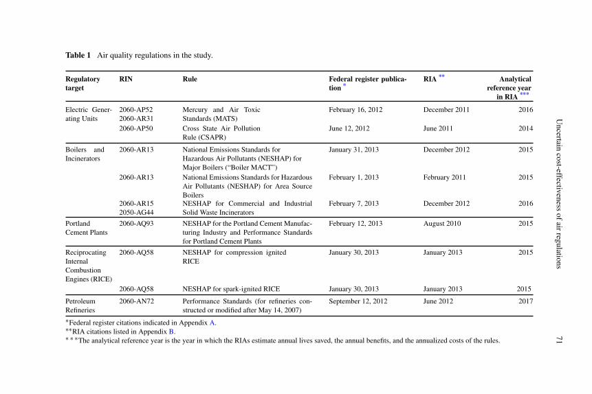
The analysis is based on a sample of EPA rules that meet two criteria. Rules hadto target stationary source emitters, and have promulgation dates between 2011and 2013. Additionally, rules had to be deemed “significant,” and have a RIA com-pleted sometime from August 2010 to December 2013. Table 1 shows the completelist of the rules included in the study.
14 “Regulatory Impact Analysis” is the terminology used to describe the benefit-cost analysis that theOMB requires for “significant regulations.” “Significant regulations” are usually those that have anannual impact of at least $100 million – either on the cost or benefit side.
Uncertain
cost-effectivenessofairregulations
71
Table 1 Air quality regulations in the study.
Regulatorytarget
RIN Rule Federal register publica-tion *
RIA ** Analyticalreference year
in RIA ***
Electric Gener-ating Units
2060-AP522060-AR31
Mercury and Air ToxicStandards (MATS)
February 16, 2012 December 2011 2016
2060-AP50 Cross State Air PollutionRule (CSAPR)
June 12, 2012 June 2011 2014
Boilers andIncinerators
2060-AR13 National Emissions Standards forHazardous Air Pollutants (NESHAP) forMajor Boilers (“Boiler MACT”)
January 31, 2013 December 2012 2015
2060-AR13 National Emissions Standards for HazardousAir Pollutants (NESHAP) for Area SourceBoilers
February 1, 2013 February 2011 2015
2060-AR152050-AG44
NESHAP for Commercial and IndustrialSolid Waste Incinerators
February 7, 2013 December 2012 2016
PortlandCement Plants
2060-AQ93 NESHAP for the Portland Cement Manufac-turing Industry and Performance Standardsfor Portland Cement Plants
February 12, 2013 August 2010 2015
ReciprocatingInternalCombustionEngines (RICE)
2060-AQ58 NESHAP for compression ignitedRICE
January 30, 2013 January 2013 2015
2060-AQ58 NESHAP for spark-ignited RICE January 30, 2013 January 2013 2015
PetroleumRefineries
2060-AN72 Performance Standards (for refineries con-structed or modified after May 14, 2007)
September 12, 2012 June 2012 2017
∗Federal register citations indicated in Appendix A.∗∗RIA citations listed in Appendix B.∗ ∗ ∗The analytical reference year is the year in which the RIAs estimate annual lives saved, the annual benefits, and the annualized costs of the rules.
72 Kerry Krutilla et al.
The time period was chosen for two reasons. First, the analysis is based onsecondary sources, and most significantly, on the RIAs themselves. The methods forpreparing RIAs continue to evolve, so basing the analysis on the relatively recentperiod offers a sample of RIAs reflecting reasonably current practices. Secondly,as Table 1 shows, this time frame coincides with a period of significant regulatoryactivity. This rulemaking reflects the somewhat fortuitous confluence of a seriesof administrative reconsiderations and legal actions largely resolving a backlog ofcontested and delayed rulemakings dating back over several administrations. Theserulemakings principally, though not exclusively, regulate the emission of hazardousair pollutants (HAPs).15
The National Ambient Air Quality Standards (NAAQS) for fine particulatematter is a notable exclusion from our study. Characteristics of NAAQS limit theusefulness of their cost estimates for comparative analysis. States have the flexibil-ity to choose different compliance strategies in multiple sectors to attain ambientstandards, and this flexibility reduces the predictability of future costs. The RIA forthe NAAQS for particulate matter describes the situation as follows:
The setting of a NAAQS does not compel specific pollution reductions andas such does not directly result in costs and benefits. For this reason, NAAQSRIAs are merely illustrative. The NAAQS RIAs illustrate the potential costsand benefits of additional steps States could take to attain a revised air qualitystandard nationwide beyond the rules already on the books (U.S. EPA, 2012,pdf pp. 36).16
2.2 Characteristics of air regulations17
The rules in this study require national emission standards for hazardous air pol-lutants (NESHAPs) with just two exceptions: the regulation targeting petroleumrefineries, and the Cross State Air Pollution Rule (CSAPR). New Source Perfor-mance Standards (NSPS) for the conventional criteria pollutants18 are also requiredin the rulemakings with just two exceptions: the CSAPR and the rule that reduceshazardous pollutants from large boilers, known as the “Boiler MACT.” In short,
15 Minor administrative reconsiderations and proposed changes have continued beyond the time frameillustrated in Table 1, and additional legal actions are likely.16 Given this uncertainty about costs, NAAQS are also excluded from the EPA’s ongoing retrospectivestudies of major rules (see Kopits et al., 2014).17 Unless otherwise indicated, the Federal Register notices indicated in Appendix A and the RIAs listedin Appendix B provide the information and data for this section.18 The “criteria pollutants” are the standard pollutants that are regulated in EPA regulations, i.e., ozone,particulate matter, carbon monoxide, nitrogen oxides, sulfur dioxide, lead.
Uncertain cost-effectiveness of air regulations 73
NESHAPs in conjunction with NSPS is the modal regulatory approach for thegroup of regulations in the study.19
The regulations target different sources of emissions (see Table 1). The strin-gency and scope of the regulations differs for these sources, reflecting differences inthe size of regulated combustion units and the fuels they use. In general, the CleanAir Act requires major sources of hazardous air pollutants – boilers or processheaters used in electric generating units or in heavy industry – to install “MaximumAchievable Control Technology” (MACT).20 Smaller boilers or sources defined as“area” sources, (for example, those used to provide heat in commercial establish-ments, schools, and hospitals), face less stringent standards consistent with the useof “Generally Available Control Technology” (GACT). Energy efficiency assess-ments and regular maintenance scheduling are the kinds of actions that might betaken to meet this category of standards.
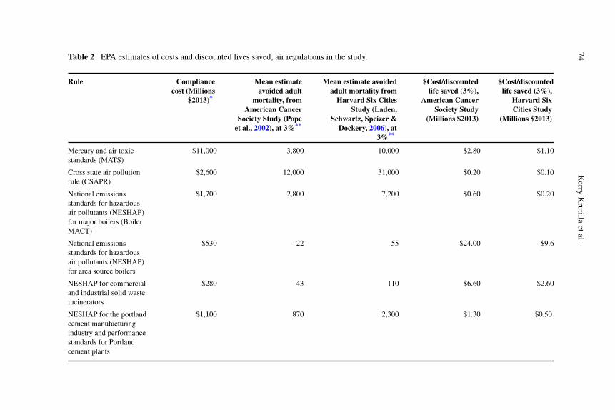
Given this regulatory framework, the rulemakings targeting the utility sectorare the most costly and are estimated to save the most lives, with Mercury and AirToxic Standards (MATS) the most costly rule in the study. Indeed, the MATS isone of the most costly rules that the EPA has ever issued, having estimated com-pliance costs of around $11 billion, or 60% of the total costs of all of the rulesin our study. The EPA also estimates that the controls installed to reduce emis-sions from utility generators will save between about 3,800 and 10,000 statisticallives annually, discounted at 3% (see Table 2). These control devices reduce fineparticles as a side effect, and it is the effects of reducing fine particles that giverise to these estimates. The figures shown are from the coefficient estimates fromreducing fine particles from two cohort-based epidemiological studies: the Ameri-can Cancer Society Study and the Harvard Six Cities Study. These studies, whichprovide updated relative risk estimates with the passage of time, give the benchmarkestimates for reduced mortality risks for all air regulations from the EPA.21
19 The Clean Air Act specifies a 3-year timetable for regulated sources to come into compliance withstandards for hazardous pollutants, and allows states and local permitting authorities to grant up toan additional year on a case by case basis. Administrative reconsiderations by EPA can restart thistimetable, and legal actions often delay the implementation schedule. As of the time of this writing, thecompliance timetable for the standards for hazardous pollutants seems likely to occur sometime in the2015–2018 period.20 Maximum Achievable Control Technology (MACT) for hazardous air pollutants has a statutorydefinition under Section 112(d) of the Clean Air Act. For example, MACT for new sources is defined asa level of control at least as stringent as that achieved by the best controlled similar source.21 These epidemiological studies follow the health status of a cohort of individuals though time, andstatistically relate the cohort’s health status to fine particle exposures and covariates. Pope et al. (2002)gives the estimates for the American Cancer Society Study shown in Table 2, while Laden et al. (2006)gives the estimates shown for the Harvard Six Cities Study. To provide additional perspective, EPA alsouses an expert elicitation study giving twelve expert opinions on the mortality effects of fine particleexposures. We discuss the cohort studies and expert elicitations further in Section 3.2.
74K
erryK
rutillaetal.
Table 2 EPA estimates of costs and discounted lives saved, air regulations in the study.
Rule Compliancecost (Millions
$2013)*
Mean estimateavoided adult
mortality, fromAmerican Cancer
Society Study (Popeet al., 2002), at 3%**
Mean estimate avoidedadult mortality from
Harvard Six CitiesStudy (Laden,
Schwartz, Speizer &Dockery, 2006), at
3%**
$Cost/discountedlife saved (3%),
American CancerSociety Study
(Millions $2013)
$Cost/discountedlife saved (3%),
Harvard SixCities Study
(Millions $2013)
Mercury and air toxicstandards (MATS)
$11,000 3,800 10,000 $2.80 $1.10
Cross state air pollutionrule (CSAPR)
$2,600 12,000 31,000 $0.20 $0.10
National emissionsstandards for hazardousair pollutants (NESHAP)for major boilers (BoilerMACT)
$1,700 2,800 7,200 $0.60 $0.20
National emissionsstandards for hazardousair pollutants (NESHAP)for area source boilers
$530 22 55 $24.00 $9.6
NESHAP for commercialand industrial solid wasteincinerators
$280 43 110 $6.60 $2.60
NESHAP for the portlandcement manufacturingindustry and performancestandards for Portlandcement plants
$1,100 870 2,300 $1.30 $0.50

Uncertain
cost-effectivenessofairregulations
75
Table 2 (Continued).
Rule Compliancecost (Millions
$2013)*
Mean estimateavoided adult
mortality, fromAmerican Cancer
Society Study (Popeet al., 2002), at 3%**
Mean estimate avoidedadult mortality from
Harvard Six CitiesStudy (Laden,
Schwartz, Speizer &Dockery, 2006), at
3%**
$Cost/discountedlife saved (3%),
American CancerSociety Study
(Millions $2013)
$Cost/discountedlife saved (3%),
Harvard SixCities Study
(Millions $2013)
NESHAP for compressionignited reciprocatinginternal combustionengines (CIRICE)
$390 77 200 $5.10 $2.00
NESHAP forspark-ignitedreciprocating internalcombustion engines(SIRICE)
$120 6 16 $19.00 $7.40
New source performancestandards (NSPS) forpetroleum refineries
$110 24 60 $4.60 $1.80
Totals*** $18,000 19,000 51,000 $0.90 $0.30
All estimates in table rounded to two significant figures.∗Subtracts out energy savings, with the exception of the Petroleum Refinery Rule. Energy savings for the petroleum refinery rule are larger than the rule’scompliance costs.∗∗EPA analyses assume that lifesavings are distributed in the periods following the implementation of the regulation according to a “cessation lag.” The discountfactor used to convert these future distributed lifesavings into a present value at a 3% discount rate (used here for illustrative purposes) is 0.9061. For the 7%discount rate, the factor is 0.8160. Multiplying the ratios in the table by 1.1036 will convert them to costs per undiscounted lives saved. Multiplying the ratios by0.9006 will give cost per discounted lives saved at 7%.∗ ∗ ∗Totals may not equal summations due to rounding.

76 Kerry Krutilla et al.
The CSAPR is the other rule that targets utilities. This rulemaking replacesthe Clean State Air Pollution Rule (CAIR), regulating the cross state transport ofozone and fine particle precursors (SOx and NOx ) from electric generating unitsin 28 states. The CSAPR costs in the neighborhood of $2.6 billion per year and,according to the benchmark EPA estimates, saves 12,000 to 31,000 lives annuallyfrom reducing fine particle exposures (see Table 2). These estimates of discountedlives saved are three times larger than those for the MATS, and constitute 60% ofthe total estimated lives saved for all of the rules in the study.
Rules regulating major boilers (The Boiler MACT) and portland cement plantseach cost over a one billion annually and save lives from the reduction of fine parti-cles (again discounted at 3%) from around 2,800 to 7,200 (in the case of the BoilerMACT) and 870 to 2,300 (for the portland cement plants). The Boiler MACT tar-gets larger industrial boilers, while the Portland Cement Rule regulates approxi-mately 158 kilns at 100 facilities.
The regulation targeting hazardous pollutants from solid waste incineratorscosts around $280 million per year, and is estimated by EPA to save 43–110 livesannually. The remaining rules target smaller sources, with lower costs and lifesav-ing effects. They include a regulation targeting smaller “area source” boilers ofthe type that provide heat in commercial establishments, and the two rules regulat-ing stationary reciprocating internal combustion engines (RICE). These engines areused to power pumps and compressors, and also to power backup generators.22
The final rule specifies NSPS for NOx emitted from process heaters in refiner-ies, and provides a flare management and monitoring plan designed to reducehydrogen sulfide emissions. This is the smallest rule in the study, with an annualcompliance cost of around $110 million, and lifesavings from 24 to 60 per year.23
Table 2 combines the cost and lifesaving estimates indicated into cost-effectiveness ratios (columns (4) and (5)). These figures can be compared to theVSL for the analytical reference year of the rules. These VSLs range between $9.0
22 Compression-ignited internal reciprocating combustion engines (CIRICE) use diesel as a fuel, whilespark-ignited reciprocating internal combustion engines (SIRICE) are fueled with gasoline or naturalgas.23 The small scale of this rule is partially an artifact of the way it is evaluated. The analysis is based onthe costs and effects of compliance of new sources in the analytical reference year 2017. An alternativeapproach would be to wait until refinery stock fully turns over, and to analyze the costs and effects ofcompliance to the NSPS by the entire industry. (This approach was used in the analysis of joint DOT–EPA rule promulgated in 2011 regulating CO2 emissions and energy consumption in medium and heavyduty trucks.) While these different analytical methods will affect costs, lives saved estimates, and netbenefits, they do not necessarily affect cost-effectiveness (or benefit-cost) ratios. Assuming that effectsare proportional to market penetration, the scale difference between partial and total industry compliance– and the temporal differences involved, as reflected in discounting – will divide out in the ratio formats.

Uncertain cost-effectiveness of air regulations 77
and $10.0 million in $2013.24 Thus, the gross compliance cost per discounted sta-tistical life saved is always less than the VSL for all of the rules in the study buttwo: the rule regulating Area Source Boilers, and the rule regulating Spark-IgnitedReciprocating Internal Combustion Engines (SIRICE). This implies that, with theexception of these two rules, the benefits of reducing fine particles, estimated fromeither of the cohort epidemiological studies represented in Table 2, are large enoughto cover compliance costs without considering any other benefits.
In sum, recent regulations to reduce the emission of hazardous air pollutants,as well as the criteria pollutants, cost around $18 billion per year in aggregate.25
Using the estimation methods and data in EPA’s regulatory impact assessments, themean lifesaving estimates for these rules in combination are over 20,000 to over55,000 lives per year, discounted at 3%. The benefit estimates associated with theselifesavings are larger than the compliance cost of the regulations for all of the rulesbut two.
3 Methods and data
This section describes the methods and information sources underlying the sev-eral cost-effectiveness metrics used in the study. We first consider the compli-ance costs of the rules, before turning to the uncertainty analysis of the lifesav-ings resulting from the regulations. Next we consider the sources and methodsfor computing net cost numerators, and then turn to an explanation of two addi-tional denominators: life years and QALYs. In combination, this development pro-vides the necessary information for computing probability distributions for thecost-effectiveness metrics.
There are many uncertainties associated with regulatory impact evaluation (seeKrupnick et al., 2006). While it is not possible to address them fully in this analysis,it is important to consider the bigger picture briefly to provide some perspectiveon the scope of our study. One key uncertainty is the emissions baseline. Futureemissions will be influenced by difficult-to-anticipate market conditions, includ-ing changes in the price of fuel and other inputs, rates of economic growth, and
24 The VSLs are based on the mean of the VSLs in 26 labor market and contingent valuation studiesconducted form 1974 to 1991. The value is $6.3 million ($2000). This figure is adjusted for incomegrowth to the analytical reference year, and then converted into $2013.25 This aggregate figure must be viewed as an approximate ballpark because it does not adjust fordifferences in the timing associated with the different analytical reference years in which the annualcosts are computed. The annual OMB reports to Congress on the benefits and costs of federal regulationsdo not make this adjustment either. If the analytical reference years are significantly different, combiningcosts and benefits from different years could lead to significant biases.

78 Kerry Krutilla et al.
technology trends. The estimation of emissions reductions that the regulation bringsabout also has uncertainties. The degree of compliance and the scope of the rule’simpact may not be known with certainty, and rulemaking delays and reconsidera-tions often end up changing the structure of the rule. Uncertainties in the emissionsbaseline and the effect of the regulation will affect both compliance costs and mor-tality risks; hence, both the numerator and denominators of the cost-effectivenessratios.26
Modeling the chemical transport and dispersion processes that translate emis-sion reductions into local concentration changes also has uncertainties. Air qualitymodels are subject to extensive validation tests (see Fann et al., 2012a), but atmo-spheric chemistry is complex. Recent research, for example, has found that inter-actions between NOx emissions and ozone and ammonia can give non-convexitiesin the formation of ozone and fine particulates – resulting in negative damages insome urban locations from increased nitrogen oxide emissions (Fraas & Lutter,2011, 2012).
Once the effects of emissions changes on concentrations have been estimated,the concentration changes are mapped to demographic characteristics at partic-ular locations, and concentration–response models are used to estimate healtheffects. There are likely to be uncertainties in future demographic conditions, butthe main uncertainty discussed in the literature concerns concentration–responsemodeling.
To make the analysis tractable, we take the reductions in emissions and expo-sure risks represented in the RIAs as given, abstracting from many of the uncer-tainties just described. This approach has the important implication that uncer-tainties about costs and lives saved can be treated independently, and channelsthe uncertainty analysis into particular areas. On the cost side, the analysis hasto focus on uncertainties around the compliance cost per emission or exposurerisk reduced, or “unit cost” as described in the literature on retrospective eval-uation (Harrington, Morgenstern & Nelson, 2000; Kopits et al., 2014). In termsof outcomes, the assumption that exposures can be taken as given implies thatuncertainty about the mortality risks per unit of exposure reduction is the rel-evant issue. We abstract from possibly relevant demographic uncertainties, andfocus on the concentration–response relationship. We now turn to the estimationof unit costs and the concentration–response relationship between exposures andmortality risks.
26 See “Special Issue: Retrospective Analysis of the Costs of EPA Regulations,” Journal of Benefit-Cost Analysis, 5, 2 (2014) for the way these uncertainties can cause ex post cost estimates to differ fromex ante estimates.

Uncertain cost-effectiveness of air regulations 79
3.1 Uncertainty in unit compliance costs27
There are significant uncertainties associated with regulatory cost estimation.Owingto the difficulty in formally modeling cost distributions, however, we chose not toconduct a formal uncertainty analysis. Rather, we use the cost estimates in the RIAsas the basis for the cost-effectiveness measures, while providing some qualitativeperspective about them.
It is important to recognize two categories of uncertainties around compliancecosts. The first is uncertainty about compliance strategies, engineering cost compo-nents, or market conditions which are known to analysts, and therefore, are mea-sured and represented in the RIAs. Initial assumptions about these factors oftenprove to be in error, and are reported in retrospective evaluations. As an exam-ple, initial assumptions about per unit compliance costs for the 1998 LocomotiveEmissions Standard were found to be half of what the cost turned out to be, dueto inaccurate assumptions about the usage rates of different control strategies, andrising fuel prices (Kopits, 2014). On the other hand, ex ante estimates of compli-ance costs for the “Cluster Rule” were subsequently found to be 30%–100% higherthan actual costs (Morgan, Pasurka & Shadbegian, 2014).28 Cleaner technology andflexible compliance options reduced costs beneath the level initially expected.
Another uncertainty concerns cost categories not generally recognized in theRIAs. Research in the energy conservation literature offers relevant insight. Individ-uals often do not undertake energy conservation investments that an outside assess-ment based on engineering cost estimates would show to be profitable (Gillingham& Palmer, 2014), suggesting that the engineering cost estimates are leaving out rel-evant information. In fact, this context arises in our study: the energy savings asso-ciated with the NSPS for petroleum refineries alone are larger than the regulatorycompliance costs. A reason that compliance is not voluntary, given this fact, couldbe unrecognized transaction costs arising from organizational or managerial con-straints, information barriers, or administrative burdens (Krutilla & Krause, 2011;Martin, Muuls, de Preux & Wagner, 2010). Not being identified in the RIAs, uncer-tainties about these types of costs will not be picked up in retrospective evaluations.
We briefly consider uncertainties of one or both of these types for the following:compliance strategies, engineering costs, the regulatory implementation scheduleand cost allocation, political transaction costs, and modeling frameworks.
27 The term “compliance cost,” as used in this study, denotes either engineering or partial equilibriumcost estimates. This usage differs than that in EPA documents. EPA uses the term “social cost” to referto costs that are estimated through multi-market modeling, and reserves the term “compliance costs” forengineering costs (see U.S. EPA, 2014).28 The “Cluster Rule” is a combined rulemaking that integrated water and air pollution control in thepulp and paper industry. It was promulgated on April 15, 1998.

80 Kerry Krutilla et al.
3.1.1 Compliance strategies
Firms have choices about compliance options, and this flexibility reduces the cer-tainty of unit cost estimations. The fact that compliance takes place over time addsuncertainty, as market conditions and technology that affect the relative cost of dif-ferent compliance alternatives change over time. The recent declines in natural gasprices, for example, have encouraged significantly more fuel switching to naturalgas in the utility sector than initially anticipated (Burtraw, Palmer, Paul & Woer-man, 2012).
Compliance options are greatest for incentive-based instruments, like tradablepermits, and as noted previously, for ambient standards. But even for performancestandards based on technology benchmarks, firms have significant compliance flex-ibility. To comply with MACT-based standards prescribed in the MATS, for exam-ple, firms can retrofit pollution controls, switch from coal to natural gas at existinggenerating units, or accelerate the retirement of coal-fired units and the planningfor new plant constructions. To the extent that these compliance options cannot befully anticipated, ex post compliance costs are likely to be different than the initialcost estimates in the RIAs (McGarity & Ruttenberg, 2001; McCarthy & Copeland,2011; McCarthy, 2012).
3.1.2 Engineering costs
If firms choose to install pollution controls, uncertainties about control costs becomerelevant for cost estimation. EPA must sometimes choose between higher estimatesmade by the regulated industry and lower cost estimates submitted by the suppliersof equipment and other inputs to the regulated industry. Unit charges are includedin EPA’s cost estimation manual, which indicates that cost estimates are accuratewithin ±30% (U.S. EPA, 2002). Assuming that estimation errors are randomlydistributed, total industry compliance cost estimates should be relatively accurate.However, EPA’s cost manual is significantly out of date. In response to the 2014Omnibus Bill, the manual is being revised over the next three years to reflect theevolution of materials prices, the component costs of pollution control systems, andthe price of labor.29
Installed costs must also be considered, and may not be fully reflected in com-pliance cost estimates in the RIAs. The enactment of the multiple overlapping rulesthat has recently taken place can make retrofitting additional pollution controls rel-atively difficult (Chicanowicz, 2011). On the other hand, compliance with multi-ple rules might also present opportunities for scale economies that would lowerunit costs.
29 See http://www.epa.gov/ttncatc1/products.html#cccinfo.
Uncertain cost-effectiveness of air regulations 81
3.1.3 Regulatory timing and cost allocation
All of the rules in the study have faced implementation delays, due to administra-tive reconsiderations and/or legal actions. Such delays can increase unit costs byaltering the timing of capital investments. Interrupted implementation also makes itdifficult to accurately discount the temporal path of investment, and to allocate costsand effects across rulemaking phases. The CSAPR provides a notable example. In2008, the District of Columbia Circuit Court of Appeals vacated CSAPR’s prede-cessor, the Clean Air Interstate Rule (CAIR), but the ruling allowed EPA to admin-ister the CAIR pending future regulation. By EPA estimates, industry incurred $1.6billion in annual costs to comply with the CAIR by the end of 2011. The replace-ment of the CAIR with the CSAPR added another $0.8 billion in compliance costs.EPA’s RIA uses the $0.8 billion cost figure, but includes the lifesaving estimatesfrom the incremental change in emissions from the 2005 emissions baseline. Incontrast, the 2012 OMB report to Congress included 30% of the total benefits inthe RIA for the CSAPR, an amount estimated to correspond with the incrementalregulation of the CSAPR beyond the CAIR rule it replaced (Office of Managementand Budget, 2012). Our study takes a third approach: both the lifesaving estimatesand the compliance costs are taken as the difference between the 2005 baseline and2013 analytical reference year.
3.1.4 Political costs
Contested regulatory implementation imposes resource costs that stakeholdersincur to try to influence outcomes. These costs are not included in conventionaleconomic cost estimates of regulatory actions, but can be tractably modeled andreflected in a modified benefit-cost standard that incorporates lobbying costs andregulatory uncertainty (Krutilla & Alexeev, 2012). The presence of transfer pay-ments, such as pollution taxes or subsidies, also influences lobbying costs andregulatory outcomes (Krutilla & Alexeev, 2014). Lobbying costs over policies withthe rights structure of regulatory standards can amount to as much as 68% of totalcompliance costs.
3.1.5 Modeling methods
Engineering cost estimation and partial equilibrium modeling are the methods usedto determine compliance costs in the RIAs in our study. Economists often makearguments for general equilibrium modeling, or dynamic market models, to better
82 Kerry Krutilla et al.
reflect the market adjustments associated with rulemakings. A well-known dynamicgeneral equilibrium assessment of the Clean Water Act found that social cost esti-mates could be higher or lower than engineering cost estimates (Hazilla & Kopp,1990). A recent dynamic econometric model of the effects of regulating hazardouspollutants in the portland cement industry found that social costs were significantlyhigher than engineering cost estimates (Ryan, 2012).30 A caveat is that the welfareeffects in these models are driven by adjustments in input usage, output, and con-sumption – owing to changes in the equilibria in factor and commodity markets thatthe regulation brings about. In both the models mentioned, for example, prices rise,and output and consumption drop. These market responses can cause emissions todrop; thus, increasing benefits. Without holding the benefit side constant, it is hardto cleanly attribute the welfare effects demonstrated in these models to the cost sideof the equation.
3.1.6 Conclusions
There are a number of factors that can cause realized unit compliance costs to varyfrom the estimates given in the RIAs, and the difference between initial estimatesand realized costs can be significant. It is not uncommon for retrospective eval-uations to find unit costs to be less than 50% to more than double the estimatesin RIAs. Although the retrospective evaluation literature is spotty, there does notseem to be a directional bias in unit cost estimates (Harrington et al., 2000; Kopitset al., 2014). However, transactions costs will impose a downward bias to unit costestimates in the RIAs, and are not measured in retrospective evaluations. The sig-nificance of these costs in the measurement of regulatory opportunity costs hasreceived only limited research.
3.2 Lives saved and uncertainty analysis
The core of EPA’s analysis of mortality risks is based on two families of cohort stud-ies. The first, using the ACS’s Cancer Prevention Study II cohort (“ACS Study”)involves approximately 500,000 adults. The second, the Harvard Six Cities Study(“SCS study”), develops its own cohort involving a little over 8,000 adults.31 Both
30 This result is also shown in static partial equilibrium models of concentrated industries, owing to thewedge between marginal values and costs (see RIA in Appendix B for Portland Cement).31 The family of studies from the ACS cohort include Pope et al., 1995, 2002; Krewski et al., 2009.The SCS cohort studies include Dockery et al., 1993; Laden et al., 2006; Lepeule et al., 2012.
Uncertain cost-effectiveness of air regulations 83
the ACS and the SCS studies follow individuals over time, estimating the relativerisk of dying prematurely based on a Cox proportional hazards model. Both theinitial ACS and SCS studies are regarded as being well done but rely on somewhatdifferent variation in fine particulate concentrations to identify their estimates.
The 2002 National Academies’ National Research Council (NRC) review ofEPA’s uncertainty analysis recommended, among other things, that the EPA includeexpert judgment about the state of knowledge in its analysis (NRC, 2002). Otherapproaches to synthesize the state of knowledge include either meta-analysis ofstudies or integrated exposure response assessment (see for example, Fann, Gilmore& Walker, 2013). Recent research by Smith and Gans (2014) and Fraas and Lutter(2013a) suggests that EPA focuses only on aleatory uncertainty and should do moreto address epistemic uncertainty. The debate and following comments (Fann, Lam-son, Anenberg, and Hubbell 2013; Fraas & Lutter, 2013b; Fann, Lamson, Luben &Hubbell, 2015) suggest that the issue remains controversial.32
One way to address epistemic uncertainty is with expert elicitations. In 2006EPA conducted an expert elicitation study on the mortality risks associated withexposure to fine particulates (Industrial Economics, Inc., 2006; Roman et al.,2008).33 The central values of the benefit estimates that follow from these expertjudgments are reported in every RIA. This expert elicitation study could alsobe used to address epistemic uncertainties about impacts for the concentration–response functions, including uncertainties about causality; uncertainties aboutthresholds or nonlinearity in the concentration–response function; and uncertaintiesabout differential toxicity of the ambient mix of fine particulate constituents. In ourstudy, we use expert elicitation studies to address the first two of these uncertain-ties. Assessment of the third uncertainty requires speciation of the fine particulatemix and source attribution of emissions and is beyond the scope of this article. Theeffects of differential toxicity of particles are not a small uncertainty and have beendiscussed qualitatively in Smith and Gans (2014).
To provide further context for this analysis, some background on uncertaintyanalysis in EPA RIAs is given, and we describe the way the information in expertelicitation studies can be used to shed additional light on uncertainties around life-saving estimates.
32 Essentially, aleatory uncertainty is associated with confidence intervals from statistical estimationexamining how the estimates could be different based on the sample that was selected while epistemicuncertainty examines uncertainty about the estimates stemming from not being clear about what modelshould be estimated.33 Three of the authors of the ACS and SCS studies were on the expert-judgment panel. Their inclusioncan be justified on the basis of their strong knowledge of the relevant data, but it also raises questionsabout whether they might be inclined to see their study results as especially definitive or influential.
84 Kerry Krutilla et al.
3.2.1 Background
In its RIAs, EPA addresses aleatory uncertainty (i.e., confidence intervals whichcaptures uncertainties about the data), while treating epistemic uncertainties aboutthe model in sensitivity analyses. The predominate approach is to include the latestcoefficient estimate for mortality risk from the ACS studies (for example eitherPope et al., 2002 or Krewski et al., 2009) and the latest estimate from the SCSstudies (for example Laden et al., 2006 or Lepeule, Laden, Dockery & Schwartz,2012), with their associated confidence intervals. These studies extend the sample,adding additional precision to estimates because of the increased sample sizes andmore sophisticated techniques, but whatever biases, mismeasurements, and omittedvariables there are in original studies tend to persist, as will the reliance on cross-sectional variation or temporal variation in exposure levels for the identification ofestimates.
To address the broader question of epistemic uncertainty, results from the 2006expert elicitation study are summarized in the following sections. These expert elic-itations allow experts to examine the evidence and to use their “mental models” tocombine and adjust that evidence. Researchers using expert elicitations must decidewhether to provide anonymity to their experts. Anonymity can potentially elicitevidence that better reflects the experts’ opinions. On the other hand, not provid-ing anonymity might lead to a better understanding of the reasons for the experts’perceptions (e.g., toxicologists might view the evidence differently than epidemiol-ogists). Ultimately, both of the expert studies used in our study opted for anonymity,making nuanced interpretations of meanings less possible. While some may ques-tion our approach of aggregating information over experts as opposed to leavingthem separate, we think both approaches have merit. Given our objective of com-paring multiple EPA rules and multiple measures of cost-effectiveness, however,leaving the expert opinions disaggregated is not useful.
3.2.2 Causality
The original report on the elicitation (Industrial Economics, Inc., 2006) providesrich detail about how the individual experts viewed the causality issue and theirreasoning for their probability statements. All of the experts initially started off withranges of estimates for the probability of causality, most quite wide. All expertsultimately ended with a point estimate near the top of their range for the probabilityof causality. Only the point estimates for this probability of causality appear inRoman et al. (2008).

Uncertain cost-effectiveness of air regulations 85
In Roman et al. (2008), four of the twelve experts ultimately attached nontrivialprobabilities to the hypothesis that the association between PM2.5 and mortalitywas not causal. Those four non-causal probability statements ranged from 65% to10% at some exposure concentrations; three experts placed the probability of non-causality at 5%. The remaining five experts placed the probability of non-causalityat 2–0%. Only one of the experts placed the probability of non-causality at 0. Ifa typical statistical hypothesis criteria based on a 95% confidence interval wereused, seven out of twelve of the experts would not reject a null hypothesis of non-causality. The elicitation also allowed the experts to refine their assessments aboutcausality to depend on concentration. The average assessment of non-causality atthe lowest concentration below 7 µg/m3 was 13% while the average non-causalityassessment was 9% for concentrations above 16 µg/m3.
EPA’s BenMAP maps the air quality model concentrations to the demographicsat a particular location and applies information about the concentration–responsemodel to identify benefits. The BenMAP program incorporates these non-causalityprobabilities in the assessment of the benefits for each of the twelve experts.34
EPA’s Particulate Matter Integrated Science Assessment (PM ISA) providesanother approach for assessing the concentration–response function (U.S. EPA,2009). Unlike the expert elicitation where the variation across experts can be pre-served, this group’s deliberation is designed to achieve consensus. The consensusopinion in the PM ISA is that a causal relationship between fine particulates andmortality exists at a high probability.
Based on their 2009 PM ISA, the EPA incorporates no adjustment for non-causality in the estimates from the ACS and SCS cohort studies, assuming causalrelationships. Additionally, in those RIAs where EPA incorporates the uncertaintyaround the individual expert central values, it appears that EPA leaves the uncer-tainty associated with non-causality out of the confidence intervals.
The issue of non-causality should not necessarily be viewed as an all or nothingproposition. Indeed several of the experts chose not to separate the question aboutnon-causality from the magnitude of the concentration–response impact. Clearly,the ACS and SCS families of studies cannot both be correct. When consideringhow to evaluate these studies the Industrial Economics, Inc. study (2006) provideddetails about what the experts viewed as weaknesses in the studies, suggesting
34 Experts were requested to specify a full distribution for the impact of changes in fine particulateconcentrations. Five of the experts chose to incorporate their causality probabilities directly into theirprobability distribution of impacts while the remaining seven chose to provide causality probabilities andconditional distributions for the impact of fine particulate reductions separately. We construct the infor-mation given to obtain the unconditional distribution for the concentration–response coefficient. This isconsistent with the way that BenMAP (U.S. EPA, 2014) constructs the distributions in Appendix E ofthe user’s manual.
86 Kerry Krutilla et al.
departures from the true causal concentration–response relationship for each study.Chief among these were weaknesses in the measurement of fine particulate concen-trations at specific locations, weak controls for smoking behavior and the tendencyto include more highly educated individuals in cohorts. Fraas and Lutter (2013a)point out that the cohort studies do not control for systematically time varying vari-ables such as advances in medical treatments. None of the experts raised this asan issue. This issue is potentially important for a number of reasons. Both med-ical advances and reductions in fine particulates tend to be correlated with time,suggesting that at least some of what the ACS and SCS attribute to fine particulatereductions could be due to this lack of control. And further, that because the SCShas less spatial variation than the ACS studies, it is more susceptible to spuriouscorrelation bias.
On the basis of evaluating the causality judgment in the EPA expert elicita-tion, a 95% confidence interval for the mortality impact of reducing PM2.5 willinclude 0 for concentrations greater than 16 µg/m3. For concentrations of less than10 µg/m3, a 90% confidence interval will also include 0.
3.3 Nonlinearity and thresholds
Starting with the RIA for the Portland Cement Rule in 2010, EPA stopped using athreshold value of 10 µg/m3 in RIAs, and replaced it with their lowest measuredlevel (LML) methodology.35 This approach identifies the lowest measured fine par-ticulate concentration level in the most recent of the ACS or SCS cohort studiesand allows the reader to decide what fraction of benefits can be relied on whenextrapolating impacts far from the sample means, and even beyond the limits ofthe sample. EPA notes that these out-of-sample benefit ranges have considerablymore uncertainty associated with them than within sample ranges, but they includethese extrapolations in their analysis without an uncertainty analysis beyond thealeatory uncertainty associated with the standard errors of ACS and SCS impactcoefficients. In this latest set of air quality rules, benefit reductions at levels below10 µg/m3 constitute a much larger fraction of benefits compared to prior rules, andsuggest a reliance on these more uncertain benefits.
35 This does not necessarily mean that EPA analysts ever believed that there was a 10 µg/m3 thresholdor that they have changed their opinion. Instead, they may have viewed benefits in the range below10 µg/m3 as being subject to more uncertainty and unnecessary to justify the regulation. EPA’s inclusionof these benefits in subsequent RIAs is based on the conclusion of the fine particulate ISA in 2009 thatthe best evidence supports a no-threshold linear relationship between long-term fine particulate exposureand premature mortality.
Uncertain cost-effectiveness of air regulations 87
No studies provide much information about low-concentration extrapolation ofbenefits. EPA’s experts (Industrial Economics, Inc., 2006) were given the opportu-nity to evaluate the studies and express their judgments about causality and impactat low concentrations. To represent these nonlinearities, experts were given theopportunity to specify a break point greater than 4 µg/m3 where they thought thatthe concentration–response function would be different. Four of the twelve expertsexpressed either a lower probability of causality or a lower health impact for expo-sures at the lower concentration levels. None expressed an expectation of a supra-linear impact (the impact increases as the concentration is lowered). Some expertssuggested that there was not much evidence for a threshold or nonlinearity butcontinued that it was unlikely that long-term exposure studies would be able toadequately estimate a threshold even if one existed.
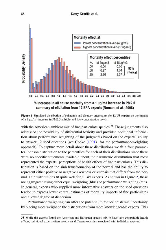
We combine the expert judgments about nonlinearities and causality, weight-ing the judgments equally. The resulting distribution is shown in Figure 1.36 Theblue distribution (probability distribution for mortality effect per 1 µg/m3 reduc-tion in fine particulates) has a higher spike at 0 (indicating the judgments of non-causality) than the red distribution. The blue distribution represents the probabilitydistribution for reductions less than 7 µg/m3 while the red distribution representsthe probability distribution for reductions at higher ambient levels over 16 µg/m3.The experts, on the whole, expect some non-causality/nonlinearity at lower concen-trations, but not large nonlinearities.37
3.4 Performance weighting and additional expert elicitations
The expert elicitation in Cooke et al. (2007) and Tuomisto, Wilson, Evans andTainio (2007) provided six more expert judgments about health effects associated
36 In many cases the experts provided enough information about a parametric distribution, possiblytruncated, that they specifically chose to fit the parameters to that distribution directly. In other cases,the experts chose nonparametric distributions that were more difficult for us to fit. Expert B chose abimodal distribution that would not fit most parametric distributions that assume unimodality. We useda piecewise uniform distribution to fit it, preserving all the characteristics about quantiles. In other caseswhere no specific distribution was chosen we used a four parameter Johnson distribution. We simulated100,000 draws from each expert distribution and then merged the data together to generate the combineddistribution representing the synthesis of the unconditional distributions for all experts.37 Some of the more recent studies such as Krewski et al. (2009) and Lepeule et al. (2012) hint at apotential supralinearity (that is, the concentration–response relationship is steeper at low concentrationsthan at high ones). Such a finding might also be the result of failures to adequately control for timevarying confounding variables like medical advances. Over time, as the concentration of fine particulatesis reduced by less each year, this reduction is related to the same improvement in medicine. This couldmake a sublinear relationship look more linear.
88 Kerry Krutilla et al.
Figure 1 Simulated distribution of epistemic and aleatory uncertainty for 12 US experts on the impactof a 1 µg/m3 increase in PM2.5 at high- and low-concentration levels.
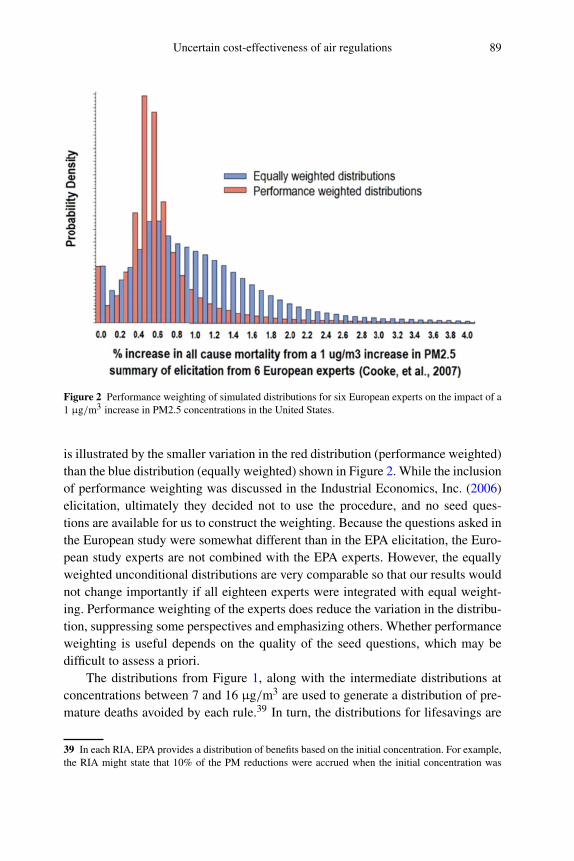
with the American ambient mix of fine particulate species.38 These judgments alsoaddressed the possibility of differential toxicity and provided additional informa-tion about performance weighting of the judgments based on the experts’ abilityto answer 12 seed questions (see Cooke (1991) for the performance-weightingapproach). To capture more detail about these distributions we fit a four parame-ter Johnson distribution to the percentiles for each of their distributions since therewere no specific statements available about the parametric distribution that mostrepresented the experts’ perceptions of health effects of fine particulates. This dis-tribution is based on the sinh transformation of the normal and has the ability torepresent either positive or negative skewness or kurtosis that differs from the nor-mal. Our distributions fit quite well for all six experts. As shown in Figure 2, theseare aggregated using either equal weighting (blue) or performance weighting (red).In general, experts who supplied more informative answers on the seed questionstended to express lower central estimates of mortality impacts of fine particulatesand a lower degree of dispersion.
Performance weighting can offer the potential to reduce epistemic uncertaintyby placing more weight on the distributions from more knowledgeable experts. This
38 While the experts found the American and European species mix to have very comparable healtheffects, individual experts often noted very different toxicities associated with individual species.
Uncertain cost-effectiveness of air regulations 89
Figure 2 Performance weighting of simulated distributions for six European experts on the impact of a1 µg/m3 increase in PM2.5 concentrations in the United States.
is illustrated by the smaller variation in the red distribution (performance weighted)than the blue distribution (equally weighted) shown in Figure 2. While the inclusionof performance weighting was discussed in the Industrial Economics, Inc. (2006)elicitation, ultimately they decided not to use the procedure, and no seed ques-tions are available for us to construct the weighting. Because the questions asked inthe European study were somewhat different than in the EPA elicitation, the Euro-pean study experts are not combined with the EPA experts. However, the equallyweighted unconditional distributions are very comparable so that our results wouldnot change importantly if all eighteen experts were integrated with equal weight-ing. Performance weighting of the experts does reduce the variation in the distribu-tion, suppressing some perspectives and emphasizing others. Whether performanceweighting is useful depends on the quality of the seed questions, which may bedifficult to assess a priori.
The distributions from Figure 1, along with the intermediate distributions atconcentrations between 7 and 16 µg/m3 are used to generate a distribution of pre-mature deaths avoided by each rule.39 In turn, the distributions for lifesavings are
39 In each RIA, EPA provides a distribution of benefits based on the initial concentration. For example,the RIA might state that 10% of the PM reductions were accrued when the initial concentration was
90 Kerry Krutilla et al.
used to construct confidence intervals for the different cost-effectiveness metricsused in the study.
3.5 Cost-effectiveness measures
In this section, we discuss the cost-effectiveness ratios used in the study. Numera-tors are constructed by subtracting some of the benefits other than lifesavings fromcompliance costs, giving a “net cost,” while denominators are represented as livessaved, life years saved, or QALYs gained. The methods used to derive the vari-ous cost-effectiveness measures follow the standard practice for cost-effectivenessanalysis in the health evaluation field (Robinson & Hammitt, 2013), and in theextensions made to the assessment of air quality regulations (Robinson et al., 2005;U.S. EPA, 2006; Hubbell, 2006; Cohen, Hammitt & Levy, 2003).
The categories of health benefits that are typically monetized in EPA RIAsare shown in Table 3, with an example valuation based on central estimates fromthe CSAPR. The pattern displayed is typical for the rules in the study. Mortalitybenefits are significantly larger than morbidity benefits. For the morbidity cate-gory, chronic bronchitis and non-fatal heart attacks are the largest components.40
The RIAs derive estimates of the effects of air regulations and their valuationfrom a variety of sources. Avoided cases of chronic bronchitis and non-fatal heartattacks are derived respectively from health impact functions from Abbey, Hwang,Burchette, Vancuren and Mills (1995) and Peters, Dockery, Muller and Mittleman(2001). A willingness to pay study by Viscusi, Magat and Huber (1991) is the start-ing point for the valuation of chronic bronchitis.41 A cost of illness (COI) valuationwith two components – medical costs and work productivity – is used to value non-fatal myocardial infarctions. A study by Wittels, Hay and Gotto Jr. (1990) providesthe estimates for the medical costs, while Cropper and Krupnick (1990) is used tovalue lost earnings. A variety of mostly COI studies are used to determine valuesfor the other morbidity categories shown in Table 3.
between 10–11 µg/m3. Ideally, we would use a distribution of benefits associated with 11–10 µg/m3
for the first unit of reduction, and 10–9 µg/m3 for the second unit, and so on. However, since we donot know the distribution of reductions, this is not possible. Instead, we use the impact for 10–11 forall reductions that start at this concentration. The ultimate result is that this approach tends to overstatebenefits slightly, particularly at locations where the magnitude of reductions is large.40 EPA stopped monetizing the value of reducing chronic bronchitis starting with the RIA for theNAAQS for PM. But the RIAs for all of the rules in our sample monetize the value of reducing chronicbronchitis.41 See the CSAPR RIA pdf pp. 119–120.

Uncertain cost-effectiveness of air regulations 91
Table 3 Health endpoints and their evaluation for the Cross State Air Pollution Rule.
Morbidity Health end point Mean total value(Billions $2007)
Duration more than 1 year Mortality $100/$2701
Chronic bronchitis $4.2
Non-fatal heart attacks $1.72
Duration less than 1 year Hospital admissions-respiratory $.04
Hospital admissions-cardiovascular $.09
Hospital admissions asthma-related ER $.003
Acute bronchitis $.008
Upper respiratory symptoms $.005
Lower respiratory symptoms $.004
Asthma exacerbations $.02
Work loss $.2
School absence $.01
Minor restricted activity $.7
1Estimates from American Cancer Society Study and Harvard Six Cities Study respectively.23% discount rate.
Energy savings and diminished carbon emissions are sometimes valued in theRIAs, and visibility benefits are monetized for the CSAPR. We use the centralbenefit estimates given in the RIAs for the monetary valuation of these categories,and also for the morbidity benefits.42
From the benefits monetized in the RIAs, two “net cost” numerators are con-structed. The first subtracts all benefits from the rule’s compliance costs other thanthe value of avoided mortality. We denote the result as the “low net cost boundary.”It is possible for this subtraction to yield a negative number, implying that the non-mortality benefits alone are sufficient to cover the compliance costs of the rule. Inthis case, the regulation is denoted as “cost saving,” and no further computation isconducted.
When QALYs are used to represent outcomes, a second net cost numerator iscomputed. Two adjustments are made to the first measure. The productivity part of
42 There has been some recent discussion about the appropriate accounting stance for valuing global cli-mate benefits. Gayer and Viscusi (2014) argue that the accounting perspective should be national, whichis consistent with the general recommendation in OMB Circular A-4. The national accounting stancereduces the Social Cost of Carbon to 7–10% of its total value if U.S. benefit estimates are derived directlyfrom integrated assessment models, and to 23% if it is assumed that the U.S. share of climate benefitsis proportional to the share of the U.S. economy in global GDP. However, for the rules in the study thatestimate climate benefits, the benefits were relatively small. Given that it does not matter very much, wedid not adjust the global warming benefit estimates in the RIAs to the U.S. accounting perspective.
92 Kerry Krutilla et al.
the COI estimate for non-fatal heart attacks is excluded, rather than subtracted, inthe numerator computation. This adjustment reflects the common point of viewin the health evaluation literature that productivity is represented in the QALYmeasure in the denominator.43 The morbidity estimate for chronic bronchitis isalso excluded from the numerator. In theory, the medical cost part of the estimateshould be subtracted from the compliance cost while the other components shouldbe removed on the assumption that productivity and utility gains are representedby the QALY measure in the denominator (Institute of Medicine, 2006). However,there is no empirical basis to make this discrimination. Consequently, chronic bron-chitis is fully excluded. This results in a high net cost boundary. These two net costmeasures bracket the formats discussed in the literature on cost–utility analysis.
Table 4 shows the two net cost numerators. Two of the rules, the CSAPR andNSPS for Petroleum Refineries, are cost savings in all of the permutations. Thevisibility benefit and the value of avoided bronchitis for the CSAPR rule are eachabove $4 billion, while compliance costs are $2.6 billion. As noted before, thenegative net cost for the Petroleum Refinery rule comes from energy savings. TheBoiler MACT rule is also cost saving at 3% for the low-bound numerator. Thisrule significantly reduces chronic bronchitis and myocardial infarctions, and theassociated benefits lower net costs. For the other rules, the benefits are less than thecompliance costs, so they have positive net cost numerators.44
Turning to the outcome side, none of the RIAs in our study provided esti-mates of lives saved by age class. This information is necessary for estimating lifeyears gained. Additionally, for the six rules in our study using the “benefit per ton”approach, there is no information on the fine level geographic detail that wouldshow how pollutant concentrations might be correlated with age class. To deal withthis informational constraint, we assume that age distributions are independent ofconcentrations and use fairly course state level information about mortality inci-dence rates to estimate life year savings. This approach may not lead to signifi-cant biases given the need for spatial aggregation for benefit analysis (see Smith& Gans, 2014). As a point of comparison, our estimates of undiscounted life yearsper life saved are 15.31, 15.49, and 15.31 using age-class mortality incidence datafor the eastern states covered by the CSAPR, the 32 states covered by the NSPSfor Petroleum refineries, and the entire United States. These figures compare withestimates given in the RIA for the NAAQS for PM of 15.0 using the ACS studyand 16.0 using the SCS study. In short, our method gives life year estimates in
43 See Tilling et al. (2012) and U.S. EPA (2006) for a discussion of this issue.44 A number of benefits are not monetized in EPA RIAs, e.g., the health and morbidity benefits associ-ated with the reduction of other pollutants than PM2.5. Adding the monetary valuation of these omittedbenefits would reduce the net cost ratios.

Uncertain
cost-effectivenessofairregulations
93
Table 4 Two net costs (gross compliance cost less benefits) for numerators.
Rule Low Bound ($2013 000’)*
(Used in all ratios)High Bound ($2013 000’)*
(Used only with QALY denominators)
3% 7% 3% 7%
Mercury and air toxic standards (MATS) 7,600,000 7,800,000 9,600,000 9,800,000
Cross state air pollution rule (CSAPR) Cost saving Cost saving Cost saving Cost saving
National emissions standards for hazardousair pollutants (NESHAP) for major boilers(“Boiler MACT”)
Cost saving $18,000 $970,000 $970,000
National emissions standards for hazardousair pollutants (NESHAP) for area sourceboilers
$520,000 $520,000 $520,000 $520,000
NESHAP for commercial and industrialsolid waste incinerators
$250,000 $250,000 $270,000 $270,000
NESHAP for the portland cement manufac-turing industry and performance standardsfor portland cement plants
$550,000 $560,000 $870,000 $870,000
NESHAP for compression ignited recip-rocating internal combustion engines(CIRICE)
$350,000 $350,000 $370,000 $370,000
NESHAP for spark-ignited reciprocatinginternal combustion engines (SIRICE)
$120,000 $120,000 $120,000 $120,000
New source performance standards (NSPS)for petroleum refineries
Cost saving Cost saving Cost saving Cost saving
∗Estimates are rounded to two significant figures. The difference between the 3% and 7% discount rates is sometimes not apparent at two significant figures.

94 Kerry Krutilla et al.
the neighborhood of those that EPA has estimated in an RIA based on air qualitymodeling.45
Following the Institute of Medicine (2006) and U.S. EPA (2006), QALYs werecomputed for the avoided incidences of chronic bronchitis and myocardial infarc-tions. Incidence of these morbidity categories by age group were taken from datacompiled by the U.S. Department of Health and Human Services (2012, 2014)and the National Hospital Discharge Survey (Hall, DeFrances, Williams, Golosin-skiy & Schwartzman, 2010). Following U.S. EPA (2006), individuals with chronicbronchitis were assumed to have normal lifespans.46 For non-fatal heart attacks,assumptions about life spans and the probability of various health conditions afterheart attacks were taken from U.S. EPA (2006, pdf pp. 20–24). With utility weights,this information gives the expected QALYs saved from reducing non-fatal heartattacks.
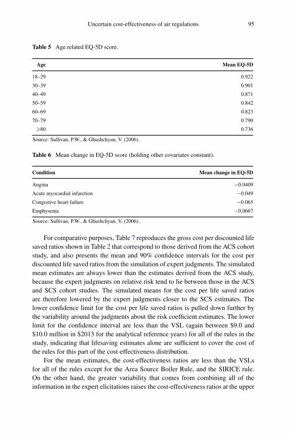
Preference-based EQ-5D scores are used for utility weights, as recommendedby the Institute of Medicine (2006). These scores are taken from a regression studyby Sullivan and Ghushchyan (2006), based on data from the Medical Expendi-ture Panel Survey. Coefficient estimates from this regression give the marginalchanges in EQ-5D scores as a function of various health conditions. The Sulli-van and Ghushchyan study also gives age-based EQ-5D utility weights for baselinehealth status. We adjust baseline health status to reflect age, as recommended bythe Institute of Medicine (2006).
The weights used in our study are shown in Tables 5 and 6. Notice that thedecline in utility associated with the change in health status from aging is largerthan the decline in utility from the health state change associated with any onecategory of morbidity, holding all else constant.
4 Results
Cost-effectiveness ratios are displayed in Tables 7–11. For illustrative purposes,the ratios are shown for the 3% discount rate. With the exception of the BoilerMACT rule, the difference between the 3% and 7% rates does not significantlyaffect results. (Again see Table 4).
45 Data for mortality incidence by age class are from an online data base, CDC Wonder. We averagedthe percentage of the age-specific mortality across 3 years (2004 through 2006). Once the age distribu-tions were determined, discounted life years were computed for each age class based on the age-specificconditional lifespans. These discounted life years were then aggregated.46 This assumption provides an upward biased estimate of the QALYS gained from avoiding chronicbronchitis if individuals with chronic bronchitis do not have normal lifespans.
Uncertain cost-effectiveness of air regulations 95
Table 5 Age related EQ-5D score.
Age Mean EQ-5D
18–29 0.922
30–39 0.901
40–49 0.871
50–59 0.842
60–69 0.823
70–79 0.790
>80 0.736
Source: Sullivan, P.W., & Ghushchyan, V. (2006).
Table 6 Mean change in EQ-5D score (holding other covariates constant).
Condition Mean change in EQ-5D
Angina −0.0409
Acute myocardial infarction −0.049
Congestive heart failure −0.065
Emphysema −0.0667
Source: Sullivan, P.W., & Ghushchyan, V. (2006).
For comparative purposes, Table 7 reproduces the gross cost per discounted lifesaved ratios shown in Table 2 that correspond to those derived from the ACS cohortstudy, and also presents the mean and 90% confidence intervals for the cost perdiscounted life saved ratios from the simulation of expert judgments. The simulatedmean estimates are always lower than the estimates derived from the ACS study,because the expert judgments on relative risk tend to lie between those in the ACSand SCS cohort studies. The simulated means for the cost per life saved ratiosare therefore lowered by the expert judgments closer to the SCS estimates. Thelower confidence limit for the cost per life saved ratios is pulled down further bythe variability around the judgments about the risk coefficient estimates. The lowerlimit for the confidence interval are less than the VSL (again between $9.0 and$10.0 million in $2013 for the analytical reference years) for all of the rules in thestudy, indicating that lifesaving estimates alone are sufficient to cover the cost ofthe rules for this part of the cost-effectiveness distribution.
For the mean estimates, the cost-effectiveness ratios are less than the VSLsfor all of the rules except for the Area Source Boiler Rule, and the SIRICE rule.On the other hand, the greater variability that comes from combining all of theinformation in the expert elicitations raises the cost-effectiveness ratios at the upper
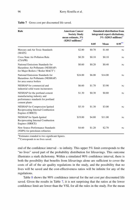
96 Kerry Krutilla et al.
Table 7 Gross cost per discounted life saved.
Rule American CancerSociety Study
mean estimate, 3%($2013 millions)*
Simulated distribution fromintegrated expert elicitations,
3% ($2013 millions)*
0.05 Mean 0.95**
Mercury and Air Toxic Standards(MATS)
$2.80 $0.70 $1.60 ∞
Cross State Air Pollution Rule(CSAPR)
$0.20 $0.10 $0.10 ∞
National Emissions Standards forHazardous Air Pollutants (NESHAP)for Major Boilers (“Boiler MACT”)
$0.60 $0.20 $0.40 ∞
National Emissions Standards forHazardous Air Pollutants (NESHAP)for area source boilers
$24.00 $6.00 $14.00 ∞
NESHAP for commercial andindustrial solid waste incinerators
$6.60 $1.70 $3.90 ∞
NESHAP for the portland cementmanufacturing industry andperformance standards for portlandcement plants
$1.30 $0.30 $0.80 ∞
NESHAP for Compression IgnitedReciprocating Internal CombustionEngines (CIRICE)
$5.10 $1.30 $3.00 ∞
NESHAP for Spark-IgnitedReciprocating Internal CombustionEngines (SIRICE)
$19.00 $4.80 $11.00 ∞
New Source Performance Standards(NSPS) for petroleum refineries
$4.60 $1.20 $2.70 ∞
∗Estimates rounded to two significant figures.∗∗Corresponds to no lives saved.
end of the confidence interval – to infinity. This upper 5% limit corresponds to the“no lives” saved part of the probability distribution for lifesavings. This outcomeillustrates a stark dichotomy. Within a simulated 90% confidence interval, there isboth the possibility that benefits from lifesavings alone are sufficient to cover thecosts of all of the air quality regulations in the study, and the possibility that nolives will be saved and the cost-effectiveness ratios will be infinite for any of theregulations.
Table 8 shows the 90% confidence interval for the net cost per discounted lifesaved. Given the results in Table 7, it is not surprising that the ratios at the lowerconfidence limit are lower than the VSL for all the rules in the study. For the mean

Uncertain cost-effectiveness of air regulations 97
Table 8 Net cost per discounted life saved.
Rule American CancerSociety Study
mean estimate, 3%($2013 000’)*
Simulated distribution from integratedexpert elicitations, 3% ($2013 000’)*
0.05 Mean 0.95**
Mercury and Air ToxicStandards (MATS)
$2,000 $510 $1,200 ∞
Cross State Air PollutionRule (CSAPR)
Cost saving Cost saving Cost saving Cost saving
National EmissionsStandards for HazardousAir Pollutants (NESHAP)for Major Boilers (“BoilerMACT”)
Cost saving Cost saving Cost saving Cost saving
National EmissionsStandards for HazardousAir Pollutants (NESHAP)for area source boilers
$22,000 $5500 $13,200 ∞
NESHAP for commercialand industrial solid wasteincinerators
$5,900 $1,500 $3,500 ∞
NESHAP for the portlandcement manufacturingindustry and performancestandards for portlandcement plants
$630 $160 $370 ∞
NESHAP for CompressionIgnited ReciprocatingInternal CombustionEngines (CIRICE)
$4,500 $1,100 $2,700 ∞
NESHAP for Spark-IgnitedReciprocating InternalCombustion Engines(SIRICE)
$18,000 $4,700 $11,000 ∞
New Source PerformanceStandards (NSPS) forpetroleum refineries
Cost saving Cost saving Cost saving Cost saving
∗Estimates rounded to two significant figures.∗∗Corresponds to no lives saved.
estimates, the ratios are less than the VSL with the exception of the Area SourceBoiler Ruler and the SIRICE rule. These results are again consistent with those inTable 7, and are also consistent with the sign of the net benefits estimated for these
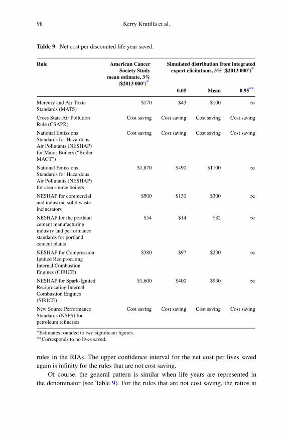
98 Kerry Krutilla et al.
Table 9 Net cost per discounted life year saved.
Rule American CancerSociety Study
mean estimate, 3%($2013 000’)*
Simulated distribution from integratedexpert elicitations, 3% ($2013 000’)*
0.05 Mean 0.95**
Mercury and Air ToxicStandards (MATS)
$170 $43 $100 ∞
Cross State Air PollutionRule (CSAPR)
Cost saving Cost saving Cost saving Cost saving
National EmissionsStandards for HazardousAir Pollutants (NESHAP)for Major Boilers (“BoilerMACT”)
Cost saving Cost saving Cost saving Cost saving
National EmissionsStandards for HazardousAir Pollutants (NESHAP)for area source boilers
$1,870 $490 $1100 ∞
NESHAP for commercialand industrial solid wasteincinerators
$500 $130 $300 ∞
NESHAP for the portlandcement manufacturingindustry and performancestandards for portlandcement plants
$54 $14 $32 ∞
NESHAP for CompressionIgnited ReciprocatingInternal CombustionEngines (CIRICE)
$380 $97 $230 ∞
NESHAP for Spark-IgnitedReciprocating InternalCombustion Engines(SIRICE)
$1,600 $400 $930 ∞
New Source PerformanceStandards (NSPS) forpetroleum refineries
Cost saving Cost saving Cost saving Cost saving
∗Estimates rounded to two significant figures.∗∗Corresponds to no lives saved.
rules in the RIAs. The upper confidence interval for the net cost per lives savedagain is infinity for the rules that are not cost saving.
Of course, the general pattern is similar when life years are represented inthe denominator (see Table 9). For the rules that are not cost saving, the ratios at
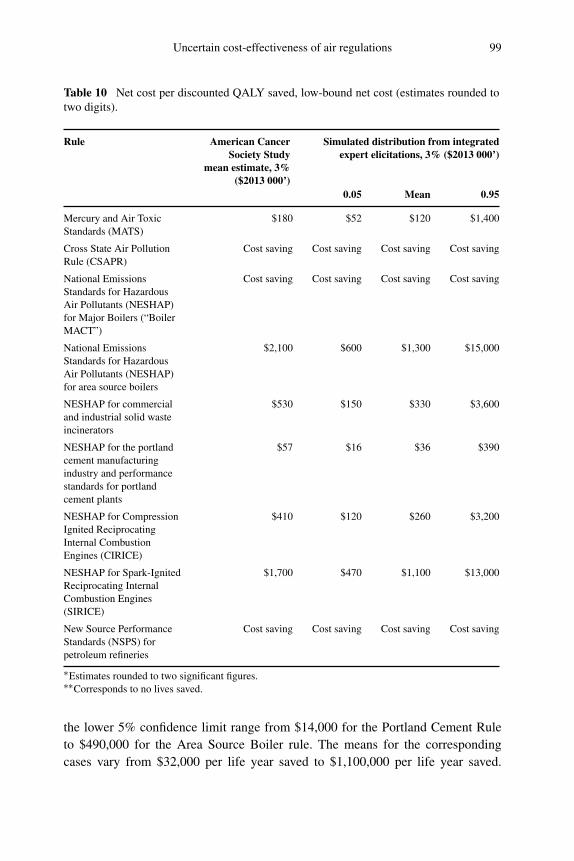
Uncertain cost-effectiveness of air regulations 99
Table 10 Net cost per discounted QALY saved, low-bound net cost (estimates rounded totwo digits).
Rule American CancerSociety Study
mean estimate, 3%($2013 000’)
Simulated distribution from integratedexpert elicitations, 3% ($2013 000’)
0.05 Mean 0.95
Mercury and Air ToxicStandards (MATS)
$180 $52 $120 $1,400
Cross State Air PollutionRule (CSAPR)
Cost saving Cost saving Cost saving Cost saving
National EmissionsStandards for HazardousAir Pollutants (NESHAP)for Major Boilers (“BoilerMACT”)
Cost saving Cost saving Cost saving Cost saving
National EmissionsStandards for HazardousAir Pollutants (NESHAP)for area source boilers
$2,100 $600 $1,300 $15,000
NESHAP for commercialand industrial solid wasteincinerators
$530 $150 $330 $3,600
NESHAP for the portlandcement manufacturingindustry and performancestandards for portlandcement plants
$57 $16 $36 $390
NESHAP for CompressionIgnited ReciprocatingInternal CombustionEngines (CIRICE)
$410 $120 $260 $3,200
NESHAP for Spark-IgnitedReciprocating InternalCombustion Engines(SIRICE)
$1,700 $470 $1,100 $13,000
New Source PerformanceStandards (NSPS) forpetroleum refineries
Cost saving Cost saving Cost saving Cost saving
∗Estimates rounded to two significant figures.∗∗Corresponds to no lives saved.
the lower 5% confidence limit range from $14,000 for the Portland Cement Ruleto $490,000 for the Area Source Boiler rule. The means for the correspondingcases vary from $32,000 per life year saved to $1,100,000 per life year saved.
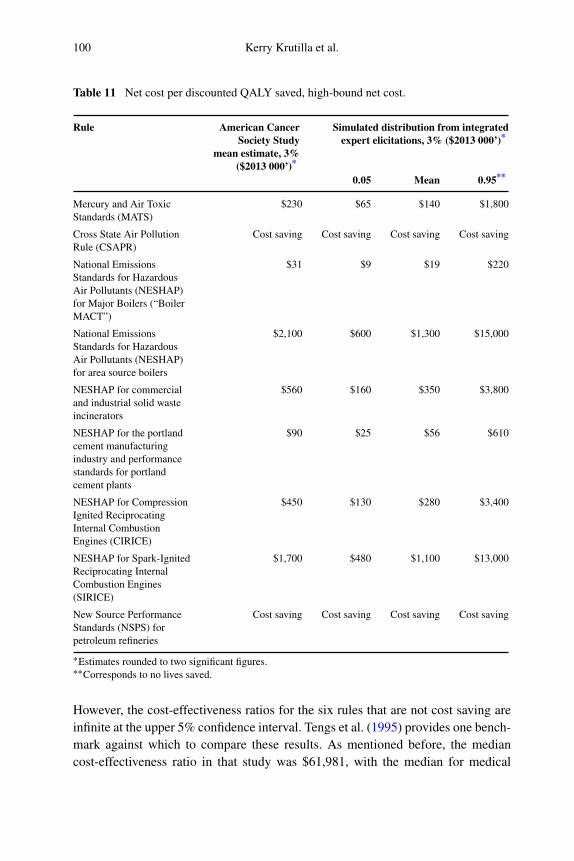
100 Kerry Krutilla et al.
Table 11 Net cost per discounted QALY saved, high-bound net cost.
Rule American CancerSociety Study
mean estimate, 3%($2013 000’)*
Simulated distribution from integratedexpert elicitations, 3% ($2013 000’)*
0.05 Mean 0.95**
Mercury and Air ToxicStandards (MATS)
$230 $65 $140 $1,800
Cross State Air PollutionRule (CSAPR)
Cost saving Cost saving Cost saving Cost saving
National EmissionsStandards for HazardousAir Pollutants (NESHAP)for Major Boilers (“BoilerMACT”)
$31 $9 $19 $220
National EmissionsStandards for HazardousAir Pollutants (NESHAP)for area source boilers
$2,100 $600 $1,300 $15,000
NESHAP for commercialand industrial solid wasteincinerators
$560 $160 $350 $3,800
NESHAP for the portlandcement manufacturingindustry and performancestandards for portlandcement plants
$90 $25 $56 $610
NESHAP for CompressionIgnited ReciprocatingInternal CombustionEngines (CIRICE)
$450 $130 $280 $3,400
NESHAP for Spark-IgnitedReciprocating InternalCombustion Engines(SIRICE)
$1,700 $480 $1,100 $13,000
New Source PerformanceStandards (NSPS) forpetroleum refineries
Cost saving Cost saving Cost saving Cost saving
∗Estimates rounded to two significant figures.∗∗Corresponds to no lives saved.
However, the cost-effectiveness ratios for the six rules that are not cost saving areinfinite at the upper 5% confidence interval. Tengs et al. (1995) provides one bench-mark against which to compare these results. As mentioned before, the mediancost-effectiveness ratio in that study was $61,981, with the median for medical
Uncertain cost-effectiveness of air regulations 101
interventions at $28,039 and those for toxin control of $4.1 million. It seemsunlikely that the median estimates in our study would be less than the $61,981 fig-ure for any of the rules but for portland cement manufacturing (which has a meanestimate of $32,000). Thus, if lower than the median in Tengs et al. (1995) is takenas a metric for relative cost-effectiveness, some regulations in our study havingpositive net benefits (having net cost per life saved less than the VSL) will not meetthis standard – suggesting that different ratio formats can have different normativeimplications. Regardless, uncertainty about the lifesaving effects of the regulationsreconciles the normative standards at the upper confidence limit in which no livesare saved and the regulations with positive net costs are not cost-effective by anymeasure.
Table 10 indicates the net cost per QALY saved by each of the rules using thelow-bound numerator (Again see Table 4). At the lower 5% confidence limit, thenet cost per QALY of all of the rules is less than $200,000 except for the AreaSource Boiler rule, and the SIRICE rule. At the mean, only the MATS and thePortland Cement Rule have net cost per QALY less than $200,000. At the upper5% limit, the net cost per QALY ratios are finite, reflecting the utility gains fromreducing cases of chronic bronchitis and non-fatal heart attacks even without anylifesavings. But the net cost per QALY ratios at this point are relatively high. At theupper 5% limit, all of the rules with positive net cost ratios have net cost per QALYvalues above $200,000.
Table 11 shows the boundary case for the high net cost numerator. In this case,the Boiler MACT rule is not cost saving, but it is the lowest cost rule of any of therules that have positive net costs. The 90% confidence for the net cost per QALY forthis rule runs from $9,000 to $220,000. For the group of other rules having positivenet costs, the ratios are marginally higher than those reported for the high net costbound in Table 10, with the overall pattern being consistent.
In the health evaluation literature, $50,000–$100,000 per QALY gained hasbeen a traditional benchmark for gauging cost-effectiveness (Grosse, 2008). Morerecently, thresholds from $100,000 to $200,000 have been suggested (Neumann,Cohen & Weinstein, 2014). Although widely used, cost-effectiveness benchmarkshave been criticized as arbitrary (Neumann et al., 2014), and for not reflecting rel-evant WTP measures very well (Grosse, 2008). Even with these criticisms, thesebenchmarks provide another reference point for how the cost-effectiveness of airregulations might be regarded in the health evaluation literature. The ratios thatare cost savings are cost-effective by definition. For those regulations with positivenet costs, the air quality interventions would not be regarded as cost-effective forratios at the upper 5% limit. With the exception of the Boiler MACT for the lownet cost boundary, none of the net cost per QALY figures is close to $200,000 per

102 Kerry Krutilla et al.
year at the upper 5% limit. This suggests that, without mortality risk reductions,the values now monetized in RIAs are not alone likely to make air regulations lookcost-effective by the conventional standards of cost–utility analysis.
On the other hand, mortality risk reductions occurring at the mean and lower5% confidence limits significantly lower the net cost per QALY figures. As notedabove, all rules have net cost per QALY lower than $200,000 at the lower 5% confi-dence limit with the exception of the Area Source Boiler rule and the SIRICE rule.For the mean estimates, the picture is more mixed. The mixed picture at the meanagain shows that the normative conclusions drawn from different cost-effectivenessmetrics – cost–utility analysis in this case – may not dovetail with benefit-cost anal-ysis. Specifically, while the mean estimates for net cost per QALY in Tables 10and 11 do not necessarily fall under the $200,000 benchmark, the means for theratios in Table 8 are less than the VSL – again with the exception of the SIRICEand Area Source Boiler rules – indicating that they pass the benefit-cost test.
5 Discussion and conclusion
We have studied recent EPA regulations targeting stationary source air emissions,and have simulated a 90% confidence interval for the premature deaths avoided byeach regulation. These simulations are based on the combined judgments of expertsconcerning the relationship between airborne particulate exposures and mortalityrisks. Adding estimates for compliance cost and morbidity benefits gives 90% con-fidence intervals for cost-effectiveness ratios.
Two of the rules in the sample, the CSAPR and the NSPS for PetroleumRefineries, are “cost saving” in all permutations. That is, the non-mortality ben-efits that these rules provide are sufficient to pay off the compliance costs of therules. The Boiler MACT is also cost saving for the 3% discount rate and lowerbound estimate for its net cost numerator. Of the rules having positive net costs,the net cost-effectiveness ratios differ significantly between the lower and upperconfidence limits. Most of the rules are cost-effective by most metrics at the lower5% confidence bound, while most of the rules are not cost-effective measured byany metric at the upper 5% confidence limit. In particular, all rules with positivenet costs have infinite cost-effectiveness ratios at the upper 5% limit when thedenominators are lives or life years saved. At the mean, the picture is more varied.
Structural aspects of air regulation explain the width of the 90% confidenceintervals for cost-effectiveness ratios. Air pollution creates exposure risks for vir-tually everyone. Small changes in the estimates of relative risk will therefore givelarge changes in estimated mortality risk reductions. The sensitivity of predictions
Uncertain cost-effectiveness of air regulations 103
about total lives saved to minor differences in relative risk estimates suggests theimportance of resolving informational uncertainty about the effects of fine particleexposures on mortality risks.
Our work has focused on particular aspects of epistemic and aleatory uncer-tainty in concentration–response models, but not on others such as the toxicity ofdifferent fine particulate species. To include these uncertainties would have widenedthe confidence intervals further. At the same time, it should be recognized that theexisting expert elicitation studies are more than eight years old and could over-state, as well as understate, uncertainties about causality, magnitudes of impacts,and nonlinearities. As a result, updated elicitations should be conducted reflectinginformation from recent research, including extensions of the ACS and SCS cohortstudies as well as the integrated science assessment sponsored by the EPA (U.S.EPA, 2009). Experience in the use of expert elicitations has increased, allowing forbetter assessments of uncertainty to more refined questions. An updated elicitationstudy could complement EPA’s ongoing efforts to integrate scientific knowledgeabout the consequences of fine particulate mortality.
We believe our results also contain insights relevant for the larger cost-effectiveness literature. The confidence intervals for cost-effectiveness ratios aroundthe rules in our study are substantially wider than the differences between themeans. However, uncertainties for air regulations are highly correlated, reflect-ing lives saved estimates generated from the same relative risk coefficients. In themore common context of cost-effectiveness analysis, effects across interventionsare not likely to be so strongly correlated. In that case, the results of our study serveas a reminder that confidence intervals are important for cost-effectiveness com-parisons. Standard “league tables” that compare cost-effectiveness ratios usuallycontain point estimates. That begs the question of how much uncertainty there isin the estimates given in these tables, and suggests that interpretations about cost-effectiveness based on comparisons of point estimates be made cautiously. Thepresentation of confidence intervals for cost-effectiveness ratios would also allowan expanded analysis that compares trade-offs in means and variances for differentinterventions.
Acknowledgments and Disclaimer: The authors want to thank the ElectricPower Research Institute for financial support, and to acknowledge the thought-ful oversight of their technical advisory board – Susan Dudley, John Evans, ArtFraas, James K. Hammitt, and Charles Poole. They also appreciate exchanges withEPA’s air quality group – Susan Anenberg, Neal Fann, and Bryan Hubbell – andespecially Amy Lamson, who offered informative responses to numerous queriesand a technical review of the article. Ron Wyzga, Lisa Robinson, Anne Smith,
104 Kerry Krutilla et al.
Elisabeth Gilmore, Kevin Boyle, James Barnes, and Dan Cole offered knowl-edgeable perspectives on various aspects of the work, while Ed Chicanowicz andMark Menefee provided useful information about compliance costs. Yu Zhang,Gabriel Pina, Michelle Hoover, and Tyler Kerr provided capable research assis-tance. Finally, Glenn Blomquist and an anonymous reviewer provided perceptiveand detailed comments on an initial submission of the article, and Mary Kokoskigave the article a necessary editing. While indebted to all of these individuals,the authors are entirely responsible for the execution of the study, its results andconclusions, and the final written article.
Appendix A. Federal register publication of therules in the study
A.1 Utility rules
U.S. EPA, “National Emission Standards for Hazardous Air Pollutants From Coal-and Oil-Fired Electric Utility Steam Generating Units and Standards of Perfor-mance for Fossil-Fuel-Fired Electric Utility, Industrial-Commercial- Institutional,andSmall Industrial-Commercial-InstitutionalSteamGeneratingUnits;FinalRule,”77 Federal Register 9304, February 16, 2012. http://www.gpo.gov/fdsys/pkg/FR-2012-02-16/pdf/2012-806.pdf
U.S. EPA, “Revisions to Federal Implementation Plans To Reduce InterstateTransport of Fine Particulate Matter and Ozone; Final Rule,” 77 Federal Register34830, June 12, 2012. http://www.gpo.gov/fdsys/pkg/FR-2012-06-12/pdf/2012-14251.pdf
A.2 Boilers and incinerators
U.S. EPA, “National Emission Standards for Hazardous Air Pollutants for MajorSources: Industrial, Commercial, and Institutional Boilers and Process Heaters;Final Rule,” 78 Federal Register 7138, January 31, 2013. http://www.gpo.gov/fdsys/pkg/FR-2013-01-31/pdf/2012-31646.pdf
U.S. EPA, “National Emission Standards for Hazardous Air Pollutants for AreaSources: Industrial, Commercial, and Institutional Boilers; Final Rule” 78 FederalRegister 7488, February 1, 2013. http://www.gpo.gov/fdsys/pkg/FR-2013-02-01/pdf/2012-31645.pdf
Uncertain cost-effectiveness of air regulations 105
U.S. EPA, “Commercial and Industrial Solid Waste Incineration Units: Recon-sideration and Final Amendments; Non-Hazardous Secondary Materials That AreSolid Waste; Final Rule,” 78 Federal Register 9112, February 7, 2013. http://www.gpo.gov/fdsys/pkg/FR-2013-02-07/pdf/2012-31632.pdf
A.3 Portland cement
U.S. EPA, “National Emission Standards for Hazardous Air Pollutants for thePortland Cement Manufacturing Industry and Standards of Performance for Port-land Cement Plants; Final Rule,” 78 Federal Register 10006, February 12, 2013.http://www.gpo.gov/fdsys/pkg/FR-2013-02-12/pdf/2012-31633.pdf
A.4 RICE rules
U.S. EPA, “National Emission Standards for Hazardous Air Pollutants for Recipro-cating Internal Combustion Engines; New Source Performance Standards for Sta-tionary Internal Combustion Engines; Final Rule,” 78 Federal Register 6674, Jan-uary 30, 2013. http://www.gpo.gov/fdsys/pkg/FR-2013-01-30/pdf/2013-01288.pdf
A.5 Petroleum refineries
U.S. EPA, “Standards of Performance for Petroleum Refineries for Which Con-struction, Reconstruction, or Modification Commenced After May 14, 2007; FinalRule,” 77 Federal Register 56422, September 12, 2012. http://www.gpo.gov/fdsys/pkg/FR-2012-09-12/pdf/2012-20866.pdf
Appendix B. Regulatory impact analyses
B.1 Utility rules
U.S. EPA, “Regulatory Impact Analysis for the Final Mercury and Air ToxicsStandards,” December 2011. http://www.epa.gov/ttnecas1/regdata/RIAs/matsriafinal.pdf
U.S. EPA, “Regulatory Impact Analysis for the Federal Implementation Plansto Reduce Interstate Transport of Fine Particulate Matter and Ozone in 27 States;

106 Kerry Krutilla et al.
Correction of SIP Approvals for 22 States,” June 2011. http://www.epa.gov/airtransport/pdfs/FinalRIA.pdf
B.2 Boilers and incinerators
U.S. EPA, “Regulatory Impact Results for Reconsideration Final Rule for NationalEmission Standards for Hazardous Air Pollutants for Industrial, Commercial, andInstitutional Boilers and Process Heaters at Major Sources,” December 2012. http://epa.gov/airquality/combustion/docs/boilerreconfinalria121220.pdf
U.S. EPA, “Regulatory Impact Results for the Reconsideration Final Rule forStandards of Performance for New Stationary Sources and Emission Guidelinesfor Existing Sources: Commercial and Industrial Solid Waste Incineration Units,”December 2012. http://epa.gov/airquality/combustion/docs/boilerreconfinalria121220.pdf
U.S. EPA, “Regulatory Impact Analysis: National Emission Standards forHazardous Air Pollutants for Industrial, Commercial, and Institutional Boilers andProcess Heaters,” February 2011. http://epa.gov/airquality/combustion/docs/ciswireconfinalria.pdf
B.3 Portland cement
U.S. EPA, “Regulatory Impact Analysis: Amendments to the National EmissionStandards for Hazardous Air Pollutants and New Source Performance Standards(NSPS) for the Portland Cement Manufacturing Industry,” August 2010. http://www.epa.gov/ttnecas1/regdata/RIAs/portlandcementfinalria.pdf
B.4 RICE rules
U.S. EPA, “Regulatory Impact Analysis for Reconsideration of Existing StationarySpark Ignition Rice NESHAP,” January 2013. http://www.epa.gov/ttnecas1/regdata/RIAs/NESHAP RICE Spark Ignition RIA finalreconsideration2013 EPA.pdf
U.S. EPA, “Regulatory Impact Analysis for the Reconsideration of the ExistingStationary Compression Ignition Engines NESHAP,” January 2013. http://www.epa.gov/ttnecas1/regdata/RIAs/RICE NESHAPreconsideration Compression Ignition Engines RIA final2013 EPA.pdf
Uncertain cost-effectiveness of air regulations 107
B.5 Petroleum refineries
U.S. EPA, “Regulatory Impact Analysis Petroleum Refineries New Source Perfor-mance Standards,” June 2012. http://www.epa.gov/ttnecas1/regdata/RIAs/refineries nsps ja final ria.pdf
References
Abbey, D. E., Hwang, B. L., Burchette, R. J., Vancuren, T. & Mills, P. K. (1995). EstimatedLong-Term Ambient Concentrations of PM10 and Development of Respiratory Symp-toms in a Nonsmoking Population. Archives of Environmental Health: An InternationalJournal, 50(2), 139–152.
Burtraw, D., Palmer, K., Paul, A. & Woerman, M. (2012). Secular Trends, EnvironmentalRegulations, and Electricity Markets. The Electricity Journal, 25(6), 35–47.
Chicanowicz, J. (2011). Factors Affecting the Timeline for Retrofit of Environmental Con-trol Technologies to Coal-fired Power Stations: Testimony before the Subcommitteeon Energy and Environment (Committee on Science, Space and Technology), UnitedStates House of Representatives, 113th Cong.
Cohen, J. T., Hammitt, J. K. & Levy, J. I. (2003). Fuels for Urban Transit Buses: A Cost-Effectiveness Analysis. Environmental Science & Technology, 37(8), 1477–1484.
Cooke, R. M. (1991). Experts in Uncertainty: Opinion and Subjective Probability in Science.New York: Oxford University Press.
Cooke, R., Wilson, A., Tuomisto, J., Morales, O., Tainio, M. & Evans, J. (2007). A Proba-bilistic Characterization of the Relationship between Fine Particulate Matter and Mor-tality: Elicitation of European Experts. Environmental Science & Technology, 41(18),6598–6605.
Cox, L. (2012). Miscommunicating Risk, Uncertainty, and Causation: Fine Particulate AirPollution and Mortality Risk as an Example. Risk Analysis, 32(5), 765–767.
Cropper, M. L. & Krupnick, A. J. (1990). The Social Costs of Chronic Heart and LungDisease. Resources for the Future. Washington, DC. Discussion Paper QE-89-16-REV.
Dockery, D. W., Pope, C. A., Xu, X., Spengler, J. D., Ware, J. H., Fay, M. E., Ferris, B. G. &Speizer, F. E. (1993). An Association Between Air Pollution and Mortality in Six USCities. New England Journal of Medicine, 329(24), 1753–1759.
Drummond, M. F., O’Brien, B., Stoddart, G. L. & Torrance, G. W. (2005). Methods for Eco-nomic Evaluation of Health Care Programmes. (3rd ed.). New York: Oxford MedicalPublications, Oxford University Press.
Fann, N., Gilmore, E. & Walker, K. (2013). Characterizing the Long-term PM2.5 Concentra-tion Response Function: Comparing Strengths and Weaknesses of Research SynthesisApproaches. Working Paper prepared for: Methods for Research Synthesis; A Cross-Disciplinary Workshop, Harvard Center for Risk Analysis.
Fann, N., Lamson, A. D., Anenberg, S. C. & Hubbell, B. J. (2013). Letter in Response toFraas & Lutter Article: Uncertain Benefits Estimates for Reductions in Fine ParticleConcentrations. Risk Analysis, 33(5), 755–756.
Fann, N., Lamson, A. D., Anenberg, S. C., Wesson, K., Risley, D. & Hubbell, B. J. (2012a).Estimating the National Public Health Burden Associated with Exposure to AmbientPM2.5 and Ozone. Risk Analysis, 32(1), 81–95.

108 Kerry Krutilla et al.
Fann, N., Lamson, A. D., Anenberg, S. C., Wesson, K., Risley, D. & Hubbell, B. J. (2012b).Response to Cox Letter: “Miscommunicating Risk, Uncertainty, and Causation: FineParticulate Air Pollution and Mortality Risk as an Example”. Risk Analysis, 32(5), 768.
Fann, N., Lamson, A., Luben, T. & Hubbell, B. (2015). Response To: “Enhancing theCharacterization of Epistemic Uncertainties in PM2.5 Risk Analyses”. Risk Analysis.Advance online publication. doi:10.1111/risa.12301.
Fraas, A. & Lutter, R. (2011). Do Some NOx Emissions Have Negative EnvironmentalDamages? Evidence and Implications for Policy. Environmental Science & Technology,45(18), 7613–7614.
Fraas, A. & Lutter, R. (2012). Efficient Pollution Regulation: Getting the Prices Right: Com-ment. American Economic Review, 102(1), 602–607.
Fraas, A. & Lutter, R. (2013a). Uncertain Benefits Estimates for Reductions in Fine ParticleConcentrations. Risk Analysis, 33(3), 434–449.
Fraas, A. & Lutter, R. (2013b). Reply to Letter by Fann, Lamson, Anenberg, and Hubbell,Regarding Fraas & Lutter Article: Uncertain Benefits Estimates for Reductions in FineParticle Concentrations. Risk Analysis, 33(5), 757–759.
Gayer, T. & Viscusi, W. K. (2014). Determining the Proper Scope of Climate Change Ben-efits. Vanderbilt Law and Economics Research Paper, (14–20). Retrieved from Brook-ings Institute website: http://www.brookings.edu/research/papers/2014/06/04-determining-proper-scope-climate-change-benefits-gayer.
Gillingham, K. & Palmer, K. (2014). Bridging the Energy Efficiency Gap: Policy Insightsfrom Economic Theory and Empirical Evidence. Review of Environmental Economicsand Policy, 8(1), 18–38.
Graham, J. D. (2008). Saving Lives Through Administrative Law and Economics. Universityof Pennsylvania Law Review, 157(2), 395–540.
Grosse, S. D. (2008). Assessing Cost-Effectiveness in Healthcare: History of the $50,000 perQALY Threshold. Expert Review of Pharmacoeconomics & Outcomes Research, 8(2),165–178.
Hall, M., DeFrances, C., Williams, S., Golosinskiy, A. & Schwartzman, A. (2010). NationalHospital Discharge Survey: 2007 Summary, in National Health Statistics Reports. Octo-ber 29, 2010.
Hammitt, J. K. (2013). Admissible Utility Functions for Health, Longevity, and Wealth:Integrating Monetary and Life-Year Measures. Journal of Risk and Uncertainty, 47(3),311–325.
Haninger, K. & Hammitt, J. K. (2011). Diminishing Willingness to Pay Per Quality-AdjustedLife Year: Valuing Acute Foodborne Illness. Risk Analysis, 31(9), 1363–1380.
Harrington, W., Morgenstern, R. D. & Nelson, P. (2000). On the Accuracy of RegulatoryCost Estimates. Journal of Policy Analysis and Management, 19(2), 297–322.
Hazilla, M. & Kopp, R. J. (1990). Social Cost of Environmental Quality Regulations: AGeneral Equilibrium Analysis. Journal of Political Economy, 853–873.
Heinzerling, L. & Ackerman, F. (2002). The Humbugs of the Anti-Regulatory Movement.Cornell Law Review, 87, 648–670.
Hubbell, B. J. (2006). Implementing QALYs in the Analysis of Air Pollution Regulations.Environmental & Resource Economics, 34(3), 365–384.
Industrial Economics, Inc. (2006). Expanded Expert Judgment Assessment of theConcentration-Response Relationship Between PM 2.5 Exposure and Mortality. Pre-pared for the Office of Air Quality Planning and Standards, U.S. Environmental Protec-tion Agency.
Uncertain cost-effectiveness of air regulations 109
Institute of Medicine (2006). Valuing Health for Regulatory Cost-Effectiveness Analysis.Washington, DC: Institute of Medicine of the National Academies.
Kopits, E. (2014). A Retrospective Assessment of the Costs of EPA’s 1998 Locomotive Emis-sion Standards. Journal of Benefit-Cost Analysis, 5(2), 285–314.
Kopits, E., McGartland, A., Morgan, C., Pasurka, C., Shadbegian, R., Simon, N. B. &Wolverton, A. (2014). Retrospective Cost Analyses of EPA Regulations: A Case StudyApproach. Journal of Benefit-Cost Analysis, 5(2), 173–193.
Krewski, D., Jerrett, M., Burnett, R. T., Ma, R., Hughes, E. & Shi, Y. et al. (2009). ExtendedFollow-Up and Spatial Analysis of the American Cancer Society Study Linking Particu-late Air Pollution and Mortality. Health Effects Institute (HEI) Research Report, (140).
Krupnick, A., Morgenstern, R., Batz, M., Nelson, P., Burtraw, D., Shih, J. S. & McWilliams,M. (2006). Not a Sure Thing: Making Regulatory Choices Under Uncertainty. Wash-ington, DC: Resources for the Future.
Krutilla, K. & Alexeev, A. (2012). The Normative Implications of Political Decision-Makingfor Benefit-Cost Analysis. Journal of Benefit-Cost Analysis, 3(2), Article 2.
Krutilla, K. & Alexeev, A. (2014). The Political Transaction Costs and Uncertainties ofEstablishing Environmental Rights. Ecological Economics, 107, 299–309.
Krutilla, K. & Krause, R. (2011). Transaction Costs and Environmental Policy: An Assess-ment Framework and Literature Review. International Review of Environmental andResource Economics, 4(3–4), 261–354.
Laden, F., Schwartz, J., Speizer, F. E. & Dockery, D. W. (2006). Reduction in Fine Partic-ulate Air Pollution and Mortality. American Journal of Respiratory and Critical CareMedicine, 173(6), 667–672.
Lepeule, J., Laden, F., Dockery, D. & Schwartz, J. (2012). Chronic Exposure to Fine Particlesand Mortality: An Extended Follow-Up of the Harvard Six Cities Study from 1974 to2009. Environmental Health Perspectives, 120(7), 965–970.
Lutter, R., Morrall, J. & Viscusi, W. K. (1999). The Cost-Per-Life-Saved Cutoff for Safety-Enhancing Regulations. Economic Inquiry, 37(4), 599–608.
Martin, R., Muuls, M, de Preux, L. B. & Wagner, U. J. (2010). Anatomy of a Paradox:Management Practices, Organizational Structure and Energy Efficiency. Center for Eco-nomic Performance, Working Paper 1039.
McCarthy, J. (2012). EPA’s Boiler MACT: Controlling Emissions of Hazardous Pollutants.Congressional Research Service Report, (R41459).
McCarthy, J. & Copeland, C. (2011). EPA’s Regulation of Coal-fired Power: Is a “TrainWreck” Coming? Congressional Research Service Report, (R41914).
McGarity, T. O. & Ruttenberg, R. (2001). Counting the Cost of Health, Safety, and Environ-mental Regulation. Tex. L. Rev., 80, 1997.
Morgan, C., Pasurka, C. & Shadbegian, R. (2014). Ex Ante and Ex Post Cost Estimates ofthe Cluster Rule and MACT II Rule. Journal of Benefit-Cost Analysis, 5(2), 195–224.
Morrall, J. F., III (2003). Saving Lives: A Review of the Record. Journal of Risk and Uncer-tainty, 27(3), 221–237.
National Research Council (2002). Estimating the Public Health Benefits of Proposed AirPollution Regulations. Washington, DC: National Academies Press.
Neumann, P. J., Cohen, J. T. & Weinstein, M. C. (2014). Updating Cost-Effectiveness –the Curious Resilience of the $50,000-Per-QALY Threshold. New England Journal ofMedicine, 371(9), 796–797.
Office of Management and Budget (2003). Circular A-4: Regulatory Analysis. Washington,DC: Office of Management and Budget.

110 Kerry Krutilla et al.
Office of Management and Budget (2012). Draft Report to Congress on the Benefits andCosts of Federal Regulations and Agency Compliance with the Unfunded MandatesReform Act. Washington, DC: Office of Management and Budget. Retrieved from http://www.whitehouse.gov/sites/default/files/omb/inforeg/2012 cb/2012 cost benefit report.pdf.
Office of Management and Budget (2014). Draft Report to Congress on the Benefits andCosts of Federal Regulations and Agency Compliance with the Unfunded MandatesReform Act. Washington, DC: Office of Management and Budget. Retrieved from http://www.whitehouse.gov/sites/default/files/omb/inforeg/2013 cb/draft 2013 cost benefit report.pdf.
Peters, A., Dockery, D. W., Muller, J. E. & Mittleman, M. A. (2001). Increased Partic-ulate Air Pollution and the Triggering of Myocardial Infarction. Circulation, 103,2810–2815.
Pope, C. A., III, Thun, M. J., Namboodiri, M. M., Dockery, D. W., Evans, J. S., Speizer,F. E. & Heath, C. W., Jr. (1995). Particulate Air Pollution as A Predictor of Mortality inA Prospective Study of US Adults. American Journal of Respiratory and Critical CareMedicine, 151(3 pt 1), 669–674.
Pope, C. A., III, Burnett, R. T., Thun, M. J., Calle, E. E., Krewski, D., Ito, K. & Thurston,G. D. (2002). Lung Cancer, Cardiopulmonary Mortality, and Long-Term Exposure toFine Particulate Air Pollution. Journal of the American Medical Association, 287(9),1132–1141.
Revesz, R. & Livermore, M. (2008). Retaking Rationality: How Cost Benefit Analysis CanBetter Protect the Environment and Our Health. New York: Oxford University Press.
Robinson, L. A. & Hammitt, J. (2013). Skills of the Trade: Valuing Health Risk Reductionsin Benefit-Cost Analysis. Journal of Benefit-Cost Analysis, 4(1), 107–130.
Robinson, L. A., Black, R., Cropper, M., Burnett, R., Hammitt, J., Krupnick, A. & Williams,S. (2005). Alternative Approaches for Estimating Health Related Quality of LifeImpacts: Nonroad Engine Air Emissions Regulation Case Study. In Health, and SafetyRegulation. Institute of Medicine.
Roman, H. A., Walker, K. D., Walsh, T. L., Conner, L., Richmond, H. M., Hubbell, B. J. &Kinney, P. L. (2008). Expert Judgment Assessment of the Mortality Impact of Changesin Ambient Fine Particulate Matter in the US. Environmental Science & Technology,42(7), 2268–2274.
Ryan, S. P. (2012). The Costs of Environmental Regulation in a Concentrated Industry.Econometrica, 80(3), 1019–1061.
Smith, A. E. & Gans, W. (2014). Enhancing the characterization of epistemic uncertaintiesin PM2.5 risk analyses. Risk Analysis. Advance online publication.doi:10.1111/risa.12236.
Sullivan, P. W. & Ghushchyan, V. (2006). Preference-Based EQ-5D Index Scores for ChronicConditions in the United States. Medical Decision Making, 26(4), 410–420.
Tengs, T. O., Adams, M. E., Pliskin, J. S., Safran, D. G., Siegel, J. E., Weinstein, M. C. &Graham, J. D. (1995). Five-Hundred Life-Saving Interventions and their Cost-Effectiveness. Risk Analysis, 15(3), 369–390.
Tengs, T. O. & Graham, J. D. (1996). The Opportunity Costs of Haphazard Social Invest-ments in Life-Saving. In Risks, Costs, and Lives Saved: Getting Better Results fromRegulation (Vol. 167, p. 172). Oxford University Press.
Thorat, T., Cangelosi, M. & Neumann, P. J. (2012). Skills of the Trade: The Tufts Cost-Effectiveness Analysis Registry. Journal of Benefit-Cost Analysis, 3(01), 1–9.

Uncertain cost-effectiveness of air regulations 111
Tilling, M. C., Kro, M., Tsuchiya, A., Brazier, J., van Exel, J. & Brouwer, W. (2012). DoesThe EQ-5D Reflect Lost Earnings? Pharmaco Economics, 30(1), 47–61.
Tuomisto, J. T., Wilson, A., Evans, J. S. & Tainio, M. (2007). Uncertainty in MortalityResponse to Airborne Fine Particulate Matter: Combining European Air PollutionExperts. Reliability Engineering & System Safety, 93(5), 732–744.
U.S. Department of Health and Human Services Summary health statistics for U.S. adults:National Health Interview Survey, (2012), National Center for Health Statistics. Vitaland Health Statistics 10 (260). February 2014.
U.S. EPA (2002). EPA Air Pollution Control Cost Manual (6th ed.). EPA/452/B-02-001.U.S. EPA (2006). U.S. Environmental Protection Agency. Appendix G: Health-Based Cost-
Effectiveness of Reductions in Ambient PM2.5 Associated with Illustrative PM NAAQSAttainment Strategies. 2006 National Ambient Air Quality Standards for Particle Pollu-tion. Washington, DC: U.S. EPA. Retrieved from http://www.epa.gov/ttnecas1/regdata/RIAs/Appendix%20G--Health%20Based%20Cost%20Effectiveness%20Analysis.pdf.
U.S. EPA (2009). Integrated Science Assessment for Particulate Matter (Final Report). U.S.Environmental Protection Agency, Washington, DC, EPA/600/R-08/139F.
U.S. EPA (2012). Regulatory Impact Analysis for the Final Revisions to the National Ambi-ent Air Quality Standards for Particulate Matter, December 2012. Retrieved fromhttp://www.epa.gov/ttnecas1/regdata/RIAs/finalria.pdf.
U.S. EPA (2014). Guidelines for Preparing Economic Analyses. Washington, DC: U.S. EPAOffice of Policy. (Original work published 2010.) Retrieved from http://yosemite.epa.gov/ee/epa/eerm.nsf/vwAN/EE-0568-50.pdf/$file/EE-0568-50.pdf.
Viscusi, W. K. (2005 − 2006). Monetizing the Benefits of Risk and Environmental Regula-tion. Fordham Urban Law Journal, 33(4), 101–143.
Viscusi, W. K., Magat, W. A. & Huber, J. (1991). Pricing Environmental Health Risks:Survey Assessments of Risk-Risk and Risk-Dollar Trade-Offs for Chronic Bronchitis.Journal of Environmental Economics and Management, 21(1), 32–51.
Wittels, E. H., Hay, J. W. & Gotto, A. M., Jr. (1990). Medical Costs of Coronary ArteryDisease in the United States. American Journal of Cardiology, 65(7), 432–440.