journal of applied science and agriculture 2014/1-15.pdf · journal of applied science and...

Journal of Applied Science and Agriculture, 9(14) September 2014, Pages: 1-15

AENSI Journals

Journal of Applied Science and Agriculture ISSN 1816-9112

Journal home page: www.aensiweb.com/JASA

Corresponding Author: Mohammad Sohrabi, Department of Computer Engineering, South Tehran Branch, Islamic Azad

University, Tehran, Iran

Distributed Fault Detection Method and Diagnosis of Fault Type in Clustered Wireless

Sensor Networks 1Mohammad Sohrabi,

1Mitra Daneshmand,

1Mahsa Daneshmand,

1Mohammad Jabbari,

1Azin Piran

Department of Computer Engineering, South Tehran Branch, Islamic Azad University, Tehran, Iran

A R T I C L E I N F O A B S T R A C T

Article history:

Received 15 May 2014

Received in revised form 9 June 2014

Accepted 2 July 2014

Available online 15 September 2014

Key words:

Wireless Sensor Networks; Detection

Accuracy; False Alarm Rate; Fault Detection.

Due to the resource restrictions in sensor nodes of wireless sensor networks and

because of their deployment in harsh and inaccessible environments, sensor nodes may

be prone to failure. Thus, fault management is essential in these networks. Otherwise,

faulty nodes will be used as intermediate nodes and will cause disturbance in the

routing process and expected operations. In most fault detection algorithms, each sensor

compares its information with the information of its neighbors. The status of sensors is determined using the results of this comparison. Many comparison-based methods will

not work correctly if more than half of the neighbors are faulty and cannot detect

common mode failures. In this paper, we have proposed a new fault detection method to solve the above-mentioned problems. In the proposed method four cases happen

where each case is discussed and a query message was used to reduce the incorrect

decisions. The results of simulations show that the detection accuracy and false alarm rate in the proposed method even when the probability of faulty nodes is high, is

acceptable in comparison with existing algorithms.

© 2014 AENSI Publisher All rights reserved.

To Cite This Article: Mohammad Sohrabi, Mitra Daneshmand, Mahsa Daneshmand, Mohammad Jabbari, Azin Piran, Distributed Fault

Detection Method and Diagnosis of Fault Type in Clustered Wireless Sensor Networks. J. Appl. Sci. & Agric., 9(14): 1-15, 2014

INTRODUCTION

Wireless sensor networks consist of a large number of low-power, small, and inexpensive sensor nodes that

are usually scattered in dangerous and uncontrolled environments. All of the sensor nodes are able to monitor

environment, sense event, collect data, and route the collected data to the base station (often referred to as the

sink) and to the end users for further operation (Akyildiz, 2002; ‌Yick, 2008). Data are routed back to the end

user by a multi-hop infrastructure less architecture through the sink. Wireless sensor networks are used in many

applications such as environmental monitoring, military and battlefield applications, agriculture, and health

(Akyildiz, 2002; ‌Yick, 2008).

There have been several routing protocols proposed for wireless sensor networks that can be examined in

four groups including data-centric protocols, hierarchical protocols, location-based protocols, and QoS-based

protocols. In general, sensors are energy-constrained and most of the energy if the nodes are consumed by a

transceiver unit; therefore an efficient approach for transmission management can improve the network lifetime.

The most modern radio transceivers can adjust their transmitting power so that communication with the sink can

be maintained either indirectly via a large number of smaller hops (called the multi-hop approach) or directly

(called the single-hop approach). When these approaches are compared with each other in terms of power

consumption, it becomes obvious that multi-hop approaches are more efficient than single-hop approaches. In

addition to energy efficiency, single-hop techniques have some other advantages such as lower end-to-end

delay, and lower packet loss (Fedor, 2007). The results from past researcher studies show that the conventional

protocols of single-hop, minimum-transmission-energy, and multi-hop approaches may indeed not be optimal

for sensor networks. Thus for reducing energy consumption, it is best to have a few nodes responsible for

transmitting all data to the base station. Therefore, sensors nodes are grouped into disjoint and mostly non-

overlapping clusters where each cluster has a leader node to communicate with the sink which is often referred

to as the Cluster Head (CH). Clustering techniques increase scalability, facilitate fault and security management

and balance energy consumption (Abbasi, 2007). Recently, a number of clustering algorithms such as LEACH

(Heinzelman, 2002), EEHC (Bandyopadhyay, 2003), HEED (Younis, 2004), and DWEHC (Ding, 2005) have

been introduced for wireless sensor networks. The cluster heads may be elected by the sensors in a cluster or

they are pre-assigned by the network manager. However, LEACH algorithm outperforms classical clustering

algorithms using adaptive clusters and rotating cluster heads, allowing the energy requirements of the system to

2 Mohammad Sohrabi et al, 2014


be distributed among all the sensors. In addition, LEACH is able to perform local computation in each cluster to

reduce the amount of data that must be transmitted to the sink; since computation is much cheaper than

communication, this results in a large reduction in energy dissipation.

The number of deployed sensors is high and their location is not predetermined. This specification offers

the possibility of deploying sensors in dangerous, harsh and inaccessible environments such as enemy

territories. Since sensors are applied in uncontrolled environments, they are highly vulnerable to failure which

relates to the reliability alleviation of wireless sensor networks. Therefore, failure detection, diagnosis, and

disposal of faulty sensors from the network are all necessary measures (Chenglin, 2011); Otherwise, such faulty

sensors are used as intermediate nodes that lead to packet loss and incorrect routing in the network (Lee, 2010;

‌Choi, 2009). The most common causes of fault in wireless communications are noise in electronic amplifiers,

electromagnetic interaction (EMI), lighting, and environmental factors such as temperature, dust, and equipment

wearing. Hardware failure and battery completion are examples of permanent faults (Asim, 2008; Babaei,

2001). In wireless sensor networks, every node has one of the two states, that is, either faulty or fault-free

(Jiang, 2009; Chessa, 2002).

Faults in wireless senor networks can occur in either hardware or software and at various levels of the

network. Hardware faults can be caused by undesirable performance of component circuits; software faults

occur due to bugs in the software of sensors (Krunic, 2007). According to research studies, major causes of

wireless sensor network failure are as follows:

Node-level failure: Sensor nodes fail due to battery depletion, poor hardware or software performance

of the node, or undesirable environmental conditions.

Network-level failure: The instability of links among sensors in the network relates to the dynamic

changes in network topology and causes network-level failure.

Sink-level failure: Sink failure relates to heavy network failure. Error existence in sink-level software

saves and processes data and results in a huge amount of data loss and failure (Ssu, 2002).

Failures caused by enemies: Because wireless sensor networks are implemented for critical

applications, enemies‟ attacks may lead to the node-level failure and consequently network failure. Lack of

infrastructure and the broadcasting nature of wireless communications open a possibility for enemies to intrude

on the network and influence a node‟s performance in routing and data aggregation.

In general, failures are examined in two aspects: timing and communication structure. With regard to

timing, faults are divided into three groups: transient faults, intermittent faults, and permanent faults. Transient

faults occur just for a moment, and automatically disappear with the passing of time. Intermittent faults are

similar to transient faults but will be repeated at certain time intervals. Permanent faults remain in the node

where the node cannot be restored to its desired condition (Mahapatro, 2012). With regard to the communication

structure, faults are divided into two groups: environmental faults and node faults.

Permanent faults can occur in cluster head nodes and non-cluster head nodes. The production of faults in

non-cluster head nodes are not as important as the production of faults in cluster head nodes in wireless sensor

networks, given that faulty non-cluster head nodes do not have significant impacts on the whole network

operation or on other nodes‟ data. When a fault occurs in cluster heads, it makes the whole intra-cluster

communications inactive and significantly decreases the network accessibility. Thus fault management in cluster

heads must be controlled carefully (Asim, 2008; Lai, 2007).

Faults in the nodes of wireless sensor networks can be divided into two types: hard fault and soft fault. In

hard faults, one of the main components of a node has a failure and this node cannot communicate with other

nodes; however, in soft faults, the faulty node can communicate with other nodes but the aggregated and

transmitted data is incorrect (Mahapatro, 2011).

In general, sensor nodes may be impacted by two types of faults which result in the degradation of

performance including function and data faults. Functional faults typically lead to a disorder in the operation of

sensor nodes, packet loss and incorrect routing. Also functional faults might hinder reaching the data of sensors

to the sink. In the data faults, nodes behave normally in all aspects except for their sensing results leading to

either significantly biased or random errors. Several types of data faults exist in wireless sensor networks.

Although constant biased errors can be eliminated after applying calibration methods, random and indefinite

biased errors cannot be compensated by a simple calibration function (Guo, 2009; Warriach, 2012).

Faults in sensor nodes, in terms of quantifications, are classified into three categories: minor faults, major

faults and catastrophic faults. In minor faults, only a limited number of sensor nodes have crashed. These faults

do not significantly affect network operation. In major faults, some nodes have crashed and these crashes result

in the prevention of some reports from reaching the sink. In catastrophic faults, a large number of sensor nodes

have crashed and no reports can reach the sink (Paoli, 2003).

There is another fault type called Common Mode Failure (CMF) in wireless sensor networks. Common

mode failure is considered to be the result of an event; because of dependencies, it causes a coincidence of

failure states in the components of sensor nodes; thus it leads to the failure of the network in performing its

intended function. In this type of failure, a large number of sensor nodes have simultaneous crashes due to



destructive environmental factors such as firelight, and dust (Gangloff, 1974). Most fault detection methods that

are based on comparing data from a sensor node with its neighbor's data cannot detect this fault type because

data of sensors are the same even when the sensors are faulty.

Fault management comprises three stages in wireless sensor networks: 1) fault detection and fault

diagnosis; 2) localization and determination of the exact location of faulty nodes; 3) removing faulty nodes from

the network (Yu, 2007). Chen et al. and Lee et al. proposed fault detection algorithms for wireless sensor

networks that use majority vote and are not able to detect CMF(Chen, 2006; Lee, 2008).

In this paper, we propose a new method to solve the problem of majority vote. Our method can also detect

faulty sensors with high Detection Accuracy (DA) and low False Alarm Rate (FAR), and it can eliminate faulty

sensors from the network. In the proposed method, certain statuses happen and each status is discussed

separately. We also use query messages to solve the problem of incorrect decision.

The rest of this paper is organized as follows.

Related works are presented in section 2. Section 3 gives the definitions and assumptions that are used in

description of the proposed method. Details of the proposed method and the diagnosis of fault type are discussed

in section 4. Section 5 delineates the network model. Section 6 provides an evaluation of the simulation results.

Finally, in section 7, we will conclude the paper and suggest future research plans.

2. Related Works:

In this section, we introduce some common algorithms and the methods which were proposed in the

literature for detecting faults. Fault detection techniques can be divided into two types: centralized fault

detection techniques and distributed fault detection techniques (Hyun, 2012). In centralized approaches, a sensor

node monitors and traces failed or misbehaved nodes in the network. This node can be the sink, a central

controller, or a node as network manager (Huang, 2011), which has unlimited resources, high reliability, and

high performance; the node is able to perform a wide range of fault management maintenance. In this method,

the central node receives the status messages from other nodes and uses these messages to detect the faulty

nodes. These approaches are efficient for some applications but are not applicable for large-scale networks.

Centralized fault detection techniques generate too much useless network traffic around the manager node

which results in a waste of limited network energy.

Moreover, choosing a manager node in these techniques is too complicated to be used in energy-critical

wireless sensor networks (Huang, 2011). In distributed fault detection techniques, the purpose is to involve all

nodes in the fault detection process. Thus the more nodes cooperate in the fault detection process, the less status

information needs to be sent to the central node. So, energy consumption will be reduced (Hsin, 2005). These

fault detection techniques are carried out in the following two ways: in coordination with neighboring nodes

(Chen, 2006; Lee, 2008; Ding, 2005) and use of clustering techniques (Asim, 2008; Lai, 2007; Shell, 2010).

In terms of detecting ability fault detection techniques are classified in two groups: explicit fault detection

techniques and implicit fault detection techniques. The explicit methods are able to detect the misbehavior or

malfunction of the nodes. For this purpose, the sensed data is compared against a predetermined threshold or

against the average data of its neighbors. Faulty nodes can be recognized based on the results of comparisons. In

general, explicit fault detection techniques can recognize soft faults. Implicit fault detection methods detect only

those nodes that cannot communicate with other nodes. In general, implicit techniques can recognize hard faults

(Yu, 2007).

In terms of network test time, fault detection methods are dived into two groups: offline fault detection

methods and online fault detection methods. Offline fault detection methods are used by traditional wired

networks. In these methods, when the network works normally, the network manager will not take any measure

for fault detection. However, as soon as the network goes into idle mode, the special and complex fault detection

plans are launched to detect available faults; if detection and correction are possible, recovery mechanism will

correct faults in the network automatically. Online fault detection methods, called real-time fault detection

methods, use specific procedures to detect existence faults or any external disturbing factors during network

operation. These methods are more suitable for wireless sensor networks (Yu, 2007).

Fault detection and fault tolerance algorithms for wireless sensor networks have been investigated in (Guo,

2009; Lee, 2008). Guo et al. have proposed a novel method called FIND for discovering data faults by means of

metric of ranking difference. Since a measured signal attenuates with an increase in distance, according to FIND

method, after sensing an event, the sensor nodes are ranked according to their distance from the event. A node

will be identified as a faulty node if there is a significant difference between the sensor data rank and the

distance rank. In that paper, it was proved that the average ranking difference is a verifiable indicator of possible

data faults. In the above-mentioned paper, Byzantine data faults with either biased or random error were

considered; the results of simulations and test bed experiments demonstrated that the FIND method achieved

low false alarm rate in various network settings (Guo, 2009). Using redundant mobile sensors to discard faulty

nodes from a wireless sensor network was presented in (Mahapatro, 2012). This algorithm has two primary

steps: in the first step, the location of mobile redundant sensors is determined and then the next step uses

cascade movements for replacing faulty sensors with others in the network. There is also a distributed approach



for finding the best replacement route in order to reduce energy consumption in such networks. In (Luo, 2006), a

distributed fault detection algorithm was presented for wireless sensor networks. In this algorithm, there were

two steps of comparison among sensors for making a deterministic decision about sensor status. This method

had few execution complications, and the probability of correct diagnosis was high. The cited algorithm needs

to awareness sensor geographical location and covered only permanent faults; therefore, it ignores transient

faults which is a cause of performance deviation. Gao et al. (Gao, 2007) have proposed a weighted majority

vote-based scheme for online and distributed detection of faulty sensors where spatial correlations are used to

diagnose faulty sensors. In this method, each sensor can diagnose itself using spatial and time information which

were provided by its neighbor sensors. Lee et al. (Lee, 2008) have investigated transient faults with regard to

sensing and communication in wireless sensor networks.

Ding et al. (Ding, 2005) presented a local approach to fault detection. According to this method, if

information for each node had a significant difference with the mean data value of neighbor nodes, it would be

diagnosed as a faulty node. This method will be useful when the probability of a node being faulty is low. If the

number of faulty nodes is greater than the number of fault-free nodes, this algorithm will not be able to detect

faulty nodes correctly. This approach needs to determine the geographical location of sensors using General

Positioning System (GPS) or other methods. Due to high cost and high power consumption in GPS, this location

finding system is unsuitable for wireless sensor networks.

Chen et al. (Chen, 2006) have proposed a new distributed fault detection algorithm for wireless sensor

networks, in which sensors do not need the awareness of their geographic location. In this algorithm,

comparison is performed twice between the information of sensors, to reach a final decision on the status of

sensors; moreover, four steps have to be done and modified majority voting is used. In this method, two

predetermined threshold values, marked up by θ1 and θ2, are used. Each sensor compares its own sensed data

with the information of neighbors in a time stamp t; if the difference between them is greater than θ1, the

comparison will be repeated in time stamp t+1; if the difference is greater than θ2, too, it means that information

of this node is not similar to information of the neighbor nodes. In the next step, each sensor defines its own

status as Likely Good (LG) if its own sensed data is similar to at least half of the neighbors‟ data. Otherwise the

sensor status will be defined as Likely Faulty (LF). In the next step each sensor can determine its own final

status according to the assumption that the sensor status is GOOD (GD) if it determined its status as LG in the

previous step and more than half of the neighbors are LG. Then, sensors whose statuses are GD will broadcast

their status to their neighbors. A sensor with an undetermined status can determine its status using the status of

its neighbors. If a sensor whose status is defined as LG and receives GD status from its neighbor whose own

sensed data is similar to the data of the sender of this message, hence, it will change its status to GD. So, if a

sensor whose status is defined as LF and receives faulty status from its neighbor whose own sensed data is

similar to the data of the sender of this message, then it will change its status to faulty. The complexity of this

algorithm is low and the probability of detection accuracy is very high. This algorithm only detects permanent

faults while transient faults are ignored although these types of faults may occur in most of the nodes.

Lee et al. (Lee, 2008) proposed a distributed fault detection algorithm for wireless sensor networks that is

simple and is highly accurate in detecting faulty nodes. This approach uses time redundancy for increasing the

tolerance of transient faults. In this method, two predetermined threshold values marked up by θ1 and q are

used. Every node compares its own sensed data with data from its neighbor nodes q times in order to determine

whether its data are similar to the data of neighbors or not. In the next step, the sensor status will be defined as

fault-free if its sensed data is similar to at least θ1 of the data of neighbor nodes. Each sensor whose status is

determined will broadcast its status to undetermined sensors so that they define their status. Simulation results

of that paper showed that the fault detection accuracy of this algorithm would decrease rapidly when the number

of neighbor nodes was low but fault detection accuracy would increase when the number of neighbor nodes was

high. The disadvantage of this algorithm is that it is not able to detect common mode failures.

Lai et al. proposed a distributed fault tolerant mechanism for wireless sensor networks. It is called Cluster

Member bAsed fault-TOlerant mechanism (CMATO). In CMATO, the non-cluster head nodes are responsible

for detecting faulty cluster head nodes. In this mechanism, each node monitors the links between itself and its

cluster head and eavesdrops on the data transmissions of the neighbors‟ cluster heads. If a certain percentage of

nodes recognizes that the cluster head has crashed, they will broadcast a cluster head-failed message to alert

other nodes in the cluster. When the nodes receive this message, all of them wake up and enter to the recovery

phase (Lai, 2007).

As mentioned above, most fault detection algorithms in wireless sensor networks compare their own sensed

data with the data of neighbor nodes. If their data is similar to at least half of the data sensed by neighbors, the

cited sensor will be considered as fault-free. Fault detection methods which are based on comparisons suffer

from several deficiencies. They are unable to detect faulty nodes in remote areas where sensors do not have any

availability to data of neighbor nodes in their transceiver boards. The poor performance of algorithms in

detecting common mode failures is another problem for these techniques. Therefore, in this paper we propose a

distributed method which will be able to detect faulty nodes and reduce the shortcomings of majority vote in

algorithms.



3. Definitions and Assumptions:

In this section, we first define the variables and assumptions that are used in the proposed method.

Definitions:

We listed the notations used in our algorithm and analysis as follows.

n: total number of sensors;

p: probability of failure of a sensor Si;

k : number of received information packets from a sensor Si;

S: set of all the sensors as nSSSS ,......, 21 ;

1 and 2 : two predefined threshold values;

A : a two-row matrix;

CH: set of all cluster heads as CH= vCHCHCH ,......., 21 ;

N (CHi): set of non-cluster head nodes when CHi is cluster head;

Ti : tendency value of a sensor, GDFTFIFPTi ,,, ;

T-counter: counts the correct packets;

F-counter: counts the incorrect packets;

W: number of neighbor sensors.

Assumptions:

According to the simulated model, the network has the following assumptions:

All nodes have been uniformly distributed in a square area.

Each node has a unique identifier.

Each node has a fixed location and knows its geographic coordinate (x, y).

The sensor nodes have the same transmission range.

Transmission energy consumption is‌proportional‌to the distance of the nodes.

All deployed sensor nodes are fault-free in the distribution phase.

Proposed Method:

Given that the sensor nodes are deployed in harsh environments and affected by destructive environmental

factors, they are so vulnerable to failure which can hence, result in the reliability alleviation of wireless sensor

network. Therefore, monitoring the operation of the sensor nodes is essential. For this purpose, the behavior of

each sensor must be examined controlled to detect any failure identify the location of faulty sensors and discard

faulty sensor nodes so that they impact on the normal operation of the network. All these plans and procedures

are together called fault management.

Most of the existing fault management techniques are based on majority vote. As mentioned before, the

techniques which are based on majority voting cannot detect common mode failures and do not work correctly

when more than half of the sensors are faulty. Hence, in this section of paper, we propose a novel method that

solves the above-mentioned problem in clustered wireless sensor networks as far as possible.

In wireless sensor networks, fault tolerance phases are implemented at four levels of abstractions including

hardware, system software, middleware and applications (Koushanfar, 2004). In this paper, we focus on

hardware-level faults. We suppose that sensor nodes are able to send, receive, and process data even although

they are faulty. In the proposed method, all nodes have been clustered by LEACH algorithm (Heinzelman,

2002) as shown in Figure 1. In the next step, cluster heads collect data from their non-cluster head nodes; all

nodes divide into two groups by comparing their majority vote with the threshold.

In all of the clusters, each group with more nodes is identified as a fault-free group, while each group with

fewer nodes is identified as a faulty group. Cluster heads send the aggregated data from fault-free nodes to the

sink. Let‟s describe this approach with a simple example. We assume that the presumptive network in Figure 1

is used for measuring environmental temperature. If the environmental temperature is β degrees, the acceptable

error range will be [-α, α]. In an environment under normal conditions temperature differences cannot be more

than α degree. The largest number of nodes whose measured temperature T are in the T range,

are recognized by the cluster head as a fault-free group, as is calculated by equation 1.

clusterinnodessensorofNumber

nodessensorofetemperaturceived

Re (1)



Fig. 1: Clustered assumed network by LEACH algorithm

Other nodes whose measured T for the environmental temperature are not in the T range

are recognized as faulty nodes and the final decision is made by the majority vote. Since the proposed method is

based on majority vote and minority nodes are recognized as faulty and their sensed data are ignored and

masked, hence, our decision may not be true if the number of faulty nodes is greater than the number of fault-

free nodes and we may mistakenly make an inaccurate conclusion. To solve the problem of inaccurate decisions,

we used query messages (Gehrke, 2004). The researcher‟s evaluation showed that a sensor will be diagnosed as

fault-free in the first step if it has less than 5

W faulty neighbors. The probability of a sensor being diagnosed as

fault-free in the first step of iteration is calculated by equation 2:

iwi

wi

i

ppi

w

)1(

5/

0

(2)

Where i is the number of faulty neighbor nodes.

In the proposed approach, the following cases may occur in each cluster. Figure 2 shows all the cases of the

proposed method.

I) First case: In this case, the cluster head is fault-free and, the number of fault-free nodes is greater than

the number of faulty nodes. Figure 2 demonstrates this case, where the cluster head like that majority voting,

makes the decision based on the information of fault-free nodes and eliminates the faulty nodes according to the

algorithm that will be described in the next section. However, there is a problem in that it cannot determine

fault-free nodes with certainty. Since majority voting is used in determining node status, nodes might not really

be fault-free. The solution which can be proposed is to send two query messages to both groups of the nodes in

the cluster. The cluster head divides nodes into two groups in each cluster, and then randomly transmits these

query messages to a non-cluster head node in each group. Each non-cluster head, after receiving the query, will

reply the query. The cluster head will make realizes its own decision according to the nodes‟ replies. If the

nodes are in a fault-free group and reply correctly, the cluster head perceives that the nodes must be fault-free

and its decision was correct; otherwise, the nodes are faulty.

Fault-free non-CH Cluster

head

Sink

Intra communication Inter communication

Faulty non-CH



Fig. 2: An example of a network in four cases

In this case, it is supposed that )(SiNT , and the probability that a fault-free node is diagnosed as fault-

free is calculated by equation 3 (Chen, 2006).

jTj

T

jCaseg

ppj

TpP

)1()1(

12

01

(3)

II) Second case: Figure 2 shows the second case where the cluster head is fault-free and the number of

faulty nodes in the cluster is greater than the number of fault-free nodes. According to the proposed strategy and

using majority voting, the cluster head will make its decision based on the information from faulty nodes, so that

the information it sends to the sink will be incorrect. In this case, the cluster head sends two query messages to

both groups of the nodes. The cluster head makes its decision according to the nodes‟ replies. Then, the records

of faulty nodes will be removed from the cluster head database. Cluster heads act according to the remaining

nodes in each cluster. After renouncing faulty nodes if the numbers of nodes in clusters was lower than a

specific number, the network will be re-clustered again.

In this case, the probability of a faulty node being diagnosed as a fault-free node is calculated by equation 4

(Chen, 2006).

jTj

T

jCaseg

ppj

TpP

)1()1(

12

02

(4)

III) Third case: As shown in Figure 2, cluster head is a fault-free node and the number of faulty nodes in

the cluster is equal to the number of fault-free nodes. The cluster head randomly selects one group of nodes and

decided on them in accordance with information from the selected nodes. Thus the possibility that selection has

been carried out correctly is 50%. Again to ensure the accuracy of the decision, two query messages will be sent

to both groups of nodes. We can recognize fault-free nodes and reach a definitive decision according to the

replies of these groups.

In this case, the probability of a fault-free node being diagnosed as a fault-free node is calculated by

equation 5 (Chen, 2006).

jTj

T

jCaseg

ppj

TpP

)1(

12

03

(5)

IV) Fourth case: In the final case, the cluster head is faulty and thus the transmitted information to the sink

will be inaccurate. Although most of the nodes are fault-free and the obtained information is sensed from fault-

free nodes, a faulty cluster head results in inaccurate decision and mistaken aggregation. Our suggestion for

solving this problem is to use a query message that is repeatedly transmitted from the sink to control the status

of cluster heads. If a cluster head replies a query with an inaccurate answer, the sink will broadcast a “CH-

failed” message to all the nodes in the cluster. Then, non-cluster head nodes try to select a new cluster head and

will become a member for the selected cluster head. The new cluster head sends its identifier to the sink and the

record of the cluster head is updated by the newly received information. This procedure repeats until cluster



head energy level is less than a determined threshold and then, new cluster head selection is conducted by

member nodes.

In this case, the probability of a faulty node being diagnosed as a fault-free node is calculated by equation 6

(Chen, 2006).

jTj

T

jCaseg

ppj

TpP

)1(

12

04

(6)

Accordingly, each cluster is divided into two groups of fault-free and faulty nodes. Thus in all the above-

mentioned cases, two query messages were sent. It is suggest in this paper that instead of two query messages to

each cluster we can randomly send only one query to one group and analyze its response. Sending a query

instead of two queries can reduce the number of query messages and increase the network lifetime. In this way,

we can recognize faulty group or fault-free one. If m, n and E are, respectively, the number of fault detection

process, the number of clusters in the network, and energy consumption for sending a query message, we will

save m*n*E nJ energy in each round.

Those methods where the sink is responsible for fault detection and network management will be efficient

for some applications especially for small networks but not suitable for large-scale networks. Another

disadvantage of these methods is that centralized network management and sending status messages from all

nodes to a single network management point tends to increase network traffic. On the other hand, status

messages forwarded in a hop-by-hop manner and by neighboring nodes increase energy consumption in those

nodes that are close to the sink. But our proposed method does not suffer from any of the mentioned drawbacks.

Diagnosis of Fault Type in the Proposed Method:

The main issue which should be noticed in all the mentioned cases is that a node may be fault-free and

correctly sense and send data but environmental interference‌may have an effect on wireless links and result in

the erroneous transition of the packets. This problem may occur either in the information of a cluster head (when

it is in transmitted between the cluster head and the sink) and in the information of non-cluster head (when it is

transmitted between the non-cluster head and the cluster head). Furthermore, destructive factors or external

environmental factors might be the cause of transient, intermittent, or permanent faults in sensor nodes. Fault

type should be diagnosed correctly so that appropriate recovery mechanism can be performed. By follow the

proposed procedure, we can accomplish the goal of appropriate recovery mechanism.

The considerable problem in diagnosing fault types is that destructive factors such as environmental

disturbance may impose repeated and long term effects on the network. Most of the existing diagnosing

techniques recognize these faults as transient faults that are repeated in certain intervals. This fault type is

referred to as so-called intermittent fault. In this paper, a diagnosis technique is proposed to solve the mentioned

problem; that is, our proposed method can distinguish between transient and intermittent faults.

In the proposed method, we assume that there is a record for each cluster head in the sink database and a

record for each non-cluster head in the cluster head database for recovering mechanism. The format of these

records is shown in Figure 3.

Fig. 3: Format of records in the sink and cluster head databases

Each record includes node identifier (ID) and status of the received information partition, fault type

partition, and history of the previous information partition. The node ID and status of the received information

partition are made up of three fields that we introduce as follows:

Identifier (ID): contains identifier of cluster head or identifier of non-cluster head.

T-Counter: used for saving the number of correct received information. The default value is zero.

F-Counter: used for saving the number of times for which received information is incorrect. The

default value is zero.

The fault type partition is composed of three fields, as follows:

T, I, P: These fields determine the fault type that has occurred. T, I, and P are defined as transient,

intermittent, and permanent faults respectively. Default value for these fields is zero.



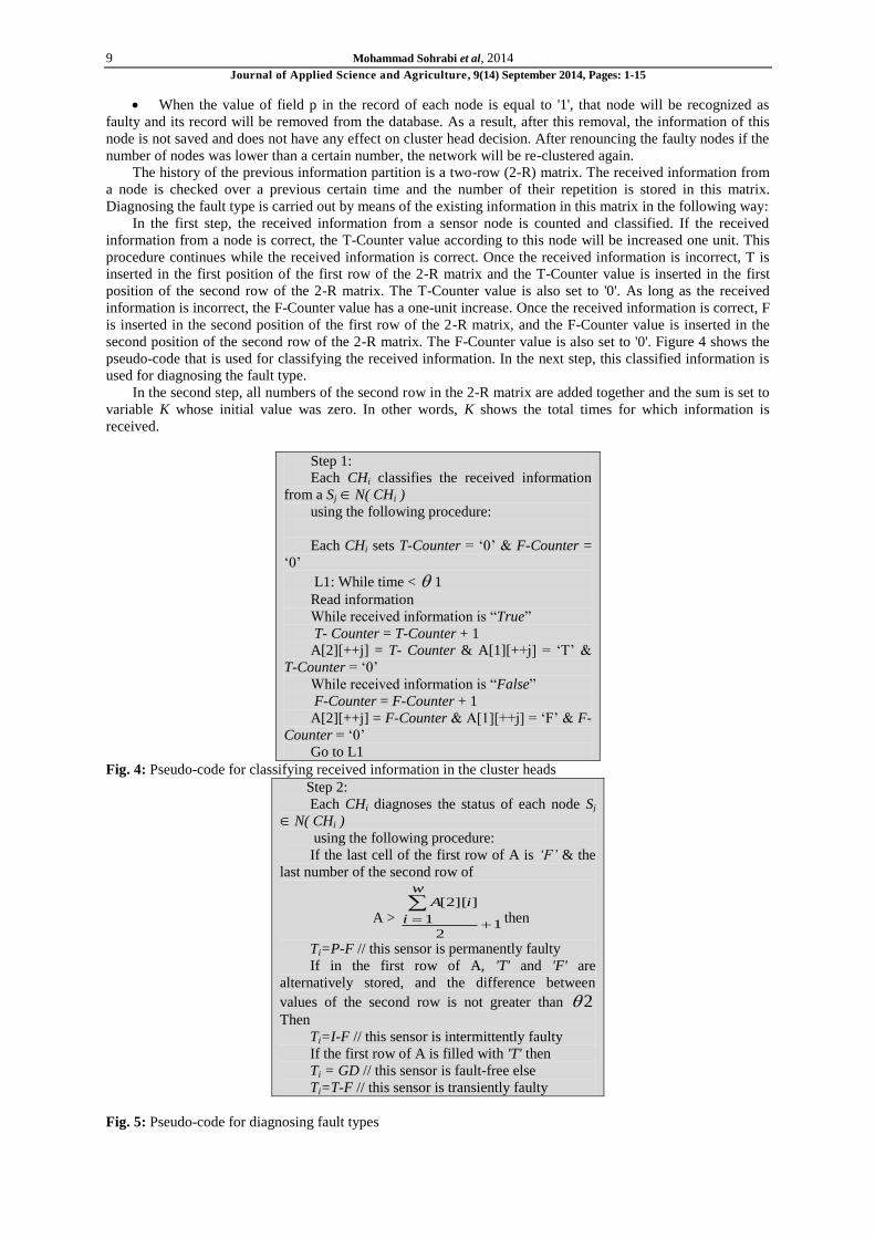
When the value of field p in the record of each node is equal to '1', that node will be recognized as

faulty and its record will be removed from the database. As a result, after this removal, the information of this

node is not saved and does not have any effect on cluster head decision. After renouncing the faulty nodes if the

number of nodes was lower than a certain number, the network will be re-clustered again.

The history of the previous information partition is a two-row (2-R) matrix. The received information from

a node is checked over a previous certain time and the number of their repetition is stored in this matrix.

Diagnosing the fault type is carried out by means of the existing information in this matrix in the following way:

In the first step, the received information from a sensor node is counted and classified. If the received

information from a node is correct, the ‌T-Counter‌ value according to this node will be increased one unit. This

procedure continues while the received information is correct. Once the received information is incorrect, T is

inserted in the first position of the first row of the 2-R matrix and the T-Counter value is inserted in the first

position of the second row of the 2-R matrix. The T-Counter value is also set to '0'. As long as the received

information is incorrect, the ‌F-Counter value has a one-unit increase. Once the received information is correct, F

is inserted in the second position of the first row of the 2-R matrix, and the F-Counter value is inserted in the

second position of the second row of the 2-R matrix. The F-Counter value is also set to '0'. Figure 4 shows the

pseudo-code that is used for classifying the received information. In the next step, this classified information is

used for diagnosing the fault type.

In the second step, all numbers of the second row in the 2-R matrix are added together and the sum is set to

variable K whose initial value was zero. In other words, K shows the total times for which information is

received.

Step 1:

Each CHi classifies the received information

from a Sj N( CHi )

using the following procedure:

Each CHi sets T-Counter = „0‟ & F-Counter =

„0‟

L1: While time < 1

Read information

While received information is “True”

T- Counter = T-Counter + 1

A[2][++j] = T- Counter & A[1][++j] = „T‟ &

T-Counter = „0‟

While received information is “False”

F-Counter = F-Counter + 1

A[2][++j] = F-Counter & A[1][++j] = „F‟ & F-

Counter = „0‟

Go to L1

Fig. 4: Pseudo-code for classifying received information in the cluster heads

Step 2:

Each CHi diagnoses the status of each node Sj

N( CHi )

using the following procedure:

If the last cell of the first row of A is ‘F’ & the

last number of the second row of

A > 1

2

1

]][2[

w

i

iA

then

Ti=P-F // this sensor is permanently faulty

If in the first row of A, 'T' and 'F' are

alternatively stored, and the difference between

values of the second row is not greater than 2

Then

Ti=I-F // this sensor is intermittently faulty

If the first row of A is filled with 'T' then

Ti = GD // this sensor is fault-free else

Ti=T-F // this sensor is transiently faulty

Fig. 5: Pseudo-code for diagnosing fault types



In the third step, the fault type is diagnosed as follows:

I) If the last cell of the first row of the 2-R matrix is F and the value of the last cell in the second row of

the 2-R matrix is equal to or greater than [K/2] +‌1, the fault type will be permanent and cannot be resolved.

Field P, related to this node, is set to '1'. According to the recovery algorithm, the record of this node will be

removed from the database of the sink or cluster head.

II) If the values of the second row of the 2-R matrix are alternately equal or there is a minor difference

between them, the fault type will be intermittent and the field I, related to this node, is set to '1'.

III) If only one position of the first row of the 2-R matrix is filled and it is T, it means that all the received

information is correct and the sink or the cluster head will recognize this sensor node as fault-free.

IV) Otherwise, the fault type will be transient and the field T, related to this node will be set to '1'.

Figure 5 shows the pseudo-code used for identifying the fault type.

Network Model:

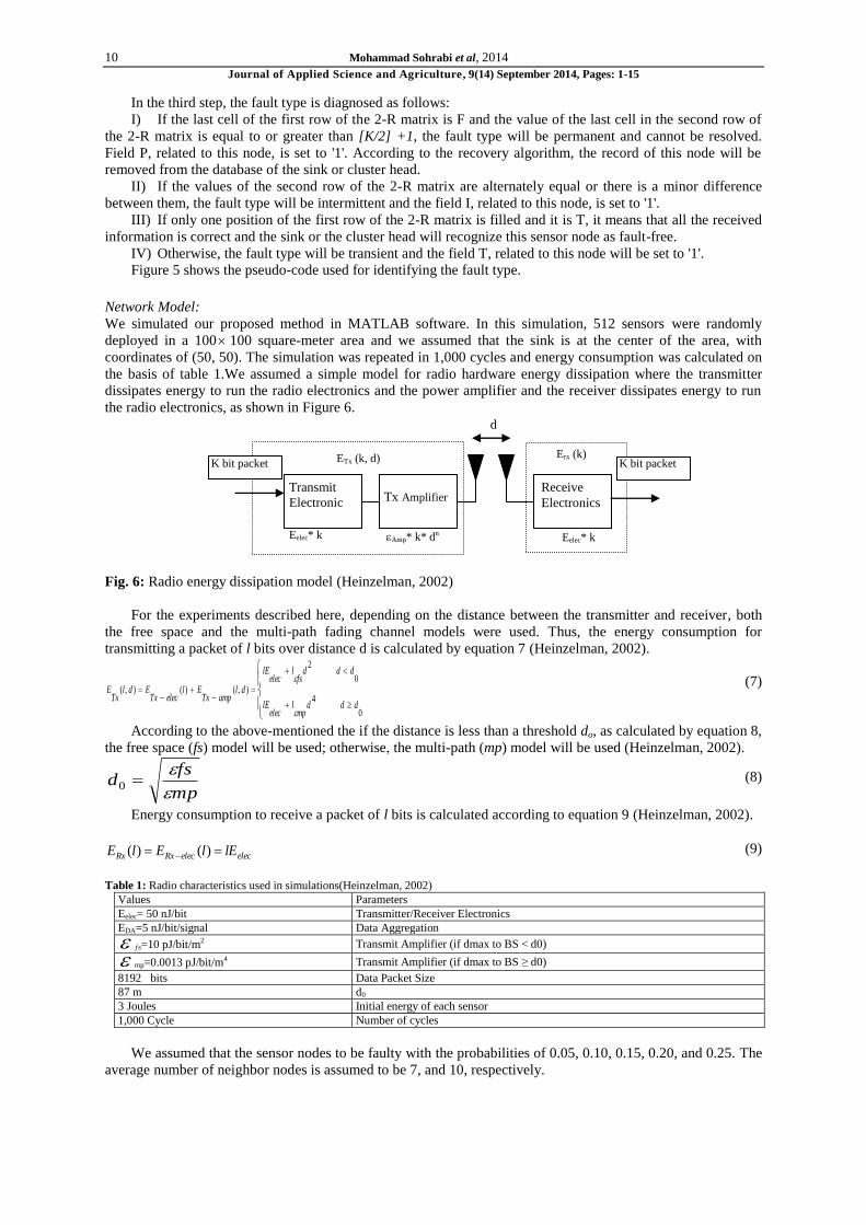
We simulated our proposed method in MATLAB software. In this simulation, 512 sensors were randomly

deployed in a 100 100 square-meter area and we assumed that the sink is at the center of the area, with

coordinates of (50, 50). The simulation was repeated in 1,000 cycles and energy consumption was calculated on

the basis of table 1.We assumed a simple model for radio hardware energy dissipation where the transmitter

dissipates energy to run the radio electronics and the power amplifier and the receiver dissipates energy to run

the radio electronics, as shown in Figure 6.

Fig. 6: Radio energy dissipation model (Heinzelman, 2002)

For the experiments described here, depending on the distance between the transmitter and receiver, both

the free space and the multi-path fading channel models were used. Thus, the energy consumption for

transmitting a packet of l bits over distance d is calculated by equation 7 (Heinzelman, 2002).

0

4

0

2

),()(),(

dddmp

lelec

lE

dddfs

lelec

lE

dlampTx

ElelecTx

EdlTx

E

(7)

According to the above-mentioned the if the distance is less than a threshold do, as calculated by equation 8,

the free space (fs) model will be used; otherwise, the multi-path (mp) model will be used (Heinzelman, 2002).

mp

fsd

0

(8)

Energy consumption to receive a packet of l bits is calculated according to equation 9 (Heinzelman, 2002).

elecelecRxRx lElElE )()( (9)

Table 1: Radio characteristics used in simulations(Heinzelman, 2002)

Values Parameters

Eelec= 50 nJ/bit Transmitter/Receiver Electronics

EDA=5 nJ/bit/signal Data Aggregation

ƒs=10 pJ/bit/m2 Transmit Amplifier (if dmax to BS < d0)

mp=0.0013 pJ/bit/m4 Transmit Amplifier (if dmax to BS ≥ d0)

8192 bits Data Packet Size

87 m d0

3 Joules Initial energy of each sensor

1,000 Cycle Number of cycles

We assumed that the sensor nodes to be faulty with the probabilities of 0.05, 0.10, 0.15, 0.20, and 0.25. The

average number of neighbor nodes is assumed to be 7, and 10, respectively.

Transmit

Electronic Tx Amplifier

K bit packet ETx (k, d)

Eelec* k

Receive

Electronics

Erx (k) K bit packet

Eelec* k

d

Amp* k* dn



Simulation Results and Evaluations:

We evaluated the efficiency of our proposed method in terms of Detection Accuracy (DA) and False Alarm

Rate (FAR) parameters with Lee and Chen algorithms. The DA is defined as the ratio of the number of detected

faulty nodes to the total number of faulty nodes while FAR is defined as the ratio of the number of fault-free

nodes that are detected as faulty node to the total number of fault-free nodes. On the other hand, suppose that

denotes the number of faulty sensors that are diagnosed as faulty in the network; thus, the correction accuracy

can be represented asnp

. Similarly, suppose that denotes the number of fault-free nodes that are diagnosed

as faulty. Thus the false alarm rate is represented as)1( Pn

(Gao, 2007).

Figures 7 and 8 show the simulation results for DA when the average numbers of neighboring nodes for

each node are 7 and, 10 respectively.

Fig. 7: DA of in the proposed method for W=7

Fig. 8: DA of the proposed method for W=10

If the probability of a node being faulty is 0.1 and each node has an average number of 7 neighbor nodes,

Lee and Chen algorithms will respectively have DA equal to 0.986 and 0.984 but the DA in the proposed

method will be 0.992. Thus, if the probability of a node being faulty is 0.25 Lee and Chen algorithms will

respectively have a DA equal to 0.975 and 0.97 but the DA in the proposed method will be 0.985. Similarly, as

shown in table 2, if each node has an average of 10 neighbor nodes and the probability of a node being faulty is

0.1, Lee and Chen algorithms will yield a DA which will be equal to 0.999 but the DA in the proposed method

will be 1. If the probability of a node being faulty is 0.25, Lee and Chen algorithms will respectively have DA a

equal to 0.993 and 0.991 but the DA in the proposed method will be 0.996. In general, when the probability of a

node being faulty increases, the DA in the proposed method will increases than that in Lee and Chen algorithms.

Table 2 shows the numerical values of the comparison results.



Table 2: DA in the proposed method, compared to Chen and Lee algorithms

P Algorithms

Chen Lee Proposed algorithm Chen Lee Proposed algorithm

0.05 0.996 0.998 0.999 1.0 1.0 1.0

0.1 0.984 0.986 0.992 0.999 0.999 1.0

0.15 0.983 0.985 0.992 0.998 0.998 0.999

0.2 0.982 0.984 0.991 0.997 0.998 0.998

0.25 0.97 0.975 0.985 0.991 0.993 0.996

W=7 W=10

Average number of neighbor nodes

Figures 9 and 10 show the comparison of the proposed method with Chen and Lee algorithms in terms of

FAR, when the average numbers of neighbor nodes are 7 and 10 for each node respectively.

Fig. 9: FAR of the proposed method for W=7

Fig. 10: FAR of the proposed method for W=10

If the probability of a node being faulty is 0.15 and each node has an average of 7 neighbor nodes, Lee and

Chen algorithms will respectively have FAR equal to 0 and 0.0001 but the FAR in the proposed method will be

0. Thus, if the probability of a node being faulty is 0.25, Lee and Chen algorithms will respectively have FAR

which are equal to 0.0018 and 0.0021 but the FAR in the proposed method will be 0.0014. Similarly, as shown

in table 3, when each node has an average of 10 neighbor nodes, and the probability of a node being faulty is

0.15, Lee and Chen algorithms will respectively have FAR equal to 0 and 0.0001 but the FAR of the proposed

method will be 0. If the probability of a node being faulty is 0.25, Lee and Chen algorithms will respectively

have FAR equal to 0.0012 and 0.0014 but FAR in the proposed method will be 0.0009. In general, when the

probability of a node being faulty increases, FAR in the proposed method will decrease more than those in Lee

and Chen algorithms. Table 3 shows the numerical values of the simulation results.

In Figure 11, the average remaining energy in the proposed algorithm and in Chen and Lee algorithms are

compared with each other. It is shown that in the initial rounds, the average energy of sensors in the proposed

method decreases faster than those in Chen and Lee algorithms. This is due to the fact that many messages will

be transmitted between sensor nodes in the clustering process and cluster head selection of the proposed method,

thus resulting in such a reduction. Given that query messages will be sent in the proposed method to reach a

definitive decision, energy consumption in the proposed method is greater than those in the other mentioned

methods. But approximately after 700 rounds, we see that the average amount of remaining energy in the



proposed method is higher than those in Chen and Lee algorithms. Therefore, at the end of 1,000 rounds, the

remaining energy in the proposed method will be greater than those of other algorithms.

Table 3: FAR in the proposed method, compared to Chen and Lee algorithms

P Algorithms

Chen Lee Proposed method Chen Lee Proposed method

0.05 0.0 0.0 0.0 0.0 0.0 0.0

0.1 0.0 0.0 0.0 0.0 0.0 0.0

0.15 0.0001 0.0 0.0 0.0001 0.0 0.0

0.2 0.0003 0.0001 0.0 0.0003 0.0001 0.0

0.25 0.0021 0.0018 0.0014 0.0014 0.0012 0.0009

W=7 W=10

Average number of neighbor nodes

Fig. 11: Energy consumption of the proposed method in comparison to Chen and Lee algorithms

Conclusion and Future Works:

Due to the failure of sensor nodes, fault tolerance in wireless sensor networks will diminish; thus, detecting

faulty nodes and eliminating them from a network are considered to be essential. In this paper, we proposed a

new method to solve the shortcomings of majority voting. The proposed method was also intended to detect

permanent faults in sensor nodes with a considerably high DA and low FAR as well as extracting them from the

network by an appropriate approach. The proposed method can tolerate transient and intermittent faults in

relation to sensor reading and communication so that performance degradation is negligible. To investigate the

efficiency of the proposed approach, we compared its efficiency with those of Chen and Lee algorithms.

Simulation results showed that the proposed method demonstrates better performance across parameters such as

DA and FAR, even when the number of faulty sensor nodes is high. Moreover, the evaluations in the present

paper showed that the proposed method reduces energy consumption and improves network life time and fault

tolerance. In the future, we can use a combination of this method with a learning automata technique for fault

detection and for increasing network fault tolerance.

REFERENCES

Abbasi, A.A., M. Younis, 2007. A survey on clustering algorithms for wireless sensor networks. Comput

Commun, 30: 2826-2841.

Akyildiz, I.F., W. Su, Y. Sankarasubramaniam, E. Cayirci, 2002. Wireless Sensor Networks: a survey.

Comput Netw, 38: 393-422.

Asim, M., H. Mokhtar, M. Merabti, 2008. A Fault Management Architecture for wireless sensor networks.

In: International Wireless Communications and Mobile Computing Conference (IWCM ‟08) Crete Island, Greece,

pp: 779-785.

Babaei, S.h., H. Jafarian, A. Hosseinalipour, 2011. A New Scheme for Detecting Faulty Sensor Nodes and

Excluding them from the Network. In: proceedings of Information and Managemnt Engineering, Springer link,

pp: 36-42.

Bandyopadhyay, S., E.J. Coyle, 2003. An energy efficient hierarchical clustering algorithm for wireless

sensor networks. In: Proceedings of the 22nd Annual Joint Conference of the IEEE Computer and

Communications Societies (INFOCOM ‟03), San Francisco, California, USA, pp: 1713-1723.

Chen, J., S. Kher, A. Somani, 2006. Distributed Fault Detection of Wireless Sensor Networks. In:

Proceedings of the 2006 workshop on Dependability issues in wireless ad hoc networks and sensor networks

(DIWANS ‟06) NY, USA, pp: 65-72.

Chenglin, Z.h., S. Xuebin, S. Songlin, J. Ting, 2011. Fault diagnosis of sensor by chaos particle swarm



optimization algorithm and support vector machine. Expert Syst Appl., 38: 9908-9912.

Chessa, S., P. Santi, 2002. Crash faults identification in wireless sensor networks. Comput Commun, 25:

1273-1282.

Choi, J.-Y., S.-J. Yim, Y.J. Huh, Y.-H. Choi, 2009. A Distributed Adaptive Scheme for Detecting Faults in

Wireless Sensor Networks. WSEAS Trans Commun, 8: 269-278.

Ding, M., D. Chen, K. Xing, X. Cheng, 2005. Localized fault-tolerant event boundary detection in sensor

networks. In: Proceeding of the 24th Annual Joint Conference of the IEEE Computer and Communications

Societies (INFOCOM ‟05) Miami, USA, pp: 902-913.

Ding, P., J. Holliday, A. Celik, 2005. Distributed energy efficient hierarchical clustering for wireless sensor

networks. In: Proceedings of the IEEE International Conference on Distributed Computing in Sensor Systems

(DCOSS ‟05), Marina Del Rey, CA, pp: 322-339.

Fedor, S., M. Collier, 2007. On the problem of energy efficiency of multi-hop vs one-hop routing in wireless

sensor networks. In: Proceedings of the 21st International Conference on Advanced Information Networking and

Applications Workshops (AINAW ‟2007), Niagara Falls, Canada, pp: 380-385.

Gangloff, W.C., 1974. Common Mode Failure Analysis. IEEE Trans, Power App. Syst., 94: 27-30.

Gao, J., Y. Xu, X. Li, 2007. Online Distributed Fault Detection of Sensor Measurements. Tsinghua Sci

Technol., 12: 192-196.

Gehrke, J., S. Madden, 2004. Query Processing in Sensor Networks. IEEE Pervasive Comput., 3: 46-55.

Guo, S., Z. Zhong, T. He, 2009. FIND: Faulty Node Detection for Wireless Sensor Networks. In:

Proceedings of the 7th ACM Conference on Embeded Networked Sensor Systems (SenSys ‟09), California,

USA., pp: 253-266.

Heinzelman, W.B., A.P. Chandrakasan, H. Balakrishnan, 2002. Application specific protocol architecture for

wireless microsensor networks. IEEE Trans; Wirel Commun., 1: 660-670.

Hsin, C., M. Liu, 2005. Self-monitoring of Wireless Sensor Networks. Comput Commun, 29: 462-476.

Huang, R., X. Qiu, L. Rui, 2011. Simple Random Sampling-Based Probe Station Selection for Fault

Detection in Wireless Sensor Networks. Sensors., 11: 3117-3134.

Hyun oh, S., O. Hong Ch., Y.-H. Choi, 2012. A Malicious and Malfunctioning Node Detection Scheme for

Wireless Sensor Networks. Wirel Sensor Netw, 4: 84-90.

Jiang, P., 2009. A New Method for Node Fault Detection in Wireless Sensor Networks. Sensors., 9: 1282-

1294.

Koushanfar, F., M. Potkonjak, A. Sangiovanni-Vincentalli, 2004. Fault Tolerance in Sensor Networks. In:

Ilyas M, Mahgoub I (ed) Handbook of Sensor Networks:Compact Wireless and Wired Sensing Systems,

CRC Press, Boca Raton, FL, USA., 36: 1-36.

Krunic, V., E. Trumpler, R. Han, 2007. NodeMD: Diagnosing Node-level faults in Remote Wireless Sensor

Networks. In:Proceedings of the 5th international conference on Mobile systems, applications and services

(MobiSys '07), San Juan, Puerto Rico, pp: 43-56.

Lai, Y., H. Chen, 2007. Energy-Efficient Fault-Tolerant Mechanism for Clustered Wireless Sensor Networks.

In: proceedings of 16th International Conference on Computer Communications and Networks (ICCCN ‟07)

Honolulu, Hawaii, USA, pp: 272-277.

Lee, J.-H., I.-B. Jung, 2010. Speedy Routing Recovery Protocol for Large Failure Tolerance in Wireless

Sensor Networks. Sensors, 10: 3389-3410.

Lee, M.-H., Y.-H. Choi, 2008. Fault detection of wireless sensor networks. Comput Commun., 31: 3469-

3475.

Luo, X., M. Dong, Y. Huang, 2006. On distributed fault-tolerant detection in wireless sensor networks. IEEE

Trans Comput., 55: 58-70.

Mahapatro, A., P.M. Khilar, 2012. Detection of Node Failure in Wireless Image Sensor Networks. ISRN

Sensor Netw.

Mahapatro, A., P.M. Khilar, 2011. Scalable Distributed Diagnosis Algorithm for Wireless Sensor Networks.

In: Proceedings of the Advances in Computing, Communication and Control, Springer link, pp: 400-405.

Rahmani, O. and A. Taherkhani, 2014. A method of data encryption in NOC, Journal of Applied Science and

Agriculture, 9(4): 1903-1906

Paoli, A., 2003. Fault Detection and Fault Tolerant Control for Distributed systems. Ph.D. thesis, University

of Bolonga.

Shell, J., S. Coupland, E. Goodyer, 2010. Fuzzy Data Fusion for Fault Detection in Wireless Sensor

Networks. In: Proceedings of the 10th Annual Workshop on Computational Intelligence (UKCI ‟10), London,

UK., pp: 1-6.

Ssu, K-F., Ch-H. Chou, H. Christine Jiau, W-T. Hu, 2002. Detection and diagnosis of data inconsistency

failures in wireless sensor networks. Comput Netw, 50: 1247-1260.

Warriach, E.U., K. Tei, T.A. Nguyen, M. Aiello, 2012. Fault detection in wireless sensor networks: a hybrid

approach. In: Proceedings of the 11th International Conference on Information Processing in Sensor Networks

http://www.sigmobile.org/mobisys/2007/index.html



(IPSN ‟12), Beijing, China, pp: 87-88.

Yick, J., B. Mukherjee, D. Ghosal, 2004. Wireless Sensor Network Survey. Comput Netw, 52: 2292-2330.

Younis, O., S. Fahmy, 2004. HEED: A Hybrid, Energy-Efficient, Distributed clustering approach for Ad Hoc

sensor networks. IEEE Trans. Mob Comput., 3: 366-379.

Farzin Salimi, Meysam EsmaeilZadeh Ashieni, 2014.Investigation on the effects of communications and

information's globalization on the process of education in Iran, Journal of Applied Science and Agriculture, 9(7):

2785-2794.

Sajad Varasteh and Ebrahim Abbasi, 2014. Study the effect of firm size on the relationship between

ownership concentration and information asymmetry, Advances in Environmental Biology, 8(9): 776-780.

Tabatabaei, S.A., A. Morovate and A. Soltanzadeh, 2014. Locating Defects in Composite Shells using Modal

Analysis , Advances in Environmental Biology, 8(6): 2130-2135.

Mitra Farsi, Narjes Shafiee Sarvestani, Sedigheh Hassanzade, Maryam Sharif, 2014. The Effect of Computer-

assisted Language Learning and E-learning on Vocabulary Learning, Journal of Applied Science and Agriculture,

9(7): 2749-2753.

journal of applied science and agriculture 2014/1-15.pdf · journal of applied science and...

Documents