jorunal article. parabolic solar trough

8/10/2019 Jorunal article. Parabolic solar trough

http://slidepdf.com/reader/full/jorunal-article-parabolic-solar-trough 1/7

Estimating intercept factor of a parabolic solar trough collector with newsupporting structure using off-the-shelf photogrammetric equipment

Silverio García-Cortés a, Antonio Bello-García b, Celestino Ordóñez a,c,⇑

a Dept. of Mining Exploitation, University of Oviedo, 33600 Mieres, Spainb Dept. of Industrial Manufacturing, University of Oviedo, 33203 Gijón, Spainc Dept. of Natural Resources, University of Vigo, 36211 Vigo, Spain

a r t i c l e i n f o

Article history:

Received 24 March 2011

Received in revised form 29 July 2011

Accepted 19 August 2011

Available online 21 September 2011

Keywords:

Close-range photogrammetry

Quality control

Parabolic trough collector

Solar concentrator

a b s t r a c t

When a new design for a solar collector is developed it is necessary to guarantee that its intercept factor is

good enough to produce the expected thermal jump. This factor is directly related with the fidelity of the

trough geometry with respect to its theoretical design shape. This paper shows the work carried out to

determine the real shape and the intercept factor of a new prototype of parabolic solar collector. Conver-

gent photogrammetry with off-the-shelf equipment was used to obtain a 3D point cloud that is simulta-

neously oriented in space and adjusted to a parabolic cylinder in order to calculate the deviations from

the ideal shape. Thenormal vectors at each point in theadjusted surface arecalculated and used to deter-

mine the intercept factor. Deviations between adjusted shape and the theoretical one suggest mounting

errors for some mirror facets, resulting in a global intercept factor slightly below the commonly accepted

limit for this type of solar collector.

2011 Elsevier Ltd. All rights reserved.

1. Introduction

Power generation through solar fields is starting to increase

strongly in Europe (especially in Spain) and the USA [1]. There is

also a big interest in sustainable energy supply all over the world

with special focus on USA, China and North Africa. Nine large com-

mercial scale plants were built in the Mojave Desert (California,

USA) during 1980s. Since then, interest in this technology seemed

to decline. Andasol 1, a 50 MW parabolic trough solar plant located

in Granada (southern Spain), began its construction in 2006. Today

there are 10 parabolic trough plants working in this country, ten

more are under construction and 26 more are planned [2]. In addi-

tion further projects with a capacity over 2000 MW are planned all

over the world mainly in the USA, China and North Africa [1].

A concentrating solar plant (CSP) using parabolic trough

collector technology (PTC) is composed of a large field of PTC, a heatexchanger block and a conventional turbine–generator system. So-

lar fields comprise rows of PTCaligned north–south which can track

sun direct radiation during the day (Fig. 1). Loops of parabolic

trough solar collectors with lengths about 600 m are used. These

loops are in turncomposed of smaller modules(150 m)whose basic

components are the 12 m long parabolic trough segments.

Parabolic trough collectors (PCC, parabolic cylindrical collector)

consist of a number of elementary large mirrors (28 mirrors, being

155 cm 170 cm each) forming a parabolic trough surface as per-

fect as possible. They transform the sun’s radiant energy into heatenergy, which is absorbed by a pipe of oil located on the focal line

of the parabolic cylinder. The oil temperature at the end of the so-

lar field must be about 400 C. This thermal energy is transferred to

water vapor in a heat exchanger that feeds a turbine for electricity

production.

Global thermal efficiency of parabolic trough collectors (PTC)

depend on several factors but geometric agreement to parabolic

profile design is the most important one and is the one considered

here. The objective of this article is to determine, for a PTC segment

with a new supporting structure design, the deviation of its shape

with respect to the theoretical one and estimate its intercept factor

(the fraction of the reflected radiation that is incident on the

absorbing surface of the receiver).

The paper is structured as follows. Section 2 provides a sum-mary of the factors that influence the thermal efficiency of a solar

collector. In Section 3, the procedure to obtain the geometry of a

PTC segment and its deviation from the theoretical shape is pre-

sented. Section 4 explains the methodology employed to estimate

the intercept coefficient of the PTC. In Section 5, results obtained

for the particular case analyzed are shown. Finally, we present

our conclusions.

2. Thermal efficiency of parabolic solar collectors

The instantaneous efficiency of a parabolic solar collector can be

expressed as a function of three parameters [3]:

0306-2619/$ - see front matter 2011 Elsevier Ltd. All rights reserved.doi:10.1016/j.apenergy.2011.08.032

⇑ Corresponding author. Address: E.P. Mieres, Calle Gonzalo Gutiérrez Quirós s/n,

33600 Mieres, Asturias, Spain. Tel.: +34 985458020; fax: +34 985458000.

E-mail addresses: [email protected], [email protected] (C. Ordóñez).

Applied Energy 92 (2012) 815–821

Contents lists available at SciVerse ScienceDirect

Applied Energy

j o u r n a l h o m e p a g e : w w w . e l s e v i e r . c o m / l o c a t e / a p e n e r g y

http://dx.doi.org/10.1016/j.apenergy.2011.08.032

mailto:[email protected]



http://www.sciencedirect.com/science/journal/03062619

http://www.elsevier.com/locate/apenergy

http://www.elsevier.com/locate/apenergy

http://www.sciencedirect.com/science/journal/03062619







gC ¼ f ðF R; U C ;g0Þ

The F R parameter measures the efficiency of the heat transmissionto the absorber fluid. U C quantify the thermal losses per unit of

the receiver surface area. This factor depends primarily on the

temperature difference between the collector and the environment.

Finally g0 is the optical efficiency which depends on solar beam

incidence angle (angle between the sun rays and the normal to

the aperture plane), the properties of the collector materials (mirror

reflectance, receiver cover transmittance, absorber tube absorp-

tance) and the optical errors.

Optical efficiency g0 of the collector can be studied indepen-

dently from the thermal parameters if we assume that the collector

material properties are invariant from temperature. In that case

optical efficiency varies with the incidence angle h, also with

effective transmittance–absorptance factor (sa)n and with inter-

cept factor at normal angle of incidence c (fraction of rays incident

upon the aperture that reach the receiver when the incidence angle

is zero [3]).

g0 ¼ K ðhÞðsaÞnc

In turn, the intercept factor is controlled by the geometric design of

the collector through the rim angle / (angle between the two ends

of the aperture geometry measured from the focal point in a trans-

versal section of the collector), random and non-random errors.

Random errors are due to the change in the apparent sun width,

rsun (the distribution of energy directed to the receiver, also called

sun shape), small and occasional sun tracking errors,rtrack, errors in

mirror specularity, rslope (defects in the reflective material) and

small scale slope errors, rslope (waviness of the mirrors). These

random errors can be modeled by a normal probability energy dis-

tribution where the total reflected energy standard deviation is [4].

rtot ¼ ffiffiffiffiffiffiffiffiffiffiffiffiffiffiffiffiffiffiffiffiffiffiffiffiffiffiffiffiffiffiffiffiffiffi ffiffiffiffiffiffiffiffiffiffiffiffiffiffiffiffiffiffiffiffiffiffiffiffiffiffiffiffiffir2

sun þ 4r2

slope þ r2

track þ r2

mirror

q Non-random errors can be categorized in three classes: the

misalignment of the receiver tube with respect the focus line of

the parabolic cylinder, misalignment of the trough with the sun

and the difference in the average shape of the collector with respect

to the parabolic section (profile errors). These non-random errors

can be caused by defective manufacturing or assembling, imperfect

tracking of sun and poor operation conditions (sand, dust or distor-

tion of the collector geometry caused by winds).

All these effects can be grouped in four parameters to model the

intercept factor at normal incidence angle [3]:

c ¼ f ðu;r;b; dÞ

The rim angle, /, takes into account the characteristics of the collec-

tor design,r models the effect of random errors (universal random

error parameter), b is the universal non-random angular errors

parameter and is modeled by the misalignment angle (angle be-

tween the central ray from the sun the normal to the aperture

plane), Finally d is the universal non-random error parameter

and takes into account for the profile errors and the misalignment

of the receiver with respect the focal line.

In our case, we measure a collector module fitted with a new

supporting design structure. This module has been assembled

alone for measurement purposes only and there is no receiver tube

installed. At this point of the process, manufacturer is only inter-

ested in testing the rigidity of the structure compared with the

mechanical design specifications. Thus we have measured the

module in vertical and horizontal positions to assess that the

new designed structure can maintain the parabolic shape for the

collector. Due to this special configuration of the collector, receiver

tube misalignment, angular non-random errors (misalignment of

collector with respect the sun) and random errors can be excluded

as influence factors. Incidence angle is also not affecting the inter-

cept factor at normal incidence. Consequently, only the profile er-

rors in the collectors are considered in this study.

Profile errors depend on the degree of adjustment for this set of

28 mirrors to the parabolic cylindrical geometry. Movements and

deflections of the supporting structure under its own weight and

under external forces like wind affect the geometry of the collec-

tors. Different support designs exist on the market [5]. Each new

design of the structure supporting the mirrors must be tested to

find if this design and the associated assembly process are able

to maintain the geometry within reasonable limits of solar ray con-

centration. Errors in mirror assembly and alignment influence the

efficiency of electricity production very much [6].

There are several situations where a collector must be geomet-

rically controlled. First, during mirror mounting in the assembly

facility [7], generally near the solar field location, where only the

supporting structure and mirrors are present. Second, when placed

on the solar field for the first time, to control surface deviationscaused during transportation and after receiver tube installation

[8]. Third, during normal operation to control evolution and stabil-

ity against winds and sun track movement [9,10].

In addition every new collector design must be controlled and

measured to ensure the supporting structure effectiveness and a

minimum intercept factor capability. Plataforma Solar Almeria

(PSA) [11] is one of the companies that carry out this assessment

by providing the appropriate certification to the company owning

the design.

3. PTC segment shape estimation with off the shelf

photogrammetric equipment

3.1. Collector targeting

Photogrammetric processes are based on the registration of ob-

ject points in several images taken from different positions [12,8].

3D coordinates of these points are then reconstructed from their

coordinates on images. For this reason, image coordinates of points

must be measured with high precision. Mirror surfaces are prob-

lematic because of their reflective behavior. The absence of natural

points must be solved using targets arranged on a collector surface.

These targets will be detected automatically during the photo-

grammetric work. The usual procedure is to attach a sheet of adhe-

sive vinyl on the surface, with a printed array of targets with

appropriate size and shape.

Target spacing and size depend on mean photographic capturedistance and target detection method implemented on the photo-

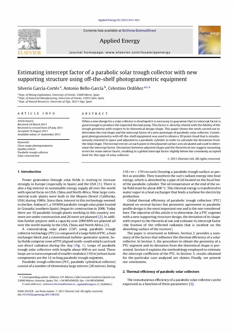
Fig. 1. A view of solar collector field in Extresol 1 solar plant (Spain).

816 S. García-Cortés et al. / Applied Energy 92 (2012) 815–821



grammetric software. In general, circular targets, printed or retro-

reflective ones, are recommended since automatic detection of cir-

cle centroid (which becomes an ellipse because of the perspective

projection of the photograph) is a process that can be carried out

accurately by the LSM (‘‘least squares matching’’) technique [12].

In this case, signal array has been designed and provided by Plata-

forma Solar Almería (PSA) staff [11]. The target array has been de-

signed to facilitate the triangulation process and spacing between

neighboring circular targets is 10 cm. Target diameter is 4 cm and

they must appear as about ten pixel size when used with adequate

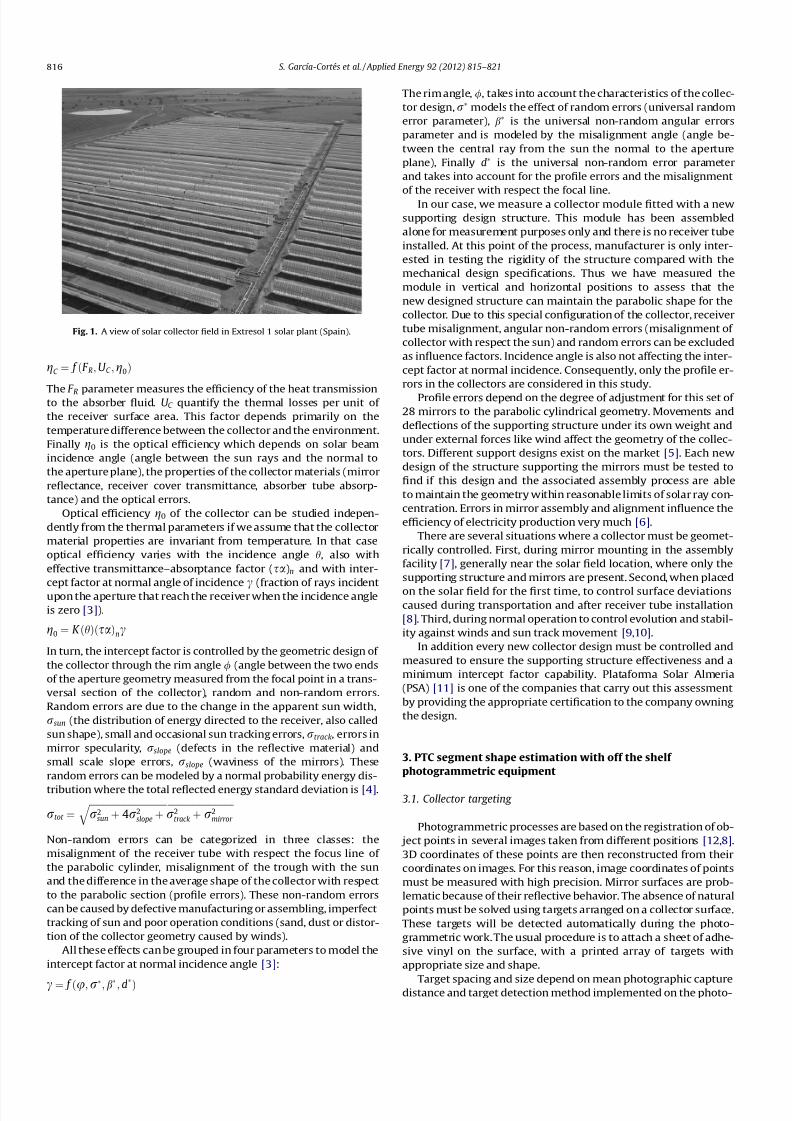
shooting distance and camera (sensor) resolution (Fig. 2).

In order to achieve a faster process, 14 coded targets were

evenly distributed over the collector surface (Fig. 2). These targets

are automatically recognized by the photogrammetric software

and automatically matched between images [13]. There were

about 7150 circular targets covering the collector surface. This high

number of signals is necessary to improve the reconstruction of the

trough surface by interpolation during the meshing procedure and

is not necessary in other studies which are not addressed to inter-

cept factor determination [8,14].

3.2. Photographic shooting and 3D processing

Classical photogrammetric technique requires a convergent

geometry of camera axis with respect to the subject [15]. More-

over, each point of the object must appear in at least two images.

Concentrator modeling has to be done in two different positions:

vertical and horizontal, to be aware of the geometry variation dur-

ing sun tracking. Being a large object (12 m long and 5.30 m open-

ing) the average distance from which the images have to be shot is

influenced by lens field angle, target size (on image) and accessibil-

ity. An off-the-shelf SLR camera with a standard 18–55 mm

lens was used. The camera and lens specifications can be seen in

Table 1.

In order to determine accurate camera model parameters (focal

length, principal point position and lens distortion parameters),the camera must be calibrated. Camera calibration can be carried

out by two different methods. The first method consists in taking

several photos convergent to a target grid specially designed for

that purpose. Different distances and camera format positions are

used to avoid coupling between internal parameters. This is a

well-known procedure [12,15] and was done by creating a special

camera calibration project inside Photomodeler 6 [16]. Second pos-

sibility for calibration is to solve a field calibration. In this case

internal geometry of camera-lens system is recovered using the

same set of photos used for object reconstruction. This method

takes into account possible instabilities which can appear during

shooting procedure in the field (principal distance and principal

point variations and others, due to switch on–off process of the

camera, thermal variations, camera shaking, etc.).

In our case we use the calibration parameters obtained in the

first method as a base values for the bundle adjustment of the full

block of photographs during the second procedure. This improves

the absorption of typical instabilities affecting this commercial

(off-the-shelf) camera. The basic calibration parameters are al-

lowed to change during bundle adjustment procedure implement-

ing the field calibration process mentioned above. Some other

precautions were adopted to try to get a fixed internal geometry:

deactivation of lens stabilization, optic zoom fixing and all photos

taken in wide angle zoom position (calibrated position).

Average shooting distance to the collector in a vertical position

was found tobe about 8 m for the nine images, and a little less (6 m

approx.) for horizontal position. This is caused by the height limit

that could be achieved with the existing hydraulic lifting platform.

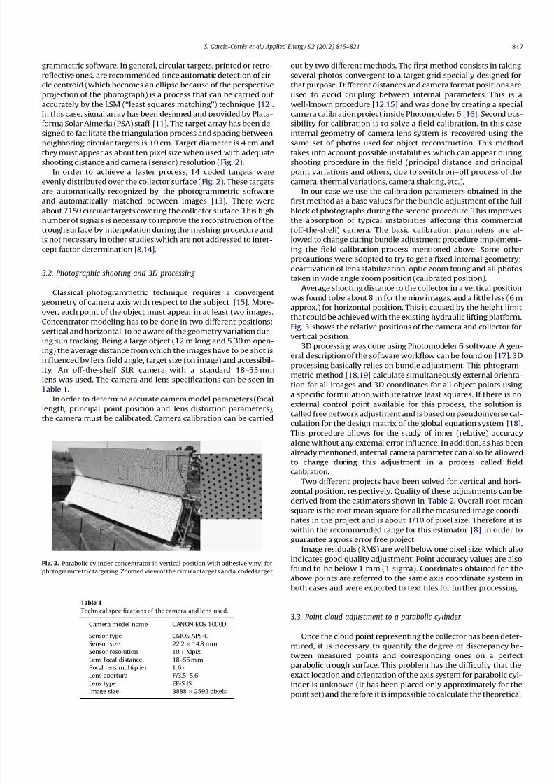
Fig. 3 shows the relative positions of the camera and collector for

vertical position.

3D processing was done using Photomodeler 6 software. A gen-

eral description of the software workflow can be found on [17]. 3D

processing basically relies on bundle adjustment. This phtogram-

metric method [18,19] calculate simultaneously external orienta-

tion for all images and 3D coordinates for all object points using

a specific formulation with iterative least squares. If there is no

external control point available for this process, the solution is

called free network adjustment and is based on pseudoinverse cal-culation for the design matrix of the global equation system [18].

This procedure allows for the study of inner (relative) accuracy

alone without any external error influence. In addition, as has been

already mentioned, internal camera parameter can also be allowed

to change during this adjustment in a process called field

calibration.

Two different projects have been solved for vertical and hori-

zontal position, respectively. Quality of these adjustments can be

derived from the estimators shown in Table 2. Overall root mean

square is the root mean square for all the measured image coordi-

nates in the project and is about 1/10 of pixel size. Therefore it is

within the recommended range for this estimator [8] in order to

guarantee a gross error free project.

Image residuals (RMS) are well below one pixel size, which alsoindicates good quality adjustment. Point accuracy values are also

found to be below 1 mm (1 sigma). Coordinates obtained for the

above points are referred to the same axis coordinate system in

both cases and were exported to text files for further processing.

3.3. Point cloud adjustment to a parabolic cylinder

Once the cloud point representing the collector has been deter-

mined, it is necessary to quantify the degree of discrepancy be-

tween measured points and corresponding ones on a perfect

parabolic trough surface. This problem has the difficulty that the

exact location and orientation of the axis system for parabolic cyl-

inder is unknown (it has been placed only approximately for thepoint set) and therefore it is impossible to calculate the theoretical

Fig. 2. Parabolic cylinder concentrator in vertical position with adhesive vinyl for

photogrammetric targeting. Zoomed view of the circular targets and a coded target.

Table 1

Technical specifications of the camera and lens used.

Camera model name CANON EOS 1000D

Sensor type CMOS APS-C

Sensor size 22.2 14.8 mm

Sensor resolution 10.1 Mpix

Lens focal distance 18–55 m m

Focal lens multiplier 1.6

Lens apertura F/3.5–5.6

Lens type EF-S IS

Image size 3888 2592 pixels

S. García-Cortés et al./ Applied Energy 92 (2012) 815–821 817



coordinates corresponding to each point following the basicequation:

z ¼ y2

2 p ð1Þ

being y and z coordinates of the points over the parabolic cylinder

surface and p, a constant, describing the parabolic shape of trans-

versal sections.

To take this problem into account, a coordinate transformation

in space (rigid body) is included in the model. Its parameters will

account for the misalignment and the translation between real

and theoretical reference systems. This will allow the ideal para-

bolic cylinder to rotate, and change position during adjustment,

(a change of scale is not allowed) to fit, under the least square cri-

teria, the measured point cloud. The mathematical formulation of

the model is based on the geometric definition of a parabola. Dis-

tance from any point in the parabolic cylinder surface to the focus

line must be equal the distance from the same point to the direc-

trix plane.

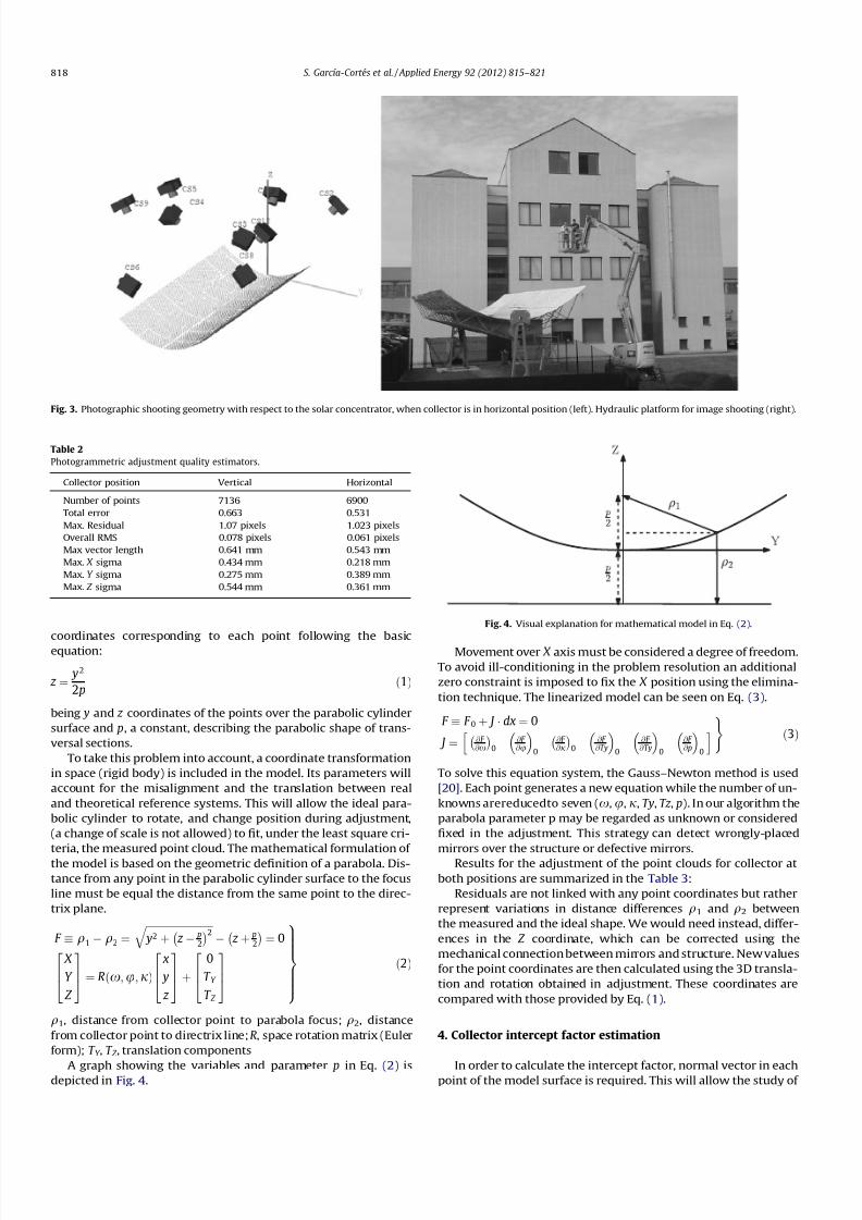
F q1 q

2 ¼

ffiffiffiffiffiffiffiffiffiffiffiffiffiffiffiffiffiffiffiffiffiffiffiffiffiffiffi y2 þ z p

2

2q z þ p

2

¼ 0

X

Y

Z

264

375 ¼ Rðx;u;jÞ

x

y

z

264

375þ

0

T Y

T Z

264

375

9>>>>>=>>>>>;

ð2Þ

q1, distance from collector point to parabola focus; q2, distance

from collector point to directrix line; R, space rotation matrix (Euler

form); T Y , T Z , translation components

A graph showing the variables and parameter p in Eq. (2) isdepicted in Fig. 4.

Movement over X axis must be considered a degree of freedom.

To avoid ill-conditioning in the problem resolution an additional

zero constraint is imposed to fix the X position using the elimina-

tion technique. The linearized model can be seen on Eq. (3).

F F 0 þ J dx ¼ 0

J ¼ @ F @ x

0

@ F @ u

0

@ F @ j

0

@ F @ Ty

0

@ F @ Ty

0

@ F @ p

0

h i) ð3Þ

To solve this equation system, the Gauss–Newton method is used

[20]. Each point generates a new equation while the number of un-

knowns arereducedto seven (x,u, j, Ty, Tz , p). In our algorithm the

parabola parameter p may be regarded as unknown or considered

fixed in the adjustment. This strategy can detect wrongly-placed

mirrors over the structure or defective mirrors.

Results for the adjustment of the point clouds for collector at

both positions are summarized in the Table 3:

Residuals are not linked with any point coordinates but rather

represent variations in distance differences q1 and q2 between

the measured and the ideal shape. We would need instead, differ-

ences in the Z coordinate, which can be corrected using the

mechanical connection between mirrors and structure. New values

for the point coordinates are then calculated using the 3D transla-

tion and rotation obtained in adjustment. These coordinates are

compared with those provided by Eq. (1).

4. Collector intercept factor estimation

In order to calculate the intercept factor, normal vector in eachpoint of the model surface is required. This will allow the study of

Fig. 3. Photographic shooting geometry with respect to the solar concentrator, when collector is in horizontal position (left). Hydraulic platform for image shooting (right).

Table 2

Photogrammetric adjustment quality estimators.

Collector position Vertical Horizontal

Number of points 7136 6900

Total error 0.663 0.531

Max. Residual 1.07 pixels 1.023 pixels

Overall RMS 0.078 pixels 0.061 pixels

Max vector length 0.641 mm 0.543 mm

Max. X sigma 0.434 mm 0.218 mm

Max. Y sigma 0.275 mm 0.389 mm

Max. Z sigma 0.544 mm 0.361 mm

Fig. 4. Visual explanation for mathematical model in Eq. (2).




reflected rays. A mesh was constructed using meshing functions on

MATLAB, which in turn uses the CGAL [21] free library. The

meshing algorithm used was Delaunay in 2D, over the xy plane

projection.

Normal vectors to the centroid of each triangle are calculated

and used to determine the reflected rays over the collector at any

point. Solar rays coming from a direction parallel to the longitudi-

nal symmetry plane of the collector will be reflected symmetrically

with respect to normal. For perfect geometry, all rays should be re-

flected on the focal line of parabolic trough. Deviation from this

behavior reduces the optical efficiency of solar collector [9]. Under

the hypothesis of a perfect collector alignment with solar ray direc-

tion, reflected ray direction must be computed. To avoid confusions

and to speed up the process we pose this problem under a vector

formulation (Fig. 5).

Distance between oil pipe center (over focal parabolic line) and

the reflected sun ray on P will define if the ray hits the pipe

(dFQ < R pipe) or not. We can calculate the position vector for the foot

of the minimum distance segment (Q ) between reflected ray and

oil pipe with:

OQ ¼ OP þ r

kr kt r

t r ¼ t r kr k

ð4Þ

where r is the reflected ray direction vector and t r stands for the

projection of t vector over r (being t the vector connecting the sur-

face point P with the focal point F) (Fig. 5, left). Vector t can be eas-

ily obtained for each surface point.

Vector r can be found as follows (Fig. 5, right):

r ¼ z þ 2 w ¼ z þ 2ðz v Þ

v ¼ N z N

N z ¼ N z ¼ cos a

ð5Þ

From Eqs. (4) and (5) can be noted the main importance of precise

determination for the Z axis. The point cloud space orientation

implicitly defines this axis. Thus also determine the accuracy of re-

flected ray directions.

The intercept factor measures the percentage of rays that inter-

sect the absorber tube against the total of all the reflected rays. For

such calculation the diameter of the absorber must be considered.

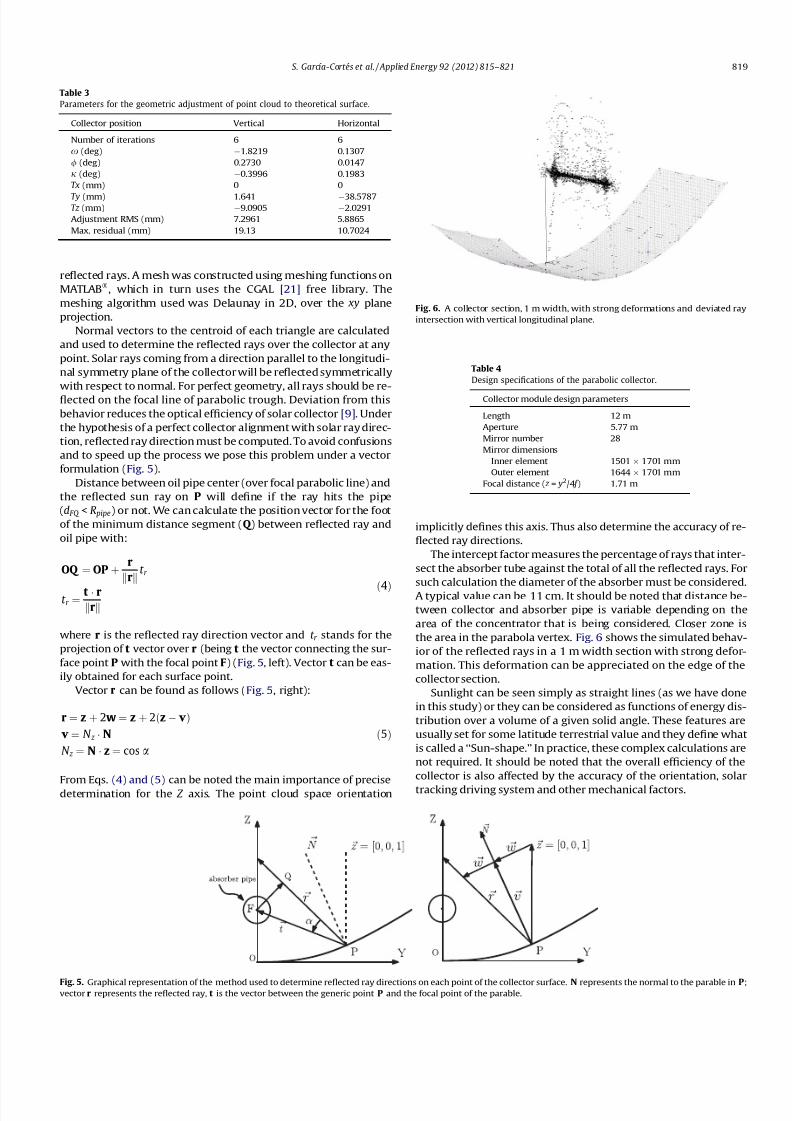
A typical value can be 11 cm. It should be noted that distance be-

tween collector and absorber pipe is variable depending on the

area of the concentrator that is being considered. Closer zone is

the area in the parabola vertex. Fig. 6 shows the simulated behav-

ior of the reflected rays in a 1 m width section with strong defor-

mation. This deformation can be appreciated on the edge of the

collector section.

Sunlight can be seen simply as straight lines (as we have done

in this study) or they can be considered as functions of energy dis-

tribution over a volume of a given solid angle. These features are

usually set for some latitude terrestrial value and they define what

is called a ‘‘Sun-shape.’’ In practice, these complex calculations are

not required. It should be noted that the overall efficiency of the

collector is also affected by the accuracy of the orientation, solar

tracking driving system and other mechanical factors.

Table 3

Parameters for the geometric adjustment of point cloud to theoretical surface.


Number of iterations 6 6

x (deg) 1.8219 0.1307

/ (deg) 0.2730 0.0147

j (deg) 0.3996 0.1983

Tx (mm) 0 0

Ty (mm) 1.641 38.5787Tz (mm) 9.0905 2.0291

Adjustment RMS (mm) 7.2961 5.8865

Max. residual (mm) 19.13 10.7024

Fig. 5. Graphical representation of the method used to determine reflected ray directions on each point of the collector surface. N represents the normal to the parable in P;vector r represents the reflected ray, t is the vector between the generic point P and the focal point of the parable.

Fig. 6. A collector section, 1 m width, with strong deformations and deviated ray

intersection with vertical longitudinal plane.

Table 4

Design specifications of the parabolic collector.

Collector module design parameters

Length 12 m

Aperture 5.77 m

Mirror number 28

Mirror dimensions

Inner element 1501 1701 mm

Outer element 1644 1701 mm

Focal distance ( z = y2/4 f ) 1.71 m

S. García-Cortés et al. / Applied Energy 92 (2012) 815–821 819



5. Results and discussion

The methodology explained in Sections 2 and 3 was applied to

the geometrical study of a PTC designed and constructed for a

Spanish company. This collector module has been equipped with

a redesign supporting structure. It is based on EuroTrough design

(ET150 model) [22,23].

The technical specifications of the PTC used in this study aresummarized in Table 4.

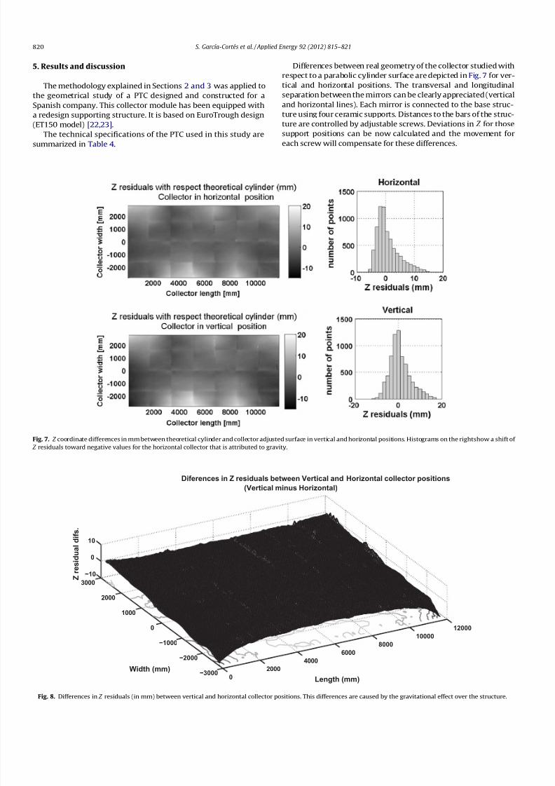
Differences between real geometry of the collector studied with

respect to a parabolic cylinder surface are depicted in Fig. 7 for ver-

tical and horizontal positions. The transversal and longitudinal

separation between the mirrors can be clearly appreciated (vertical

and horizontal lines). Each mirror is connected to the base struc-

ture using four ceramic supports. Distances to the bars of the struc-

ture are controlled by adjustable screws. Deviations in Z for those

support positions can be now calculated and the movement for

each screw will compensate for these differences.

Fig. 7. Z coordinate differences in mm between theoretical cylinder and collector adjusted surface in vertical and horizontal positions. Histograms on the rightshow a shift of

Z residuals toward negative values for the horizontal collector that is attributed to gravity.

0

2000

4000

6000

8000

10000

12000

−3000

−2000

−1000

0

1000

2000

3000

−10

0

10

Length (mm)

Diferences in Z residuals between Vertical and Horizontal collector positions

(Vertical minus Horizontal)

Width (mm)

Z r

e s i d u a

l d i f s .

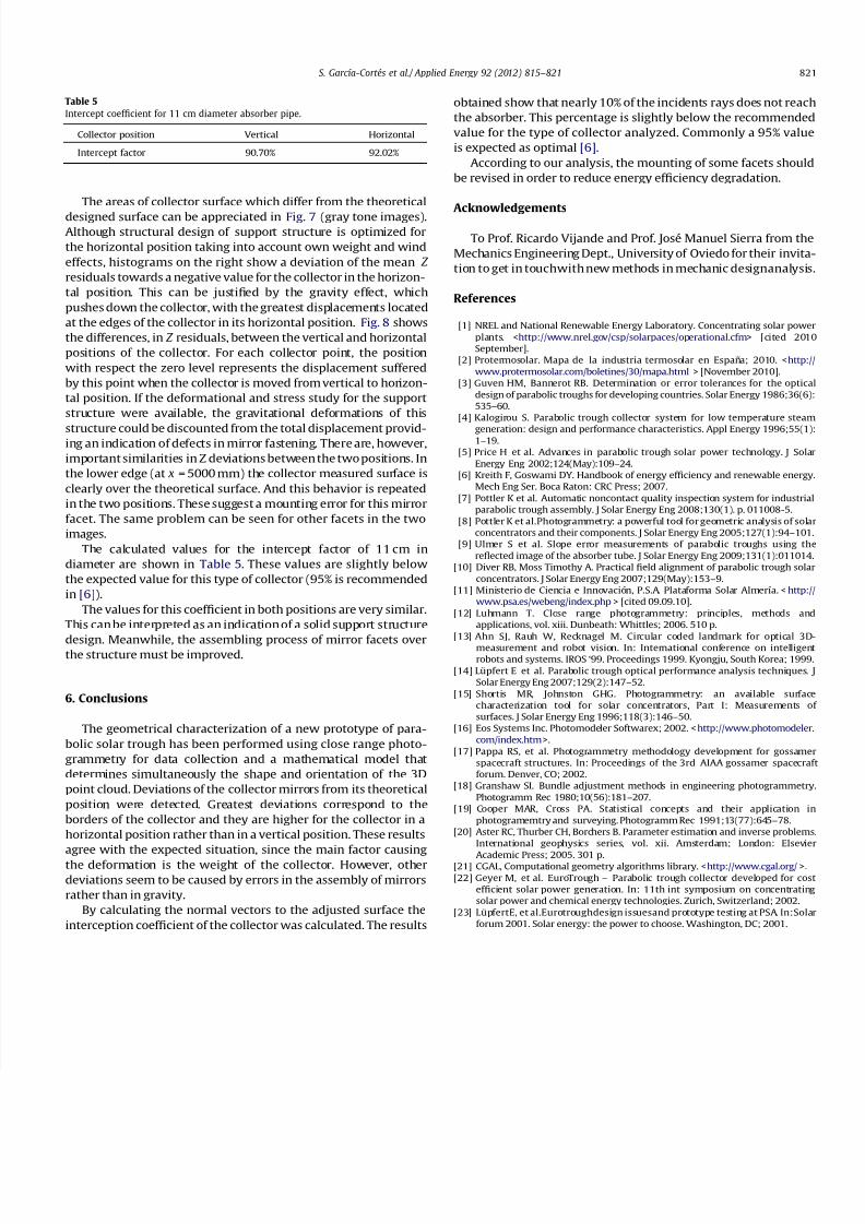
Fig. 8. Differences in Z residuals (in mm) between vertical and horizontal collector positions. This differences are caused by the gravitational effect over the structure.




The areas of collector surface which differ from the theoretical

designed surface can be appreciated in Fig. 7 (gray tone images).Although structural design of support structure is optimized for

the horizontal position taking into account own weight and wind

effects, histograms on the right show a deviation of the mean Z

residuals towards a negative value for the collector in the horizon-

tal position. This can be justified by the gravity effect, which

pushes down the collector, with the greatest displacements located

at the edges of the collector in its horizontal position. Fig. 8 shows

the differences, in Z residuals, between the vertical and horizontal

positions of the collector. For each collector point, the position

with respect the zero level represents the displacement suffered

by this point when the collector is moved from vertical to horizon-

tal position. If the deformational and stress study for the support

structure were available, the gravitational deformations of this

structure could be discounted from the total displacement provid-ing an indication of defects in mirror fastening. There are, however,

important similarities in Z deviations between the two positions. In

the lower edge (at x = 5000 mm) the collector measured surface is

clearly over the theoretical surface. And this behavior is repeated

in the two positions. These suggest a mounting error for this mirror

facet. The same problem can be seen for other facets in the two

images.

The calculated values for the intercept factor of 11 cm in

diameter are shown in Table 5. These values are slightly below

the expected value for this type of collector (95% is recommended

in [6]).

The values for this coefficient in both positions are very similar.

This can be interpreted as an indication of a solid support structure

design. Meanwhile, the assembling process of mirror facets overthe structure must be improved.

6. Conclusions

The geometrical characterization of a new prototype of para-

bolic solar trough has been performed using close range photo-

grammetry for data collection and a mathematical model that

determines simultaneously the shape and orientation of the 3D

point cloud. Deviations of the collector mirrors from its theoretical

position were detected. Greatest deviations correspond to the

borders of the collector and they are higher for the collector in a

horizontal position rather than in a vertical position. These results

agree with the expected situation, since the main factor causing

the deformation is the weight of the collector. However, other

deviations seem to be caused by errors in the assembly of mirrors

rather than in gravity.

By calculating the normal vectors to the adjusted surface the

interception coefficient of the collector was calculated. The results

obtained show that nearly 10% of the incidents rays does not reach

the absorber. This percentage is slightly below the recommended

value for the type of collector analyzed. Commonly a 95% value

is expected as optimal [6].

According to our analysis, the mounting of some facets should

be revised in order to reduce energy efficiency degradation.

Acknowledgements

To Prof. Ricardo Vijande and Prof. José Manuel Sierra from the

Mechanics Engineering Dept., University of Oviedo for their invita-

tion to get in touchwith new methods in mechanic designanalysis.

References

[1] NREL and National Renewable Energy Laboratory. Concentrating solar power

plants. <http://www.nrel.gov/csp/solarpaces/operational.cfm> [cited 2010

September].

[2] Protermosolar. Mapa de la industria termosolar en España; 2010. <http://

www.protermosolar.com/boletines/30/mapa.html > [November 2010].

[3] Guven HM, Bannerot RB. Determination or error tolerances for the optical

design of parabolic troughs for developing countries. Solar Energy 1986;36(6):

535–60.

[4] Kalogirou S. Parabolic trough collector system for low temperature steam

generation: design and performance characteristics. Appl Energy 1996;55(1):1–19.

[5] Price H et al. Advances in parabolic trough solar power technology. J Solar

Energy Eng 2002;124(May):109–24.

[6] Kreith F, Goswami DY. Handbook of energy efficiency and renewable energy.

Mech Eng Ser. Boca Raton: CRC Press; 2007.

[7] Pottler K et al. Automatic noncontact quality inspection system for industrial

parabolic trough assembly. J Solar Energy Eng 2008;130(1). p. 011008-5.

[8] Pottler K et al.Photogrammetry: a powerful tool for geometric analysis of solar

concentrators and their components. J Solar Energy Eng 2005;127(1):94–101.

[9] Ulmer S et al. Slope error measurements of parabolic troughs using the

reflected image of the absorber tube. J Solar Energy Eng 2009;131(1):011014.

[10] Diver RB, Moss Timothy A. Practical field alignment of parabolic trough solar

concentrators. J Solar Energy Eng 2007;129(May):153–9.

[11] Ministerio de Ciencia e Innovación, P.S.A. Plataforma Solar Almería. <http://

www.psa.es/webeng/index.php > [cited 09.09.10].

[12] Luhmann T. Close range photogrammetry: principles, methods and

applications, vol. xiii. Dunbeath: Whittles; 2006. 510 p.

[13] Ahn SJ, Rauh W, Recknagel M. Circular coded landmark for optical 3D-

measurement and robot vision. In: International conference on intelligent

robots and systems. IROS ‘99. Proceedings 1999. Kyongju, South Korea; 1999.

[14] Lüpfert E et al. Parabolic trough optical performance analysis techniques. J

Solar Energy Eng 2007;129(2):147–52.

[15] Shortis MR, Johnston GHG. Photogrammetry: an available surface

characterization tool for solar concentrators, Part I: Measurements of

surfaces. J Solar Energy Eng 1996;118(3):146–50.

[16] Eos Systems Inc. Photomodeler Softwarex; 2002. <http://www.photomodeler.

com/index.htm>.

[17] Pappa RS, et al. Photogrammetry methodology development for gossamer

spacecraft structures. In: Proceedings of the 3rd AIAA gossamer spacecraft

forum. Denver, CO; 2002.

[18] Granshaw SI. Bundle adjustment methods in engineering photogrammetry.

Photogramm Rec 1980;10(56):181–207.

[19] Cooper MAR, Cross PA. Statistical concepts and their application in

photogramemtry and surveying. Photogramm Rec 1991;13(77):645–78.

[20] Aster RC, Thurber CH, Borchers B. Parameter estimation and inverse problems.

International geophysics series, vol. xii. Amsterdam; London: Elsevier

Academic Press; 2005. 301 p.[21] CGAL, Computational geometry algorithms library. <http://www.cgal.org/ >.

[22] Geyer M, et al. EuroTrough – Parabolic trough collector developed for cost

efficient solar power generation. In: 11th int symposium on concentrating

solar power and chemical energy technologies. Zurich, Switzerland; 2002.

[23] LüpfertE, et al.Eurotroughdesign issuesand prototype testing at PSA. In:Solar

forum 2001. Solar energy: the power to choose. Washington, DC; 2001.

Table 5

Intercept coefficient for 11 cm diameter absorber pipe.


Intercept factor 90.70% 92.02%

S. García-Cortés et al./ Applied Energy 92 (2012) 815–821 821

http://www.nrel.gov/csp/solarpaces/operational.cfm

http://www.protermosolar.com/boletines/30/mapa.html


http://www.psa.es/webeng/index.php


http://www.photomodeler.com/index.htm


http://www.cgal.org/

http://www.cgal.org/







http://www.nrel.gov/csp/solarpaces/operational.cfm

jorunal article. parabolic solar trough

Documents