jordan canonical form: theory and practicegtsat/collection/morgan claypool... · abstract jordan...
TRANSCRIPT

Jordan Canonical FormTheory and Practice

Synthesis Lectures onMathematics and Statistics
EditorSteven G. Krantz, Washington University, St. Louis
Jordan Canonical Form: Theory and PracticeSteven H. Weintraub2009
The Geometry of Walker ManifoldsMiguel Brozos-Vázquez, Eduardo García-Río, Peter Gilkey, Stana Nikcevic, Rámon Vázquez-Lorenzo2009
An Introduction to Multivariable MathematicsLeon Simon2008
Jordan Canonical Form: Application to Differential EquationsSteven H. Weintraub2008
Statistics is Easy!Dennis Shasha, Manda Wilson2008
A Gyrovector Space Approach to Hyperbolic GeometryAbraham Albert Ungar2008

Copyright © 2009 by Morgan & Claypool
All rights reserved. No part of this publication may be reproduced, stored in a retrieval system, or transmitted inany form or by any means—electronic, mechanical, photocopy, recording, or any other except for brief quotations inprinted reviews, without the prior permission of the publisher.
Jordan Canonical Form: Theory and Practice
Steven H. Weintraub
www.morganclaypool.com
ISBN: 9781608452507 paperbackISBN: 9781608452514 ebook
DOI 10.2200/S00218ED1V01Y200908MAS006
A Publication in the Morgan & Claypool Publishers seriesSYNTHESIS LECTURES ON MATHEMATICS AND STATISTICS
Lecture #6Series Editor: Steven G. Krantz, Washington University, St. Louis
Series ISSNSynthesis Lectures on Mathematics and StatisticsPrint 1938-1743 Electronic 1938-1751
Jordan Canonical FormTheory and Practice
Steven H. WeintraubLehigh University
SYNTHESIS LECTURES ON MATHEMATICS AND STATISTICS #6
CM& cLaypoolMorgan publishers&
ABSTRACTJordan Canonical Form (JCF ) is one of the most important, and useful, concepts in linear algebra.The JCF of a linear transformation, or of a matrix, encodes all of the structural information aboutthat linear transformation, or matrix. This book is a careful development of JCF. After beginningwith background material, we introduce Jordan Canonical Form and related notions: eigenvalues,(generalized) eigenvectors, and the characteristic and minimum polynomials. We decide the ques-tion of diagonalizability, and prove the Cayley–Hamilton theorem. Then we present a careful andcomplete proof of the fundamental theorem: Let V be a finite-dimensional vector space over the fieldof complex numbers C, and let T : V −→ V be a linear transformation. Then T has a Jordan CanonicalForm. This theorem has an equivalent statement in terms of matrices: Let A be a square matrix withcomplex entries. Then A is similar to a matrix J in Jordan Canonical Form, i.e., there is an invertible ma-trix P and a matrix J in Jordan Canonical Form with A = PJP −1. We further present an algorithmto find P and J , assuming that one can factor the characteristic polynomial of A. In developing thisalgorithm we introduce the eigenstructure picture (ESP) of a matrix, a pictorial representation thatmakes JCF clear. The ESP of A determines J , and a refinement, the labelled eigenstructure picture(�ESP) of A, determines P as well. We illustrate this algorithm with copious examples, and providenumerous exercises for the reader.
KEYWORDSJordan Canonical Form, characteristic polynomial, minimum polynomial, eigenvalues,eigenvectors, generalized eigenvectors, diagonalizability, Cayley–Hamilton theorem,eigenstructure picture

To my brother Jeffrey and my sister Sharon

ix
Contents
Preface . . . . . . . . . . . . . . . . . . . . . . . . . . . . . . . . . . . . . . . . . . . . . . . . . . . . . . . . . . . . . . . . . . . . . . . . . . xi
1 Fundamentals on Vector Spaces and Linear Transformations . . . . . . . . . . . . . . . . . . . . . . . . . . 1
1.1 Bases and Coordinates . . . . . . . . . . . . . . . . . . . . . . . . . . . . . . . . . . . . . . . . . . . . . . . . . . . . . . 1
1.2 Linear Transformations and Matrices . . . . . . . . . . . . . . . . . . . . . . . . . . . . . . . . . . . . . . . . . 4
1.3 Some Special Matrices . . . . . . . . . . . . . . . . . . . . . . . . . . . . . . . . . . . . . . . . . . . . . . . . . . . . . . 8
1.4 Polynomials in T and A . . . . . . . . . . . . . . . . . . . . . . . . . . . . . . . . . . . . . . . . . . . . . . . . . . . .11
1.5 Subspaces, Complements, and Invariant Subspaces . . . . . . . . . . . . . . . . . . . . . . . . . . . .13
2 The Structure of a Linear Transformation . . . . . . . . . . . . . . . . . . . . . . . . . . . . . . . . . . . . . . . . . . 17
2.5 Eigenvalues, Eigenvectors, and Generalized Eigenvectors . . . . . . . . . . . . . . . . . . . . . .17
2.2 The Minimum Polynomial . . . . . . . . . . . . . . . . . . . . . . . . . . . . . . . . . . . . . . . . . . . . . . . . . 23
2.3 Reduction to BDBUTCD Form . . . . . . . . . . . . . . . . . . . . . . . . . . . . . . . . . . . . . . . . . . . . .26
2.4 The Diagonalizable Case . . . . . . . . . . . . . . . . . . . . . . . . . . . . . . . . . . . . . . . . . . . . . . . . . . . 31
2.5 Reduction to Jordan Canonical Form . . . . . . . . . . . . . . . . . . . . . . . . . . . . . . . . . . . . . . . . 33
2.6 Exercises . . . . . . . . . . . . . . . . . . . . . . . . . . . . . . . . . . . . . . . . . . . . . . . . . . . . . . . . . . . . . . . . . 40
3 An Algorithm for Jordan Canonical Form and Jordan Basis . . . . . . . . . . . . . . . . . . . . . . . . . . 43
3.1 The ESP of a Linear Transformation . . . . . . . . . . . . . . . . . . . . . . . . . . . . . . . . . . . . . . . . 43
3.2 The Algorithm for Jordan Canonical Form . . . . . . . . . . . . . . . . . . . . . . . . . . . . . . . . . . .48
3.3 The Algorithm for a Jordan Basis . . . . . . . . . . . . . . . . . . . . . . . . . . . . . . . . . . . . . . . . . . . 53
3.4 Examples . . . . . . . . . . . . . . . . . . . . . . . . . . . . . . . . . . . . . . . . . . . . . . . . . . . . . . . . . . . . . . . . . 56
3.5 Exercises . . . . . . . . . . . . . . . . . . . . . . . . . . . . . . . . . . . . . . . . . . . . . . . . . . . . . . . . . . . . . . . . . 75
A Answers to odd-numbered exercises . . . . . . . . . . . . . . . . . . . . . . . . . . . . . . . . . . . . . . . . . . . . . . . 83
A.1 Answers to Exercises–Chapter 2 . . . . . . . . . . . . . . . . . . . . . . . . . . . . . . . . . . . . . . . . . . . . 83
A.2 Answers to Exercises–Chapter 3 . . . . . . . . . . . . . . . . . . . . . . . . . . . . . . . . . . . . . . . . . . . . 88

x CONTENTSNotation . . . . . . . . . . . . . . . . . . . . . . . . . . . . . . . . . . . . . . . . . . . . . . . . . . . . . . . . . . . . . . . . . . . . . . . . 93
Index . . . . . . . . . . . . . . . . . . . . . . . . . . . . . . . . . . . . . . . . . . . . . . . . . . . . . . . . . . . . . . . . . . . . . . . . . . . 95
PrefaceJordan Canonical Form (JCF ) is one of the most important, and useful, concepts in linear
algebra. The JCF of a linear transformation, or of a matrix, encodes all of the structural informationabout that linear transformation, or matrix. This book is a careful development of JCF.
In Chapter 1 of this book we present necessary background material. We expect that most,though not all, of the material in this chapter will be familiar to the reader.
In Chapter 2 we define Jordan Canonical Form and prove the following fundamentaltheorem: Let V be a finite-dimensional vector space over the field of complex numbers C, and letT : V −→ V be a linear transformation. Then T has a Jordan Canonical Form. This theorem hasan equivalent statement in terms of matrices: Let A be a square matrix with complex entries. ThenA is similar to a matrix J in Jordan Canonical Form. Along the way to the proof we introduceeigenvalues and (generalized) eigenvectors, and the characteristic and minimum polynomials of alinear transformation (or matrix), all of which play a key role. We also examine the special case ofdiagonalizability and prove the Cayley–Hamilton theorem.
The main result of Chapter 2 may be restated as: Let A be a square matrix with complexentries. Then there is an invertible matrix P and a matrix J in Jordan Canonical Form withA = PJP −1. In Chapter 3 we present an algorithm to find P and J , assuming that one canfactor the characteristic polynomial of A. In developing this algorithm we introduce the idea ofthe eigenspace picture (ESP) of A, which determines J , and a refinement, the labelled eigenspacepicture (�ESP) of A, which determines P as well.We illustrate this algorithm with copious examples.
Our numbering system in this text is fairly standard. Theorem 1.2.3 is the third numberedresult in Section 2 of Chapter 1.
We provide many exercises for the reader to gain facility in applying these concepts andin particular in finding the JCF of matrices. As is customary in texts, we provide answers to theodd-numbered exercises here. Instructors may contact me at [email protected] and I will supplyanswers to all of the exercises.
Steven H. WeintraubDepartment of Mathematics, Lehigh UniversityBethlehem, PA 18015 USAJuly 2009


1
C H A P T E R 1
Fundamentals on Vector Spacesand Linear Transformations
Throughout this book, all vector spaces will be assumed to be finite-dimensional vector spaces overthe field C of complex numbers.
We use, without further ado, the Fundamental Theorem of Algebra: Let f (x) = anxn +
an−1xn−1 + . . . + a1x + a0 be a polynomial of degree n with complex coefficients. Then f (x) =
an(x − r1)(x − r2) · · · (x − rn) for some complex numbers r1, r2, . . ., rn (the roots of the polynomial).
1.1 BASES AND COORDINATESIn this section, we discuss some of the basic facts on bases for vector spaces, and on coordinates forvectors.
First, we recall the definition of a basis.
Definition 1.1.1. Let V be a vector space and let B = {v1, . . . , vn} be a set of vectors of V . ThenB is a basis of V if it satisfies the following two conditions:
(1) B spans V , i.e., any vector v in V can be written as v = c1v1 + . . . + cnvn for some scalarsc1, . . . , cn; and
(2) B is linearly independent, i.e., the only solution of 0 = c1v1 + . . . + cnvn is the trivialsolution c1 = . . . = cn = 0. �Lemma 1.1.2. Let V be a vector space and let B = {v1, . . . , vn} be a set of vectors in V . Then B is abasis of V if and only if any vector v in V can be written as v = c1v1 + . . . + cnvn in a unique way.
Proof. First suppose that any vector v in V can be written as v = c1v1 + . . . + cnvn in aunique way. Then, in particular, it can be written as v = c1v1 + . . . + cnvn, so B spans V . Also, wecertainly have 0 = 0v1 + . . . + 0vn, so if this is the only way to write the 0 vector, when we write0 = c1v1 + . . . + cnvn we must have c1 = . . . = cn = 0.
Conversely, let B be a basis of V . Then, since B spans V , we can certainly write any vectorv in V in the form v = c1v1 + . . . + cnvn. Thus it remains to show that this can only be done inone way. So suppose that we also have v = c′
1v1 + . . . + c′nvn. Then we have 0 = v − v = (c1 −
c′1)v1 + . . . + (cn − c′
n)vn. By linear independence, we must have c1 − c′1 = . . . = cn − c′
n = 0, i.e.,c′
1 = c1, . . . , c′n = cn, and so we have uniqueness.
This lemma leads to the following definition.

2 CHAPTER 1. FUNDAMENTALS ON VECTOR SPACES AND LINEAR TRANSFORMATIONS
Definition 1.1.3. Let V be a vector space and let B = {v1, . . . , vn} be a basis of V . Let v be a vectorin V and write v = c1v1 + . . . + cnvn. Then the vector
[v]B =⎡⎢⎣
c1...
cn
⎤⎥⎦
is the coordinate vector of v in the basis B. �Remark 1.1.4. In particular, we may take V = C
n and consider the standard basis En = {e1, . . . , en}where
ei =
⎡⎢⎢⎢⎢⎢⎢⎢⎢⎣
0...
010...
⎤⎥⎥⎥⎥⎥⎥⎥⎥⎦
,
with 1 in the ith position, and 0 elsewhere. (We will often abbreviate En by E when there is nopossibility of confusion.)
Then, if
v =
⎡⎢⎢⎢⎢⎢⎣
c1
c2...
cn−1
cn
⎤⎥⎥⎥⎥⎥⎦
,
we see that
v = c1
⎡⎢⎢⎢⎢⎢⎣
10...
00
⎤⎥⎥⎥⎥⎥⎦
+ . . . + cn
⎡⎢⎢⎢⎢⎢⎣
00...
01
⎤⎥⎥⎥⎥⎥⎦
= c1e1 + . . . + cnen,
so we then see that
[v]En =
⎡⎢⎢⎢⎢⎢⎣
c1
c2...
cn−1
cn
⎤⎥⎥⎥⎥⎥⎦
.
(In other words, a vector in Cn “looks like” itself in the standard basis.) �

1.1. BASES AND COORDINATES 3
We have the following two properties of coordinates.
Lemma 1.1.5. Let V be a vector space and let B = {v1, . . . , vn} be any basis of V .(1) If v = 0 is the 0 vector in V , then [v]B = 0 is the 0 vector in C
n.(2) If v = vi , then [v]B = ei .
Proof. We leave this as an exercise for the reader.
Proposition 1.1.6. Let V be a vector space and let B = {v1, . . . , vn} be any basis of V .(1) For any vectors v1 and v2 in V , [v1 + v2]B = [v1]B + [v2]B.(2) For any vector v1 in V and any scalar c, [cv1]B = c[v1]B.(3) For any vector w in C
n, there is a unique vector v in V with [v]B = w.
Proof. We leave this as an exercise for the reader.
What is essential to us is the ability to compare coordinates in different bases. To that end,we have the following theorem.
Theorem 1.1.7. Let V be a vector space, and let B = {v1, . . . , vn} and C = {w1, . . . , wn} be two basesof V . Then there is a unique matrix PC←B with the property that, for any vector v in V ,
[v]C = PC←B[v]B.
This matrix is given by
PC←B =[[v1]C
∣∣∣∣ [v2]C∣∣∣∣ . . .
∣∣∣∣ [vn]C].
Proof. Let us first check that the given matrix P = PC←B has the desired property.To this end,let us first consider v = vi for some i. Then, as we have seen in Lemma 1.1.5 (2), [v]B = ei . By theproperties of matrix multiplication, Pei is the ith column of P , which by the definition of P is [vi]C .Thus in this case, we indeed have [v]C = P [v]C , as claimed. Now consider a general vector v. Then
on the one hand, by the definition of coordinates, if v = c1v1 + . . . + cnvn then [v]B = u =⎡⎢⎣
c1...
cn
⎤⎥⎦.
By Proposition 1.1.6 (1) and (2), we then have that [v]C = c1[v]C + . . . + cn[v]C , while on theother hand, by the definition of matrix multiplication, this is precisely Pu = P [v]B. Thus we have[v]C = P [v]C for every vector.
It remains only to show that P is the unique matrix with this property. Thus, suppose wehave another matrix P ′ with this property. To this end, let u be any vector in C
n. Then, by Proposi-tion 1.1.6 (3), there is a vector v in V with [v]B = u. Then we have [v]C = Pu and [v]C = P ′u, soP ′u = Pu. Since u is arbitrary, the only way this can happen is if P ′ = P .
Again, this theorem leads to a definition.
4 CHAPTER 1. FUNDAMENTALS ON VECTOR SPACES AND LINEAR TRANSFORMATIONS
Definition 1.1.8. The matrix PC←B is the change-of-basis matrix from the basis B to the basis C. �The change-of-basis matrix has the following properties.
Proposition 1.1.9. Let V be a vector space and let B, C, and D be any three bases of V . Then:(1) PB←B = I , the identity matrix.(2) PD←B = PD←CPC←B.(3) PC←B is invertible and (PC←B)−1 = PB←C .
Proof. (1) Certainly [v]B = I [v]B for every vector v in V , so by the uniqueness of the change-of-basis matrix, we must have PB←B = I .
(2) Using the fact that matrix multiplication is associative, we have
(PD←CPC←B)[v]B = PD←C(PC←B[v]B) = PD←C[v]C = [v]Dfor every vector v in V , so, again by the uniqueness of the change-of-basis matrix, we must havePD←B = PD←CPC←B.
(3) Setting D = B and using parts (1) and (2) we have that I = PB←B = PB←CPC←B.Similarly, we have that I = PC←C = PC←BPB←C , and hence these two matrices are inverses ofeach other.
We have just seen, in Proposition 1.1.9 (3), that every change-of-basis matrix is invertible. Infact, every invertible matrix occurs as a change-of-basis matrix, as we see from the next Proposition.
Proposition 1.1.10. Let P be any invertible n-by-n matrix. Then there are bases B and C of V = Cn
with PC←B = P .
Proof. Write P as
P =[p1
∣∣∣∣ p2
∣∣∣∣ . . .
∣∣∣∣ pn
].
Let B = {p1, p2, . . . , pn}. Since P is invertible, B is a basis of Cn. Let C = E be the standard
basis of V = Cn. We saw in Example 1.1.4 that [v]E = v for any vector v in V . In particular, this is
true for v = pi , for each i. But then, by Theorem 1.1.7,
PE←B =[[p1]E
∣∣∣∣ [p2]E∣∣∣∣ . . .
∣∣∣∣ [pn]E]
=[p1
∣∣∣∣ p2
∣∣∣∣ . . .
∣∣∣∣ pn
]= P,
as claimed.
1.2 LINEAR TRANSFORMATIONS AND MATRICESIn this section, we introduce linear transformations and their matrices.
First, we recall the definition of a linear transformation.

1.2. LINEAR TRANSFORMATIONS AND MATRICES 5
Definition 1.2.1. Let V and W be vector spaces. A linear transformation T is a function T : V −→W satisfying the following two properties:
(1) T (v1 + v2) = T (v1) + T (v2) for any two vectors v1 and v2 in V ; and(2) T (cv1) = c(v1) for any vector v1 in V and any scalar c. �A linear transformation has the following important property.
Lemma 1.2.2. Let V and W be vector spaces, and let B = {v1, . . . , vn} be any basis of V . Then a lineartransformation T : V −→ W is determined by {T (v1), . . . ,T (vn)}, which may be specified arbitrarily.
Proof. Suppose we are given T (vi) = wi for each i. Choose any vector v in V . Then, byLemma 1.1.2, v can be written uniquely as v = ∑
civi , and then, by the properties of a lineartransformation, T (v) = T (
∑civi) = ∑
ciT (vi) = ∑ciwi is determined.
On the other hand, suppose we choose any {w1, . . . , wn}. We define T as follows: First we setT (vi) = wi for each i. Then any vector v can be written as v = ∑
civi , so we set T (v) = ∑ciwi .
This gives us a well-defined function as there is only one such way to write v. It remains to check thatthe function T defined in this way is a linear transformation, and we leave that to the reader.
Here is one of the most important ways of constructing linear transformations.
Lemma 1.2.3. Let A be an m-by-n matrix and let TA : Cn → C
m be defined by TA(v) = Av. ThenTA(v) is a linear transformation.
Proof. This follows directly from properties of matrix multiplication: TA(v1 + v2) = A(v1 +v2) = Av1 + Av2 = TA(v1) + TA(v2) and TA(cv1) = A(cv1) = c(Av1) = cTA(v1).
In fact, once we choose bases, any linear transformation between finite-dimensional vectorspaces is given by multiplication by a matrix.
Theorem 1.2.4. Let V and W be vector spaces and let T : V −→ W be a linear transformation. LetB = {v1, . . . , vn} be a basis of V and let B = {w1, . . . , wm} be a basis of W . Then there is a uniquematrix [T ]C←B such that, for any vector v in V ,
[T (v)]C = [T ]C←B[v]B.
Furthermore, the matrix [T ]C←B is given by
[T ]C←B =[[T (v1)]C
∣∣∣∣ [T (v2)]C∣∣∣∣ . . .
∣∣∣∣ [T (vn)]C].
Proof. Let A be the given matrix. Consider any element vi of the basis B. Then [vi]B = ei ,and so TA([vi]B) = TA([ei]) = Aei is the ith column of A, which by the definition of the matrixA is [T (vi)]C . Thus, we have verified that [T (vi)]C = [T ]C←B[vi]B for each element of the basisB. Since this is true on a basis, it must be true for every element v of V , again using the factthat we can write every element v of V uniquely as v = c1v1 + . . . + cnvn. (Compare the proof ofTheorem 1.1.7.)

6 CHAPTER 1. FUNDAMENTALS ON VECTOR SPACES AND LINEAR TRANSFORMATIONS
Thus the matrix A has the property we have claimed. It remains to show that it is the uniquematrix with this property. Suppose we had another matrix A′ with the same property.Then we wouldhave A[v]B = [T (v)]C = A′[v]B for every v in V . Since for any vector u in C
n there is a vector v
with [v]B = u, we see that Au = A′u for every vector u in Cn, so we must have A′ = A. (Again
compare the proof of Theorem 1.1.7.)
Similarly, this theorem leads to a definition.
Definition 1.2.5. Let V and W be vector spaces and let T : V −→ V be a linear transformation.Let B = {v1, . . . , vn} be a basis of V and let B = {w1, . . . , wm} be a basis of W . Let [T ]C←B bethe matrix defined in Theorem 1.2.4. Then [T ]C←B is the matrix of the linear transformation Tfrom the basis B to the basis C. �Remark 1.2.6. In particular, we may take V = C
n and W = Cm, and consider the standard bases
En of V and Em of W . Let A be an m-by-n square matrix and write A =[a1
∣∣∣∣ a2
∣∣∣∣ . . .
∣∣∣∣ an
]. If TA
is the linear transformation given by TA(v) = Av, then
[TA]Em←En =[[TA(e1)]Em
∣∣∣∣ [TA(e2)]Em
∣∣∣∣ . . .
∣∣∣∣ [TA(en)]Em
]
=[[Ae1]Em
∣∣∣∣ [Ae2]Em
∣∣∣∣ . . .
∣∣∣∣ [Aen]Em
]
=[[a1]Em
∣∣∣∣ [a2]Em
∣∣∣∣ . . .
∣∣∣∣ [an]Em
]
=[a1
∣∣∣∣ a2
∣∣∣∣ . . .
∣∣∣∣ an
]
= A.
(In other words, the linear transformation given by multiplication by a matrix “looks like” that samematrix from one standard basis to another.) �
There is a very important special case of Definition 1.2.5, when T is a linear transformationfrom the vector space V to itself. In this case, we may choose the basis C to just be the basis B. Wecan also simplify the notation, as in this case, we do not need to record the same basis twice.
Definition 1.2.7. Let V be a vector space and let T : V −→ V be a linear transformation. LetB = {v1, . . . , vn} be a basis of V . Let [T ]B = [T ]B←B be the matrix defined in Theorem 1.2.4.Then [T ]B is the matrix of the linear transformation T in the basis B. �
What is essential to us is the ability to compare matrices of linear transformations in differentbases. To that end, we have the following theorem. (Compare Theorem 1.1.7.)
Theorem 1.2.8. Let V be a vector space, and let B = {v1, . . . , vn} and C = {w1, . . . , wn} be any twobases of V . Let PC←B be the change-of-basis matrix form B to C. Then, for any linear transformation

1.2. LINEAR TRANSFORMATIONS AND MATRICES 7
T : V −→ V ,
[T ]C = PC←B[T ]BPB←C= PC←B[T ]B(PC←B)−1
= (PB←C)−1[T ]BPB←C .
Proof. Let v be any vector in V . We compute:
(PC←B[T ]BPB←C)([v]C) = (PC←B[T ]B)(PB←C[v]C)
= (PC←B[T ]B)([v]B)
= PC←B([T ]B[v]B)
= PC←B[T (v)]B= [T (v)]C .
But, by definition, [T ]C is the unique matrix with the property that [T ]C([v]C) = [T (v)]Cfor every v in V .Thus these two matrices must be the same, yielding the first equality in the statementof the theorem. The second and third equalities then follow from Proposition 1.1.9 (3).
Again, this theorem leads to a definition.
Definition 1.2.9. Two square matrices A and B are similar if there is an invertible matrix P withA = PBP −1. A is said to be obtained from B by conjugation by P . The matrix P is called anintertwining matrix of A and B, or is said to intertwine A and B. �Remark 1.2.10. Note that if A = PBP −1, so that A is obtained from B by conjugation by P ,or equivalently that P intertwines A and B, then B = P −1AP , so that B is obtained from A byconjugation by P −1, or equivalently that P −1 intertwines B and A. �
Theorem 1.2.8 tells us that if A and B are matrices of the same linear transformation T withrespect to two bases of V , then A and B are similar. In fact, any pair of similar matrices arises in thisway. (Compare Proposition 1.1.10.)
Proposition 1.2.11. Let A and B be any two similar n-by-n matrices. Then there is a linear transfor-mation T : C
n −→ Cn and bases B and C of C
n such that [T ]B = A and [T ]C = B.
Proof. Let A = PBP −1, or, equivalently, B = P −1AP . Let T be the linear transformationT = TA. Let B be the basis of C
n whose elements are the columns of P −1, and let C = E be thestandard basis of C
n. Then, by Remark 1.2.6, [T ]E = A, and then, by Theorem 1.2.8, [T ]B =P −1AP = B.
Remark 1.2.12. This point is so important that it is worth specially emphasizing: Two matrices A
and B are similar if and only if they are the matrices of the same linear transformation T in twobases. �
8 CHAPTER 1. FUNDAMENTALS ON VECTOR SPACES AND LINEAR TRANSFORMATIONS
1.3 SOME SPECIAL MATRICESIn this section, we present a small menagerie of matrices of special forms. These matrices aresimpler than general matrices, and will be important for us to consider in the sequel.
All matrices we consider here are square matrices.
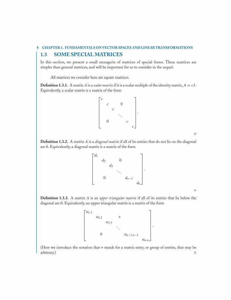
Definition 1.3.1. A matrix A is a scalar matrix if it is a scalar multiple of the identity matrix,A = cI .Equivalently, a scalar matrix is a matrix of the form
⎡⎢⎢⎢⎢⎢⎢⎢⎣
c
c 0c
. . .
0 c
c
⎤⎥⎥⎥⎥⎥⎥⎥⎦
.
�Definition 1.3.2. A matrix A is a diagonal matrix if all of its entries that do not lie on the diagonalare 0. Equivalently, a diagonal matrix is a matrix of the form
⎡⎢⎢⎢⎢⎢⎢⎢⎣
d1
d2 0d3
. . .
0 dn−1
dn
⎤⎥⎥⎥⎥⎥⎥⎥⎦
.
�Definition 1.3.3. A matrix A is an upper triangular matrix if all of its entries that lie below thediagonal are 0. Equivalently, an upper triangular matrix is a matrix of the form
⎡⎢⎢⎢⎢⎢⎢⎢⎣
a1,1
a2,2 ∗a3,3
. . .
0 an−1,n−1
an,n
⎤⎥⎥⎥⎥⎥⎥⎥⎦
.
(Here we introduce the notation that ∗ stands for a matrix entry, or group of entries, that may bearbitrary.) �
1.3. SOME SPECIAL MATRICES 9
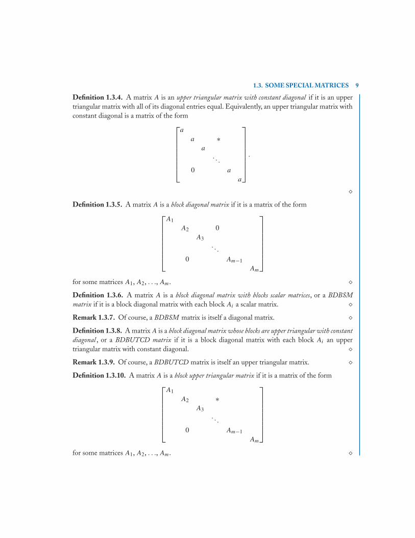
Definition 1.3.4. A matrix A is an upper triangular matrix with constant diagonal if it is an uppertriangular matrix with all of its diagonal entries equal. Equivalently, an upper triangular matrix withconstant diagonal is a matrix of the form
⎡⎢⎢⎢⎢⎢⎢⎢⎣
a
a ∗a
. . .
0 a
a
⎤⎥⎥⎥⎥⎥⎥⎥⎦
.
�Definition 1.3.5. A matrix A is a block diagonal matrix if it is a matrix of the form
⎡⎢⎢⎢⎢⎢⎢⎢⎣
A1
A2 0A3
. . .
0 Am−1
Am
⎤⎥⎥⎥⎥⎥⎥⎥⎦
for some matrices A1, A2, . . ., Am. �Definition 1.3.6. A matrix A is a block diagonal matrix with blocks scalar matrices, or a BDBSMmatrix if it is a block diagonal matrix with each block Ai a scalar matrix. �Remark 1.3.7. Of course, a BDBSM matrix is itself a diagonal matrix. �Definition 1.3.8. A matrix A is a block diagonal matrix whose blocks are upper triangular with constantdiagonal , or a BDBUTCD matrix if it is a block diagonal matrix with each block Ai an uppertriangular matrix with constant diagonal. �Remark 1.3.9. Of course, a BDBUTCD matrix is itself an upper triangular matrix. �Definition 1.3.10. A matrix A is a block upper triangular matrix if it is a matrix of the form
⎡⎢⎢⎢⎢⎢⎢⎢⎣
A1
A2 ∗A3
. . .
0 Am−1
Am
⎤⎥⎥⎥⎥⎥⎥⎥⎦
for some matrices A1, A2, . . ., Am. �
10 CHAPTER 1. FUNDAMENTALS ON VECTOR SPACES AND LINEAR TRANSFORMATIONS
You could easily (or perhaps not so easily) imagine why we would want to study the abovekinds of matrices, as they are simpler than arbitrary matrices and occur more or less naturally. Ourlast two kinds of matrices are ones you would certainly not come up with offhand, but turn out to bevitally important ones. Indeed, these are precisely the matrices we are heading towards. It will takeus a lot of work to get there, but it is easy for us to simply define them now and concern ourselveswith their meaning later.
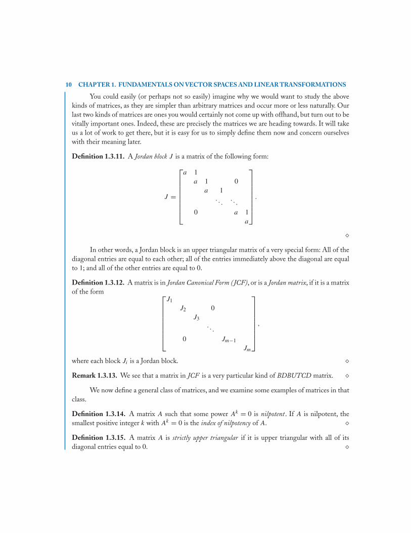
Definition 1.3.11. A Jordan block J is a matrix of the following form:
J =
⎡⎢⎢⎢⎢⎢⎢⎢⎣
a 1a 1 0
a 1. . .
. . .
0 a 1a
⎤⎥⎥⎥⎥⎥⎥⎥⎦
.
�In other words, a Jordan block is an upper triangular matrix of a very special form: All of the
diagonal entries are equal to each other; all of the entries immediately above the diagonal are equalto 1; and all of the other entries are equal to 0.
Definition 1.3.12. A matrix is in Jordan Canonical Form (JCF), or is a Jordan matrix, if it is a matrixof the form ⎡
⎢⎢⎢⎢⎢⎢⎢⎣
J1
J2 0J3
. . .
0 Jm−1
Jm
⎤⎥⎥⎥⎥⎥⎥⎥⎦
,
where each block Ji is a Jordan block. �Remark 1.3.13. We see that a matrix in JCF is a very particular kind of BDBUTCD matrix. �
We now define a general class of matrices, and we examine some examples of matrices in thatclass.
Definition 1.3.14. A matrix A such that some power Ak = 0 is nilpotent . If A is nilpotent, thesmallest positive integer k with Ak = 0 is the index of nilpotency of A. �Definition 1.3.15. A matrix A is strictly upper triangular if it is upper triangular with all of itsdiagonal entries equal to 0. �

1.4. POLYNOMIALS IN T AND A 11
Lemma 1.3.16. Let A be an n-by-n strictly upper triangular matrix. Then A is nilpotent with index ofnilpotency at most n.
Proof. We give two proofs.The first proof is short but not very enlightening.The second proofis longer but more enlightening.
First proof: Direct computation shows that for any strictly upper triangular matrix A, An = 0.(A has all of its diagonal entries 0; A2 has all of its diagonal entries and all of its entries immediatelyabove the diagonal 0; A3 has all of its entries on, one space above, and two spaces above the diagonal0; etc.)
Second proof: Let E = {e1, . . . , en} be the standard basis of Cn and define subspaces V0, . . .,
Vn of Cn as follows: V0 = {0},V1 is the subspace spanned by the vector e1,V2 is the subspace spanned
by the vectors e1 and e2, etc., (so that, in particular, Vn = Cn). If A is strictly upper triangular, then
AVi ⊆ Vi−1 for every i ≥ 1 (and in particular AV1 = {0}). But then A2Vi ⊆ Vi−2 for every i ≥ 2,and A2V2 = A2V1 = {0}. Proceeding in this way we see that AnC
n = AnVn = {0}, i.e.,An = 0.
Lemma 1.3.17. Let J be an n-by-n Jordan block with diagonal entry a. Then J − aI is nilpotent withindex of nilpotency n.
Proof. Again we present two proofs.First proof: A = J − aI is strictly upper triangular, so by Lemma 1.3.16 (J − aI)k = 0 for
some k ≤ n. But direct computation shows that (J − aI)k−1 = 0 (it is the matrix with a 1 in theupper right-hand corner and all other entries 0), so J − aI must have index of nilpotency n.
Second proof: Let A = J − aI . In the notation of the second proof of Lemma 1.3.16, AVi =Vi−1 for every i ≥ 1. Then An−1Vn = V1 = {0}, so An−1 = 0, but AnVn = V0 = {0}, so An = 0,and A has index of nilpotency n.
1.4 POLYNOMIALS IN T AND A
In this section, we consider polynomials in linear transformations T or matrices A. We begin withsome general facts, and then examine some special cases.
All matrices we consider here are square matrices, and all polynomials we consider here havetheir coefficients in the field of complex numbers.
Definition 1.4.1. Let f (x) = anxn + an−1x
n−1 + . . . + a1x + a0 be an arbitrary polynomial.
(1) If T : V −→ V is a linear transformation, we let
f (T ) = anT n + an−1T n−1 + a1T + a0I
where T n denotes the n-fold composition of T with itself (i.e., T 2(v) = T (T (v)),T 3(v) = T (T (T (v))), for every v in V , etc.) and I denotes the identity transformation
12 CHAPTER 1. FUNDAMENTALS ON VECTOR SPACES AND LINEAR TRANSFORMATIONS
(I(v) = v for every v in V ).
(2) If A is a square matrix, we let
f (A) = anAn + an−1A
n−1 + a1A + a0I.
�Lemma 1.4.2. Let T : V −→ V be a linear transformation. Let B be any basis of V , and let A = [T ]B.Then f (A) = [f (T )]B.
Proof. Matrix multiplication is defined as it is precisely by the property that, for any two lineartransformations S and T from V to V , if A = [S]B, and B = [T ]B, then AB = [ST ]B.The lemmaeasily follows from this special case.
Corollary 1.4.3. Let T : V −→ V be a linear transformation. Let B be any basis of V , and let A =[T ]B. Then f (T ) = 0 if and only if f (A) = 0.
Proof. By Lemma 1.4.2, f (A) = [f (T )]B. But a linear transformation is the 0 linear trans-formation if and only if its matrix (in any basis) is the 0 matrix.
Lemma 1.4.4. Let f (x) and g(x) be arbitrary polynomials, and let h(x) = f (x)g(x).
(1) For any linear transformation T , f (T )g(T ) = h(T ) = g(T )f (T ).(2) For any square matrix A, f (A)g(A) = h(A) = g(A)f (A).
Proof. We leave this as an exercise for the reader. (It looks obvious, but there is actuallysomething to prove, and if you try to prove it, you will notice that you use the fact that any twopowers of T , or any two powers of A, commute with each other, something that is not true forarbitrary linear transformations or matrices).
Lemma 1.4.5. Let A and B be similar square matrices, and let P intertwine A and B. Then, for anypolynomial f (x), P intertwines f (A) and f (B). In particular:
(1) f (A) and f (B) are similar; and
(2) f (A) = 0 if and only if f (B) = 0.
Proof. Certainly I = PIP −1. We are given that A = PBP −1. Then A2 =(PBP −1)2 = (PBP −1)(PBP −1) = PB(P −1P)BP −1 = PB2P −1, and then A3 = A2A =(PB2P −1)(PBP −1) = PB2(P −1P)BP −1 = PB3P −1, and similarly Ak = PBkP −1 for everypositive integer k, from which the first part of the lemma easily follows.

1.5. SUBSPACES, COMPLEMENTS, AND INVARIANT SUBSPACES 13
Since we have found a matrix that intertwines f (A) and f (B), they are certainly simi-lar. Furthermore, if f (B) = 0, then f (A) = Pf (B)P −1 = P 0P −1 = 0, while if f (A) = 0, thenf (B) = P −1f (A)P = P −10P = 0.
Lemma 1.4.6. Let f (x) be an arbitrary polynomial.
(1) If A = cI is a scalar matrix, then f (A) is the scalar matrix f (A) = f (c)I .
(2) If A is the diagonal matrix with entries d1, d2, …, dn, then f (A) is the diagonal matrix withentries f (d1), f (d2), …, f (dn).
(3) If A is an upper triangular matrix with entries a1,1, a2,2, …, an,n, then f (A) is an uppertriangular matrix with entries f (a1,1), f (a2,2), …, f (an,n).
Proof. Direct computation.
Lemma 1.4.7. Let f (x) be an arbitrary polynomial.
(1) If A is a block diagonal matrix with diagonal blocks A1, A2, …, Am, then f (A) is the blockdiagonal matrix with entries f (A1), f (A2), …, f (Am).
(3) If A is a block upper triangular matrix with diagonal blocks A1,1, A2,2, …, Am,m, then f (A)
is a block upper triangular matrix with diagonal blocks f (A1,1), f (A2,2), …, f (Am,m).
Proof. Direct computation.
Note that in Lemma 1.4.6 (3) we do not say anything about the off-diagonal entries of f (A),and that in Lemma 1.4.7 (2) we do not say anything about the off-diagonal blocks of f (A).
1.5 SUBSPACES, COMPLEMENTS, ANDINVARIANT SUBSPACES
We begin this section by considering the notion of the complement of a subspace. Afterwards, weintroduce a linear transformation and reconsider the situation.
Definition 1.5.1. Let V be a vector space, and let W1 be a subspace of V . A subspace W2 of V is acomplementary subspace of W1, or simply a complement of W1, if every vector v in V can be writtenuniquely as v = w1 + w2 for some vectors w1 in W1 and w2 in W2. In this situation, V is the directsum of W1 and W2, V = W1 ⊕ W2. �
Note that this definition is symmetric: If W2 is a complement of W1, then W1 is a complementof W2.
Here is a criterion for a pair of subspaces to be mutually complementary.

14 CHAPTER 1. FUNDAMENTALS ON VECTOR SPACES AND LINEAR TRANSFORMATIONS
Lemma 1.5.2. Let W1 and W2 be subspaces of V . Let B1 be any basis of W1 and B2 be any basis of W2.Let B = B1 ∪ B2. Then W1 and W2 are mutually complementary subspaces of V if and only if B is a basisof V .
Proof. Let B1 and B2 be the bases B1 = {v1,1, . . . , v1,i1} and B2 = {v2,1, . . . , v2,i2}. ThenB = {v1,1, . . . , v1,i1, v2,1, . . . , v2,i2}. First suppose that B is a basis of V . Then B spans V , so wemay write any v in V as
v = c1,1v1,1 + . . . + c1,i1v1,i1 + c2,1v2,1 + . . . + c2,i2v2,i2
= (c1,1v1,1 + . . . + c1,i1v1,i1) + (c2,1v2,1 + . . . + c2,i2v2,i2)
= w1 + w2
where w1 = c1,1v1,1 + . . . + c1,i1v1,i1 is in W1 and w2 = c2,1v2,1 + . . . + c2,i2v2,i2 is in W2.Now we must show that this way of writing v is unique. So suppose also v = w′
1 +w′
2 with w′1 = c′
1,1v1,1 + . . . + c′1,i1
v1,i1 and w′2 = c′
2,1v2,1 + . . . + c′2,i2
v2,i2 . Then 0 = v − v =(c1,1 − c′
1,1)v1,1 + . . . + (c1,i1 − c′1,i1
)v1,i1 + (c2,1 − c′2,1)v2,1 + . . . + (c2,i2 − c′
2,i2)v1,i2 . But B is
linearly independent, so we must have c1,1 − c′1,1 = 0, …, c1,i1 − c′
1,i1= 0, …, c2,1 − c′
2,1 = 0,…, c2,i2 − c′
2,i2= 0, i.e., c′
1,1 = c1,1, …, c′1,i1
= c1,i1 , c′2,1 = c2,1, …, c′
2,i2= c2,i2 , so w′
1 = w1 andw′
2 = w2.We leave the proof of the converse as an exercise for the reader.
Corollary 1.5.3. Let W1 be any subspace of V . Then W1 has a complement W2.
Proof. Let B1 = {v1,1, . . . , v1,i1} be any basis of W1. Then B1 is a linearly independentset of vectors in V , so extends to a basis B = {v1,1, . . . , v1,i1, v2,1, . . . , v2,i2} of V . Then B2 ={v2,1, . . . , v2,i2} is a linearly independent set of vectors in V . Let W2 be the subspace of V havingB2 as a basis. Then W2 is a complement of W1.
Remark 1.5.4. If W1 = {0} then W1 has the unique complement W2 = V , and if W1 = V then W1
has the unique complement W2 = {0}. But if W1 is a nonzero proper subspace of V , it never has aunique complement. For there is always more than one way to extend a basis of W1 to a basis of V . �
We will not only want to consider a pair of subspaces, but rather a family of subspaces, andwe can readily generalize Definition 1.5.1 and Lemma 1.5.2.
Definition 1.5.5. Let V be a vector space. A set {W1, . . . , Wk} of subspaces of V is a complementaryset of subspaces of V if every vector v in V can be written uniquely as v = w1 + . . . + wk with wi inWi for each i. In this situation, V is the direct sum of W1, . . ., Wk , V = W1 ⊕ . . . ⊕ Wk .
�Lemma 1.5.6. Let Wi be a subspace of V , for i = 1, . . . , k. Let Bi be any basis of Wi , for each i. LetB = B1 ∪ . . . ∪ Bk . Then {W1, . . . , Wk} is a complementary set of subspaces of V if and only if B is abasis of V .

1.5. SUBSPACES, COMPLEMENTS, AND INVARIANT SUBSPACES 15
Proof. We leave this as an exercise for the reader.
Now we introduce a linear transformation and see what happens.
Definition 1.5.7. Let T : V −→ V be a linear transformation. A subspace W1 of V is invariantunder T , or T -invariant, if T (W1) ⊆ W1, i.e., if T (w1) is in W1 for every vector w1 in W1. �
With the help of matrices, we can easily recognize invariant subspaces.
Lemma 1.5.8. Let T : V −→ V be a linear transformation, where V is an n-dimensional vector space.Let W be an m-dimensional subspace of V and let B1 be any basis of W . Extend B1 to a basis B of V .Then W is a T -invariant subspace of V if and only if
Q = [T ]B =[A B
0 D
]
is a block upper triangular matrix, where A is an m-by-m block.
Proof. Note that the condition for Q to be of this form is simply that the lower left-handcorner of Q is 0.
Let B1 = {v1, . . . , vm} and let B = {v1, . . . , vm, vm+1, . . . , vn}. By Theorem 1.2.4 we knowthat
Q =[q1
∣∣∣∣ q2
∣∣∣∣ . . .
∣∣∣∣ qn
]=
[[T (v1)]B
∣∣∣∣ [T (v2)]B∣∣∣∣ . . .
∣∣∣∣ [T (vn)]B].
First suppose that W is T -invariant. Then for each i between 1 and m, T (vi) is in W , so forsome scalars a1,i , . . ., am,i ,
T (vi) = a1,iv1 + . . . + am,ivm
= a1,iv1 + . . . + am,ivm + 0vm+1 + . . . + 0vn
so
[T (vi)]B =
⎡⎢⎢⎢⎢⎢⎢⎢⎢⎣
a1,i
...
am,i
0...
0
⎤⎥⎥⎥⎥⎥⎥⎥⎥⎦
and Q is block upper triangular as claimed.Conversely, suppose that Q is block upper triangular as above. Let v = vi for i between 1 and
m. Then, if A has entries {ai,j }, then, again by Theorem 1.2.4,
T (vi) = a1,iv1 + . . . + am,ivm + 0vm+1 + . . . + 0vn
= a1,iv1 + . . . + am,ivm
16 CHAPTER 1. FUNDAMENTALS ON VECTOR SPACES AND LINEAR TRANSFORMATIONS
and so T (vi) is in W . Since this is true for every element of the basis B1 of W , it is true for everyelement of W , and so T (W) ⊆ W , and W is T -invariant.
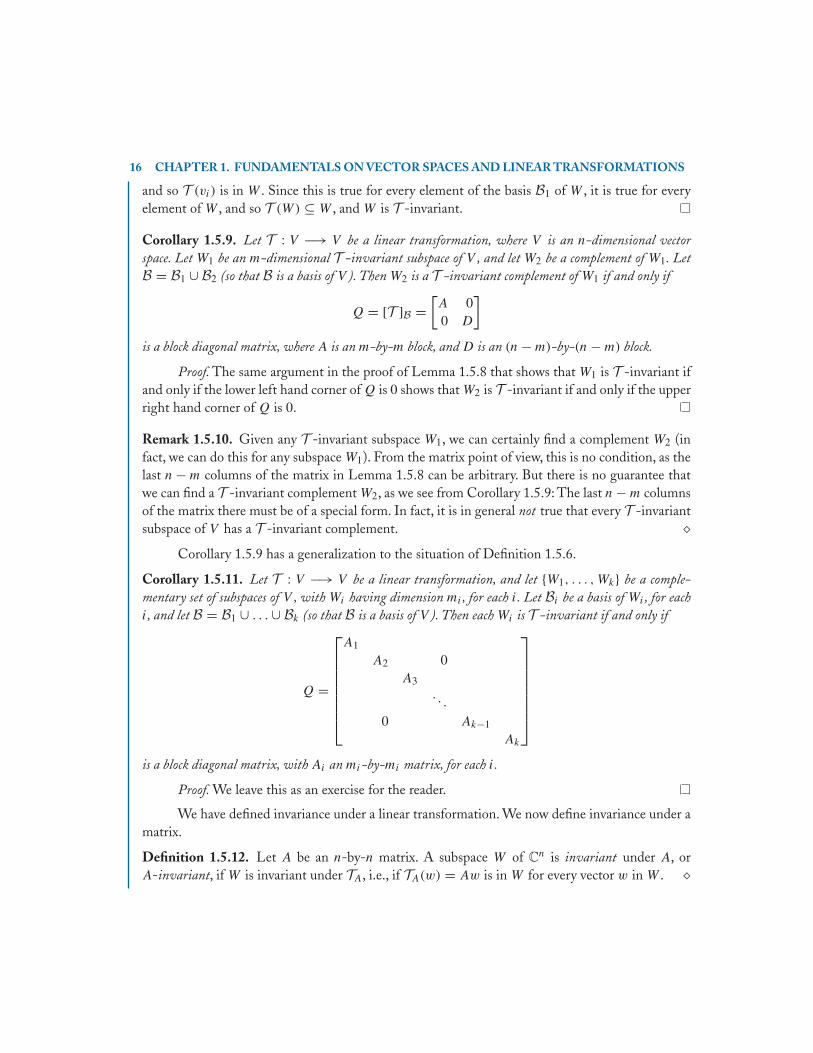
Corollary 1.5.9. Let T : V −→ V be a linear transformation, where V is an n-dimensional vectorspace. Let W1 be an m-dimensional T -invariant subspace of V , and let W2 be a complement of W1. LetB = B1 ∪ B2 (so that B is a basis of V ). Then W2 is a T -invariant complement of W1 if and only if
Q = [T ]B =[A 00 D
]
is a block diagonal matrix, where A is an m-by-m block, and D is an (n − m)-by-(n − m) block.
Proof. The same argument in the proof of Lemma 1.5.8 that shows that W1 is T -invariant ifand only if the lower left hand corner of Q is 0 shows that W2 is T -invariant if and only if the upperright hand corner of Q is 0.
Remark 1.5.10. Given any T -invariant subspace W1, we can certainly find a complement W2 (infact, we can do this for any subspace W1). From the matrix point of view, this is no condition, as thelast n − m columns of the matrix in Lemma 1.5.8 can be arbitrary. But there is no guarantee thatwe can find a T -invariant complement W2, as we see from Corollary 1.5.9: The last n − m columnsof the matrix there must be of a special form. In fact, it is in general not true that every T -invariantsubspace of V has a T -invariant complement. �
Corollary 1.5.9 has a generalization to the situation of Definition 1.5.6.
Corollary 1.5.11. Let T : V −→ V be a linear transformation, and let {W1, . . . , Wk} be a comple-mentary set of subspaces of V , with Wi having dimension mi , for each i. Let Bi be a basis of Wi , for eachi, and let B = B1 ∪ . . . ∪ Bk (so that B is a basis of V ). Then each Wi is T -invariant if and only if
Q =
⎡⎢⎢⎢⎢⎢⎢⎢⎣
A1
A2 0A3
. . .
0 Ak−1
Ak
⎤⎥⎥⎥⎥⎥⎥⎥⎦
is a block diagonal matrix, with Ai an mi-by-mi matrix, for each i.
Proof. We leave this as an exercise for the reader.
We have defined invariance under a linear transformation. We now define invariance under amatrix.
Definition 1.5.12. Let A be an n-by-n matrix. A subspace W of Cn is invariant under A, or
A-invariant, if W is invariant under TA, i.e., if TA(w) = Aw is in W for every vector w in W . �

17
C H A P T E R 2
The Structure of a LinearTransformation
Let V be a vector space and let T : V −→ V be a linear transformation. Our objective in thischapter is to prove that V has a basis B in which [T ]B is a matrix in Jordan Canonical Form. Statedin terms of matrices, our objective is to prove that any square matrix A is similar to a matrix J inJordan Canonical Form. (Throughout this chapter, we will feel free to switch between the languageof matrices and the language of linear transformations. It is some times more convenient to use theone, and sometimes more convenient to use the other.)
Before we do this, we must introduce some basic structural notions: eigenvalues, eigenvectors,generalized eigenvectors, and the characteristic and minimum polynomials of a matrix or of a lineartransformation.
2.1 EIGENVALUES, EIGENVECTORS, ANDGENERALIZED EIGENVECTORS
In this section, we introduce eigenvalues, eigenvectors, and generalized eigenvectors, as well as thecharacteristic polynomial. First, we begin by considering matrices, and then we consider lineartransformations.
Definition 2.1.1. Let A be an n-by-n matrix. If v = 0 is a vector such that, for some λ,
Av = λv
then v is an eigenvector of A associated to the eigenvalue λ. �Remark 2.1.2. We note that the definition of an eigenvalue/eigenvector can be expressed in analternate form.
Av = λv
Av = λIv
(A − λI)v = 0.
�Definition 2.1.3. For an eigenvalue a of A, we let E(λ) denote the eigenspace of λ,
E(λ) = {v | Av = λv} = {v | (A − λI)v = 0} = Ker(A − λI).
�

18 CHAPTER 2. THE STRUCTURE OF A LINEAR TRANSFORMATION
We also note that the formulation in Remark 2.1.2 helps us find eigenvalues and eigenvectors.For if (A − λI)v = 0 for a nonzero vector v, the matrix A − λI must be singular, and hence itsdeterminant must be 0. This leads us to the following definition.
Definition 2.1.4. The characteristic polynomial of a matrixA is the polynomial cA(x) = det(xI − A).�
Remark 2.1.5. This is the customary definition of the characteristic polynomial. But note that, if A
is an n-by-n matrix, then the matrix xI − A is obtained from the matrix A − xI by multiplying eachof its n rows by −1, and hence det(xI − A) = (−1)n det(A − xI). In practice, it is most convenientto work with A − xI in finding eigenvectors, as this minimizes arithmetic. Furthermore, when wecome to finding chains of generalized eigenvectors, it is (almost) essential to use A − xI , as usingxI − A would introduce lots of spurious minus signs. �Remark 2.1.6. Since A is an n-by-n matrix, we see from properties of the determinant that cA(x) =det(xI − A) is a polynomial of degree n. �
We have the following important and useful fact about characteristic polynomials.
Lemma 2.1.7. Let A and B be similar matrices. Then they have the same characteristic polynomial, i.e.,cA(x) = cB(x).
Proof. Let A = PBP −1. Then xI − A = xI − PBP −1 = x(P IP −1) − PBP −1 =P(xI)P −1 − PBP−1 = P(xI − B)P −1, so cA(x) = det(xI − A) = det(P (xI − B)P −1) =det(P ) det(xI − B) det(P −1) = det(xI − B) = cB(x).
The practical use of Lemma 2.1.7 is that, if we wish to compute the characteristic polynomialcA(x) of the matrix A, we may instead “replace” A by a similar matrix B, whose characteristicpolynomial cB(x) is easier to compute, and compute that. There is also an important theoretical useof this lemma, as we will see in Definition 2.1.23 below.
Here are some cases in which the characteristic polynomial is (relatively) easy to compute.These cases are important both in theory and in practice.
Lemma 2.1.8. Let A be the diagonal matrix with diagonal entries d1, . . ., dn. Then cA(x) = (x −d1) · · · (x − dn).
More generally, let A be an upper triangular matrix with diagonal entries a1,1, . . ., an,n. ThencA(x) = (x − a1,1) · · · (x − an,n).
Proof. If A is the diagonal matrix with diagonal entries d1, . . ., dn, then xI − A is the diagonalmatrix with diagonal entries x − d1, . . ., x − dn. But the determinant of a diagonal matrix is theproduct of its diagonal entries. More generally, if A is an upper triangular matrix with diagonalentries a1,1, . . ., an,n, then xI − A is an upper triangular matrix with diagonal entries x − a1,1,. . ., x − an,n. But the determinant of an upper triangular matrix is also the product of its diagonalentries.
2.1. EIGENVALUES, EIGENVECTORS, AND GENERALIZED EIGENVECTORS 19
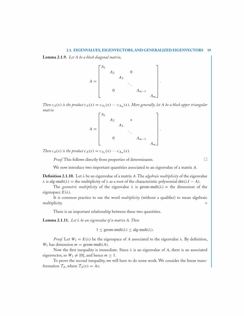
Lemma 2.1.9. Let A be a block diagonal matrix,
A =
⎡⎢⎢⎢⎢⎢⎢⎢⎣
A1
A2 0A3
. . .
0 Am−1
Am
⎤⎥⎥⎥⎥⎥⎥⎥⎦
.
Then cA(x) is the product cA(x) = cA1(x) · · · cAm(x). More generally, let A be a block upper triangularmatrix
A =
⎡⎢⎢⎢⎢⎢⎢⎢⎣
A1
A2 ∗A3
. . .
0 Am−1
Am
⎤⎥⎥⎥⎥⎥⎥⎥⎦
.
Then cA(x) is the product cA(x) = cA1(x) · · · cAm(x).
Proof. This follows directly from properties of determinants.
We now introduce two important quantities associated to an eigenvalue of a matrix A.
Definition 2.1.10. Let λ be an eigenvalue of a matrix A. The algebraic multiplicity of the eigenvalueλ is alg-mult(λ) = the multiplicity of λ as a root of the characteristic polynomial det(λI − A).
The geometric multiplicity of the eigenvalue λ is geom-mult(λ) = the dimension of theeigenspace E(λ).
It is common practice to use the word multiplicity (without a qualifier) to mean algebraicmultiplicity. �
There is an important relationship between these two quantities.
Lemma 2.1.11. Let λ be an eigenvalue of a matrix A. Then
1 ≤ geom-mult(λ) ≤ alg-mult(λ).
Proof. Let W1 = E(λ) be the eigenspace of A associated to the eigenvalue λ. By definition,W1 has dimension m = geom-mult(A).
Now the first inequality is immediate. Since λ is an eigenvalue of A, there is an associatedeigenvector, so W1 = {0}, and hence m ≥ 1.
To prove the second inequality, we will have to do some work. We consider the linear trans-formation TA, where TA(v) = Av.
20 CHAPTER 2. THE STRUCTURE OF A LINEAR TRANSFORMATION
By definition, W1 has dimension m = geom-mult(λ). Then W1 is a TA-invariant subspace ofC
n, as for any vector v in W1, TA(v) = Av = λv is in W1. Let W2 be any complement of W1 in Cn.
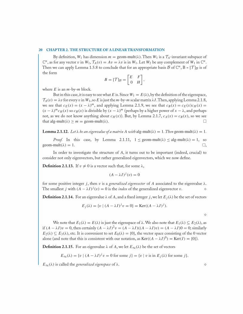
Then we can apply Lemma 1.5.8 to conclude that for an appropriate basis B of Cn, B = [T ]B is of
the form
B = [T ]B =[E F
0 H
],
where E is an m-by-m block.But in this case, it is easy to see what E is.Since W1 = E(λ), by the definition of the eigenspace,
TA(v) = λv for every v in W1, so E is just the m-by-m scalar matrix λI .Then, applying Lemma 2.1.8,we see that cE(x) = (x − λ)m, and applying Lemma 2.1.9, we see that cB(x) = cE(x)cH (x) =(x − λ)mcH (x) so cB(x) is divisible by (x − λ)m (perhaps by a higher power of x − λ, and perhapsnot, as we do not know anything about cH (x)). But, by Lemma 2.1.7, cA(x) = cB(x), so we seethat alg-mult(λ) ≥ m = geom-mult(λ).
Lemma 2.1.12. Let λ be an eigenvalue of a matrix A with alg-mult(λ) = 1. Then geom-mult(λ) = 1.
Proof. In this case, by Lemma 2.1.11, 1 ≤ geom-mult(λ) ≤ alg-mult(λ) = 1, sogeom-mult(λ) = 1. ,
In order to investigate the structure of A, it turns out to be important (indeed, crucial) toconsider not only eigenvectors, but rather generalized eigenvectors, which we now define.
Definition 2.1.13. If v = 0 is a vector such that, for some λ,
(A − λI)j (v) = 0
for some positive integer j , then v is a generalized eigenvector of A associated to the eigenvalue λ.The smallest j with (A − λI)j (v) = 0 is the index of the generalized eigenvector v. �Definition 2.1.14. For an eigenvalue λ of A, and a fixed integer j , we let Ej(λ) be the set of vectors
Ej(λ) = {v | (A − λI)j v = 0} = Ker((A − λI)j ).
�We note that E1(λ) = E(λ) is just the eigenspace of λ. We also note that E1(λ) ⊆ E2(λ), as
if (A − λI)v = 0, then certainly (A − λI)2v = (A − λI)((A − λI)v) = (A − λI)0 = 0; similarlyE2(λ) ⊆ E3(λ), etc. It is convenient to set E0(λ) = {0}, the vector space consisting of the 0 vectoralone (and note that this is consistent with our notation, as Ker((A − λI)0) = Ker(I ) = {0}).Definition 2.1.15. For an eigenvalue λ of A, we let E∞(λ) be the set of vectors
E∞(λ) = {v | (A − λI)j v = 0 for some j} = {v | v is in Ej(λ) for some j}.E∞(λ) is called the generalized eigenspace of λ. �

2.1. EIGENVALUES, EIGENVECTORS, AND GENERALIZED EIGENVECTORS 21
Lemma 2.1.16. Let λ be an eigenvector of A. For any j , Ej(λ) is a subspace of Cn. Also, E∞(λ) is a
subspace of Cn.
Proof. Ej(λ) is the kernel of the linear transformation T(A−λI)j , and the kernel of a lineartransformation is always a subspace. We leave the proof for E∞(λ) to the reader.
In fact, these are not only subspaces but in fact A-invariant subspaces. Indeed, this is one ofthe most important ways in which invariant subspaces arise.
Lemma 2.1.17. Let A be an n-by-n matrix and let λ be an eigenvalue of A. Then for any j , Ej(λ) isan A-invariant subspace of C
n. Also, E∞(λ) is an A-invariant subspace of Cn.
Proof. Let v be any vector in Ej(λ), and let w = Av. By definition, (A −λI)j v = 0. But then (A − λI)jw = (A − λI)j (Av) = ((A − λI)jA)v = (A(A − λI)j )v =A((A − λI)j v) = A0 = 0, so Aw is in Ej(λ). Since any vector in E∞(λ) is in Ej(λ) for somej , this also shows that E∞(λ) is A-invariant.
Here is a very useful computational lemma.
Lemma 2.1.18. Let A be an n-by-n matrix and let λ be an eigenvalue of A. Let f (x) be any polynomial.If v is any eigenvector of A associated to the eigenvalue λ, then f (A)v = f (λ)v. More generally, if v
is any generalized eigenvector of A of index j associated to the eigenvalue λ, then f (A)v = f (λ)v + v′where v′ is in Ej−1(λ).
Proof. By definition, Av = λv. Then A2v = A(Av) = A(λv) = λ(Av) = λ2v, and similarlyAiv = λiv for any positive integer i, from which the first claim follows.
Now for the second claim. By the division algorithm for polynomials, we can writef (x) as f (x) = (x − λ)q(x) + f (λ) for some polynomial q(x) (i.e., f (λ) is the remainderupon dividing f (x) by x − λ). Then f (A) = (A − λI)q(A) + f (λ)I . Now let v be a general-ized eigenvector of A of index j associated to λ. Then f (A)v = (A − λI)q(A)v + f (λ)Iv =v′ + f (λ)v. Furthermore, (A − λI)j−1v′ = (A − λI)j−1((A − λI)q(A))v = ((A − λI)j−1(A −λI)q(A))v = ((A − λI)jq(A))v = (q(A)(A − λI)j )v = q(A)((A − λI)j v) = q(A)0 = 0, so v′is in Ej−1(λ).
From its definition, it appears that we may have to consider arbitrarily high powers of j infinding E∞(λ). But in fact we do not, as we see from the next proposition.
Proposition 2.1.19. Let A be an square matrix and let λ be an eigenvalue of A. Let E∞(λ) be a subspaceof C
n of dimension d∞(λ). Then E∞(λ) = Ej(λ) for some j ≤ d∞(λ). Furthermore, the smallest valueof j for which E∞(λ) = Ej(λ) is equal to the smallest value of j for which Ej+1(λ) = Ej(λ).
Proof. First note that since E∞(λ) is a subspace of Cn, d∞(λ) ≤ n.
Let di(λ) = dim Ei(λ) for each positive integer i. Since Ei(λ) ⊆ Ei+1(λ), we have thatdi(λ) ≤ di+1(λ). Furthermore, d1(λ) ≥ 1, as, by definition, E1(λ) is a nonzero vector space (thereis some eigenvector in it), and di(λ) ≤ d∞(λ) for every i, as each Ei(λ) is a subspace of E∞(λ).

22 CHAPTER 2. THE STRUCTURE OF A LINEAR TRANSFORMATION
Thus we have a sequence of positive integers 1 ≤ d1(λ) ≤ d2(λ) < . . . < d∞(λ), all of which areless than or equal to n, so this sequence cannot continually strictly increase, i.e., there is a value ofj for which dj (λ) = dj+1(λ). Furthermore, this must occur for j ≤ d∞(λ), as the longest possiblystrictly increasing sequence of integers between 1 and d∞(λ) is 1 < 2 < . . . < d∞(λ), a sequenceof length d∞(λ).
We claim that Ej(λ) = Ej+1(λ) = Ej+2(λ) = . . ., so (dj (λ) = dj+1(λ) = dj+2(λ) = . . .)and E∞(λ) = Ej(λ). To see this claim, first observe that Ej(λ) ⊆ Ej+1(λ) and dim Ek(λ) =dim Ej+1(λ), so Ej(λ) = Ej+1(λ).
Now Ej+2(λ) = {v | (A − λI)j+2v = 0} = {v | (A − λI)j+1((A − λI)v) = 0}. But theequality Ej(λ) = Ej+1(λ) tells us that for any vector w, (A − λI)j+1w = 0 if and only if(A − λI)jw = 0; in particular, this is true for w = (A − λI)v. Applying this, we see that Ej+2(λ) ={v | (A − λI)j ((A − λI)v) = 0} = {v | (A − λI)j+1v = 0} = Ej+1(λ), etc.
With this proposition in hand, we can introduce a third important quantity associated to aneigenvalue a of A.
Definition 2.1.20. Let λ be an eigenvalue of a matrix A. Then max-ind(λ) , the maximum index ofa generalized eigenvector of A associated to λ, is the largest value of j such that A has a generalizedeigenvector of index j associated to the eigenvalue λ. Equivalently, max-ind(λ) is the smallest valueof j such that Ej(λ) = E∞(λ). �Corollary 2.1.21. Let A be an square matrix and let λ be an eigenvalue of A. Then max-ind(λ) is lessthan or equal to the dimension of E∞(λ).
Proof. This is just a restatement of Proposition 2.1.19 using the language of Definition 2.1.20.
Remark 2.1.22. It appears that we have a fourth important quantity associated to an eigenvalue λ
of A, namely d∞(λ). But we shall see below that d∞(λ) = alg-mult(λ). We shall also see that theindividual numbers d1(λ), d2(λ), . . . play an important role. �
Now we wish to consider an arbitrary linear transformation T : V −→ V instead ofjust a square matrix A. We observe that almost everything we have done is exactly the same.For example, we can define the eigenspace E(λ) of T by E(λ) = Ker(T − λI), the spacesEj(λ) by Ej(λ) = Ker((T − λI)j ), and similarly the generalized eigenspace E∞(λ) by E∞(λ) ={v | v is in Ej(λ) for some j}. The one potential difficulty is in defining the characteristic polyno-mial, as it is not a priori clear what we mean by det(xI − T ). It is given as follows.
Definition 2.1.23. Let T : V −→ V be a linear transformation. Let B be a basis of V and setA = [T ]B. Then the characteristic polynomial of T is cT (x) = cA(x) = det(xI − A). �
Note that this definition makes sense. We have to choose a basis B to get the matrix A. If wechoose another basis C, we get another matrix B. But, by Theorem 1.2.8, A and B are similar, and

2.2. THE MINIMUM POLYNOMIAL 23
then by Lemma 2.1.7, cA(x) = cB(x). Thus it doesn’t matter which basis we choose. In fact, we willbe using this observation not only to know that the characteristic polynomial of T is well-defined,but also to be able to switch bases to find a basis in which it is easiest to compute. (Actually, wealready have used it for this purpose in the proof of Lemma 2.1.11.)
Remark 2.1.24. Note that, following our previous notation, if T = TA is the linear transformationgiven by TA(v) = Av, then cT (x) = cTA
(x) = cA(x). �
2.2 THE MINIMUM POLYNOMIALIn the previous section, we introduced an extremely important polynomial associated to a lineartransformation or to a matrix: its characteristic polynomial. In this section, we introduce a secondextremely important polynomial associated to a linear transformation or to a matrix: its minimumpolynomial.
Proposition 2.2.1. (1) Let A be an n-by-n matrix. Then there is a unique monic polynomial mA(x) ofsmallest degree with mA(A) = 0.
Proof. We begin by showing that there is some nonzero polynomial f (x) with f (A) = 0.Step 0: Note that the set {I } consisting of the identity matrix alone is linearly independent.Step 1: Consider the set of matrices {I, A}. If this set is linearly dependent, then we have a
relation c0I + c1A = 0 with c1 = 0, and so, setting f (x) = c0 + c1x, then f (A) = 0.Step 2: If {I, A} is linearly independent, consider the set of matrices {I, A, A2}. If this set
is linearly dependent, then we have a relation c0I + c1A + c2A2 = 0 with c2 = 0, and so, setting
f (x) = c0 + c1x + c2x2, then f (A) = 0.
Keep going. If this procedure stops at some step, then we have found such a polynomial f (x).But this procedure must stop no later than step n2, as at that step we have the set {I, A, . . . , An2}, aset of n2 + 1 elements of the vector space of n-by-n matrices. But this vector space has dimensionn2, so this set must be linearly dependent.
We want a monic polynomial, but this is easy to arrange: If f (x) = ckxk + ck−1x
k−1 =. . . + c0, let mA(x) = (1/ck)f (x) = xk + ak−1x
k−1 + . . . + a0 where ai = ci/ck−1..Finally, we want to show this polynomial is unique. So suppose we had another monic
polynomial g(x) = xk + bk−1xk−1 + . . . + b0 with g(A) = 0. Let h(x) = mA(x) − g(x). Then
h(A) = mA(A) − g(A) = 0 − 0 = 0. But h(x) has degree less than k (as the xk terms cancel).However, k is the smallest degree of a nonzero polynomial f (x) with f (A) = 0, so h(x) must bethe zero polynomial and hence g(x) = mA(x).
This proposition leads us to a definition.
Definition 2.2.2. Let A be a matrix.The minimum polynomial of A is the unique monic polynomialmA(x) of smallest degree with mA(A) = 0. �Lemma 2.2.3. Let A and B be similar matrices. Then mA(x) = mB(x).
24 CHAPTER 2. THE STRUCTURE OF A LINEAR TRANSFORMATION
Proof. Immediate from Lemma 1.4.5.
Remark 2.2.4. Let us emphasize the conclusion of Lemma 2.2.3. If we wish to find mA(x), we mayreplace A by a similar but hopefully simpler matrix B and instead find mB(x). �Corollary 2.2.5. Let A be an n-by-n matrix. Then mA(x) is a polynomial of degree at most n2.
Proof. Immediate from the proof of Proposition 2.2.1.
Remark 2.2.6. We shall be investigating the minimum polynomial a lot more deeply, and we shallsee that in fact the minimum polynomial of an n-by-n matrix has degree at most n. �
The following proposition plays an important role.
Proposition 2.2.7. Let A be an n-by-n matrix and let f (x) be any polynomial with f (A) = 0. Thenf (x) is divisible by mA(x).
Proof. Let mA(x) be a polynomial of degree k. By the division algorithm for polynomials,we may write f (x) = mA(x)q(x) + r(x) where either r(x) = 0 is the zero polynomial, or r(x)
is a nonzero polynomial of degree less than k. But then r(x) = f (x) − mA(x)q(x) so r(A) =f (A) − mA(A)q(A) = 0 − 0q(A) = 0 − 0 = 0. If r(x) were a nonzero polynomial, it would bea nonzero polynomial of degree less than k with r(A) = 0. By the definition of the minimumpolynomial, no such polynomial can exist. Hence we must have r(x) = 0, so f (x) = mA(x)q(x) isa multiple of mA(x).
Now let us examine some examples of matrices, with a view towards determining their char-acteristic and minimum polynomials.
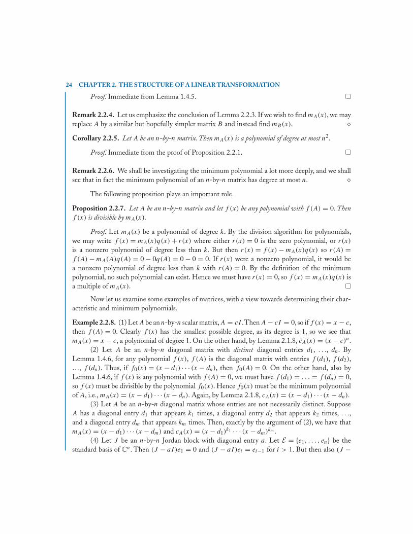
Example 2.2.8. (1) Let A be an n-by-n scalar matrix,A = cI .Then A − cI = 0, so if f (x) = x − c,then f (A) = 0. Clearly f (x) has the smallest possible degree, as its degree is 1, so we see thatmA(x) = x − c, a polynomial of degree 1. On the other hand, by Lemma 2.1.8, cA(x) = (x − c)n.
(2) Let A be an n-by-n diagonal matrix with distinct diagonal entries d1, . . ., dn. ByLemma 1.4.6, for any polynomial f (x), f (A) is the diagonal matrix with entries f (d1), f (d2),…, f (dn). Thus, if f0(x) = (x − d1) · · · (x − dn), then f0(A) = 0. On the other hand, also byLemma 1.4.6, if f (x) is any polynomial with f (A) = 0, we must have f (d1) = . . . = f (dn) = 0,so f (x) must be divisible by the polynomial f0(x). Hence f0(x) must be the minimum polynomialof A, i.e., mA(x) = (x − d1) · · · (x − dn). Again, by Lemma 2.1.8, cA(x) = (x − d1) · · · (x − dn).
(3) Let A be an n-by-n diagonal matrix whose entries are not necessarily distinct. SupposeA has a diagonal entry d1 that appears k1 times, a diagonal entry d2 that appears k2 times, . . .,and a diagonal entry dm that appears km times. Then, exactly by the argument of (2), we have thatmA(x) = (x − d1) · · · (x − dm) and cA(x) = (x − d1)
k1 · · · (x − dm)km .(4) Let J be an n-by-n Jordan block with diagonal entry a. Let E = {e1, . . . , en} be the
standard basis of Cn. Then (J − aI)e1 = 0 and (J − aI)ei = ei−1 for i > 1. But then also (J −

2.2. THE MINIMUM POLYNOMIAL 25
aI)2ei = 0 for i = 1, 2 and (J − aI)2ei = 0 for i > 2. Proceeding in this way, we find that (J −aI)n−1en = e1, so (J − aI)n−1 = 0, but that (J − aI)nei = 0 for every i, which implies that (J −aI)n = 0 (as E is a basis of C
n). Thus we see that if f0(x) = (x − a)n, then f0(J ) = 0. Hence, byProposition 2.2.6, mJ (x) must divide (x − a)n, so we must have mJ (x) = (x − a)k for some k ≤ n.But we just observed that if f (x) = (x − a)n−1, then f (J ) = 0. Hence we must have k = n. Thuswe see that mJ (x) = (x − a)n. Also, cJ (x) = (x − a)n. (Note that the first part of this argument isessentially the argument of the proof of Lemma 1.3.17.)
(6) Let A be an n-by-n upper triangular matrix with distinct diagonal entries d1, . . ., dn. ByLemma 1.4.6, for any polynomial f (x),f (A) is an upper triangular matrix with entries f (d1),f (d2),…, f (dn).Thus, if f (x) is any polynomial with f (A) = 0, we must have f (d1) = . . . = f (dn) = 0,so f (x) must be divisible by the polynomial f0(x) = (x − d1) · · · (x − dn).On the other hand, a veryunenlightening computation shows that f0(x) = 0. Hence f0(x) must be the minimum polynomialof A, i.e., mA(x) = (x − d1) · · · (x − dn). Also, cA(x) = (x − d1) · · · (x − dn).
(7) Let A be an n-by-n upper triangular matrix with diagonal entries d1 appearing k1 times,d2 appearing k2 times, . . ., and dm appearing km times. The argument of (6) shows that if f (x)
is any polynomial with f (A) = 0, then f (x) must be divisible by f0(x) = (x − d1) · · · (x − dm).On the other hand, if f1(x) = (x − d1)
k1 · · · (x − dm)km , then a very unenlightening computationshows that f1(A) = 0. Hence f0(x) divides mA(x), which divides f1(x).Thus we see that mA(x) =(x − d1)
j1 · · · (x − dm)jm for some integers 1 ≤ j1 ≤ k1, . . ., 1 ≤ jm ≤ km. Without any furtherinformation about A, we cannot specify the integers {ji} more precisely. But in any case, cA(x) =(x − d1)
k1 · · · (x − dm)km . �
Remark 2.2.9. The easiest way to do the computations in Example 2.2.8 (6) and (7) is to use thefollowing computational result, whose proof we leave to you: Let M1, . . ., Mn be n n-by-n uppertriangular matrices and suppose that, for each i between 1 and n, the ith diagonal entry of Mi is 0.Then M1 · · · Mn = 0. But no matter how you do it, this is a computation that does not yield muchinsight. We will see below why these results are true. �
For a polynomial f (x) = (x − a1)k1 · · · (x − am)km , we call the factors x − ai the irreducible
factors of f (x).We record here the two basic facts relating mA(x) and cA(x). For any square matrix A:
(1) mA(x) and cA(x) have the same irreducible factors; and
(2) mA(x) divides cA(x).
You can see that these are both true in all parts of Example 2.2.8. We will prove the first ofthese now, but we will have to do more work before we can prove the second.
Theorem 2.2.10. Let A be any square matrix.Then its minimum polynomial mA(x) and its characteristicpolynomial cA(x) have the same irreducible factors.

26 CHAPTER 2. THE STRUCTURE OF A LINEAR TRANSFORMATION
Proof. First, we show that every irreducible factor of cA(x) is an irreducible factor of mA(x):Let x − a be an irreducible factor of cA(x). Then a is an eigenvalue of A. Choose any associatedeigenvector v. Since mA(A) = 0, certainly mA(A)v = 0. But by Lemma 2.1.18,mA(A)v = mA(a)v.Thus 0 = mA(a)v. Since v = 0, we must have mA(a) = 0, and so x − a divides mA(x).
Next, we show that every irreducible factor of mA(x) is an irreducible factor of cA(x): Letx − a be an irreducible factor of mA(x). Write mA(x) = (x − a)q(x). Now q(A) = 0, as q(x)
is a polynomial of smaller degree that of mA(x). Thus w = q(A)v = 0 for some vector w. Butthen (A − aI)w = (A − aI)(q(A)v) = ((A − aI)q(A))v = mA(A)v = 0. In other words, w is aneigenvector of A with associated eigenvalue a, and so x − a divides cA(x).
Again, we may rephrase this in terms of linear transformations.
Definition 2.2.11. Let T : V −→ V be a linear transformation. The minimum polynomial of T isthe unique monic polynomial mT (x) of smallest degree with mT (T ) = 0. �
Again, we should note that this definition makes sense. In this situation, let B be any basisof V and let A = [T ]B. Then A has a minimum polynomial, and mT (x) = mA(x). Furthermore,this is well-defined, as if C is any other basis of V , and B = [T ]C , then A and B are similar, somA(x) = mB(x). Thus we see that mT (x) is independent of the choice of basis.
Remark 2.2.12. Note that, following our previous notation, if T = TA is the linear transformationgiven by TA(v) = Av, then mT (x) = mTA
(x) = mA(x). �
2.3 REDUCTION TO BDBUTCD FORM
Having begun by introducing some basic structural features of a linear transformation (or matrix),we now embark on our derivation of Jordan Canonical Form. This is a very long argument, and sowe carry it out in steps. The first step, which we carry out in this section, is to show that we can getA to be in BDBUTCD form. Recall from Definition 1.3.8 that a matrix in BDBUTCD form is ablock diagonal matrix whose blocks are upper triangular with constant diagonal.
We state this as a theorem.
Theorem 2.3.1. Let V be a vector space and let T : V −→ V be a linear transformation. Then V has abasis B in which A = [T ]B is a matrix in BDBUTCD form.
Proof. Let V have dimension n. We prove this by induction on n.
If n = 1, then the only possible linear transformation T is T (v) = λv for some λ, and then,in any basis B, [T ]B is the 1-by-1 matrix [λ], which is certainly in BDBUTCD form.
Now for the inductive step. In the course of this argument, we will sometimes be explicitlychanging bases, and sometimes conjugating by nonsingular matrices. Of course, these have the sameeffect (cf. Remark 1.2.12), but sometimes one will be more convenient than the other.

2.3. REDUCTION TO BDBUTCD FORM 27
Let cT (x) = (x − λ1)k1(x − λ2)
k2 · · · (x − λm)km . Let v1 be an eigenvector of T with as-sociated eigenvalue λ1. Let W1 be the subspace of V spanned by v1. Since v1 is an eigenvector ofT , W1 is a T -invariant subspace of V , by Lemma 2.1.16. Extend {v1} to a basis D of V . Then, byLemma 1.5.8, we have that [T ]D is a block upper triangular matrix,
Q = [T ]D =[λ1 B
0 D
],
where B is a 1-by-(n − 1) matrix and D is an (n − 1)-by-(n − 1) matrix. By Lemma 2.1.9, cQ(x) =(x − λ1)cD(x), so cD(x) = (x − λ1)
k1−1(x − λ2)k2 · · · (x − λm)km . We now apply the inductive
hypothesis to conclude that there is an (n − 1)-by-(n − 1) matrix P0 such that H = PDP −1 is inBDBUTCD form, and indeed with its first k1 − 1 diagonal entries equal to λ1. Let P be the n-by-nblock diagonal matrix
P =[
1 00 P0
].
Then direct computation shows that
R = PQP −1 =[λ1 F
0 H
],
a block upper triangular matrix whose first k1 diagonal entries are equal to λ1. This is good, but notgood enough. We need to “improve” R so that it is in BDBUTCD form.
Let F = [r1,2 . . . r1,n
]. The first k1 − 1 entries of F are no problem. Since the first k1 − 1
diagonal entries of H are equal to λ1, we can “absorb” the upper left hand corner of R into a singlek1-by-k1 block.
The remaining entries of F do present a problem. For simplicity of notation as we solve thisproblem, let us simply set k = k1.
Now R = [T ]C in some basis C of V . Let C = {w1, . . . , wn}. We will replace each wt , fort > k, with a new vector us so as to eliminate the problematic entries of F . We do this one vector ata time, beginning with t = k + 1. To this end, let ut = wt + ctw1 where ct is a constant yet to bedetermined. If R has entries {ri,j }, then
T (wt ) = r1,tw1 + r2,tw2 + . . . rk,twk + rt,twt ,
andT (ctw1) = ctλ1w1,
so
T (ut ) = T (wt + ctw1) = (r1,t + ctλ1)w1 + r2,tw2 + . . . rk,twk + rt,twt
= (r1,t + ctλ1)w1 + r2,tw2 + . . . rk,twk + rt,t (ut − ctw1)
= (r1,t + ctλ1 − ct rt,t )w1 + r2,tw2 + . . . rk,twk + rt,tut .

28 CHAPTER 2. THE STRUCTURE OF A LINEAR TRANSFORMATION
The coefficient of w1 in this expression is r1,t + ctλ1 − ct rt,t = r1,t + ct (λ1 − rt,t ). Note that λ1 −rt,t = 0, as the first k = k1 diagonal entries of R are equal to λ1, but the remaining diagonal entriesof R are unequal to λ1. Hence if we choose
ct = −r1,t /(λ1 − rt,t )
we see that the w1-coefficient of T (ut ) is equal to 0. In other words, the matrix of T in the basis{w1, . . . , wk, uk+1, wk+2, . . . , wn} is of the same form as R, except that the entry in the (1, k + 1)
position is 0. Now do the same thing successively for t = k + 2, . . ., n. When we have finished weobtain a basis B = {w1, . . . , wk, uk+1, . . . , un} with A = [T ]B of the form
A = [T ]B =[M 00 N
]
with M and N each in BDBUTCD form, in which case A itself is in BDBUTCD form, as required.
Actually, we proved a more precise result than we stated. Let us state that more precise resultnow.
Theorem 2.3.2. Let V be a vector space and let T : V −→ V be a linear transformation with char-acteristic polynomial cT (x) = (x − λ1)
k1(x − λ2)k2 · · · (x − λm)km . Then V has a basis B in which
A = [T ]B is a block diagonal matrix
A =
⎡⎢⎢⎢⎢⎢⎢⎢⎣
A1
A2 0A3
. . .
0 Am−1
Am
⎤⎥⎥⎥⎥⎥⎥⎥⎦
where each Ai is a ki-by-ki upper triangular matrix with constant diagonal λi .
Proof. Clear from the proof of Theorem 2.3.1.
(Let us carefully examine the proof of Theorem 2.3.1. In the first part of the proof, we“absorbed” the entries in the first row into the first block, and we could do that precisely because thecorresponding diagonal entries were all equal to λ1. In the second part of the proof, we “eliminated”the entries in the first row, and we could do that precisely because the corresponding diagonal entrieswere all unequal to λ1.)
Let us rephrase this theorem in terms of matrices.
2.3. REDUCTION TO BDBUTCD FORM 29
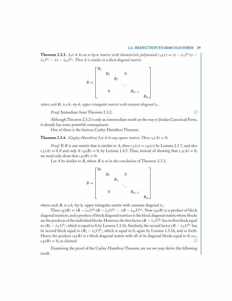
Theorem 2.3.3. Let A be an n-by-n matrix with characteristic polynomial cA(x) = (x − λ1)k1(x −
λ2)k2 · · · (x − λm)km . Then A is similar to a block diagonal matrix
B =
⎡⎢⎢⎢⎢⎢⎢⎢⎣
B1
B2 0B3
. . .
0 Bm−1
Bm
⎤⎥⎥⎥⎥⎥⎥⎥⎦
where each Bi is a ki-by-ki upper triangular matrix with constant diagonal λi .
Proof. Immediate from Theorem 2.3.2.
Although Theorem 2.3.2 is only an intermediate result on the way to Jordan Canonical Form,it already has some powerful consequences.
One of these is the famous Cayley-Hamilton Theorem.
Theorem 2.3.4. (Cayley-Hamilton) Let A be any square matrix. Then cA(A) = 0.
Proof. If B is any matrix that is similar to A, then cA(x) = cB(x) by Lemma 2.1.7, and alsocA(A) = 0 if and only if cB(B) = 0, by Lemma 1.4.5. Thus, instead of showing that cA(A) = 0,we need only show that cB(B) = 0.
Let A be similar to B, where B is as in the conclusion of Theorem 2.3.3,
B =
⎡⎢⎢⎢⎢⎢⎢⎢⎣
B1
B2 0B3
. . .
0 Bm−1
Bm
⎤⎥⎥⎥⎥⎥⎥⎥⎦
where each Bi is a ki-by-ki upper triangular matrix with constant diagonal λi .Then cB(B) = (B − λ1I )k1(B − λ2I )k2 · · · (B − λmI)km . Now cB(B) is a product of block
diagonal matrices, and a product of block diagonal matrices is the block diagonal matrix whose blocksare the products of the individual blocks.However, the first factor (B − λ1I )k1 has its first block equalto (B1 − λ1I )k1 , which is equal to 0, by Lemma 1.3.16. Similarly, the second factor (B − λ2I )k2 hasits second block equal to (B2 − λ2I )k1 , which is equal to 0, again by Lemma 1.3.16, and so forth.Hence the product cB(B) is a block diagonal matrix with all of its diagonal blocks equal to 0, i.e.,cB(B) = 0, as claimed.
Examining the proof of the Cayley-Hamilton Theorem, we see we may derive the followingresult.

30 CHAPTER 2. THE STRUCTURE OF A LINEAR TRANSFORMATION
Corollary 2.3.5. Let A be an n-by-n matrix with distinct eigenvalues λ1, . . ., λm. Let E∞(λi) bethe generalized eigenspace of λi , for each i. Then {E∞(λ1), . . . , E∞(λm)} is a complementary set ofA-invariant subspaces of C
n. In this situation, Cn is the direct sum V = E∞(λ1) ⊕ . . . ⊕ E∞(λm).
Proof. Let A = PBP −1 as in Theorem 2.3.3 and let B be the basis of Cn consisting of the
columns of P .Write B = B1 ∪ . . . ∪ Bm,where B1 consists of the first m1 vectors in B,B2 consists ofthe next m2 vectors in B, etc. Let Wi be the subspace of C
n spanned by Bi . Certainly {W1, . . . , Wm}is a complementary set of subspaces of C
n, and so Cn = W1 ⊕ . . . ⊕ Wm. We claim that in fact
Wi = E∞(λi), for each i, which completes the proof. (Note that each E∞(λi) is A-invariant, byLemma 2.1.17. But also, we can see directly that each Wi is A-invariant, by Lemma 1.5.8.)
To see this claim, let Ti be the restriction of T = TA to Wi . Then Bi = [Ti]Bi. Now Bi is a
ki-by-ki upper triangular matrix with constant diagonal λi , so, by Lemma 1.3.16, (Bi − λiI )ki = 0.Thus any vector wi in Wi is in Eki
(λi) = E∞(λi), i.e., Wi ⊆ E∞(λi). On the other hand, if v
in V is not in Wi , then, writing v = w1 + . . . + wm, with wj in Wj for each j , there must besome value of j = i with wj = 0. But (Bj − λiI ) is a block upper triangular matrix with constantdiagonal λj − λi = 0, so in particular (Bj − λiI ) is nonsingular, as is any of its powers. Hence(Tj − λiI)kwj = 0 no matter what k is. But then also (T − λiI)kv = 0. Thus E∞(λi) ⊆ Wi , andhence these two subspaces are the same.
The next consequence of Theorem 2.3.2 is the relationship between the minimum polynomialmA(x) and the characteristic polynomial cA(x).
Theorem 2.3.6. For any square matrix A:
(1) mA(x) and cA(x) have the same irreducible factors; and
(2) mA(x) divides cA(x).
Proof. We proved (1) in Theorem 2.2.10. By the Cayley-Hamilton Theorem, cA(A) = 0, so(2) follows immediately from Proposition 2.2.7.
Corollary 2.3.7. Let A be an n-by-n matrix. Then mA(x) is a polynomial of degree at most n.
Proof. By Theorem 2.3.6, mA(x) divides cA(x), and cA(x) is a polynomial of degree n.
Let us now restate Theorem 2.3.6 in a more handy form.
Corollary 2.3.8. Let A be a square matrix with characteristic polynomial cA(x) = (x − λ1)k1(x −
λ2)k2 · · · (x − λm)km . Then A has minimum polynomial mA(x) = (x − λ1)
j1(x − λ2)j2 · · · (x −
λm)jm for some integers j1, j2, . . ., jm with 1 ≤ ji ≤ ki for each i.
Proof. Immediate from Theorem 2.3.6.
This corollary has two special cases that are worth stating separately.
2.4. THE DIAGONALIZABLE CASE 31
Corollary 2.3.9. Let A be a square matrix with distinct eigenvalues λ1, . . .,λn.Then mA(x) = cA(x) =(x − λ1)(x − λ2) · · · (x − λn).
Proof. Immediate from Corollary 2.3.8.
Corollary 2.3.10. Let A be an n-by-n square matrix. The following are equivalent:
(1) cA(x) = (x − λ)n for some λ; and
(2) mA(x) = (x − λ)k for some λ and for some k ≤ n.
Proof. Immediate from Corollary 2.3.8.
Here are two final consequences of Theorem 2.3.2.
Corollary 2.3.11. Let A be a square matrix and let λ be an eigenvalue of A. Then the dimension of thegeneralized eigenspace of λ is equal to the algebraic multiplicity alg-mult(λ).
Proof. Examining the proof of Corollary 2.3.5, we see that Wi = E∞(λi) has dimensionmi = alg-mult(λi), for any i.
Corollary 2.3.12. Let A be a square matrix with minimum polynomial mA(x) = (x − λ1)j1(x −
λ2)j2 · · · (x − λm)jm . Then ji = max-ind(λi) for each i,
Proof. Examining the proof of the Cayley-Hamilton Theorem, we see that ji is the smallestexponent such that the block (Bi − λiI )ji = 0. But, in the notation of the proof of Corollary 2.3.5,Wi is the generalized eigenspace of A associated to the eigenvalue λi , so ji is the smallest exponentsuch that (A − λiI )jiw = 0 for every generalized eigenvector w associated to the eigenvalue λi , andby definition that is max-ind(λi).
2.4 THE DIAGONALIZABLE CASEWe pause in our general development of Jordan Canonical Form to consider the important specialcase of diagonalizable matrices, or diagonalizable linear transformations.
Definition 2.4.1. Let A be an n-by-n square matrix. Then A is diagonalizable if A is similar to adiagonal matrix B. �Theorem 2.4.2. Let A be a square matrix with characteristic polynomial cA(x) =(x − λ1)
k1(x − λ2)k2 · · · (x − λm)km . The following are equivalent:
(1) A is diagonalizable.

32 CHAPTER 2. THE STRUCTURE OF A LINEAR TRANSFORMATION
(2a) For each eigenvalue λi of A, geom-mult(λi) = alg-mult(λi).
(2b) For each eigenvalue λi of A, E∞(λi) = E1(λi).
(2c) For each eigenvalue λi of A, max-ind(λi) = 1.
(2d) geom-mult(λ1) + . . . + geom-mult(λk) = n.
(3) The minimum polynomial mA(x) of A is a product of distinct linear factors, cA(x) = (x −λ1)(x − λ2) · · · (x − λm).
Proof. First let us see that conditions (2a), (2b), (2c), and (2d) are all equivalent.We know that E1(λi) is a subspace of E∞(λi), so these two subspaces of C
n are equal ifand only if they have the same dimension. But by definition E1(λi) has dimension geom-mult(λi),and by Corollary 2.3.11 E∞(λi) has dimension alg-mult(λi).Thus (2a) and (2b) are equivalent. ButE∞(λi) = E1(λi) if and only if every generalized eigenvector of A associated to the eigenvalue λi is infact an eigenvector of A, i.e., if and only if max-ind(λi) = 1, so (2b) and (2c) are equivalent. Also, 1 ≤geom-mult(λi) ≤ alg-mult(λi) for each i, and we know that alg-mult(λ1) + . . . + alg-mult(λk) =n, so geom-mult(λ1) + . . . + geom-mult(λk) = n if and only if geom-mult(λi) = alg-mult(λi) foreach i, so (2d) and (2a) are equivalent.
Furthermore, (2c) and (3) are equivalent by Corollary 2.3.12.Now we must relate all these equivalent conditions to diagonalizability.Suppose that A is diagonalizable, A = PBP −1. Since cB(x) = cA(x), B must be a diagonal
matrix with ki entries of λi , for each i. We may assume (after conjugating by a further matrix, ifnecessary), that the entries appear in that order, so we may regard B as being a BDBSM matrix (i.e.,a block diagonal matrix with blocks scalar matrices), where the ith block Bi is the ki-by-ki scalarmatrix Bi = λiI . If B is the basis of C
n consisting of the columns of P , and W1 is the subspace ofC
n spanned by the first k1 columns of P , W2 is the subspace of Cn spanned by the next k2 columns
of P , etc., then Wi = E∞(λi) = E1(λi) for each i.On the other hand, suppose that E∞(λi) = E1(λi) for each i. Then V = E∞(λ1) ⊕ . . . ⊕
E∞(λm) = E1(λ1) ⊕ . . . ⊕ E1(λm). Let P be the matrix whose first k1 columns are a basis forE1(λ1), whose next k2 columns are a basis for E1(λ1), etc. Since Av = λiv for every vector v inE1(λi), we see that A = PBP −1 where B is the BDBSM matrix with diagonal blocks B1, . . ., Bm,where Bi is the ki-by-ki scalar matrix Bi = λiI . In particular, B is a diagonal matrix.
There is an important special case when diagonalizability is automatic.
Corollary 2.4.3. Let A be a square matrix with distinct eigenvalues. Then A is diagonalizable.
Proof. Immediate from Theorem 2.4.2 and Corollary 2.3.9.
Translated from matrices into linear transformations, we obtain the following results:
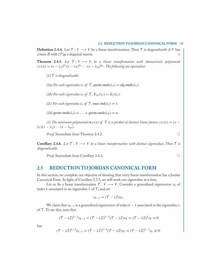
2.5. REDUCTION TO JORDAN CANONICAL FORM 33
Definition 2.4.4. Let T : V −→ V be a linear transformation. Then T is diagonalizable if V hasa basis B with [T ]B a diagonal matrix. �Theorem 2.4.5. Let T : V −→ V be a linear transformation with characteristic polynomialcT (x) = (x − λ1)
k1(x − λ2)k2 · · · (x − λm)km . The following are equivalent:
(1) T is diagonalizable.
(2a) For each eigenvalue λi of T , geom-mult(λi) = alg-mult(λi).
(2b) For each eigenvalue λi of T , E∞(λi) = E1(λi).
(2c) For each eigenvalue λi of T , max-ind(λi) = 1.
(2d) geom-mult(λ1) + . . . + geom-mult(λk) = n.
(3) The minimum polynomial mT (x) of T is a product of distinct linear factors, cT (x) = (x −λ1)(x − λ2) · · · (x − λm).
Proof. Immediate from Theorem 2.4.2.
Corollary 2.4.6. Let T : V −→ V be a linear transformation with distinct eigenvalues. Then T isdiagonalizable.
Proof. Immediate from Corollary 2.4.3.
2.5 REDUCTION TO JORDAN CANONICAL FORMIn this section, we complete our objective of showing that every linear transformation has a JordanCanonical Form. In light of Corollary 2.3.5, we will work one eigenvalue at a time.
Let us fix a linear transformation T : V −→ V . Consider a generalized eigenvector vk ofindex k associated to an eigenvalue λ of T , and set
vk−1 = (T − λI)vk.
We claim that vk−1 is a generalized eigenvector of index k − 1 associated to the eigenvalue λ
of T . To see this, note that
(T − λI)k−1vk−1 = (T − λI)k−1(T − λI)vk = (T − λI)kvk = 0
but(T − λI)k−2vk−1 = (T − λI)k−2(T − λI)vk = (T − λI)k−1vk = 0.
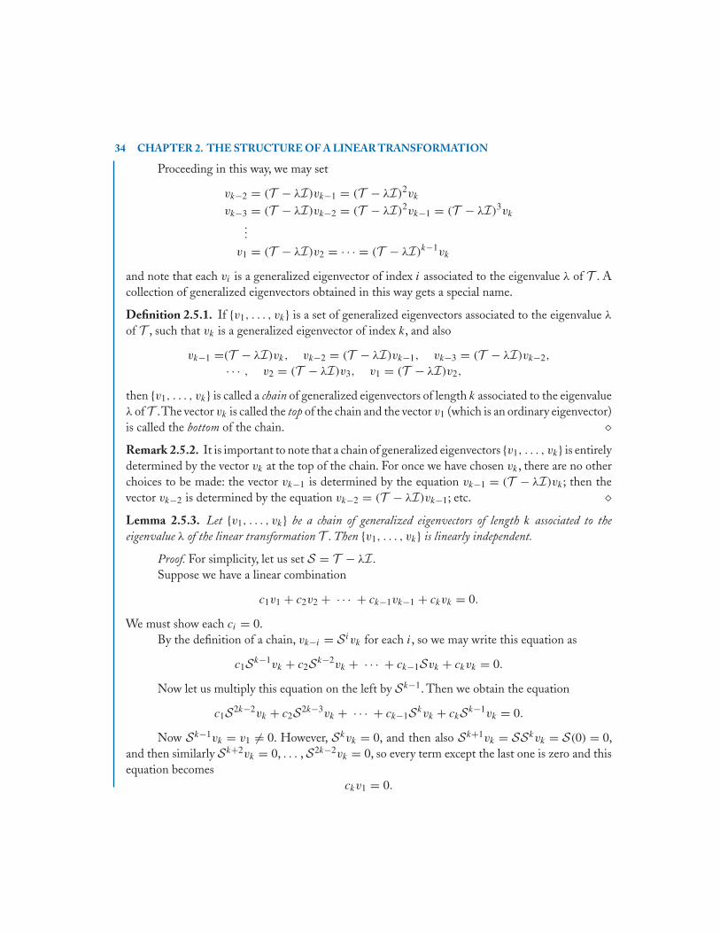
34 CHAPTER 2. THE STRUCTURE OF A LINEAR TRANSFORMATION
Proceeding in this way, we may set
vk−2 = (T − λI)vk−1 = (T − λI)2vk
vk−3 = (T − λI)vk−2 = (T − λI)2vk−1 = (T − λI)3vk
...
v1 = (T − λI)v2 = · · · = (T − λI)k−1vk
and note that each vi is a generalized eigenvector of index i associated to the eigenvalue λ of T . Acollection of generalized eigenvectors obtained in this way gets a special name.
Definition 2.5.1. If {v1, . . . , vk} is a set of generalized eigenvectors associated to the eigenvalue λ
of T , such that vk is a generalized eigenvector of index k, and also
vk−1 =(T − λI)vk, vk−2 = (T − λI)vk−1, vk−3 = (T − λI)vk−2,
· · · , v2 = (T − λI)v3, v1 = (T − λI)v2,
then {v1, . . . , vk} is called a chain of generalized eigenvectors of length k associated to the eigenvalueλ of T .The vector vk is called the top of the chain and the vector v1 (which is an ordinary eigenvector)is called the bottom of the chain. �Remark 2.5.2. It is important to note that a chain of generalized eigenvectors {v1, . . . , vk} is entirelydetermined by the vector vk at the top of the chain. For once we have chosen vk , there are no otherchoices to be made: the vector vk−1 is determined by the equation vk−1 = (T − λI)vk ; then thevector vk−2 is determined by the equation vk−2 = (T − λI)vk−1; etc. �Lemma 2.5.3. Let {v1, . . . , vk} be a chain of generalized eigenvectors of length k associated to theeigenvalue λ of the linear transformation T . Then {v1, . . . , vk} is linearly independent.
Proof. For simplicity, let us set S = T − λI .Suppose we have a linear combination
c1v1 + c2v2 + · · · + ck−1vk−1 + ckvk = 0.
We must show each ci = 0.By the definition of a chain, vk−i = S ivk for each i, so we may write this equation as
c1Sk−1vk + c2Sk−2vk + · · · + ck−1Svk + ckvk = 0.
Now let us multiply this equation on the left by Sk−1. Then we obtain the equation
c1S2k−2vk + c2S2k−3vk + · · · + ck−1Skvk + ckSk−1vk = 0.
Now Sk−1vk = v1 = 0. However, Skvk = 0, and then also Sk+1vk = SSkvk = S(0) = 0,and then similarly Sk+2vk = 0, . . . , S2k−2vk = 0, so every term except the last one is zero and thisequation becomes
ckv1 = 0.
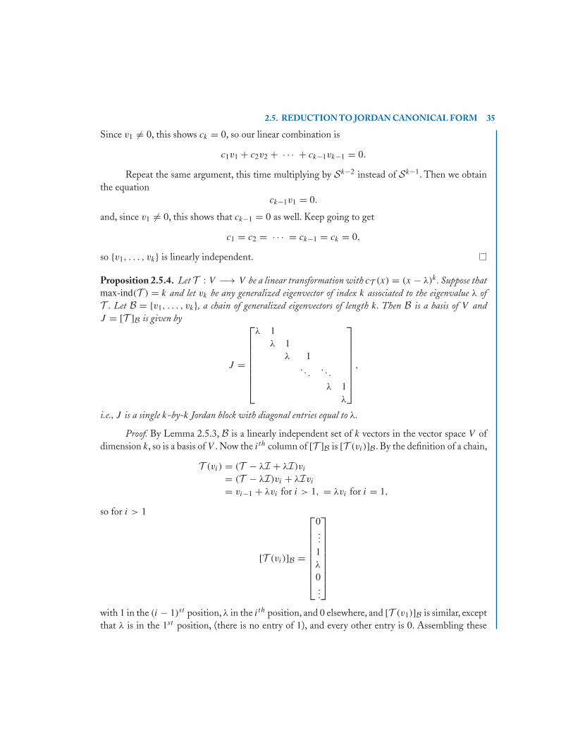
2.5. REDUCTION TO JORDAN CANONICAL FORM 35
Since v1 = 0, this shows ck = 0, so our linear combination is
c1v1 + c2v2 + · · · + ck−1vk−1 = 0.
Repeat the same argument, this time multiplying by Sk−2 instead of Sk−1. Then we obtainthe equation
ck−1v1 = 0.
and, since v1 = 0, this shows that ck−1 = 0 as well. Keep going to get
c1 = c2 = · · · = ck−1 = ck = 0,
so {v1, . . . , vk} is linearly independent.
Proposition 2.5.4. Let T : V −→ V be a linear transformation with cT (x) = (x − λ)k . Suppose thatmax-ind(T ) = k and let vk be any generalized eigenvector of index k associated to the eigenvalue λ ofT . Let B = {v1, . . . , vk}, a chain of generalized eigenvectors of length k. Then B is a basis of V andJ = [T ]B is given by
J =
⎡⎢⎢⎢⎢⎢⎢⎢⎣
λ 1λ 1
λ 1. . .
. . .
λ 1λ
⎤⎥⎥⎥⎥⎥⎥⎥⎦
,
i.e., J is a single k-by-k Jordan block with diagonal entries equal to λ.
Proof. By Lemma 2.5.3, B is a linearly independent set of k vectors in the vector space V ofdimension k, so is a basis of V . Now the ith column of [T ]B is [T (vi)]B. By the definition of a chain,
T (vi) = (T − λI + λI)vi
= (T − λI)vi + λIvi
= vi−1 + λvi for i > 1, = λvi for i = 1,
so for i > 1
[T (vi)]B =
⎡⎢⎢⎢⎢⎢⎢⎢⎢⎣
0...
1λ
0...
⎤⎥⎥⎥⎥⎥⎥⎥⎥⎦
with 1 in the (i − 1)st position, λ in the ith position, and 0 elsewhere, and [T (v1)]B is similar, exceptthat λ is in the 1st position, (there is no entry of 1), and every other entry is 0. Assembling these

36 CHAPTER 2. THE STRUCTURE OF A LINEAR TRANSFORMATION
vectors, and recalling Definition 1.3.11, we see that the matrix J = [T ]B has the form of a singlek-by-k Jordan block with diagonal entries equal to λ.
Here is the goal to which we have been heading. Before stating this theorem, we recall fromDefinition 1.3.12 that a matrix in Jordan Canonical Form is a block diagonal matrix, with each blocka Jordan block.
Theorem 2.5.5. Let V be a vector space and let T : V −→ V be a linear transformation. Then V has abasis B in which A = [T ]B is a matrix in Jordan Canonical Form.
Proof. Let V have dimension n. We prove this by complete induction on n.
If n = 1, then the only possible linear transformation T is T (v) = λv for some λ, and then,in any basis B, [T ]B is the 1-by-1 matrix [λ], which is certainly in Jordan Canonical Form.
Now for the inductive step. In the course of this argument, we will sometimes be explicitlychanging bases, and sometimes conjugating by nonsingular matrices. Of course, these have the sameeffect (cf. Remark 1.2.12), but sometimes one will be more convenient than the other.
As a first step, we know by Theorem 2.3.1 that V has a basis C with [T ]C a ma-trix in BDBUTCD form. More precisely, let cT (x) = (x − λ1)
k1(x − λ2)k2 · · · (x − λm)km . Let
Wi = E∞(λi), for each i. We may write C = C1 ∪ . . . ∪ Cm where Ci is a basis of Wi , for eachi. Let Ti denote the restriction of T to Wi .
First, consider W1 and T1. Let k = k1. Let j = j1 = max-ind(λ1). Choose a generalizedeigenvector wj of index j in W1 and form a chain of generalized eigenvectors D1,1 = {w1, . . . , wj }.This set is a basis for a subspace W1,1 of W1. If j1 = k1 then W1,1 = W1 and D1,1 is a basis for W1.In that case, we set B1 = D1,1, and we are finished with the eigenvalue λ1. Otherwise, let W1,2 bea complement of W1,1 in W1, and let D1,2 be a basis for W1,2. Let D = D1,1 ∪ D1,2. Finally, letT1,1 be the restriction of T1 to W1,1. By Proposition 2.5.4, we know that [T1,1]D1,1 = J1 is a j-by-jJordan block with diagonal entries of λ1. Furthermore, by Lemma 1.5.8, we also know that [T ]D isa block upper triangular matrix,
Q = [T ]D =[J1 B
0 D
],
where B is a j-by-(k − j) matrix and D is an (k − j)-by-(k − j) matrix.We now apply the inductivehypothesis to conclude that there is a (k − j)-by-(k − j) matrix P0 such that H = PDP −1 is inJordan Canonical Form (with all diagonal entries equal to λ1). Let P be the n-by-n block diagonalmatrix
P =[I 00 P0
].
Then direct computation shows that
R = PQP −1 =[J1 F
0 H
],
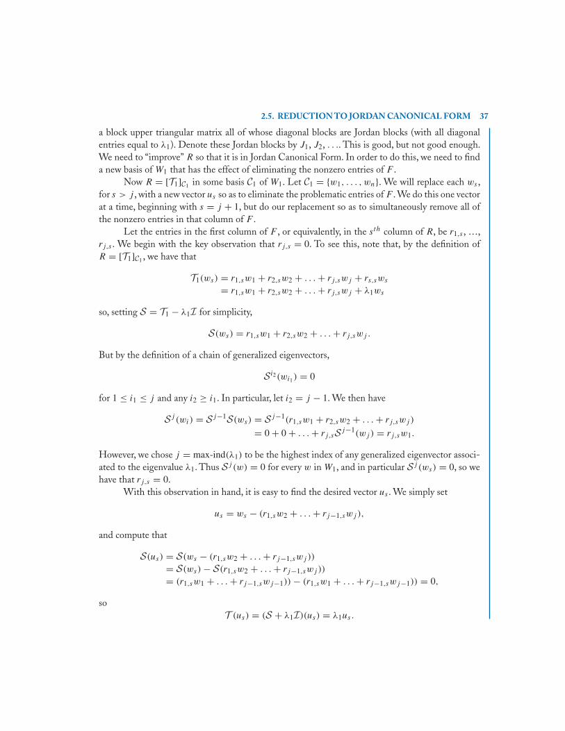
2.5. REDUCTION TO JORDAN CANONICAL FORM 37
a block upper triangular matrix all of whose diagonal blocks are Jordan blocks (with all diagonalentries equal to λ1). Denote these Jordan blocks by J1, J2, . . .. This is good, but not good enough.We need to “improve” R so that it is in Jordan Canonical Form. In order to do this, we need to finda new basis of W1 that has the effect of eliminating the nonzero entries of F .
Now R = [T1]C1 in some basis C1 of W1. Let C1 = {w1, . . . , wn}. We will replace each ws ,for s > j , with a new vector us so as to eliminate the problematic entries of F . We do this one vectorat a time, beginning with s = j + 1, but do our replacement so as to simultaneously remove all ofthe nonzero entries in that column of F .
Let the entries in the first column of F , or equivalently, in the sth column of R, be r1,s , …,rj,s . We begin with the key observation that rj,s = 0. To see this, note that, by the definition ofR = [T1]C1 , we have that
T1(ws) = r1,sw1 + r2,sw2 + . . . + rj,swj + rs,sws
= r1,sw1 + r2,sw2 + . . . + rj,swj + λ1ws
so, setting S = T1 − λ1I for simplicity,
S(ws) = r1,sw1 + r2,sw2 + . . . + rj,swj .
But by the definition of a chain of generalized eigenvectors,
S i2(wi1) = 0
for 1 ≤ i1 ≤ j and any i2 ≥ i1. In particular, let i2 = j − 1. We then have
Sj (wi) = Sj−1S(ws) = Sj−1(r1,sw1 + r2,sw2 + . . . + rj,swj )
= 0 + 0 + . . . + rj,sSj−1(wj ) = rj,sw1.
However, we chose j = max-ind(λ1) to be the highest index of any generalized eigenvector associ-ated to the eigenvalue λ1. Thus Sj (w) = 0 for every w in W1, and in particular Sj (ws) = 0, so wehave that rj,s = 0.
With this observation in hand, it is easy to find the desired vector us . We simply set
us = ws − (r1,sw2 + . . . + rj−1,swj ),
and compute that
S(us) = S(ws − (r1,sw2 + . . . + rj−1,swj ))
= S(ws) − S(r1,sw2 + . . . + rj−1,swj ))
= (r1,sw1 + . . . + rj−1,swj−1)) − (r1,sw1 + . . . + rj−1,swj−1)) = 0,
soT (us) = (S + λ1I)(us) = λ1us.

38 CHAPTER 2. THE STRUCTURE OF A LINEAR TRANSFORMATION
Thus in the basis C′1 = {w1, . . . , wj , uj+1, wj+2, . . . , wk} of W1, we have [T1]C′
1= R′ is a matrix
R′ =[J1 F ′0 H
],
where J1 and H are as before, but now every entry in the first column of F ′ is 0. Continue in thisfashion to obtain a basis B1 of W1 with [T1]B1 of the form
[J1 00 H
],
a matrix in Jordan Canonical Form with all diagonal entries equal to λ1.This takes care of the generalized eigenspace W1 = E∞(λ1). Perform the same process for
each generalized eigenspace Wi , obtaining a basis Bi with [Ti]Biin Jordan Canonical Form, for each
i. Then, if B = B1 ∪ . . . ∪ Bm, we have that A = [T ]B is a matrix in Jordan Canonical Form.
(Observe in the proof that it was crucial that we started with the longest chain when workingwith each eigenvalue.)
Again, we proved a more precise result than we have stated. Let us state that more preciseresult now.
Theorem 2.5.6. Let V be a vector space and let T : V −→ V be a linear transformation withcharacteristic polynomial cT (x) = (x − λ1)
k1(x − λ2)k2 · · · (x − λm)km . and minimum polynomial
mT (x) = (x − λ1)j1(x − λ2)
j2 · · · (x − λm)jm . Then V has a basis B in which J = [T ]B is a matrixin Jordan Canonical Form
J =
⎡⎢⎢⎢⎢⎢⎢⎢⎣
J1
J2 0J3
. . .
0 Jp−1
Jp
⎤⎥⎥⎥⎥⎥⎥⎥⎦
,
where J1, . . ., Jp are all Jordan blocks.
Furthermore, for each i:
(1) the sum of the sizes of the Jordan blocks with diagonal entries λi is equal to ki = alg-mult(λi);
(2) the largest Jordan block with diagonal entries λi is ji-by-ji where ji = max-ind(λi); and
(3) the number of Jordan blocks with diagonal entries λi is equal to geom-mult(λi).
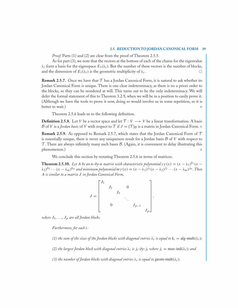
2.5. REDUCTION TO JORDAN CANONICAL FORM 39
Proof. Parts (1) and (2) are clear from the proof of Theorem 2.5.5.As for part (3), we note that the vectors at the bottom of each of the chains for the eigenvalue
λi form a basis for the eigenspace E1(λi). But the number of these vectors is the number of blocks,and the dimension of E1(λi) is the geometric multiplicity of λi .
Remark 2.5.7. Once we have that T has a Jordan Canonical Form, it is natural to ask whether itsJordan Canonical Form is unique. There is one clear indeterminacy, as there is no a priori order tothe blocks, so they can be reordered at will. This turns out to be the only indeterminacy. We willdefer the formal statement of this to Theorem 3.2.9, when we will be in a position to easily prove it.(Although we have the tools to prove it now, doing so would involve us in some repetition, so it isbetter to wait.) �
Theorem 2.5.6 leads us to the following definition.
Definition 2.5.8. Let V be a vector space and let T : V −→ V be a linear transformation. A basisB of V is a Jordan basis of V with respect to T if J = [T ]B is a matrix in Jordan Canonical Form. �Remark 2.5.9. As opposed to Remark 2.5.7, which states that the Jordan Canonical Form of Tis essentially unique, there is never any uniqueness result for a Jordan basis B of V with respect toT . There are always infinitely many such bases B. (Again, it is convenient to delay illustrating thisphenomenon.) �
We conclude this section by restating Theorem 2.5.6 in terms of matrices.
Theorem 2.5.10. Let A be an n-by-n matrix with characteristic polynomial cT (x) = (x − λ1)k1(x −
λ2)k2 · · · (x − λm)km and minimum polynomial mT (x) = (x − λ1)
j1(x − λ2)j2 · · · (x − λm)jm . Then
A is similar to a matrix J in Jordan Canonical Form,
J =
⎡⎢⎢⎢⎢⎢⎢⎢⎣
J1
J2 0J3
. . .
0 Jp−1
Jp
⎤⎥⎥⎥⎥⎥⎥⎥⎦
,
where J1, . . ., Jp are all Jordan blocks.
Furthermore, for each i:
(1) the sum of the sizes of the Jordan blocks with diagonal entries λi is equal to ki = alg-mult(λi);
(2) the largest Jordan block with diagonal entries λi is ji-by-ji where ji = max-ind(λi); and
(3) the number of Jordan blocks with diagonal entries λi is equal to geom-mult(λi).
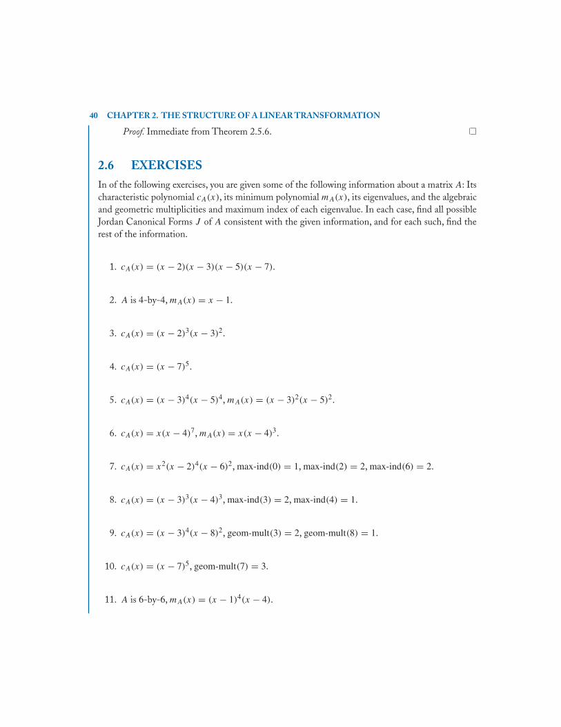
40 CHAPTER 2. THE STRUCTURE OF A LINEAR TRANSFORMATION
Proof. Immediate from Theorem 2.5.6.
2.6 EXERCISESIn of the following exercises, you are given some of the following information about a matrix A: Itscharacteristic polynomial cA(x), its minimum polynomial mA(x), its eigenvalues, and the algebraicand geometric multiplicities and maximum index of each eigenvalue. In each case, find all possibleJordan Canonical Forms J of A consistent with the given information, and for each such, find therest of the information.
1. cA(x) = (x − 2)(x − 3)(x − 5)(x − 7).
2. A is 4-by-4, mA(x) = x − 1.
3. cA(x) = (x − 2)3(x − 3)2.
4. cA(x) = (x − 7)5.
5. cA(x) = (x − 3)4(x − 5)4, mA(x) = (x − 3)2(x − 5)2.
6. cA(x) = x(x − 4)7, mA(x) = x(x − 4)3.
7. cA(x) = x2(x − 2)4(x − 6)2, max-ind(0) = 1, max-ind(2) = 2, max-ind(6) = 2.
8. cA(x) = (x − 3)3(x − 4)3, max-ind(3) = 2, max-ind(4) = 1.
9. cA(x) = (x − 3)4(x − 8)2, geom-mult(3) = 2, geom-mult(8) = 1.
10. cA(x) = (x − 7)5, geom-mult(7) = 3.
11. A is 6-by-6, mA(x) = (x − 1)4(x − 4).

2.6. EXERCISES 41
12. A is 6-by-6, mA(x) = (x − 2)2(x − 3).
13. alg-mult(1) = 5, geom-mult(1) = 3.
14. alg-mult(2) = 6, geom-mult(2) = 3.
15. alg-mult(3) = 5, max-ind(3) = 2.
16. alg-mult(4) = 6, max-ind(4) = 3.
17. alg-mult(8) = 6, geom-mult(8) = 3, max-ind(8) = 4.
18. alg-mult(9) = 6, geom-mult(4) = 4, max-ind(4) = 2.
19. (a) Suppose A is an n-by-n matrix with n ≤ 3. Show that A is determined up to similarity byits characteristic polynomial and its minimum polynomial.
(b) Show by example that this is not true if n = 4.
20. (a) Suppose A is an n-by-n matrix with n ≤ 3. Show that A is determined up to similarity byits characteristic polynomial and the geometric multiplicities of each of its eigenvalues.
(b) Show by example that this is not true if n = 4.
21. (a) Suppose A is an n-by-n matrix with n ≤ 6. Show that A is determined up to similarityby its characteristic polynomial, its minimum polynomial, and the geometric multiplicities ofeach of its eigenvalues.
(b) Show by example that this is not true if n = 7.
22. For n ≥ 2 and b = 0, let M = Mn(a, b) be the n-by-n matrix all of whose diagonal entriesare equal to a and all of whose off-diagonal entries are equal to b.

42 CHAPTER 2. THE STRUCTURE OF A LINEAR TRANSFORMATION
(a) Show that a − b is an eigenvalue of M of geometric multiplicity n − 1.
(b) Show that a + (n − 1)b is an eigenvalue of M of geometric multiplicity 1.
(c) Use the results of parts (a) and (b) to find the characteristic polynomial cM(x) and theminimum polynomial mM(x).
(d) Find the Jordan Canonical Form J of M and an invertible matrix P with M = PJP −1.

43
C H A P T E R 3
An Algorithm forJordan Canonical Form
and Jordan BasisOur objective in this chapter is to develop an algorithm for finding the JCF of a linear transfor-mation, assuming that one can find its eigenvalues, i.e., that one can factor its characteristic (orminimum) polynomial. We will further develop the algorithm to find a Jordan basis as well. Webegin this development by defining the eigenstructure picture (or ESP) of a linear transformation,which represents its JCF in an way that is easy to visualize. Then we develop the algorithm per se,and illustrate it with many examples.
3.1 THE ESP OF A LINEAR TRANSFORMATIONIn this section,we present the eigenstructure picture,or ESP,of a linear transformationT : V −→ V .
Part of our discussion will be general, but we shall also proceed partly by example, as to proceedin complete generality would lead to a blizzard of subscripts, which would only confuse the issue.But our examples should be general enough to make the situation clear.
Here is the basic element of an ESP :
Construction 3.1.1. Let T : V −→ V be a linear transformation and let λ be an eigenvalue ofT . Suppose that T has a chain of generalized eigenvectors (see Definition 2.5.1) {v1, . . . , vk} oflength k associated to the eigenvector λ. In this situation, we have the following “labelled picture”in Figure 3.1.
By way of explanation, each integer on the left denote the index of the relevant generalizedeigenvector. Each node represents a generalized eigenvector of that index, so in this picture, indexis synonymous with height (with the lowest level being at height 1). The solid links between thenodes indicate that these generalized eigenvectors are all part of a chain.The complex number at thebottom is the associated eigenvalue. Finally, each node is labelled with the corresponding generalizedeigenvector.
In this situation, we also have the “unlabelled picture” (or simply “picture”), which is obtainedfrom the labelled picture simply by deleting all the labels. �
We will often think of Construction 3.1.1 the other way around. That is, we will think ofbeginning with the picture and obtaining the labelled picture from it by adding labels to all thenodes.

44 CHAPTER 3. AN ALGORITHM FOR JORDAN CANONICAL FORM AND JORDAN BASIS
vk
vk-1 k-1
v2
v
2
1l
1
k
Figure 3.1.
Construction 3.1.2. Let T : V −→ V be a linear transformation. The eigenstructure picture, orESP, of T is the picture obtained by writing down all the pictures of its various chains next to eachother. (We only write the indices once, to avoid duplication.)
The labelled eigenstructure picture, or �ESP , of T is the picture obtained by writing down allthe labelled pictures of its various chains next to each other (again, with the indices only writtenonce, to avoid duplication).
We call a node in a column associated to an eigenvalue λ a λ-node. �
Example 3.1.3. (1) Let T : V −→ V be a linear transformation with ESP the picture in Figure 3.1.Then the JCF J of T is a single k-by-k Jordan block,
J =
⎡⎢⎢⎢⎢⎢⎢⎢⎣
λ 1λ 1
λ 1. . .
. . .
λ 1λ
⎤⎥⎥⎥⎥⎥⎥⎥⎦
.
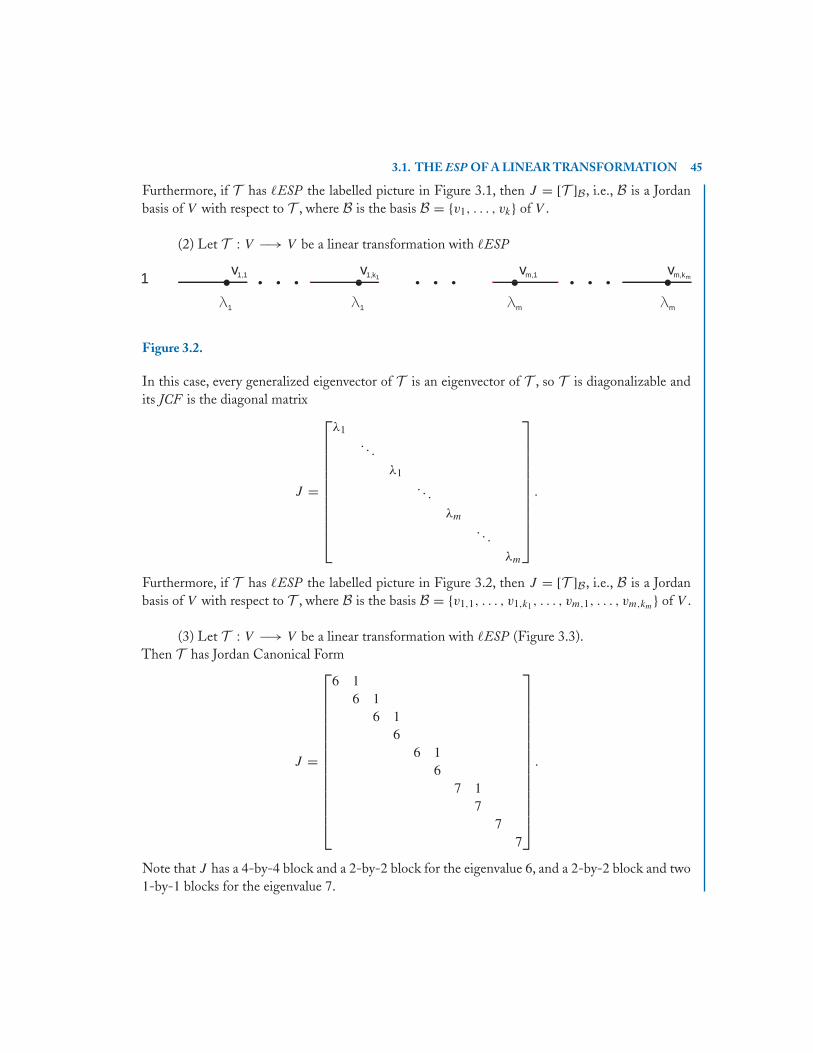
3.1. THE ESP OF A LINEAR TRANSFORMATION 45
Furthermore, if T has �ESP the labelled picture in Figure 3.1, then J = [T ]B, i.e., B is a Jordanbasis of V with respect to T , where B is the basis B = {v1, . . . , vk} of V .
(2) Let T : V −→ V be a linear transformation with �ESP
v1,1
l
1
1
v1,k1
l1
vm,1
lm
vm,km
lm
Figure 3.2.
In this case, every generalized eigenvector of T is an eigenvector of T , so T is diagonalizable andits JCF is the diagonal matrix
J =
⎡⎢⎢⎢⎢⎢⎢⎢⎢⎢⎢⎢⎣
λ1. . .
λ1. . .
λm
. . .
λm
⎤⎥⎥⎥⎥⎥⎥⎥⎥⎥⎥⎥⎦
.
Furthermore, if T has �ESP the labelled picture in Figure 3.2, then J = [T ]B, i.e., B is a Jordanbasis of V with respect to T , where B is the basis B = {v1,1, . . . , v1,k1, . . . , vm,1, . . . , vm,km} of V .
(3) Let T : V −→ V be a linear transformation with �ESP (Figure 3.3).Then T has Jordan Canonical Form
J =
⎡⎢⎢⎢⎢⎢⎢⎢⎢⎢⎢⎢⎢⎢⎢⎢⎣
6 16 1
6 16
6 16
7 17
77
⎤⎥⎥⎥⎥⎥⎥⎥⎥⎥⎥⎥⎥⎥⎥⎥⎦
.
Note that J has a 4-by-4 block and a 2-by-2 block for the eigenvalue 6, and a 2-by-2 block and two1-by-1 blocks for the eigenvalue 7.

46 CHAPTER 3. AN ALGORITHM FOR JORDAN CANONICAL FORM AND JORDAN BASIS
v4 4
v3 3
v2 2 w2
w1 x1 y1 z1
x2
v1
6
1
6 7 7 7
Figure 3.3.
Also, B = {v1, v2, v3, v4, w1, w2, x1, x2, y1, z1} is a Jordan basis of V with respect to T .
(4) Let T : V −→ V be a linear transformation with �ESP
v3
v2
v
51
2
3
1 x1 y1 z1
z2
w3
w2
w1
855 5
Figure 3.4.

3.1. THE ESP OF A LINEAR TRANSFORMATION 47
Then T has Jordan Canonical Form
J =
⎡⎢⎢⎢⎢⎢⎢⎢⎢⎢⎢⎢⎢⎢⎢⎢⎣
5 15 1
55 1
5 15
55
8 18
⎤⎥⎥⎥⎥⎥⎥⎥⎥⎥⎥⎥⎥⎥⎥⎥⎦
.
Note that J has two 3-by-3 blocks and two 1-by-1 blocks for the eigenvalue 5, and a 2-by-2 blockfor the eigenvalue 8.
Also, B = {v1, v2, v3, w1, w2, w3, x1, y1, z1, z2} is a Jordan basis of V with respect to T .
(5) Let T : V −→ V be a linear transformation with �ESP
v4
3
2
1
4
v3
v2
v
0
1
w2
w1 x1
y2
y1 z 1
0 0 40
Figure 3.5.

48 CHAPTER 3. AN ALGORITHM FOR JORDAN CANONICAL FORM AND JORDAN BASIS
Then T has Jordan Canonical Form
J =
⎡⎢⎢⎢⎢⎢⎢⎢⎢⎢⎢⎢⎢⎢⎢⎢⎣
0 10 1
0 10
0 10
01 1
14
⎤⎥⎥⎥⎥⎥⎥⎥⎥⎥⎥⎥⎥⎥⎥⎥⎦
.
Note that J has a 4-by-4 block, a 2-by-2 block, and a 1-by-1 block for the eigenvalue 0, a 2-by-2block for the eigenvalue 1, and a 1-by-1 block for the eigenvalue 4.
Also, B = {v1, v2, v3, v4, w1, w2, x1, y1, y2, z1} is a Jordan basis of V with respect to T .�
From Example 3.1.3, it should be clear how to translate between the ESP of a linear trans-formation and its JCF, and that each of these determines the other. It should also be clear how totranslate between an �ESP of a linear transformation and its JCF together with a Jordan basis, andthat each of these determines the other.
Note that we may reorder the columns in the ESP of a linear transformation, and that corre-sponds to reordering the blocks in its JCF.
3.2 THE ALGORITHM FOR JORDAN CANONICAL FORMIn this section, we develop our algorithm. Actually, what we will develop is an algorithm for de-termining the ESP of a linear transformation. In light of the previous section, that determines its JCF.
We fix a linear transformation T : V −→ V .
Let us reestablish some notation. Recall Definition 2.1.14 and Definition 2.1.5 (both restatedin terms of a linear transformation): For an eigenvalue λ of T , and a fixed integer j , we let Ej(λ) bethe set of vectors
Ej(λ) = {v | (T − λI)j v = 0} = Ker((T − λI)j ).
Also, we let E∞(λ) be the set of vectors
E∞(λ) = {v | (T − λI)j v = 0 for some j} = {v | v is in Ej(λ) for some j}.(E∞(λ) is the generalized eigenspace of λ.)
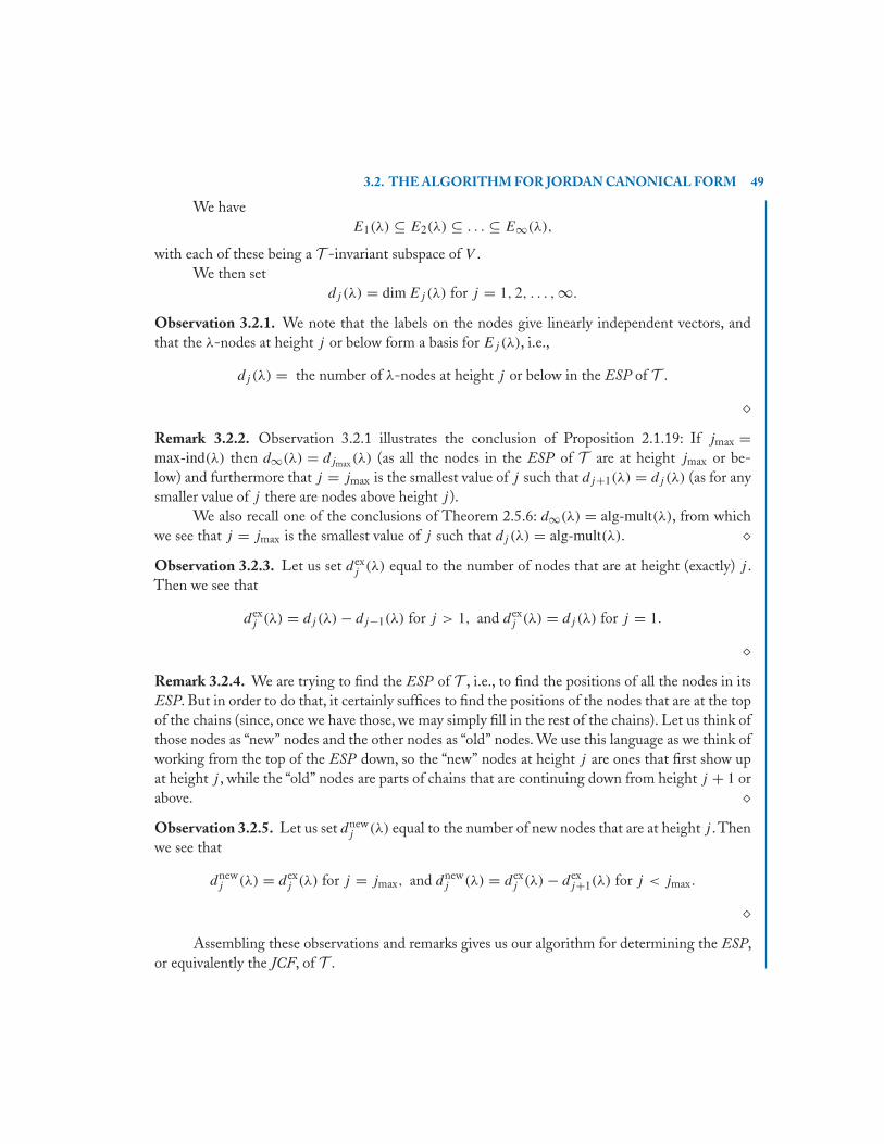
3.2. THE ALGORITHM FOR JORDAN CANONICAL FORM 49
We haveE1(λ) ⊆ E2(λ) ⊆ . . . ⊆ E∞(λ),
with each of these being a T -invariant subspace of V .We then set
dj (λ) = dim Ej(λ) for j = 1, 2, . . . ,∞.
Observation 3.2.1. We note that the labels on the nodes give linearly independent vectors, andthat the λ-nodes at height j or below form a basis for Ej(λ), i.e.,
dj (λ) = the number of λ-nodes at height j or below in the ESP of T .
�Remark 3.2.2. Observation 3.2.1 illustrates the conclusion of Proposition 2.1.19: If jmax =max-ind(λ) then d∞(λ) = djmax(λ) (as all the nodes in the ESP of T are at height jmax or be-low) and furthermore that j = jmax is the smallest value of j such that dj+1(λ) = dj (λ) (as for anysmaller value of j there are nodes above height j ).
We also recall one of the conclusions of Theorem 2.5.6: d∞(λ) = alg-mult(λ), from whichwe see that j = jmax is the smallest value of j such that dj (λ) = alg-mult(λ). �Observation 3.2.3. Let us set dex
j (λ) equal to the number of nodes that are at height (exactly) j .Then we see that
dexj (λ) = dj (λ) − dj−1(λ) for j > 1, and dex
j (λ) = dj (λ) for j = 1.
�Remark 3.2.4. We are trying to find the ESP of T , i.e., to find the positions of all the nodes in itsESP. But in order to do that, it certainly suffices to find the positions of the nodes that are at the topof the chains (since, once we have those, we may simply fill in the rest of the chains). Let us think ofthose nodes as “new” nodes and the other nodes as “old” nodes. We use this language as we think ofworking from the top of the ESP down, so the “new” nodes at height j are ones that first show upat height j , while the “old” nodes are parts of chains that are continuing down from height j + 1 orabove. �Observation 3.2.5. Let us set dnew
j (λ) equal to the number of new nodes that are at height j . Thenwe see that
dnewj (λ) = dex
j (λ) for j = jmax, and dnewj (λ) = dex
j (λ) − dexj+1(λ) for j < jmax.
�Assembling these observations and remarks gives us our algorithm for determining the ESP,
or equivalently the JCF, of T .
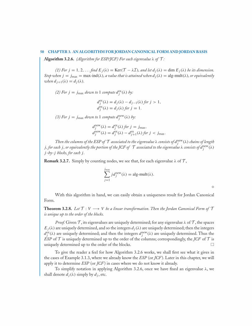
50 CHAPTER 3. AN ALGORITHM FOR JORDAN CANONICAL FORM AND JORDAN BASIS
Algorithm 3.2.6. (Algorithm for ESP/JCF) For each eigenvalue λ of T :
(1) For j = 1, 2, . . . find Ej(λ) = Ker(T − λI), and let dj (λ) = dim Ej(λ) be its dimension.Stop when j = jmax = max-ind(λ), a value that is attained when dj (λ) = alg-mult(λ), or equivalentlywhen dj+1(λ) = dj (λ).
(2) For j = jmax down to 1 compute dexj (λ) by:
dexj (λ) = dj (λ) − dj−1(λ) for j > 1,
dexj (λ) = dj (λ) for j = 1.
(3) For j = jmax down to 1 compute dnewj (λ) by:
dnewj (λ) = dex
j (λ) for j = jmax,
dnewj (λ) = dex
j (λ) − dexj+1(λ) for j < jmax.
Then the columns of the ESP of T associated to the eigenvalue λ consists of dnewj (λ) chains of length
j , for each j , or equivalently the portion of the JCF of T associated to the eigenvalue λ consists of dnewj (λ)
j-by-j blocks, for each j .
Remark 3.2.7. Simply by counting nodes, we see that, for each eigenvalue λ of T ,
jmax∑j=1
jdnewj (λ) = alg-mult(λ).
�With this algorithm in hand, we can easily obtain a uniqueness result for Jordan Canonical
Form.
Theorem 3.2.8. Let T : V −→ V be a linear transformation. Then the Jordan Canonical Form of Tis unique up to the order of the blocks.
Proof. Given T , its eigenvalues are uniquely determined; for any eigenvalue λ of T , the spacesEj(λ) are uniquely determined, and so the integers dj (λ) are uniquely determined; then the integersdexj (λ) are uniquely determined; and then the integers dnew
j (λ) are uniquely determined. Thus theESP of T is uniquely determined up to the order of the columns; correspondingly, the JCF of T isuniquely determined up to the order of the blocks.
To give the reader a feel for how Algorithm 3.2.6 works, we shall first see what it gives inthe cases of Example 3.1.3, where we already know the ESP (or JCF ). Later in this chapter, we willapply it to determine ESP (or JCF ) in cases where we do not know it already.
To simplify notation in applying Algorithm 3.2.6, once we have fixed an eigenvalue λ, weshall denote dj (λ) simply by dj , etc.

3.2. THE ALGORITHM FOR JORDAN CANONICAL FORM 51
Example 3.2.9. (1) Let T be as in Example 3.1.3 (1). Then
dj (λ) = j for j = 1, . . . , k.
Since dk = k = alg-mult(λ) but dj < k = alg-mult(λ) for j < k, we have that jmax = k. Then
dexj (λ) = j − (j − 1) = 1 for j = k, k − 1, . . . , 1,
and thendnewk (λ) = 1 − 0 = 1 and dnew
j (λ) = 1 − 1 = 0 for j = k − 1, . . . , 1.
Thus the ESP of T has 1 chain of length k associated to the eigenvalue λ.
(2) Let T be as in Example 3.1.3 (2). Then for each eigenvalue λi of T ,
d1(λi) = ki.
Since ki = alg-mult(λi), we have that jmax(λi) = 1. Then
dex1 (λi) = ki,
and thendnew
1 (λi) = ki.
Thus the ESP of T has ki chains of length 1 associated to the eigenvalue λi .
(3) Let T be as in Example 3.1.3 (3).For the eigenvalue 6 of T ,
d1 = 2, d2 = 4, d3 = 5, d4 = 6,
and jmax = 4. Then
dex4 = 6 − 5 = 1, dex
3 = 5 − 4 = 1, dex2 = 4 − 2 = 2, dex
1 = 2,
and thendnew
4 = 1, dnew3 = 1 − 1 = 0, dnew
2 = 2 − 1 = 1, dnew1 = 2 − 2 = 0.
Thus the ESP of T has 1 chain of length 4 and 1 chain of length 2 associated to the eigenvalue 6.For the eigenvalue 7 of T ,
d1 = 3, d2 = 4,
and jmax = 2. Thendex
2 = 4 − 3 = 1, dex1 = 3,
and thendnew
2 = 1, dnew1 = 3 − 1 = 2.

52 CHAPTER 3. AN ALGORITHM FOR JORDAN CANONICAL FORM AND JORDAN BASIS
Thus the ESP of T has 1 chain of length 2 and 2 chains of length 1 associated to the eigenvalue 7.
(3) Let T be as in Example 3.1.3 (4).For the eigenvalue 5 of T ,
d1 = 4, d2 = 6, d3 = 8,
and jmax = 3. Thendex
3 = 8 − 6 = 2, dex2 = 6 − 4 = 2, dex
1 = 4,
and thendnew
3 = 2, dnew2 = 2 − 2 = 0, dnew
1 = 4 − 2 = 2.
Thus the ESP of T has 2 chains of length 3 and 2 chains of length 1 associated to the eigenvalue 5.For the eigenvalue 8 of T ,
d1 = 1, d2 = 2,
and jmax = 2. Thendex
2 = 2 − 1 = 1, dex1 = 1,
and thendnew
2 = 1, dnew1 = 1 − 1 = 0.
Thus the ESP of T has 1 chain of length 2 associated to the eigenvalue 8.
(3) Let T be as in Example 3.1.3 (5).For the eigenvalue 0 of T ,
d1 = 3, d2 = 5, d3 = 6, d4 = 7,
and jmax = 4. Then
dex4 = 7 − 6 = 1, dex
3 = 6 − 5 = 1, dex2 = 5 − 3 = 2, dex
1 = 3,
and thendnew
4 = 1, dnew3 = 1 − 1 = 0, dnew
2 = 2 − 1 = 1, dnew1 = 3 − 2 = 1.
Thus the ESP of T has 1 chain of length 4, 1 chain of length 2, and 1 chain of length 1 associatedto the eigenvalue 0.
For the eigenvalue 1 of T ,d1 = 1, d2 = 2,
and jmax = 2. Thendex
2 = 2 − 1 = 1, dex1 = 1,
and thendnew
2 = 1, dnew1 = 1 − 1 = 0.
3.3. THE ALGORITHM FOR A JORDAN BASIS 53
Thus the ESP of T has 1 chain of length 2 associated to the eigenvalue 1.
For the eigenvalue 4 of T ,d1 = 1,
and jmax = 1. Thendex
1 = 1,
and thendnew
1 = 1.
Thus the ESP of T has 1 chain of length 1 associated to the eigenvalue 4. �
3.3 THE ALGORITHM FOR A JORDAN BASISWe continue to fix a linear transformation T : V −→ V .
In this section, we further develop our algorithm in order to obtain a Jordan basis of V
with respect to T . We have already developed an algorithm for determining the ESP of a lineartransformation. Now we will extend our algorithm in order to determine labels on its nodes, andhence a �ESP of T . We can then directly read off a Jordan basis from the labels on the nodes.
We have been careful in our language. As we have already remarked, and as we shall seeconcretely below, there is no uniqueness whatsoever for a Jordan basis, so we will be finding a, notthe, Jordan basis of V with respect to T .
We suppose that we have already found the ESP of T .We will be working one eigenvalue at a time. For each eigenvalue λ, we will be working from
the top down from the top down, that is, starting with jmax = max-ind(λ) and ending with j = 1.Recall Remark 3.2.4: At any stage, that is, for any given value of j , we think of the nodes that are atthe top of chains of height j as “new” nodes, since we see them for the first time at this stage. Theother nodes at height j are parts of chains we have already seen, and so we think of them as “old”nodes. Note that when we first start, with j = jmax, every node at this height is a new node. Ourtask is then to find the labels on the new nodes at each stage.
To clarify this, let us look back at our examples.First, consider Example 3.1.3 (3). For the eigenvalue 6, we start with j = 4 and work our way
down. For j = 4, we have one new node, v4. For j = 3, we have one old node, v3, and no new nodes.For j = 2, we have one old node, v2, and one new node, w2. For j = 1, we have two old nodes, v1
and w1, and no new nodes. For the eigenvalue 7, we start with j = 2 and work our way down. Forj = 2, we have one new node, x2. For j = 1, we have one old node, x1, and two new nodes, y1 andz1.
Next, consider Example 3.1.3 (4). For the eigenvalue 5, we start with j = 3 and work our waydown. For j = 3, we have two new nodes, v3 and w3. For j = 2, we have two old nodes, v2 and w2,and no new nodes. For j = 1, we have two old nodes, v1 and w1, and two new nodes, x1 and y1. For
54 CHAPTER 3. AN ALGORITHM FOR JORDAN CANONICAL FORM AND JORDAN BASIS
the eigenvalue 8, we start with j = 2 and work our way down. For j = 2, we have one new node,z2. For j = 1, we have one old node, z1, and no new nodes.
Last, consider Example 3.1.3 (5). For the eigenvalue 0, we start with j = 4 and work our waydown. For j = 4, we have one new node, v4. For j = 3, we have one old node, v3, and no new nodes.For j = 2, we have one old node, v2, and one new node, w2. For j = 1, we have two old nodes, v1
and w1, and one new node x1. For the eigenvalue 1, we start with j = 2 and work our way down.For j = 2, we have one new node, y2. For j = 1, we have one old node, y1, and no new nodes. Forthe eigenvalue 4, we start and end with j = 1, and for j = 1 we have one new node z1.
Now we get to work.We begin by observing that we need only determine the labels on the new nodes, i.e., the
labels on the nodes that are at the top of chains. For, once we have determined these, the remaininglabels, i.e., the labels on the old nodes, are then determined, as we see from Remark 2.5.2.
We proceed one eigenvalue at a time, so we fix an eigenvalue λ of T . As we did in the case ofour algorithm for finding the ESP of T , we shall once again proceed from the top down.
We again set S = T − λI , for simplicity.Let us recall our notation. For a fixed integer j , Ej(λ) is the set of vectors
Ej(λ) = {v | (T − λI)j v = 0} = Ker((T − λI)j ) = Ker(Sj ).
Since we are fixing λ, we shall abbreviate Ej(λ) by Ej , etc.Now suppose we are at height j . The Ej has a basis consisting of the labels on all the nodes
at height at most j . These fall into three classes:(1): The labels on all the nodes at height at most j − 1. These form a basis for Ej−1.(2): The labels on the old nodes at height j . These form a basis for a subspace of Ej which
we will denote by Aj . (Here “A” stands for alt, the German word for old. We cannot use “O” as thatwould be too confusing typographically.)
(3): The labels on the new nodes at height j . These form a basis for a subspace of Ej whichwe will denote by Nj . (Here “N” stands for neu or new, take your pick.)
Thus we see that Ej = Ej−1 ⊕ Aj ⊕ Nj . Let us also set Fj = Aj ⊕ Nj , so that Fj is thesubspace of Ej with basis the nodes at height exactly j .
What we are trying to find, of course, are the labels in (3). What do we know at this stage?We can certainly find the subspaces Ej and Ej−1 without any trouble, and indeed bases for thesesubspaces. (The trouble is in finding the right kind of bases for these subspaces.) Also, we know Aj ,as Aj = S(Fj+1), and we found Fj+1 at the previous stage. (If we are at the top, there is no Fj+1.)But not only do we know Aj , we know a basis for Aj , since we will have found a basis for Fj+1 atan earlier stage, and we can obtain a basis for Aj by applying S to each element of a basis for Fj+1.
But now we know how to find a basis for Nj : Find a basis B1 for Ej−1 (any basis). Let B2
be the basis of Aj obtained by applying S to the basis of Fj+1 we obtained at the previous stage.Extend B1 ∪ B2 to a basis B = B1 ∪ B2 ∪ B3 of Ej . Then B3 is a basis of Nj , and we label the newnodes at height j with the vectors in B3.

3.3. THE ALGORITHM FOR A JORDAN BASIS 55
This finishes us at height j , except that to get ready for height j − 1 we observe that B2 ∪ B3
is a basis for Aj ⊕ Nj = Fj . (If j = 1, we don’t have to bother with this.)
We now summarize the algorithm we have just developed to find a �ESP of T , or, equivalently,a Jordan basis for V with respect to T . It is easiest to state this algorithm if we adopt the conventionthat if j = jmax, then Fj+1 = {0} with empty basis, and that if j = 1, then Ej−1 = {0} with emptybasis.
Algorithm 3.3.1. (Algorithm for �ESP/Jordan basis) For each eigenvalue λ of T :
(1) For j = 1, 2, . . . , jmax = max-ind(λ), find Ej(λ) = Ker(T − λI).
(2) For j = jmax down to 1:
(a) Find a basis B1 of Ej−1.
(b) Apply S = T − λI to the basis of Fj+1 obtained in the previous stage to obtain a basisB2 of Aj . Label the old nodes at height j with this basis, in the same order as the basis of Fj+1.
(c) Extend B1 ∪ B2 to a basis B = B1 ∪ B2 ∪ B3 of Ej . Then B3 is a basis of Nj . Labelthe new nodes at height j with the vectors in B3.
(d) Let Fj = Aj ⊕ Nj . (Note we have just given Fj a basis, namely the labels in (b) and (c).)
Remark 3.3.2. Note that the bases B1 which we arbitrarily chose at any stage were just used to helpus find the bases B3, the ones we are really interested in. These bases B1 will not, in general, appearin the �ESP. In step 2 (c), we have to extend B2 ∪ B3 to a basis B of Ej . How do we go about doingthat? In practice, we proceed as follows: First, find a basis C1 of Ej . Then there is a subset C2 of C1
such that B1 ∪ C2 is a basis of Ej . Then our desired basis B3 = C3 is a further subset of C2 such thatB1 ∪ B2 ∪ C3 is a basis of Ej . But again neither C1 nor C2 appears in the �ESP. �Remark 3.3.3. Fj is a complement of Ej−1 in Ej .Since Ej−1 consists of all generalized eigenvectorsof index at most j − 1, and the 0 vector, that implies that every nonzero vector in Fj is a generalizedeigenvector of index j . But that is not saying that Fj contains every generalized eigenvector of indexj , and that is in general false. Indeed, for j > 1, S = {generalized eigenvectors of index j} ∪ {0} isnot a subspace of V , as we can see from the following argument: Let v be a generalized eigenvectorof index j , so v is in S. Let v′ be a generalized eigenvector of index j − 1. Then w = v + v′ is alsoa generalized eigenvector of index j , so w is also in S. But v′ = w − v is not in S, so S is not asubspace. This fact accounts for part of the care that we had to take in finding Nj . �Remark 3.3.4. There is one more point we have to deal with to ensure that our algorithm works.The labels on the nodes in Fj are independent. For j > 1, we need to know that the labels on

56 CHAPTER 3. AN ALGORITHM FOR JORDAN CANONICAL FORM AND JORDAN BASIS
Aj−1 = S(Fj ) are also independent. We can see that this is always true, as follows. We have chosena complement Fj of Ej−1 in Ej . Suppose we choose another complement F ′
j of Ej−1 in Ej , andlet A′
j−1 = S(F ′j ). Then S(Ej−1 ⊕ Fj ) = S(Ej ) = S(Ej−1 ⊕ F ′
j ). But S(Ej−1) ∩ S(Fj ) = {0}as every nonzero vector in S(Ej−1) has index at most j − 2 while every nonzero vector in S(Fj )
has index j − 1. Then S(Ej−1) ∩ S(Fj ) = {0} for exactly the same reason. Thus Aj−1 and A′j−1
are both complements of Ej−1 in Ej and hence both have the same dimension. But we know thereis a Jordan basis, so for the “right” choice of F ′
j the labels on the nodes on A′j−1 are independent,
and then this must be true for our choice Fj as well. �Remark 3.3.5. Nj is a complement of Ej−1 ⊕ Aj in Ej . Note that, in general, a subspace of a vectorspace will have infinitely many different complements, as there are, in general, infinitely many waysto extend a basis of a subspace to a basis of a vector space. Thus, in general, there can be no uniquechoice of Nj , and, even if there were, there would be, in general, infinitely many ways to choose abasis for this subspace. Thus we cannot expect any kind of uniqueness result for the �ESP of T . �
3.4 EXAMPLESIn this section, we present a million examples (well, not quite that many) of our algorithm.
Example 3.4.1. Let A =[
22 −846 −23
], with cA(x) = (x + 2)(x − 1).
Then A has an eigenvalue −2 of multiplicity 1, and an eigenvalue 1 of multiplicity 1.We know immediately from Corollary 2.4.3 that A is diagonalizable, so mA(x) = (x + 2)(x −
1) and A has �ESP
-21
v1 w1
1
Figure 3.6.
Now we must find the labels. E(−2) = E1(−2) has basis{[
72
]}, and E(1) = E1(1) has basis
{[41
]}. Then we choose v1 =
[72
], and w1 =
[41
].
Then A = PJP −1 with
P =[
7 42 1
]and J =
[−2 00 1
].
Example 3.4.2. Let A =[
7 2−8 −1
], with cA(x) = (x − 3)2.

3.4. EXAMPLES 57
Then A has an eigenvalue 3 of multiplicity 2.
E1(3) is 1 dimensional with basis{[−2
1
]}, and E2(3) is 2 dimensional with basis
{[10
],
[01
]}.
Thus d1(3) = 1, d2(3) = 2, so dex2 (3) = 1, dex
1 (3) = 1, and dnew2 (3) = 1, dnew
1 (3) = 0.Thus mA(x) = (x − 3)2 and A has �ESP
31
2 v2
v1
Figure 3.7.
Now we must find the labels. We can choose v2 to be any vector in E2(3) that is not in E1(3).
We choose v2 =[
10
], and then v1 = (A − 3I )(v2) =
[4
−8
].
Then A = PJP −1 with
P =[
4 1−8 0
]and J =
[3 10 3
].
Example 3.4.3. Let A =⎡⎣ 2 −3 −3
2 −2 −2−2 1 1
⎤⎦, with cA(x) = (x + 1)x(x − 2).
Then A has an eigenvalue −1 of multiplicity 1, an eigenvalue 0 of multiplicity 1, and aneigenvalue 2 of multiplicity 1.
We know immediately from Corollary 2.4.3 that A is diagonalizable, so mA(x) = (x +1)x(x − 2) and A has �ESP E1(3) is 1 dimensional with basis
-1 0 21
v1 w1 x 1
Figure 3.8.
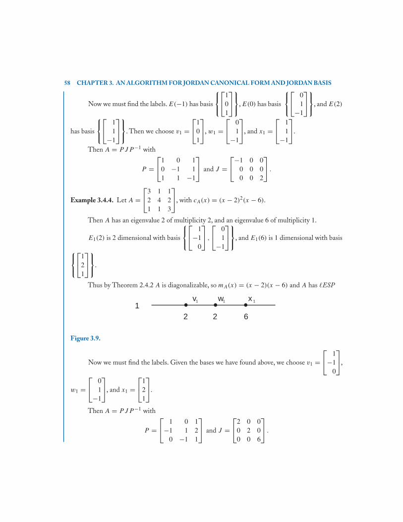
58 CHAPTER 3. AN ALGORITHM FOR JORDAN CANONICAL FORM AND JORDAN BASIS
Now we must find the labels. E(−1) has basis
⎧⎨⎩
⎡⎣1
01
⎤⎦
⎫⎬⎭, E(0) has basis
⎧⎨⎩
⎡⎣ 0
1−1
⎤⎦
⎫⎬⎭, and E(2)
has basis
⎧⎨⎩
⎡⎣ 1
1−1
⎤⎦
⎫⎬⎭. Then we choose v1 =
⎡⎣1
01
⎤⎦, w1 =
⎡⎣ 0
1−1
⎤⎦, and x1 =
⎡⎣ 1
1−1
⎤⎦.
Then A = PJP −1 with
P =⎡⎣1 0 1
0 −1 11 1 −1
⎤⎦ and J =
⎡⎣−1 0 0
0 0 00 0 2
⎤⎦ .
Example 3.4.4. Let A =⎡⎣3 1 1
2 4 21 1 3
⎤⎦, with cA(x) = (x − 2)2(x − 6).
Then A has an eigenvalue 2 of multiplicity 2, and an eigenvalue 6 of multiplicity 1.
E1(2) is 2 dimensional with basis
⎧⎨⎩
⎡⎣ 1
−10
⎤⎦ ,
⎡⎣ 0
1−1
⎤⎦
⎫⎬⎭, and E1(6) is 1 dimensional with basis
⎧⎨⎩
⎡⎣1
21
⎤⎦
⎫⎬⎭.
Thus by Theorem 2.4.2 A is diagonalizable, so mA(x) = (x − 2)(x − 6) and A has �ESP
2 2 61
v1 w1 x 1
Figure 3.9.
Now we must find the labels. Given the bases we have found above, we choose v1 =⎡⎣ 1
−10
⎤⎦,
w1 =⎡⎣ 0
1−1
⎤⎦, and x1 =
⎡⎣1
21
⎤⎦.
Then A = PJP −1 with
P =⎡⎣ 1 0 1
−1 1 20 −1 1
⎤⎦ and J =
⎡⎣2 0 0
0 2 00 0 6
⎤⎦ .

3.4. EXAMPLES 59
Example 3.4.5. Let A =⎡⎣ 2 1 1
2 1 −2−1 0 −2
⎤⎦, with cA(x) = (x + 1)2(x − 3).
Then A has an eigenvalue −1 of multiplicity 2, and an eigenvalue 3 of multiplicity 1.
E1(−1) is 1 dimensional with basis
⎧⎨⎩
⎡⎣ 1
−21
⎤⎦
⎫⎬⎭, and E2(−1) is 2 dimensional with basis
⎧⎨⎩
⎡⎣ 1
−20
⎤⎦ ,
⎡⎣0
01
⎤⎦
⎫⎬⎭. E1(3) is 1 dimensional with basis
⎧⎨⎩
⎡⎣ 5
6−1
⎤⎦
⎫⎬⎭.
Thus d1(−1) = 1, d2(−1) = 2, so dex2 (−1) = 1, dex
1 (−1) = 1, and dnew2 (−1) = 1,
dnew1 (−1) = 0. Also d1(3) = dex
1 (3) = dnew1 (3) = 1.
Thus mA(x) = (x + 1)2(x − 3) and A has �ESP
-11
2 v2
v1 w1
3
Figure 3.10.
Now we must find the labels. We must choose v2 to be a vector that is in E2(−1) but
that is not in E1(−1). Given the bases we have found above, we choose v2 =⎡⎣ 1
−20
⎤⎦, and then
v1 = (A − (−1)I )v2 =⎡⎣ 1
−21
⎤⎦. (It is purely a coincidence that v1 was a vector in the basis we chose
for E1(−1), and that will in general not be the case. Compare Example 3.4.2, where it wasn’t.) Also,
we choose w1 =⎡⎣ 5
6−1
⎤⎦.
Then A = PJP −1 with
P =⎡⎣ 1 1 5
−2 −2 61 0 −1
⎤⎦ and J =
⎡⎣−1 1 0
0 −1 00 0 3
⎤⎦ .
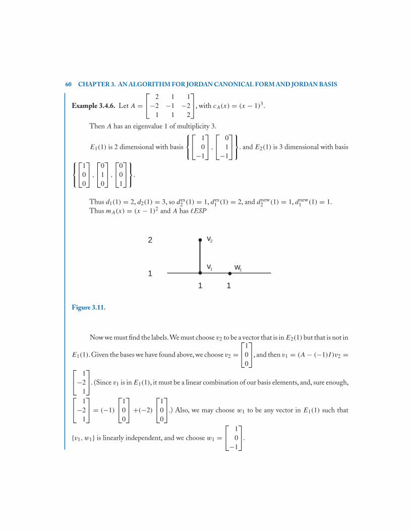
60 CHAPTER 3. AN ALGORITHM FOR JORDAN CANONICAL FORM AND JORDAN BASIS
Example 3.4.6. Let A =⎡⎣ 2 1 1
−2 −1 −21 1 2
⎤⎦, with cA(x) = (x − 1)3.
Then A has an eigenvalue 1 of multiplicity 3.
E1(1) is 2 dimensional with basis
⎧⎨⎩
⎡⎣ 1
0−1
⎤⎦ ,
⎡⎣ 0
1−1
⎤⎦
⎫⎬⎭. and E2(1) is 3 dimensional with basis
⎧⎨⎩
⎡⎣1
00
⎤⎦ ,
⎡⎣0
10
⎤⎦ ,
⎡⎣0
01
⎤⎦
⎫⎬⎭.
Thus d1(1) = 2, d2(1) = 3, so dex2 (1) = 1, dex
1 (1) = 2, and dnew2 (1) = 1, dnew
1 (1) = 1.Thus mA(x) = (x − 1)2 and A has �ESP
1 11
2 v2
v1 w1
Figure 3.11.
Now we must find the labels.We must choose v2 to be a vector that is in E2(1) but that is not in
E1(1). Given the bases we have found above, we choose v2 =⎡⎣1
00
⎤⎦, and then v1 = (A − (−1)I )v2 =
⎡⎣ 1
−21
⎤⎦. (Since v1 is in E1(1), it must be a linear combination of our basis elements, and, sure enough,
⎡⎣ 1
−21
⎤⎦ = (−1)
⎡⎣1
00
⎤⎦ +(−2)
⎡⎣1
00
⎤⎦.) Also, we may choose w1 to be any vector in E1(1) such that
{v1, w1} is linearly independent, and we choose w1 =⎡⎣ 1
0−1
⎤⎦.
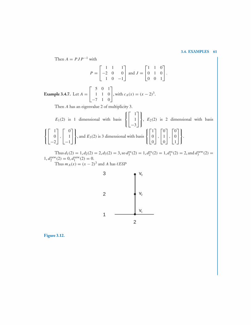
3.4. EXAMPLES 61
Then A = PJP −1 with
P =⎡⎣ 1 1 1
−2 0 01 0 −1
⎤⎦ and J =
⎡⎣1 1 0
0 1 00 0 1
⎤⎦ .
Example 3.4.7. Let A =⎡⎣ 5 0 1
1 1 0−7 1 0
⎤⎦, with cA(x) = (x − 2)3.
Then A has an eigenvalue 2 of multiplicity 3.
E1(2) is 1 dimensional with basis
⎧⎨⎩
⎡⎣ 1
1−3
⎤⎦
⎫⎬⎭, E2(2) is 2 dimensional with basis
⎧⎨⎩
⎡⎣ 1
0−2
⎤⎦ ,
⎡⎣ 0
1−1
⎤⎦
⎫⎬⎭, and E3(2) is 3 dimensional with basis
⎧⎨⎩
⎡⎣1
00
⎤⎦ ,
⎡⎣0
10
⎤⎦ ,
⎡⎣0
01
⎤⎦
⎫⎬⎭.
Thus d1(2) = 1, d2(2) = 2, d3(2) = 3, so dex3 (2) = 1, dex
2 (2) = 1, dex1 (2) = 2, and dnew
3 (2) =1, dnew
2 (2) = 0, dnew1 (2) = 0.
Thus mA(x) = (x − 2)3 and A has �ESP
21
2
3
v2
v3
v1
Figure 3.12.

62 CHAPTER 3. AN ALGORITHM FOR JORDAN CANONICAL FORM AND JORDAN BASIS
Now we must find the labels. We must choose v3 to be a vector that is in E2(3) but that is
not in E2(3). Given the bases we have found above, we choose v3 =⎡⎣1
00
⎤⎦, then v2 = (A − 2I )v2 =
⎡⎣ 3
1−7
⎤⎦, and v1 = (A − 2)I )v2 =
⎡⎣ 2
2−6
⎤⎦.
Then A = PJP −1 with
P =⎡⎣ 2 3 1
2 1 0−6 −7 0
⎤⎦ and J =
⎡⎣2 1 0
0 2 10 0 2
⎤⎦ .
Example 3.4.8. Let A =
⎡⎢⎢⎣
0 1 1 −112 6 −6 6
6 2 −1 316 0 −8 10
⎤⎥⎥⎦, with cA(x) = (x − 2)3(x − 5).
Then A has an eigenvalue 2 of multiplicity 3, and an eigenvalue 5 of multiplicity 1.
E1(2) is 2 dimensional with basis
⎧⎪⎪⎨⎪⎪⎩
⎡⎢⎢⎣
1020
⎤⎥⎥⎦ ,
⎡⎢⎢⎣
0011
⎤⎥⎥⎦
⎫⎪⎪⎬⎪⎪⎭
, and E2(2) is 3 dimensional with basis
⎧⎪⎪⎨⎪⎪⎩
⎡⎢⎢⎣
1020
⎤⎥⎥⎦ ,
⎡⎢⎢⎣
0100
⎤⎥⎥⎦ ,
⎡⎢⎢⎣
0011
⎤⎥⎥⎦
⎫⎪⎪⎬⎪⎪⎭
. E1(5) is 1 dimensional with basis
⎧⎪⎪⎨⎪⎪⎩
⎡⎢⎢⎣
1678
⎤⎥⎥⎦
⎫⎪⎪⎬⎪⎪⎭
,
Thus d1(2) = 2, d2(2) = 3, so dex2 (2) = 1, dex
1 (2) = 2, and dnew2 (2) = 1, dnew
1 (2) = 1. Also,d1(5) = dex
1 (5) = dnew1 (2) = 5.
Thus mA(x) = (x − 1)2(x − 5) and A has �ESP
2
21
2
2 5
1 1 1
V
V W x
Figure 3.13.
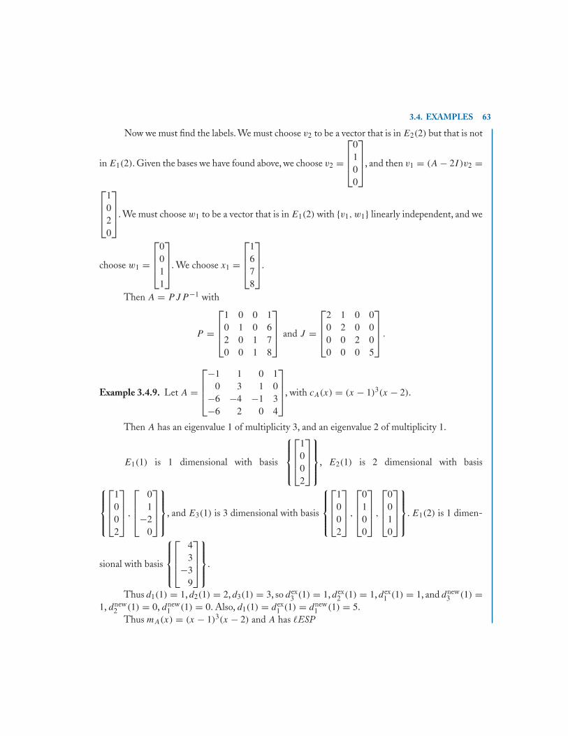
3.4. EXAMPLES 63
Now we must find the labels. We must choose v2 to be a vector that is in E2(2) but that is not
in E1(2). Given the bases we have found above, we choose v2 =
⎡⎢⎢⎣
0100
⎤⎥⎥⎦, and then v1 = (A − 2I )v2 =
⎡⎢⎢⎣
1020
⎤⎥⎥⎦. We must choose w1 to be a vector that is in E1(2) with {v1, w1} linearly independent, and we
choose w1 =
⎡⎢⎢⎣
0011
⎤⎥⎥⎦. We choose x1 =
⎡⎢⎢⎣
1678
⎤⎥⎥⎦.
Then A = PJP −1 with
P =
⎡⎢⎢⎣
1 0 0 10 1 0 62 0 1 70 0 1 8
⎤⎥⎥⎦ and J =
⎡⎢⎢⎣
2 1 0 00 2 0 00 0 2 00 0 0 5
⎤⎥⎥⎦ .
Example 3.4.9. Let A =
⎡⎢⎢⎣
−1 1 0 10 3 1 0
−6 −4 −1 3−6 2 0 4
⎤⎥⎥⎦, with cA(x) = (x − 1)3(x − 2).
Then A has an eigenvalue 1 of multiplicity 3, and an eigenvalue 2 of multiplicity 1.
E1(1) is 1 dimensional with basis
⎧⎪⎪⎨⎪⎪⎩
⎡⎢⎢⎣
1002
⎤⎥⎥⎦
⎫⎪⎪⎬⎪⎪⎭
, E2(1) is 2 dimensional with basis
⎧⎪⎪⎨⎪⎪⎩
⎡⎢⎢⎣
1002
⎤⎥⎥⎦ ,
⎡⎢⎢⎣
01
−20
⎤⎥⎥⎦
⎫⎪⎪⎬⎪⎪⎭
, and E3(1) is 3 dimensional with basis
⎧⎪⎪⎨⎪⎪⎩
⎡⎢⎢⎣
1002
⎤⎥⎥⎦ ,
⎡⎢⎢⎣
0100
⎤⎥⎥⎦ ,
⎡⎢⎢⎣
0010
⎤⎥⎥⎦
⎫⎪⎪⎬⎪⎪⎭
. E1(2) is 1 dimen-
sional with basis
⎧⎪⎪⎨⎪⎪⎩
⎡⎢⎢⎣
43
−39
⎤⎥⎥⎦
⎫⎪⎪⎬⎪⎪⎭
.
Thus d1(1) = 1, d2(1) = 2, d3(1) = 3, so dex3 (1) = 1, dex
2 (1) = 1, dex1 (1) = 1, and dnew
3 (1) =1, dnew
2 (1) = 0, dnew1 (1) = 0. Also, d1(1) = dex
1 (1) = dnew1 (1) = 5.
Thus mA(x) = (x − 1)3(x − 2) and A has �ESP

64 CHAPTER 3. AN ALGORITHM FOR JORDAN CANONICAL FORM AND JORDAN BASIS
V2
3
11
2
3
1 1V
V
W
2
Figure 3.14.
Now we must find the labels. We must choose v3 to be a vector that is in E3(1) but that isnot in E2(1).
Given the bases we have found above, we choose v3 =
⎡⎢⎢⎣
0100
⎤⎥⎥⎦, then v2 = (A − 1I )v3 =
⎡⎢⎢⎣
12
−42
⎤⎥⎥⎦, and
then v1 = (A − 1I )v2 =
⎡⎢⎢⎣
2004
⎤⎥⎥⎦. Also, we choose w1 =
⎡⎢⎢⎣
43
−39
⎤⎥⎥⎦.
Then A = PJP −1 with
P =
⎡⎢⎢⎣
2 1 0 40 2 1 30 −4 0 −34 2 0 9
⎤⎥⎥⎦ and J =
⎡⎢⎢⎣
1 1 0 00 1 1 00 0 1 00 0 0 2
⎤⎥⎥⎦ .
Example 3.4.10. Let A =
⎡⎢⎢⎣
4 1 −1 2−2 7 −2 4
3 −3 8 −62 −2 2 1
⎤⎥⎥⎦, with cA(x) = (x − 5)4.
Then A has an eigenvalue 5 of multiplicity 4.
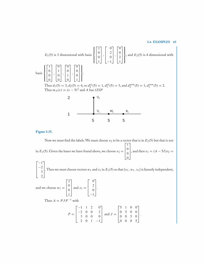
3.4. EXAMPLES 65
E1(5) is 3 dimensional with basis
⎧⎪⎪⎨⎪⎪⎩
⎡⎢⎢⎣
2001
⎤⎥⎥⎦ ,
⎡⎢⎢⎣
020
−1
⎤⎥⎥⎦ ,
⎡⎢⎢⎣
0021
⎤⎥⎥⎦
⎫⎪⎪⎬⎪⎪⎭
, and E2(5) is 4 dimensional with
basis
⎧⎪⎪⎨⎪⎪⎩
⎡⎢⎢⎣
1000
⎤⎥⎥⎦ ,
⎡⎢⎢⎣
0100
⎤⎥⎥⎦ ,
⎡⎢⎢⎣
0010
⎤⎥⎥⎦ ,
⎡⎢⎢⎣
0001
⎤⎥⎥⎦
⎫⎪⎪⎬⎪⎪⎭
.
Thus d1(5) = 3, d2(5) = 4, so dex2 (5) = 1, dex
1 (5) = 3, and dnew2 (5) = 1, dnew
1 (5) = 2.Thus mA(x) = (x − 5)2 and A has �ESP
2
15 5 5
2
1 1 1
V
V W x
Figure 3.15.
Now we must find the labels. We must choose v2 to be a vector that is in E2(5) but that is not
in E1(5). Given the bases we have found above, we choose v2 =
⎡⎢⎢⎣
1000
⎤⎥⎥⎦, and then v1 = (A − 5I )v2 =
⎡⎢⎢⎣
−1−2
32
⎤⎥⎥⎦.Then we must choose vectors w1 and x1 in E1(5) so that {v1, w1, x1} is linearly independent,
and we choose w1 =
⎡⎢⎢⎣
2001
⎤⎥⎥⎦ and x1 =
⎡⎢⎢⎣
020
−1
⎤⎥⎥⎦.
Then A = PJP −1 with
P =
⎡⎢⎢⎣
−1 1 2 0−2 0 0 2
3 0 0 02 0 1 −1
⎤⎥⎥⎦ and J =
⎡⎢⎢⎣
5 1 0 00 5 0 00 0 5 00 0 0 5
⎤⎥⎥⎦ .

66 CHAPTER 3. AN ALGORITHM FOR JORDAN CANONICAL FORM AND JORDAN BASIS
Example 3.4.11. Let A =
⎡⎢⎢⎣
7 −2 −1 31 3 0 11 −1 4 1
−2 1 1 2
⎤⎥⎥⎦, with cA(x) = (x − 4)4.
Then A has an eigenvalue 4 of multiplicity 4.
E1(4) is 2 dimensional with basis
⎧⎪⎪⎨⎪⎪⎩
⎡⎢⎢⎣
1110
⎤⎥⎥⎦ ,
⎡⎢⎢⎣
0111
⎤⎥⎥⎦
⎫⎪⎪⎬⎪⎪⎭
= {t1, u1}, and E2(4) is 4 dimensional with
basis
⎧⎪⎪⎨⎪⎪⎩
⎡⎢⎢⎣
1000
⎤⎥⎥⎦ ,
⎡⎢⎢⎣
0100
⎤⎥⎥⎦ ,
⎡⎢⎢⎣
0010
⎤⎥⎥⎦ ,
⎡⎢⎢⎣
0001
⎤⎥⎥⎦
⎫⎪⎪⎬⎪⎪⎭
.
Thus d1(4) = 2, d2(4) = 4, so dex2 (4) = 2, dex
1 (4) = 2, and dnew2 (4) = 2, dnew
1 (4) = 0.Thus mA(x) = (x − 4)4 and A has �ESP
v2
v
441
2
1 w1
w2
Figure 3.16.
Now we must find the labels. We must choose v2 and w2 to be vectors in E2(4) with
{v2, w2, t1, u1} linearly independent. Given the bases we have found above, we choose v2 =
⎡⎢⎢⎣
1000
⎤⎥⎥⎦
and w2 =
⎡⎢⎢⎣
0100
⎤⎥⎥⎦. Then v1 = (A − 4I )v2 =
⎡⎢⎢⎣
311
−2
⎤⎥⎥⎦ and w1 =
⎡⎢⎢⎣
−2−1−1
1
⎤⎥⎥⎦.
Then A = PJP −1 with
P =
⎡⎢⎢⎣
3 1 −2 01 0 −1 11 0 −1 0
−2 0 1 0
⎤⎥⎥⎦ and J =
⎡⎢⎢⎣
4 1 0 00 4 0 00 0 4 10 0 0 4
⎤⎥⎥⎦ .

3.4. EXAMPLES 67
Example 3.4.12. Let A =
⎡⎢⎢⎢⎢⎢⎢⎢⎣
−2 −7 −10 5 8 5−1 1 −1 1 2 1−1 −3 1 1 3 1−4 −7 −8 7 7 4−2 −1 −3 2 4 2−2 −6 −4 2 7 5
⎤⎥⎥⎥⎥⎥⎥⎥⎦
, with cA(x) = (x − 3)4(x − 2)2.
Then A has an eigenvalue 3 of multiplicity 4, and an eigenvalue 2 of multiplicity 2.
E1(3) is 2 dimensional with basis
⎧⎪⎪⎪⎪⎪⎪⎪⎨⎪⎪⎪⎪⎪⎪⎪⎩
⎡⎢⎢⎢⎢⎢⎢⎢⎣
100001
⎤⎥⎥⎥⎥⎥⎥⎥⎦
,
⎡⎢⎢⎢⎢⎢⎢⎢⎣
00010
−1
⎤⎥⎥⎥⎥⎥⎥⎥⎦
⎫⎪⎪⎪⎪⎪⎪⎪⎬⎪⎪⎪⎪⎪⎪⎪⎭
, E2(3) is 3 dimensional with basis
⎧⎪⎪⎪⎪⎪⎪⎪⎨⎪⎪⎪⎪⎪⎪⎪⎩
⎡⎢⎢⎢⎢⎢⎢⎢⎣
100001
⎤⎥⎥⎥⎥⎥⎥⎥⎦
,
⎡⎢⎢⎢⎢⎢⎢⎢⎣
010010
⎤⎥⎥⎥⎥⎥⎥⎥⎦
,
⎡⎢⎢⎢⎢⎢⎢⎢⎣
00010
−1
⎤⎥⎥⎥⎥⎥⎥⎥⎦
⎫⎪⎪⎪⎪⎪⎪⎪⎬⎪⎪⎪⎪⎪⎪⎪⎭
, and E3(3) is 4 dimensional with basis
⎧⎪⎪⎪⎪⎪⎪⎪⎨⎪⎪⎪⎪⎪⎪⎪⎩
⎡⎢⎢⎢⎢⎢⎢⎢⎣
100001
⎤⎥⎥⎥⎥⎥⎥⎥⎦
,
⎡⎢⎢⎢⎢⎢⎢⎢⎣
010010
⎤⎥⎥⎥⎥⎥⎥⎥⎦
,
⎡⎢⎢⎢⎢⎢⎢⎢⎣
001002
⎤⎥⎥⎥⎥⎥⎥⎥⎦
,
⎡⎢⎢⎢⎢⎢⎢⎢⎣
00010
−1
⎤⎥⎥⎥⎥⎥⎥⎥⎦
⎫⎪⎪⎪⎪⎪⎪⎪⎬⎪⎪⎪⎪⎪⎪⎪⎭
.
Also, E1(2) is 1 dimensional with basis
⎧⎪⎪⎪⎪⎪⎪⎪⎨⎪⎪⎪⎪⎪⎪⎪⎩
⎡⎢⎢⎢⎢⎢⎢⎢⎣
9−1
37
−28
⎤⎥⎥⎥⎥⎥⎥⎥⎦
⎫⎪⎪⎪⎪⎪⎪⎪⎬⎪⎪⎪⎪⎪⎪⎪⎭
, and E2(2) is 2 dimensional with basis
⎧⎪⎪⎪⎪⎪⎪⎪⎨⎪⎪⎪⎪⎪⎪⎪⎩
⎡⎢⎢⎢⎢⎢⎢⎢⎣
−180
−8−17
4−18
⎤⎥⎥⎥⎥⎥⎥⎥⎦
,
⎡⎢⎢⎢⎢⎢⎢⎢⎣
022302
⎤⎥⎥⎥⎥⎥⎥⎥⎦
⎫⎪⎪⎪⎪⎪⎪⎪⎬⎪⎪⎪⎪⎪⎪⎪⎭
.
Thus d1(3) = 2, d2(3) = 3, d3(3) = 4, so dex3 (3) = 1, dex
2 (3) = 1, dex1 (3) = 2, and dnew
3 (3) =1, dnew
2 (3) = 0, dnew1 (3) = 1. Also, d1(2) = 1, d2(2) = 2, so dex
2 (2) = 1, dex1 (2) = 1, and dnew
2 (2) =1, dnew
1 (2) = 0.Thus mA(x) = (x − 3)3(x − 2)2 and A has �ESP
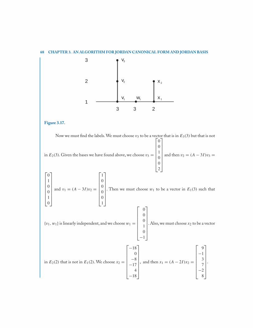
68 CHAPTER 3. AN ALGORITHM FOR JORDAN CANONICAL FORM AND JORDAN BASIS
v2
v3
v
3 231
2
3
1 w1 x 1
x 2
Figure 3.17.
Now we must find the labels. We must choose v3 to be a vector that is in E3(3) but that is not
in E2(3). Given the bases we have found above, we choose v3 =
⎡⎢⎢⎢⎢⎢⎢⎢⎣
001002
⎤⎥⎥⎥⎥⎥⎥⎥⎦
and then v2 = (A − 3I )v3 =
⎡⎢⎢⎢⎢⎢⎢⎢⎣
010010
⎤⎥⎥⎥⎥⎥⎥⎥⎦
and v1 = (A − 3I )v2 =
⎡⎢⎢⎢⎢⎢⎢⎢⎣
100001
⎤⎥⎥⎥⎥⎥⎥⎥⎦
. Then we must choose w1 to be a vector in E1(3) such that
{v1, w1} is linearly independent, and we choose w1 =
⎡⎢⎢⎢⎢⎢⎢⎢⎣
00010
−1
⎤⎥⎥⎥⎥⎥⎥⎥⎦
. Also, we must choose x2 to be a vector
in E2(2) that is not in E1(2). We choose x2 =
⎡⎢⎢⎢⎢⎢⎢⎢⎣
−180
−8−17
4−18
⎤⎥⎥⎥⎥⎥⎥⎥⎦
, and then x1 = (A − 2I )x2 =
⎡⎢⎢⎢⎢⎢⎢⎢⎣
9−1
37
−28
⎤⎥⎥⎥⎥⎥⎥⎥⎦
.
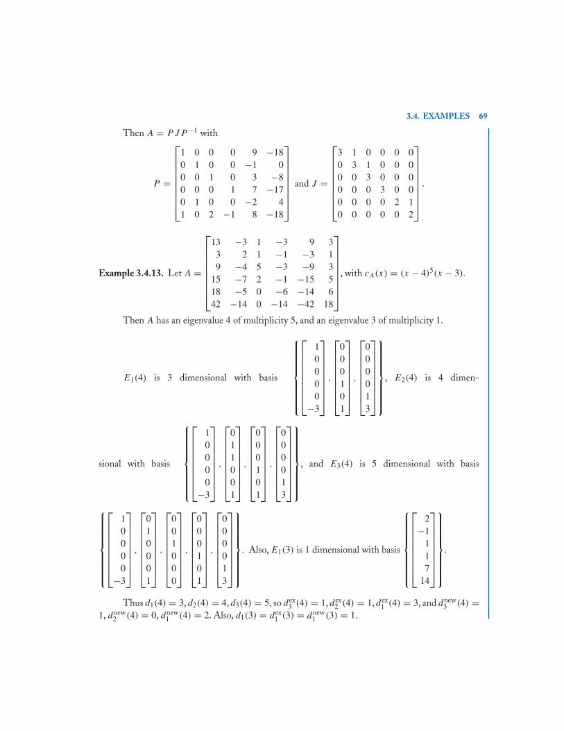
3.4. EXAMPLES 69
Then A = PJP −1 with
P =
⎡⎢⎢⎢⎢⎢⎢⎢⎣
1 0 0 0 9 −180 1 0 0 −1 00 0 1 0 3 −80 0 0 1 7 −170 1 0 0 −2 41 0 2 −1 8 −18
⎤⎥⎥⎥⎥⎥⎥⎥⎦
and J =
⎡⎢⎢⎢⎢⎢⎢⎢⎣
3 1 0 0 0 00 3 1 0 0 00 0 3 0 0 00 0 0 3 0 00 0 0 0 2 10 0 0 0 0 2
⎤⎥⎥⎥⎥⎥⎥⎥⎦
.
Example 3.4.13. Let A =
⎡⎢⎢⎢⎢⎢⎢⎢⎣
13 −3 1 −3 9 33 2 1 −1 −3 19 −4 5 −3 −9 3
15 −7 2 −1 −15 518 −5 0 −6 −14 642 −14 0 −14 −42 18
⎤⎥⎥⎥⎥⎥⎥⎥⎦
, with cA(x) = (x − 4)5(x − 3).
Then A has an eigenvalue 4 of multiplicity 5, and an eigenvalue 3 of multiplicity 1.
E1(4) is 3 dimensional with basis
⎧⎪⎪⎪⎪⎪⎪⎪⎨⎪⎪⎪⎪⎪⎪⎪⎩
⎡⎢⎢⎢⎢⎢⎢⎢⎣
10000
−3
⎤⎥⎥⎥⎥⎥⎥⎥⎦
,
⎡⎢⎢⎢⎢⎢⎢⎢⎣
000101
⎤⎥⎥⎥⎥⎥⎥⎥⎦
,
⎡⎢⎢⎢⎢⎢⎢⎢⎣
000013
⎤⎥⎥⎥⎥⎥⎥⎥⎦
⎫⎪⎪⎪⎪⎪⎪⎪⎬⎪⎪⎪⎪⎪⎪⎪⎭
, E2(4) is 4 dimen-
sional with basis
⎧⎪⎪⎪⎪⎪⎪⎪⎨⎪⎪⎪⎪⎪⎪⎪⎩
⎡⎢⎢⎢⎢⎢⎢⎢⎣
10000
−3
⎤⎥⎥⎥⎥⎥⎥⎥⎦
,
⎡⎢⎢⎢⎢⎢⎢⎢⎣
011001
⎤⎥⎥⎥⎥⎥⎥⎥⎦
,
⎡⎢⎢⎢⎢⎢⎢⎢⎣
000101
⎤⎥⎥⎥⎥⎥⎥⎥⎦
,
⎡⎢⎢⎢⎢⎢⎢⎢⎣
000013
⎤⎥⎥⎥⎥⎥⎥⎥⎦
⎫⎪⎪⎪⎪⎪⎪⎪⎬⎪⎪⎪⎪⎪⎪⎪⎭
, and E3(4) is 5 dimensional with basis
⎧⎪⎪⎪⎪⎪⎪⎪⎨⎪⎪⎪⎪⎪⎪⎪⎩
⎡⎢⎢⎢⎢⎢⎢⎢⎣
10000
−3
⎤⎥⎥⎥⎥⎥⎥⎥⎦
,
⎡⎢⎢⎢⎢⎢⎢⎢⎣
010001
⎤⎥⎥⎥⎥⎥⎥⎥⎦
,
⎡⎢⎢⎢⎢⎢⎢⎢⎣
001000
⎤⎥⎥⎥⎥⎥⎥⎥⎦
,
⎡⎢⎢⎢⎢⎢⎢⎢⎣
000101
⎤⎥⎥⎥⎥⎥⎥⎥⎦
,
⎡⎢⎢⎢⎢⎢⎢⎢⎣
000013
⎤⎥⎥⎥⎥⎥⎥⎥⎦
⎫⎪⎪⎪⎪⎪⎪⎪⎬⎪⎪⎪⎪⎪⎪⎪⎭
. Also, E1(3) is 1 dimensional with basis
⎧⎪⎪⎪⎪⎪⎪⎪⎨⎪⎪⎪⎪⎪⎪⎪⎩
⎡⎢⎢⎢⎢⎢⎢⎢⎣
2−1
117
14
⎤⎥⎥⎥⎥⎥⎥⎥⎦
⎫⎪⎪⎪⎪⎪⎪⎪⎬⎪⎪⎪⎪⎪⎪⎪⎭
.
Thus d1(4) = 3, d2(4) = 4, d3(4) = 5, so dex3 (4) = 1, dex
2 (4) = 1, dex1 (4) = 3, and dnew
3 (4) =1, dnew
2 (4) = 0, dnew1 (4) = 2. Also, d1(3) = dex
1 (3) = dnew1 (3) = 1.
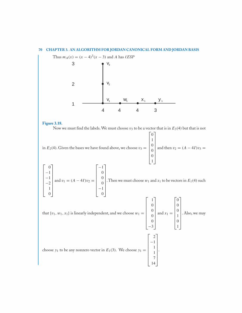
70 CHAPTER 3. AN ALGORITHM FOR JORDAN CANONICAL FORM AND JORDAN BASIS
Thus mA(x) = (x − 4)3(x − 3) and A has �ESP
v2
v3
v
4 4 341
2
3
1 w1 x 1 y 1
Figure 3.18.Now we must find the labels. We must choose v3 to be a vector that is in E3(4) but that is not
in E2(4). Given the bases we have found above, we choose v3 =
⎡⎢⎢⎢⎢⎢⎢⎢⎣
010001
⎤⎥⎥⎥⎥⎥⎥⎥⎦
and then v2 = (A − 4I )v3 =
⎡⎢⎢⎢⎢⎢⎢⎢⎣
0−1−1−2
10
⎤⎥⎥⎥⎥⎥⎥⎥⎦
and v1 = (A − 4I )v2 =
⎡⎢⎢⎢⎢⎢⎢⎢⎣
−1000
−10
⎤⎥⎥⎥⎥⎥⎥⎥⎦
.Then we must choose w1 and x1 to be vectors in E1(4) such
that {v1, w1, x1} is linearly independent, and we choose w1 =
⎡⎢⎢⎢⎢⎢⎢⎢⎣
10000
−3
⎤⎥⎥⎥⎥⎥⎥⎥⎦
and x1 =
⎡⎢⎢⎢⎢⎢⎢⎢⎣
000101
⎤⎥⎥⎥⎥⎥⎥⎥⎦
. Also, we may
choose y1 to be any nonzero vector in E1(3). We choose y1 =
⎡⎢⎢⎢⎢⎢⎢⎢⎣
2−1
117
14
⎤⎥⎥⎥⎥⎥⎥⎥⎦
.
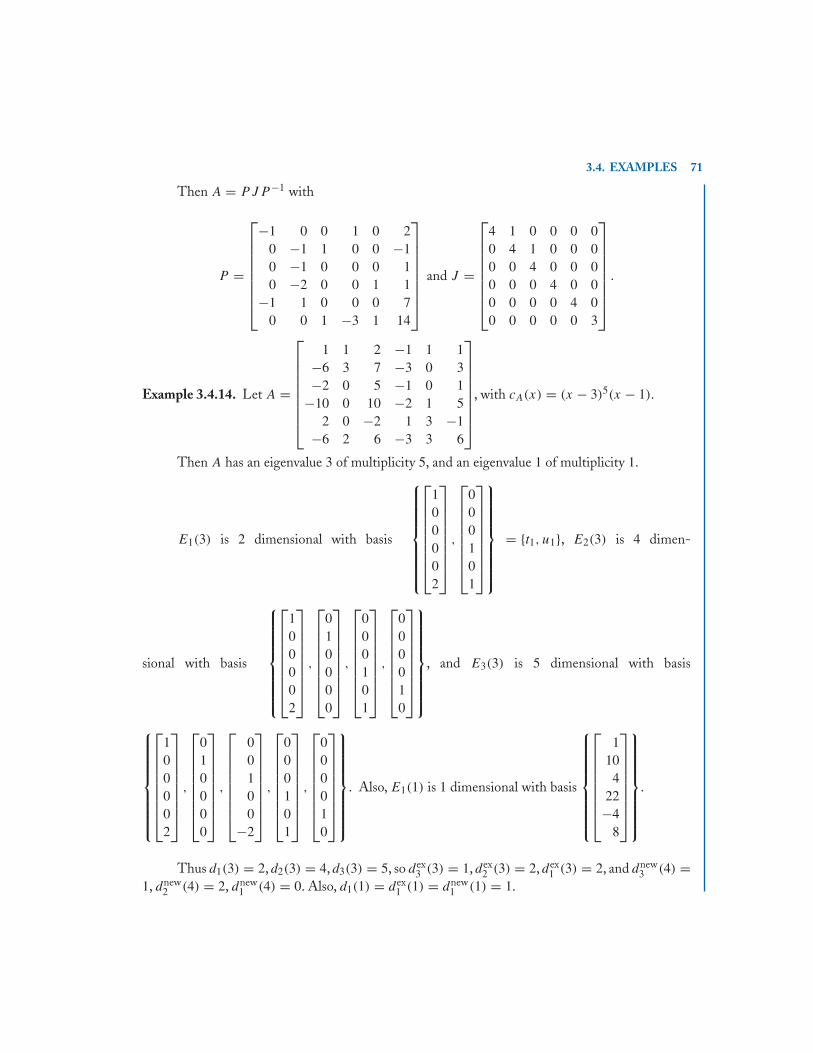
3.4. EXAMPLES 71
Then A = PJP −1 with
P =
⎡⎢⎢⎢⎢⎢⎢⎢⎣
−1 0 0 1 0 20 −1 1 0 0 −10 −1 0 0 0 10 −2 0 0 1 1
−1 1 0 0 0 70 0 1 −3 1 14
⎤⎥⎥⎥⎥⎥⎥⎥⎦
and J =
⎡⎢⎢⎢⎢⎢⎢⎢⎣
4 1 0 0 0 00 4 1 0 0 00 0 4 0 0 00 0 0 4 0 00 0 0 0 4 00 0 0 0 0 3
⎤⎥⎥⎥⎥⎥⎥⎥⎦
.
Example 3.4.14. Let A =
⎡⎢⎢⎢⎢⎢⎢⎢⎣
1 1 2 −1 1 1−6 3 7 −3 0 3−2 0 5 −1 0 1
−10 0 10 −2 1 52 0 −2 1 3 −1
−6 2 6 −3 3 6
⎤⎥⎥⎥⎥⎥⎥⎥⎦
, with cA(x) = (x − 3)5(x − 1).
Then A has an eigenvalue 3 of multiplicity 5, and an eigenvalue 1 of multiplicity 1.
E1(3) is 2 dimensional with basis
⎧⎪⎪⎪⎪⎪⎪⎪⎨⎪⎪⎪⎪⎪⎪⎪⎩
⎡⎢⎢⎢⎢⎢⎢⎢⎣
100002
⎤⎥⎥⎥⎥⎥⎥⎥⎦
,
⎡⎢⎢⎢⎢⎢⎢⎢⎣
000101
⎤⎥⎥⎥⎥⎥⎥⎥⎦
⎫⎪⎪⎪⎪⎪⎪⎪⎬⎪⎪⎪⎪⎪⎪⎪⎭
= {t1, u1}, E2(3) is 4 dimen-
sional with basis
⎧⎪⎪⎪⎪⎪⎪⎪⎨⎪⎪⎪⎪⎪⎪⎪⎩
⎡⎢⎢⎢⎢⎢⎢⎢⎣
100002
⎤⎥⎥⎥⎥⎥⎥⎥⎦
,
⎡⎢⎢⎢⎢⎢⎢⎢⎣
010000
⎤⎥⎥⎥⎥⎥⎥⎥⎦
,
⎡⎢⎢⎢⎢⎢⎢⎢⎣
000101
⎤⎥⎥⎥⎥⎥⎥⎥⎦
,
⎡⎢⎢⎢⎢⎢⎢⎢⎣
000010
⎤⎥⎥⎥⎥⎥⎥⎥⎦
⎫⎪⎪⎪⎪⎪⎪⎪⎬⎪⎪⎪⎪⎪⎪⎪⎭
, and E3(3) is 5 dimensional with basis
⎧⎪⎪⎪⎪⎪⎪⎪⎨⎪⎪⎪⎪⎪⎪⎪⎩
⎡⎢⎢⎢⎢⎢⎢⎢⎣
100002
⎤⎥⎥⎥⎥⎥⎥⎥⎦
,
⎡⎢⎢⎢⎢⎢⎢⎢⎣
010000
⎤⎥⎥⎥⎥⎥⎥⎥⎦
,
⎡⎢⎢⎢⎢⎢⎢⎢⎣
00100
−2
⎤⎥⎥⎥⎥⎥⎥⎥⎦
,
⎡⎢⎢⎢⎢⎢⎢⎢⎣
000101
⎤⎥⎥⎥⎥⎥⎥⎥⎦
,
⎡⎢⎢⎢⎢⎢⎢⎢⎣
000010
⎤⎥⎥⎥⎥⎥⎥⎥⎦
⎫⎪⎪⎪⎪⎪⎪⎪⎬⎪⎪⎪⎪⎪⎪⎪⎭
. Also, E1(1) is 1 dimensional with basis
⎧⎪⎪⎪⎪⎪⎪⎪⎨⎪⎪⎪⎪⎪⎪⎪⎩
⎡⎢⎢⎢⎢⎢⎢⎢⎣
110
422−4
8
⎤⎥⎥⎥⎥⎥⎥⎥⎦
⎫⎪⎪⎪⎪⎪⎪⎪⎬⎪⎪⎪⎪⎪⎪⎪⎭
.
Thus d1(3) = 2, d2(3) = 4, d3(3) = 5, so dex3 (3) = 1, dex
2 (3) = 2, dex1 (3) = 2, and dnew
3 (4) =1, dnew
2 (4) = 2, dnew1 (4) = 0. Also, d1(1) = dex
1 (1) = dnew1 (1) = 1.

72 CHAPTER 3. AN ALGORITHM FOR JORDAN CANONICAL FORM AND JORDAN BASIS
Thus mA(x) = (x − 3)3(x − 1) and A has �ESP
3
2
1
v3
v2
v
3 3
1
w2
w1 x1
1
Figure 3.19.
Now we must find the labels. We must choose v3 to be a vector that is in E3(4) but that is not
in E2(4). Given the bases we have found above, we choose v3 =
⎡⎢⎢⎢⎢⎢⎢⎢⎣
01000
−2
⎤⎥⎥⎥⎥⎥⎥⎥⎦
and then v2 = (A − 4I )v3 =
⎡⎢⎢⎢⎢⎢⎢⎢⎣
010000
⎤⎥⎥⎥⎥⎥⎥⎥⎦
. Now we must choose w2 in E2(3) so that {v2, w2, t1, u1} is linearly independent. We choose
w2 =
⎡⎢⎢⎢⎢⎢⎢⎢⎣
000010
⎤⎥⎥⎥⎥⎥⎥⎥⎦
. Then v1 = (A − 3I )v2 =
⎡⎢⎢⎢⎢⎢⎢⎢⎣
100002
⎤⎥⎥⎥⎥⎥⎥⎥⎦
and w1 = (A − 3I )w2 =
⎡⎢⎢⎢⎢⎢⎢⎢⎣
100103
⎤⎥⎥⎥⎥⎥⎥⎥⎦
. Also, we may choose
x1 to be any nonzero vector in E1(3). We choose x1 =
⎡⎢⎢⎢⎢⎢⎢⎢⎣
110
422−4
8
⎤⎥⎥⎥⎥⎥⎥⎥⎦
.
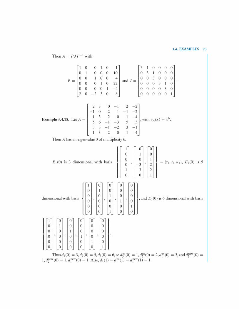
3.4. EXAMPLES 73
Then A = PJP −1 with
P =
⎡⎢⎢⎢⎢⎢⎢⎢⎣
1 0 0 1 0 10 1 0 0 0 100 0 1 0 0 40 0 0 1 0 220 0 0 0 1 −42 0 −2 3 0 8
⎤⎥⎥⎥⎥⎥⎥⎥⎦
and J =
⎡⎢⎢⎢⎢⎢⎢⎢⎣
3 1 0 0 0 00 3 1 0 0 00 0 3 0 0 00 0 0 3 1 00 0 0 0 3 00 0 0 0 0 1
⎤⎥⎥⎥⎥⎥⎥⎥⎦
.
Example 3.4.15. Let A =
⎡⎢⎢⎢⎢⎢⎢⎢⎣
2 3 0 −1 2 −2−1 0 2 1 −1 −2
1 3 2 0 1 −45 6 −1 −3 5 33 3 −1 −2 3 −11 3 2 0 1 −4
⎤⎥⎥⎥⎥⎥⎥⎥⎦
, with cA(x) = x6.
Then A has an eigenvalue 0 of multiplicity 6.
E1(0) is 3 dimensional with basis
⎧⎪⎪⎪⎪⎪⎪⎪⎨⎪⎪⎪⎪⎪⎪⎪⎩
⎡⎢⎢⎢⎢⎢⎢⎢⎣
1000
−10
⎤⎥⎥⎥⎥⎥⎥⎥⎦
,
⎡⎢⎢⎢⎢⎢⎢⎢⎣
010
−3−3
0
⎤⎥⎥⎥⎥⎥⎥⎥⎦
,
⎡⎢⎢⎢⎢⎢⎢⎢⎣
001221
⎤⎥⎥⎥⎥⎥⎥⎥⎦
⎫⎪⎪⎪⎪⎪⎪⎪⎬⎪⎪⎪⎪⎪⎪⎪⎭
= {s1, t1, u1}, E2(0) is 5
dimensional with basis
⎧⎪⎪⎪⎪⎪⎪⎪⎨⎪⎪⎪⎪⎪⎪⎪⎩
⎡⎢⎢⎢⎢⎢⎢⎢⎣
100000
⎤⎥⎥⎥⎥⎥⎥⎥⎦
,
⎡⎢⎢⎢⎢⎢⎢⎢⎣
010000
⎤⎥⎥⎥⎥⎥⎥⎥⎦
,
⎡⎢⎢⎢⎢⎢⎢⎢⎣
001001
⎤⎥⎥⎥⎥⎥⎥⎥⎦
,
⎡⎢⎢⎢⎢⎢⎢⎢⎣
000100
⎤⎥⎥⎥⎥⎥⎥⎥⎦
,
⎡⎢⎢⎢⎢⎢⎢⎢⎣
000010
⎤⎥⎥⎥⎥⎥⎥⎥⎦
⎫⎪⎪⎪⎪⎪⎪⎪⎬⎪⎪⎪⎪⎪⎪⎪⎭
, and E3(0) is 6 dimensional with basis
⎧⎪⎪⎪⎪⎪⎪⎪⎨⎪⎪⎪⎪⎪⎪⎪⎩
⎡⎢⎢⎢⎢⎢⎢⎢⎣
100000
⎤⎥⎥⎥⎥⎥⎥⎥⎦
,
⎡⎢⎢⎢⎢⎢⎢⎢⎣
010000
⎤⎥⎥⎥⎥⎥⎥⎥⎦
,
⎡⎢⎢⎢⎢⎢⎢⎢⎣
001000
⎤⎥⎥⎥⎥⎥⎥⎥⎦
,
⎡⎢⎢⎢⎢⎢⎢⎢⎣
000100
⎤⎥⎥⎥⎥⎥⎥⎥⎦
,
⎡⎢⎢⎢⎢⎢⎢⎢⎣
000010
⎤⎥⎥⎥⎥⎥⎥⎥⎦
,
⎡⎢⎢⎢⎢⎢⎢⎢⎣
000001
⎤⎥⎥⎥⎥⎥⎥⎥⎦
⎫⎪⎪⎪⎪⎪⎪⎪⎬⎪⎪⎪⎪⎪⎪⎪⎭
.
Thus d1(0) = 3, d2(0) = 5, d3(0) = 6, so dex3 (0) = 1, dex
2 (0) = 2, dex1 (0) = 3, and dnew
3 (0) =1, dnew
2 (0) = 1, dnew1 (0) = 1. Also, d1(1) = dex
1 (1) = dnew1 (1) = 1.
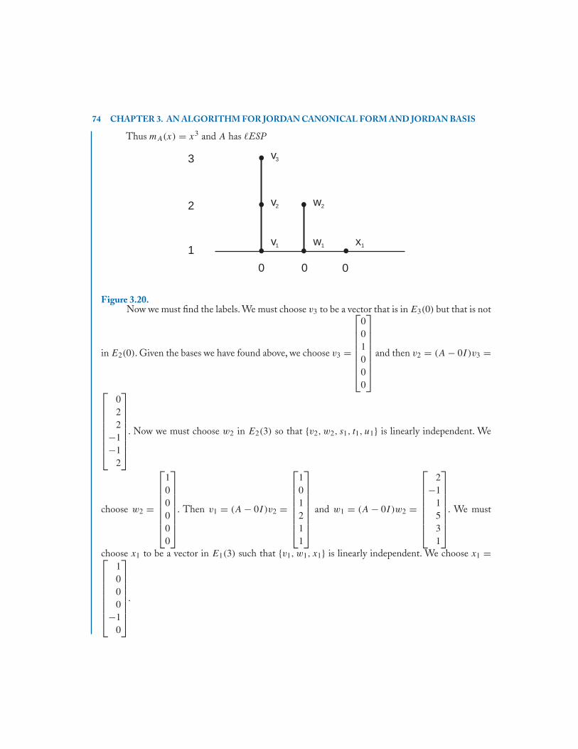
74 CHAPTER 3. AN ALGORITHM FOR JORDAN CANONICAL FORM AND JORDAN BASIS
Thus mA(x) = x3 and A has �ESP
3
2
1
v3
v2
v
0 0
1
w2
w1 x1
0
Figure 3.20.Now we must find the labels. We must choose v3 to be a vector that is in E3(0) but that is not
in E2(0). Given the bases we have found above, we choose v3 =
⎡⎢⎢⎢⎢⎢⎢⎢⎣
001000
⎤⎥⎥⎥⎥⎥⎥⎥⎦
and then v2 = (A − 0I )v3 =
⎡⎢⎢⎢⎢⎢⎢⎢⎣
022
−1−1
2
⎤⎥⎥⎥⎥⎥⎥⎥⎦
. Now we must choose w2 in E2(3) so that {v2, w2, s1, t1, u1} is linearly independent. We
choose w2 =
⎡⎢⎢⎢⎢⎢⎢⎢⎣
100000
⎤⎥⎥⎥⎥⎥⎥⎥⎦
. Then v1 = (A − 0I )v2 =
⎡⎢⎢⎢⎢⎢⎢⎢⎣
101211
⎤⎥⎥⎥⎥⎥⎥⎥⎦
and w1 = (A − 0I )w2 =
⎡⎢⎢⎢⎢⎢⎢⎢⎣
2−1
1531
⎤⎥⎥⎥⎥⎥⎥⎥⎦
. We must
choose x1 to be a vector in E1(3) such that {v1, w1, x1} is linearly independent. We choose x1 =⎡⎢⎢⎢⎢⎢⎢⎢⎣
1000
−10
⎤⎥⎥⎥⎥⎥⎥⎥⎦
.
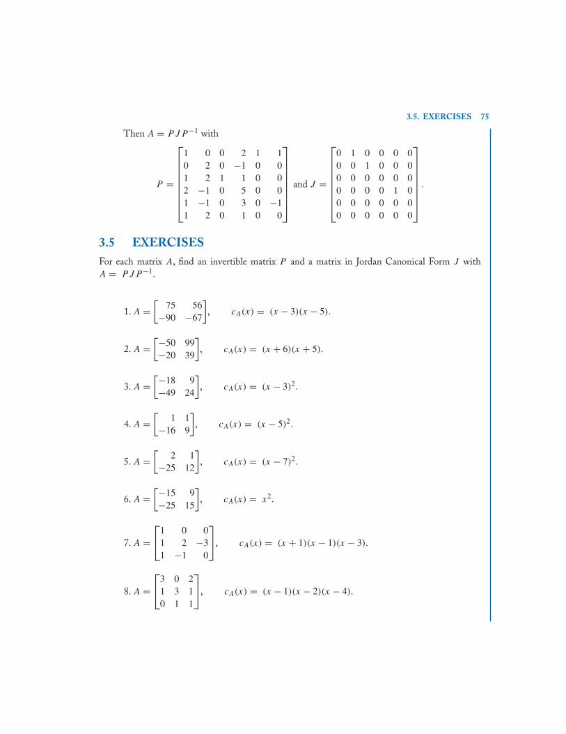
3.5. EXERCISES 75
Then A = PJP −1 with
P =
⎡⎢⎢⎢⎢⎢⎢⎢⎣
1 0 0 2 1 10 2 0 −1 0 01 2 1 1 0 02 −1 0 5 0 01 −1 0 3 0 −11 2 0 1 0 0
⎤⎥⎥⎥⎥⎥⎥⎥⎦
and J =
⎡⎢⎢⎢⎢⎢⎢⎢⎣
0 1 0 0 0 00 0 1 0 0 00 0 0 0 0 00 0 0 0 1 00 0 0 0 0 00 0 0 0 0 0
⎤⎥⎥⎥⎥⎥⎥⎥⎦
.
3.5 EXERCISESFor each matrix A, find an invertible matrix P and a matrix in Jordan Canonical Form J withA = PJP −1.
1. A =[
75 56−90 −67
], cA(x) = (x − 3)(x − 5).
2. A =[−50 99−20 39
], cA(x) = (x + 6)(x + 5).
3. A =[−18 9−49 24
], cA(x) = (x − 3)2.
4. A =[
1 1−16 9
], cA(x) = (x − 5)2.
5. A =[
2 1−25 12
], cA(x) = (x − 7)2.
6. A =[−15 9−25 15
], cA(x) = x2.
7. A =⎡⎣1 0 0
1 2 −31 −1 0
⎤⎦, cA(x) = (x + 1)(x − 1)(x − 3).
8. A =⎡⎣3 0 2
1 3 10 1 1
⎤⎦, cA(x) = (x − 1)(x − 2)(x − 4).
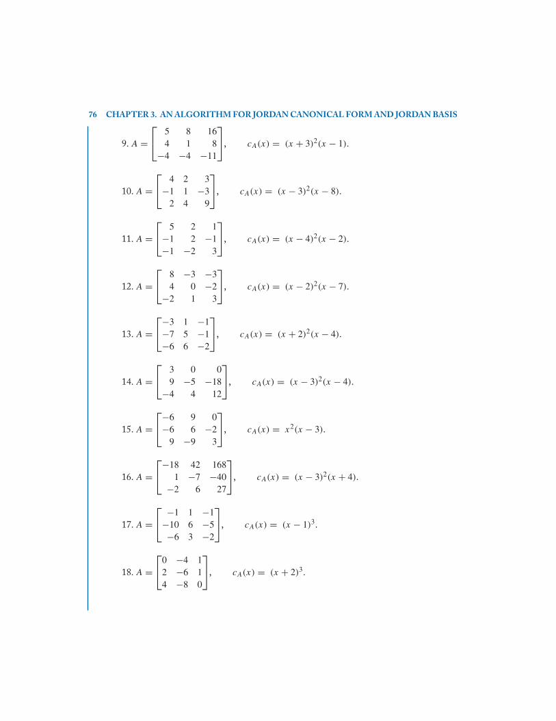
76 CHAPTER 3. AN ALGORITHM FOR JORDAN CANONICAL FORM AND JORDAN BASIS
9. A =⎡⎣ 5 8 16
4 1 8−4 −4 −11
⎤⎦, cA(x) = (x + 3)2(x − 1).
10. A =⎡⎣ 4 2 3
−1 1 −32 4 9
⎤⎦, cA(x) = (x − 3)2(x − 8).
11. A =⎡⎣ 5 2 1
−1 2 −1−1 −2 3
⎤⎦, cA(x) = (x − 4)2(x − 2).
12. A =⎡⎣ 8 −3 −3
4 0 −2−2 1 3
⎤⎦, cA(x) = (x − 2)2(x − 7).
13. A =⎡⎣−3 1 −1
−7 5 −1−6 6 −2
⎤⎦, cA(x) = (x + 2)2(x − 4).
14. A =⎡⎣ 3 0 0
9 −5 −18−4 4 12
⎤⎦, cA(x) = (x − 3)2(x − 4).
15. A =⎡⎣−6 9 0
−6 6 −29 −9 3
⎤⎦, cA(x) = x2(x − 3).
16. A =⎡⎣−18 42 168
1 −7 −40−2 6 27
⎤⎦, cA(x) = (x − 3)2(x + 4).
17. A =⎡⎣ −1 1 −1
−10 6 −5−6 3 −2
⎤⎦, cA(x) = (x − 1)3.
18. A =⎡⎣0 −4 1
2 −6 14 −8 0
⎤⎦, cA(x) = (x + 2)3.
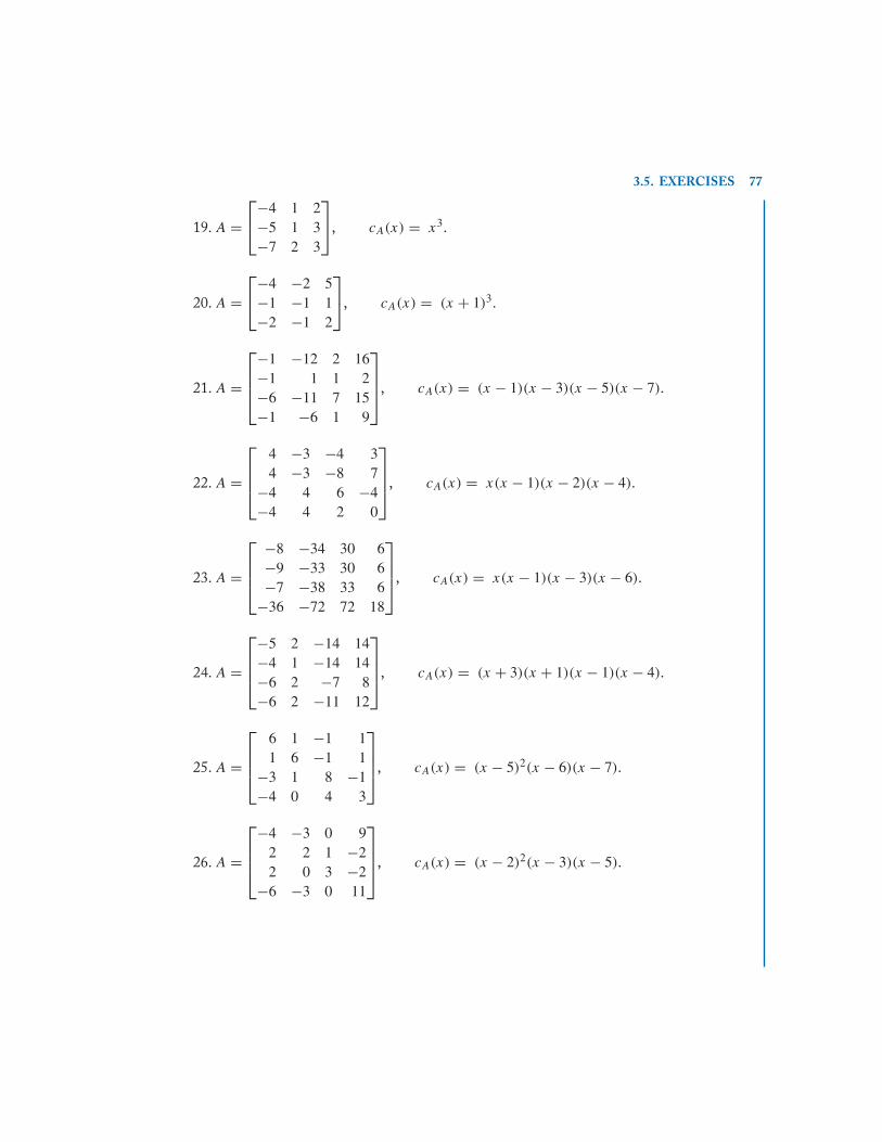
3.5. EXERCISES 77
19. A =⎡⎣−4 1 2
−5 1 3−7 2 3
⎤⎦, cA(x) = x3.
20. A =⎡⎣−4 −2 5
−1 −1 1−2 −1 2
⎤⎦, cA(x) = (x + 1)3.
21. A =
⎡⎢⎢⎣
−1 −12 2 16−1 1 1 2−6 −11 7 15−1 −6 1 9
⎤⎥⎥⎦, cA(x) = (x − 1)(x − 3)(x − 5)(x − 7).
22. A =
⎡⎢⎢⎣
4 −3 −4 34 −3 −8 7
−4 4 6 −4−4 4 2 0
⎤⎥⎥⎦, cA(x) = x(x − 1)(x − 2)(x − 4).
23. A =
⎡⎢⎢⎣
−8 −34 30 6−9 −33 30 6−7 −38 33 6
−36 −72 72 18
⎤⎥⎥⎦, cA(x) = x(x − 1)(x − 3)(x − 6).
24. A =
⎡⎢⎢⎣
−5 2 −14 14−4 1 −14 14−6 2 −7 8−6 2 −11 12
⎤⎥⎥⎦, cA(x) = (x + 3)(x + 1)(x − 1)(x − 4).
25. A =
⎡⎢⎢⎣
6 1 −1 11 6 −1 1
−3 1 8 −1−4 0 4 3
⎤⎥⎥⎦, cA(x) = (x − 5)2(x − 6)(x − 7).
26. A =
⎡⎢⎢⎣
−4 −3 0 92 2 1 −22 0 3 −2
−6 −3 0 11
⎤⎥⎥⎦, cA(x) = (x − 2)2(x − 3)(x − 5).
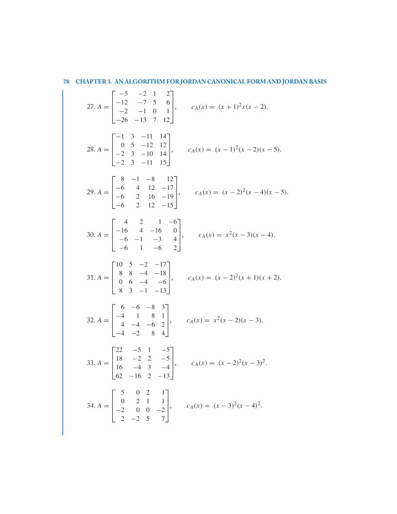
78 CHAPTER 3. AN ALGORITHM FOR JORDAN CANONICAL FORM AND JORDAN BASIS
27. A =
⎡⎢⎢⎣
−5 −2 1 2−12 −7 5 6−2 −1 0 1
−26 −13 7 12
⎤⎥⎥⎦, cA(x) = (x + 1)2x(x − 2).
28. A =
⎡⎢⎢⎣
−1 3 −11 140 5 −12 12
−2 3 −10 14−2 3 −11 15
⎤⎥⎥⎦, cA(x) = (x − 1)2(x − 2)(x − 5).
29. A =
⎡⎢⎢⎣
8 −1 −8 12−6 4 12 −17−6 2 16 −19−6 2 12 −15
⎤⎥⎥⎦, cA(x) = (x − 2)2(x − 4)(x − 5).
30. A =
⎡⎢⎢⎣
4 2 1 −6−16 4 −16 0−6 −1 −3 4−6 1 −6 2
⎤⎥⎥⎦, cA(x) = x2(x − 3)(x − 4).
31. A =
⎡⎢⎢⎣
10 5 −2 −178 8 −4 −180 6 −4 −68 3 −1 −13
⎤⎥⎥⎦, cA(x) = (x − 2)2(x + 1)(x + 2).
32. A =
⎡⎢⎢⎣
6 −6 −8 3−4 1 8 1
4 −4 −6 2−4 −2 8 4
⎤⎥⎥⎦, cA(x) = x2(x − 2)(x − 3).
33. A =
⎡⎢⎢⎣
22 −5 1 −518 −2 2 −516 −4 3 −462 −16 2 −13
⎤⎥⎥⎦, cA(x) = (x − 2)2(x − 3)2.
34. A =
⎡⎢⎢⎣
5 0 2 10 2 1 1
−2 0 0 −22 −2 5 7
⎤⎥⎥⎦, cA(x) = (x − 3)2(x − 4)2.
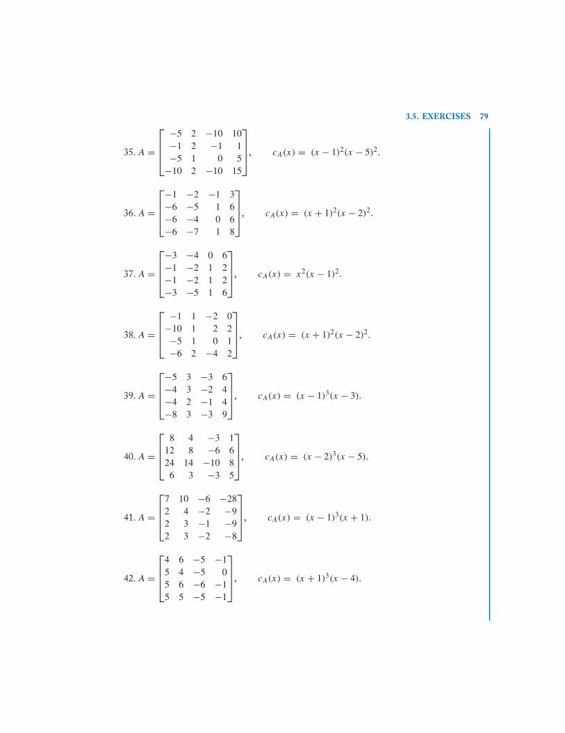
3.5. EXERCISES 79
35. A =
⎡⎢⎢⎣
−5 2 −10 10−1 2 −1 1−5 1 0 5
−10 2 −10 15
⎤⎥⎥⎦, cA(x) = (x − 1)2(x − 5)2.
36. A =
⎡⎢⎢⎣
−1 −2 −1 3−6 −5 1 6−6 −4 0 6−6 −7 1 8
⎤⎥⎥⎦, cA(x) = (x + 1)2(x − 2)2.
37. A =
⎡⎢⎢⎣
−3 −4 0 6−1 −2 1 2−1 −2 1 2−3 −5 1 6
⎤⎥⎥⎦, cA(x) = x2(x − 1)2.
38. A =
⎡⎢⎢⎣
−1 1 −2 0−10 1 2 2−5 1 0 1−6 2 −4 2
⎤⎥⎥⎦, cA(x) = (x + 1)2(x − 2)2.
39. A =
⎡⎢⎢⎣
−5 3 −3 6−4 3 −2 4−4 2 −1 4−8 3 −3 9
⎤⎥⎥⎦, cA(x) = (x − 1)3(x − 3).
40. A =
⎡⎢⎢⎣
8 4 −3 112 8 −6 624 14 −10 8
6 3 −3 5
⎤⎥⎥⎦, cA(x) = (x − 2)3(x − 5).
41. A =
⎡⎢⎢⎣
7 10 −6 −282 4 −2 −92 3 −1 −92 3 −2 −8
⎤⎥⎥⎦, cA(x) = (x − 1)3(x + 1).
42. A =
⎡⎢⎢⎣
4 6 −5 −15 4 −5 05 6 −6 −15 5 −5 −1
⎤⎥⎥⎦, cA(x) = (x + 1)3(x − 4).
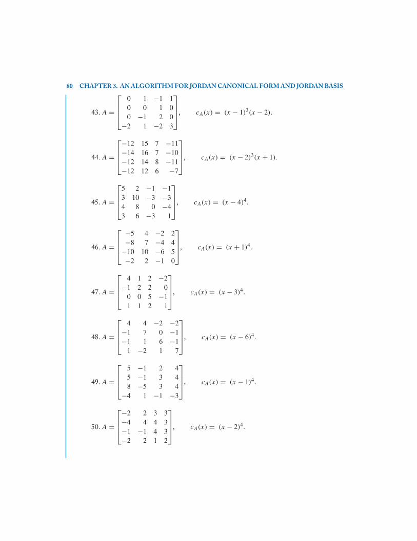
80 CHAPTER 3. AN ALGORITHM FOR JORDAN CANONICAL FORM AND JORDAN BASIS
43. A =
⎡⎢⎢⎣
0 1 −1 10 0 1 00 −1 2 0
−2 1 −2 3
⎤⎥⎥⎦, cA(x) = (x − 1)3(x − 2).
44. A =
⎡⎢⎢⎣
−12 15 7 −11−14 16 7 −10−12 14 8 −11−12 12 6 −7
⎤⎥⎥⎦, cA(x) = (x − 2)3(x + 1).
45. A =
⎡⎢⎢⎣
5 2 −1 −13 10 −3 −34 8 0 −43 6 −3 1
⎤⎥⎥⎦, cA(x) = (x − 4)4.
46. A =
⎡⎢⎢⎣
−5 4 −2 2−8 7 −4 4
−10 10 −6 5−2 2 −1 0
⎤⎥⎥⎦, cA(x) = (x + 1)4.
47. A =
⎡⎢⎢⎣
4 1 2 −2−1 2 2 0
0 0 5 −11 1 2 1
⎤⎥⎥⎦, cA(x) = (x − 3)4.
48. A =
⎡⎢⎢⎣
4 4 −2 −2−1 7 0 −1−1 1 6 −1
1 −2 1 7
⎤⎥⎥⎦, cA(x) = (x − 6)4.
49. A =
⎡⎢⎢⎣
5 −1 2 45 −1 3 48 −5 3 4
−4 1 −1 −3
⎤⎥⎥⎦, cA(x) = (x − 1)4.
50. A =
⎡⎢⎢⎣
−2 2 3 3−4 4 4 3−1 −1 4 3−2 2 1 2
⎤⎥⎥⎦, cA(x) = (x − 2)4.

3.5. EXERCISES 81
51. A =
⎡⎢⎢⎣
2 −3 −2 3−4 2 4 −4−4 0 4 −3−8 4 8 −8
⎤⎥⎥⎦, cA(x) = x4.
52. A =
⎡⎢⎢⎣
1 3 −6 0−2 3 −4 6−1 1 −1 3
0 1 −2 1
⎤⎥⎥⎦, cA(x) = (x − 1)4.
53. A =
⎡⎢⎢⎢⎢⎣
−5 −2 0 −4 82 1 −2 2 0
−3 −1 −2 −3 8−1 −1 1 −2 0−4 −1 0 −2 7
⎤⎥⎥⎥⎥⎦, cA(x) = (x + 1)4(x − 3).
54. A =
⎡⎢⎢⎢⎢⎣
−1 1 −4 2 4−1 −1 2 2 0−1 −1 2 2 0
0 1 −3 0 2−1 −1 0 2 2
⎤⎥⎥⎥⎥⎦, cA(x) = x4(x − 2).
55. A =
⎡⎢⎢⎢⎢⎣
5 1 3 −1 −33 1 4 1 −30 −4 4 4 03 1 3 1 −36 −3 8 3 −4
⎤⎥⎥⎥⎥⎦, cA(x) = (x − 2)4(x + 1).
56. A =
⎡⎢⎢⎢⎢⎣
5 1 0 0 −21 6 1 −2 −21 2 5 −2 −21 2 1 2 −22 1 0 0 1
⎤⎥⎥⎥⎥⎦, cA(x) = (x − 4)4(x − 3).
57. A =
⎡⎢⎢⎢⎢⎣
−2 −9 −10 −7 108 21 21 15 −20
−2 −1 1 0 0−8 −18 −20 −12 20−2 −5 −5 −4 7
⎤⎥⎥⎥⎥⎦, cA(x) = (x − 2)4(x − 7).

82 CHAPTER 3. AN ALGORITHM FOR JORDAN CANONICAL FORM AND JORDAN BASIS
58. A =
⎡⎢⎢⎢⎢⎣
−1 2 4 2 −1−3 5 4 1 −1−1 0 4 1 0−3 2 3 4 −1−2 1 3 1 2
⎤⎥⎥⎥⎥⎦, cA(x) = (x − 3)4(x − 2).
59. A =
⎡⎢⎢⎢⎢⎢⎢⎢⎣
5 7 5 2 −2 −82 10 7 2 −3 −7
−2 −7 −4 −2 3 70 0 −1 3 1 0
−2 −7 −7 −2 6 72 6 5 2 −2 −4
⎤⎥⎥⎥⎥⎥⎥⎥⎦
, cA(x) = (x − 3)5(x − 1).
60. A =
⎡⎢⎢⎢⎢⎢⎢⎢⎣
9 3 0 3 −3 −120 3 3 1 −2 00 −2 8 1 −2 00 −1 0 4 2 00 −2 2 0 5 02 1 0 1 −1 −1
⎤⎥⎥⎥⎥⎥⎥⎥⎦
, cA(x) = (x − 5)5(x − 3).

83
A P P E N D I X A
Answers to odd-numberedexercises
A.1 ANSWERS TO EXERCISES–CHAPTER 2
1. J =
⎡⎢⎢⎣
2 0 0 00 3 0 00 0 5 00 0 0 7
⎤⎥⎥⎦, mA(x) = (x − 2)(x − 3)(x − 5)(x − 7),
alg-mult(2) = 1, geom-mult(2) = 1, max-ind(2) = 1,alg-mult(3) = 1, geom-mult(3) = 1, max-ind(3) = 1,alg-mult(5) = 1, geom-mult(5) = 1, max-ind(5) = 1,alg-mult(7) = 1, geom-mult(7) = 1, max-ind(7) = 1.
3. J =
⎡⎢⎢⎢⎢⎣
2 1 0 0 00 2 1 0 00 0 2 0 00 0 0 3 10 0 0 0 3
⎤⎥⎥⎥⎥⎦, mA(x) = (x − 2)3(x − 3)2,
alg-mult(2) = 3, geom-mult(2) = 1, max-ind(2) = 3,alg-mult(3) = 2, geom-mult(3) = 1, max-ind(3) = 2;
J =
⎡⎢⎢⎢⎢⎣
2 1 0 0 00 2 1 0 00 0 2 0 00 0 0 3 00 0 0 0 3
⎤⎥⎥⎥⎥⎦, mA(x) = (x − 2)3(x − 3),
alg-mult(2) = 3, geom-mult(2) = 1, max-ind(2) = 3,alg-mult(3) = 2, geom-mult(3) = 2, max-ind(3) = 1;
J =
⎡⎢⎢⎢⎢⎣
2 1 0 0 00 2 0 0 00 0 2 0 00 0 0 3 10 0 0 0 3
⎤⎥⎥⎥⎥⎦, mA(x) = (x − 2)2(x − 3)2,
alg-mult(2) = 3, geom-mult(2) = 2, max-ind(2) = 2,alg-mult(3) = 2, geom-mult(3) = 1, max-ind(3) = 2;

84 APPENDIX A. ANSWERS TO ODD-NUMBERED EXERCISES
J =
⎡⎢⎢⎢⎢⎣
2 1 0 0 00 2 0 0 00 0 2 0 00 0 0 3 00 0 0 0 3
⎤⎥⎥⎥⎥⎦, mA(x) = (x − 2)2(x − 3)2,
alg-mult(2) = 3, geom-mult(2) = 2, max-ind(2) = 2,alg-mult(3) = 2, geom-mult(3) = 2, max-ind(3) = 1;
J =
⎡⎢⎢⎢⎢⎣
2 0 0 0 00 2 0 0 00 0 2 0 00 0 0 3 10 0 0 0 3
⎤⎥⎥⎥⎥⎦, mA(x) = (x − 2)(x − 3)2,
alg-mult(2) = 3, geom-mult(2) = 3, max-ind(2) = 1,alg-mult(3) = 2, geom-mult(3) = 1, max-ind(3) = 2;
J =
⎡⎢⎢⎢⎢⎣
2 0 0 0 00 2 0 0 00 0 2 0 00 0 0 3 00 0 0 0 3
⎤⎥⎥⎥⎥⎦, mA(x) = (x − 2)(x − 3),
alg-mult(2) = 3, geom-mult(2) = 3, max-ind(2) = 1,alg-mult(3) = 2, geom-mult(3) = 2, max-ind(3) = 1.
5. J =
⎡⎢⎢⎢⎢⎢⎢⎢⎢⎢⎢⎢⎣
3 1 0 0 0 0 0 00 3 0 0 0 0 0 00 0 3 1 0 0 0 00 0 0 3 0 0 0 00 0 0 0 5 1 0 00 0 0 0 0 5 0 00 0 0 0 0 0 5 10 0 0 0 0 0 0 5
⎤⎥⎥⎥⎥⎥⎥⎥⎥⎥⎥⎥⎦
,
alg-mult(3) = 4, geom-mult(3) = 2, max-ind(3) = 2,alg-mult(5) = 4, geom-mult(5) = 2, max-ind(5) = 2;

A.1. ANSWERS TO EXERCISES–CHAPTER 2 85
J =
⎡⎢⎢⎢⎢⎢⎢⎢⎢⎢⎢⎢⎣
3 1 0 0 0 0 0 00 3 0 0 0 0 0 00 0 3 1 0 0 0 00 0 0 3 0 0 0 00 0 0 0 5 1 0 00 0 0 0 0 5 0 00 0 0 0 0 0 5 00 0 0 0 0 0 0 5
⎤⎥⎥⎥⎥⎥⎥⎥⎥⎥⎥⎥⎦
,
alg-mult(3) = 4, geom-mult(3) = 2, max-ind(3) = 2,alg-mult(5) = 4, geom-mult(5) = 3, max-ind(5) = 2;
J =
⎡⎢⎢⎢⎢⎢⎢⎢⎢⎢⎢⎢⎣
3 1 0 0 0 0 0 00 3 0 0 0 0 0 00 0 3 0 0 0 0 00 0 0 3 0 0 0 00 0 0 0 5 1 0 00 0 0 0 0 5 0 00 0 0 0 0 0 5 10 0 0 0 0 0 0 5
⎤⎥⎥⎥⎥⎥⎥⎥⎥⎥⎥⎥⎦
,
alg-mult(3) = 4, geom-mult(3) = 3, max-ind(3) = 2,alg-mult(5) = 4, geom-mult(5) = 2, max-ind(5) = 2;
J =
⎡⎢⎢⎢⎢⎢⎢⎢⎢⎢⎢⎢⎣
3 1 0 0 0 0 0 00 3 0 0 0 0 0 00 0 3 0 0 0 0 00 0 0 3 0 0 0 00 0 0 0 5 1 0 00 0 0 0 0 5 0 00 0 0 0 0 0 5 00 0 0 0 0 0 0 5
⎤⎥⎥⎥⎥⎥⎥⎥⎥⎥⎥⎥⎦
,
alg-mult(3) = 4, geom-mult(3) = 3, max-ind(3) = 2,alg-mult(5) = 4, geom-mult(5) = 3, max-ind(5) = 2.
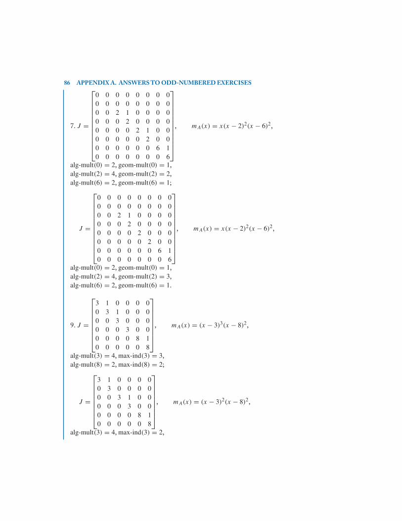
86 APPENDIX A. ANSWERS TO ODD-NUMBERED EXERCISES
7. J =
⎡⎢⎢⎢⎢⎢⎢⎢⎢⎢⎢⎢⎣
0 0 0 0 0 0 0 00 0 0 0 0 0 0 00 0 2 1 0 0 0 00 0 0 2 0 0 0 00 0 0 0 2 1 0 00 0 0 0 0 2 0 00 0 0 0 0 0 6 10 0 0 0 0 0 0 6
⎤⎥⎥⎥⎥⎥⎥⎥⎥⎥⎥⎥⎦
, mA(x) = x(x − 2)2(x − 6)2,
alg-mult(0) = 2, geom-mult(0) = 1,alg-mult(2) = 4, geom-mult(2) = 2,alg-mult(6) = 2, geom-mult(6) = 1;
J =
⎡⎢⎢⎢⎢⎢⎢⎢⎢⎢⎢⎢⎣
0 0 0 0 0 0 0 00 0 0 0 0 0 0 00 0 2 1 0 0 0 00 0 0 2 0 0 0 00 0 0 0 2 0 0 00 0 0 0 0 2 0 00 0 0 0 0 0 6 10 0 0 0 0 0 0 6
⎤⎥⎥⎥⎥⎥⎥⎥⎥⎥⎥⎥⎦
, mA(x) = x(x − 2)2(x − 6)2,
alg-mult(0) = 2, geom-mult(0) = 1,alg-mult(2) = 4, geom-mult(2) = 3,alg-mult(6) = 2, geom-mult(6) = 1.
9. J =
⎡⎢⎢⎢⎢⎢⎢⎢⎣
3 1 0 0 0 00 3 1 0 0 00 0 3 0 0 00 0 0 3 0 00 0 0 0 8 10 0 0 0 0 8
⎤⎥⎥⎥⎥⎥⎥⎥⎦
, mA(x) = (x − 3)3(x − 8)2,
alg-mult(3) = 4, max-ind(3) = 3,alg-mult(8) = 2, max-ind(8) = 2;
J =
⎡⎢⎢⎢⎢⎢⎢⎢⎣
3 1 0 0 0 00 3 0 0 0 00 0 3 1 0 00 0 0 3 0 00 0 0 0 8 10 0 0 0 0 8
⎤⎥⎥⎥⎥⎥⎥⎥⎦
, mA(x) = (x − 3)2(x − 8)2,
alg-mult(3) = 4, max-ind(3) = 2,

A.1. ANSWERS TO EXERCISES–CHAPTER 2 87
alg-mult(8) = 2, max-ind(8) = 2.
11. J =
⎡⎢⎢⎢⎢⎢⎢⎢⎣
1 1 0 0 0 00 1 1 0 0 00 0 1 1 0 00 0 0 1 0 00 0 0 0 1 00 0 0 0 0 4
⎤⎥⎥⎥⎥⎥⎥⎥⎦
, cA(x) = (x − 1)5(x − 4),
alg-mult(1) = 5, geom-mult(1) = 2, max-ind(1) = 4,alg-mult(4) = 1, geom-mult(4) = 1, max-ind(4) = 1;
J =
⎡⎢⎢⎢⎢⎢⎢⎢⎣
1 1 0 0 0 00 1 1 0 0 00 0 1 1 0 00 0 0 1 0 00 0 0 0 4 00 0 0 0 0 4
⎤⎥⎥⎥⎥⎥⎥⎥⎦
, cA(x) = (x − 1)4(x − 4)2,
alg-mult(1) = 4, geom-mult(1) = 1, max-ind(1) = 4,alg-mult(4) = 2, geom-mult(4) = 2, max-ind(4) = 1.
13. J =
⎡⎢⎢⎢⎢⎣
1 1 0 0 00 1 1 0 00 0 1 0 00 0 0 1 00 0 0 0 1
⎤⎥⎥⎥⎥⎦, cA(x) = (x − 1)5, mA(x) = (x − 1)3,
max-ind(1) = 3;
J =
⎡⎢⎢⎢⎢⎣
1 1 0 0 00 1 0 0 00 0 1 1 00 0 0 1 00 0 0 0 1
⎤⎥⎥⎥⎥⎦, cA(x) = (x − 1)5, mA(x) = (x − 1)2,
max-ind(1) = 2.
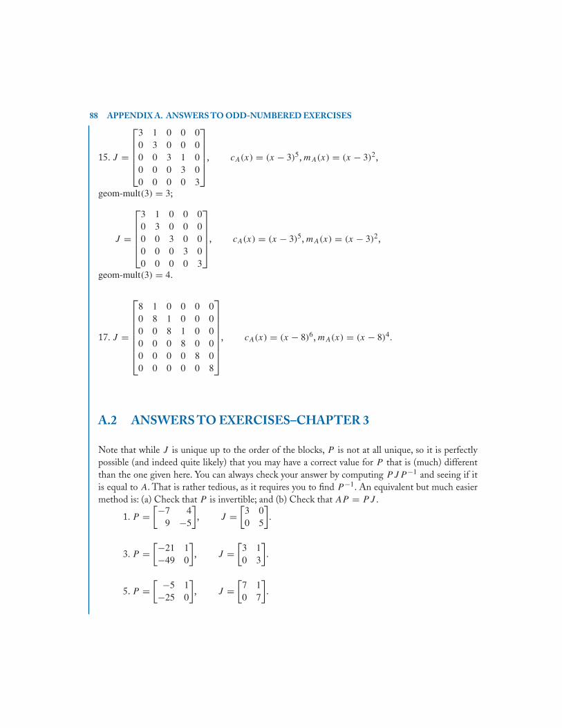
88 APPENDIX A. ANSWERS TO ODD-NUMBERED EXERCISES
15. J =
⎡⎢⎢⎢⎢⎣
3 1 0 0 00 3 0 0 00 0 3 1 00 0 0 3 00 0 0 0 3
⎤⎥⎥⎥⎥⎦, cA(x) = (x − 3)5, mA(x) = (x − 3)2,
geom-mult(3) = 3;
J =
⎡⎢⎢⎢⎢⎣
3 1 0 0 00 3 0 0 00 0 3 0 00 0 0 3 00 0 0 0 3
⎤⎥⎥⎥⎥⎦, cA(x) = (x − 3)5, mA(x) = (x − 3)2,
geom-mult(3) = 4.
17. J =
⎡⎢⎢⎢⎢⎢⎢⎢⎣
8 1 0 0 0 00 8 1 0 0 00 0 8 1 0 00 0 0 8 0 00 0 0 0 8 00 0 0 0 0 8
⎤⎥⎥⎥⎥⎥⎥⎥⎦
, cA(x) = (x − 8)6, mA(x) = (x − 8)4.
A.2 ANSWERS TO EXERCISES–CHAPTER 3
Note that while J is unique up to the order of the blocks, P is not at all unique, so it is perfectlypossible (and indeed quite likely) that you may have a correct value for P that is (much) differentthan the one given here. You can always check your answer by computing PJP −1 and seeing if itis equal to A. That is rather tedious, as it requires you to find P −1. An equivalent but much easiermethod is: (a) Check that P is invertible; and (b) Check that AP = PJ .
1. P =[−7 4
9 −5
], J =
[3 00 5
].
3. P =[−21 1−49 0
], J =
[3 10 3
].
5. P =[ −5 1−25 0
], J =
[7 10 7
].

A.2. ANSWERS TO EXERCISES–CHAPTER 3 89
7. P =⎡⎣0 2 0
1 1 −31 1 1
⎤⎦, J =
⎡⎣−1 0 0
0 1 00 0 3
⎤⎦.
9. P =⎡⎣−1 −2 −2
1 0 −10 1 1
⎤⎦, J =
⎡⎣−3 0 0
0 −3 00 0 1
⎤⎦.
11. P =⎡⎣−1 −2 −1
0 1 11 0 1
⎤⎦, J =
⎡⎣4 0 0
0 4 00 0 2
⎤⎦.
13. P =⎡⎣−1 0 0
−1 0 10 1 1
⎤⎦, J =
⎡⎣−2 1 0
0 −2 00 0 4
⎤⎦.
15. P =⎡⎣−3 −1 −2
−2 −1 −23 1 3
⎤⎦, J =
⎡⎣0 1 0
0 0 00 0 3
⎤⎦.
17. P =⎡⎣ −2 1 1
−10 0 2−6 0 0
⎤⎦, J =
⎡⎣1 1 0
0 1 00 0 1
⎤⎦.
19. P =⎡⎣1 2 0
2 3 01 3 1
⎤⎦, J =
⎡⎣0 1 0
0 0 10 0 0
⎤⎦.
21. P =
⎡⎢⎢⎣
1 2 2 220 1 1 31 2 4 180 1 1 11
⎤⎥⎥⎦, J =
⎡⎢⎢⎣
1 0 0 00 3 0 00 0 5 00 0 0 7
⎤⎥⎥⎦.
23. P =
⎡⎢⎢⎣
1 2 2 11 3 2 11 4 3 12 0 0 3
⎤⎥⎥⎦, J =
⎡⎢⎢⎣
0 0 0 00 1 0 00 0 3 00 0 0 6
⎤⎥⎥⎦.

90 APPENDIX A. ANSWERS TO ODD-NUMBERED EXERCISES
25. P =
⎡⎢⎢⎣
1 0 1 00 1 1 01 1 1 10 −2 0 1
⎤⎥⎥⎦, J =
⎡⎢⎢⎣
5 0 0 00 5 0 00 0 6 00 0 0 7
⎤⎥⎥⎦.
27. P =
⎡⎢⎢⎣
1 0 1 50 1 5 170 0 1 32 1 7 33
⎤⎥⎥⎦, J =
⎡⎢⎢⎣
−1 0 0 00 −1 0 00 0 0 00 0 0 2
⎤⎥⎥⎦.
29. P =
⎡⎢⎢⎣
−2 1 2 14 0 0 −14 −2 1 −14 −2 0 −1
⎤⎥⎥⎦, J =
⎡⎢⎢⎣
2 0 0 00 2 0 00 0 4 00 0 0 5
⎤⎥⎥⎦.
31. P =
⎡⎢⎢⎣
3 0 1 12 1 2 10 1 2 02 0 1 1
⎤⎥⎥⎦, J =
⎡⎢⎢⎣
2 1 0 00 2 0 00 0 −1 00 0 0 −2
⎤⎥⎥⎦.
33. P =
⎡⎢⎢⎣
1 0 1 02 5 4 10 −4 1 02 −6 0 −1
⎤⎥⎥⎦, J =
⎡⎢⎢⎣
2 1 0 00 2 0 00 0 3 00 0 0 3
⎤⎥⎥⎦.
35. P =
⎡⎢⎢⎣
2 0 1 11 1 0 01 0 1 02 0 2 1
⎤⎥⎥⎦, J =
⎡⎢⎢⎣
1 1 0 00 1 0 00 0 5 00 0 0 5
⎤⎥⎥⎦.
37. P =
⎡⎢⎢⎣
2 0 2 10 1 1 00 0 1 01 1 2 1
⎤⎥⎥⎦, J =
⎡⎢⎢⎣
0 1 0 00 0 0 00 0 1 10 0 0 1
⎤⎥⎥⎦.
39. P =
⎡⎢⎢⎣
3 2 1 32 3 1 22 2 1 23 2 1 4
⎤⎥⎥⎦, J =
⎡⎢⎢⎣
1 1 0 00 1 0 00 0 1 00 0 0 3
⎤⎥⎥⎦.
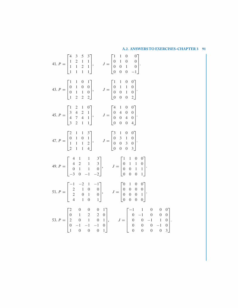
A.2. ANSWERS TO EXERCISES–CHAPTER 3 91
41. P =
⎡⎢⎢⎣
4 3 5 31 2 1 11 1 2 11 1 1 1
⎤⎥⎥⎦, J =
⎡⎢⎢⎣
1 1 0 00 1 0 00 0 1 00 0 0 −1
⎤⎥⎥⎦.
43. P =
⎡⎢⎢⎣
1 1 0 10 1 0 00 1 1 01 2 2 2
⎤⎥⎥⎦, J =
⎡⎢⎢⎣
1 1 0 00 1 1 00 0 1 00 0 0 2
⎤⎥⎥⎦.
45. P =
⎡⎢⎢⎣
1 2 1 03 4 2 14 7 4 13 2 1 1
⎤⎥⎥⎦, J =
⎡⎢⎢⎣
4 1 0 00 4 0 00 0 4 00 0 0 4
⎤⎥⎥⎦.
47. P =
⎡⎢⎢⎣
2 1 1 30 1 0 11 1 1 22 1 1 4
⎤⎥⎥⎦, J =
⎡⎢⎢⎣
3 1 0 00 3 1 00 0 3 00 0 0 3
⎤⎥⎥⎦.
49. P =
⎡⎢⎢⎣
4 1 1 34 2 1 30 1 1 0
−3 0 −1 −2
⎤⎥⎥⎦, J =
⎡⎢⎢⎣
1 1 0 00 1 1 00 0 1 10 0 0 1
⎤⎥⎥⎦.
51. P =
⎡⎢⎢⎣
−1 −2 1 −12 1 0 02 0 1 04 1 0 1
⎤⎥⎥⎦, J =
⎡⎢⎢⎣
0 1 0 00 0 0 00 0 0 10 0 0 0
⎤⎥⎥⎦.
53. P =
⎡⎢⎢⎢⎢⎣
2 0 0 0 10 1 2 2 02 0 1 0 10 −1 −1 −1 01 0 0 0 1
⎤⎥⎥⎥⎥⎦, J =
⎡⎢⎢⎢⎢⎣
−1 1 0 0 00 −1 0 0 00 0 −1 1 00 0 0 −1 00 0 0 0 3
⎤⎥⎥⎥⎥⎦.
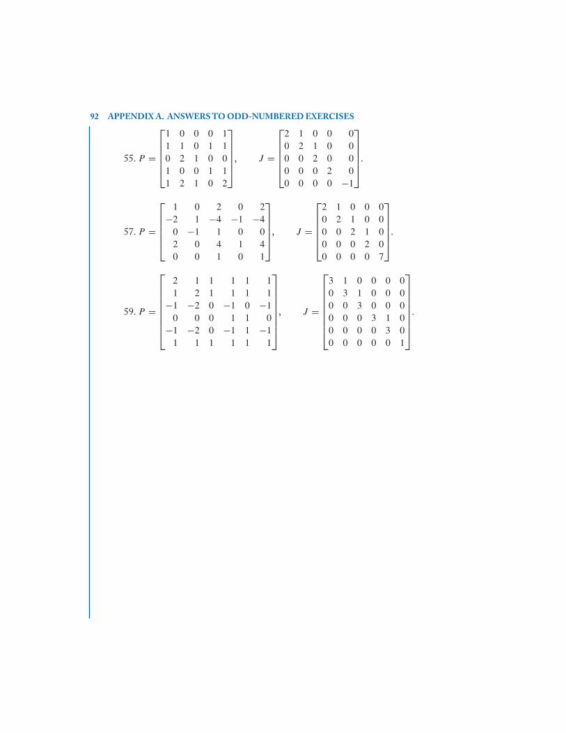
92 APPENDIX A. ANSWERS TO ODD-NUMBERED EXERCISES
55. P =
⎡⎢⎢⎢⎢⎣
1 0 0 0 11 1 0 1 10 2 1 0 01 0 0 1 11 2 1 0 2
⎤⎥⎥⎥⎥⎦, J =
⎡⎢⎢⎢⎢⎣
2 1 0 0 00 2 1 0 00 0 2 0 00 0 0 2 00 0 0 0 −1
⎤⎥⎥⎥⎥⎦.
57. P =
⎡⎢⎢⎢⎢⎣
1 0 2 0 2−2 1 −4 −1 −4
0 −1 1 0 02 0 4 1 40 0 1 0 1
⎤⎥⎥⎥⎥⎦, J =
⎡⎢⎢⎢⎢⎣
2 1 0 0 00 2 1 0 00 0 2 1 00 0 0 2 00 0 0 0 7
⎤⎥⎥⎥⎥⎦.
59. P =
⎡⎢⎢⎢⎢⎢⎢⎢⎣
2 1 1 1 1 11 2 1 1 1 1
−1 −2 0 −1 0 −10 0 0 1 1 0
−1 −2 0 −1 1 −11 1 1 1 1 1
⎤⎥⎥⎥⎥⎥⎥⎥⎦
, J =
⎡⎢⎢⎢⎢⎢⎢⎢⎣
3 1 0 0 0 00 3 1 0 0 00 0 3 0 0 00 0 0 3 1 00 0 0 0 3 00 0 0 0 0 1
⎤⎥⎥⎥⎥⎥⎥⎥⎦
.

93
Notation
∗, 8⊕, 13, 14
alg-mult(λ), 19
C, 1cA(x), 18cT (x), 22
dj (λ), 49dexj (λ), 49
dnewj (λ), 49
E , 2En, 2ei , 2E(λ), 17E∞(λ), 20Ej(λ), 20
geom-mult(λ), 19
I , 4I , 11
jmax, 49
mA(x), 23mT (x), 26max-ind(λ), 22
PC←B, 4
T , 5TA, 5[T ]B, 6[T ]C←B, 6
[v]B, 2


95
Index
BDBSM, 32see matrix
block diagonal with blocks scalarmatrices, 9
BDBUTCDsee matrix
block diagonal whose blocks are uppertriangular with constant diagonal, 9
Cayley-Hamilton Theorem, 29chain of generalized eigenvectors, 34
bottom of, 34top of, 34
characteristic polynomial, 18complement
see subspace, complementary, 13conjugation, 7
diagonalizable, 31, 33direct sum, 13, 14, 30
eigenspace, 17, 22generalized, 20, 22
eigenstructure picture, 44algorithm for, 50labelled, 44
eigenstructure picture, labelledalgorithm for, 55
eigenvalue, 17eigenvector, 17
generalized, 20index of generalized, 20maximum index of generalized, 22
ESPsee eigenstructure picture, 44
factorsirreducible, 25
Fundamental Theorem of Algebra, 1
generalized eigenvectorschain of, 43
intertwinesee matrix, intertwining, 7
JCFsee Jordan Canonical Form, 10
Jordan basis, 39algorithm for, 55
Jordan block, 10, 24, 35, 44Jordan Canonical Form, 10, 17, 36, 38, 39, 44,
45, 50algorithm for, 50
Jordan matrixsee Jordan Canonical Form, 10
�ESPsee eigenstructure picture, labelled, 44
linear transformation, 5matrix of, 6
matrixblock diagonal, 9block diagonal whose blocks are upper
triangular with constant diagonal, 9,26

96 INDEX
block diagonal with blocks scalar matrices,9
block upper triangular, 9change-of-basis, 4diagonal, 8, 45intertwining, 7Jordan Canonical Form, 10nilpotent, 10scalar, 8strictly upper triangular, 10upper triangular, 8upper triangular with constant diagonal, 9
multiplicity, 19algebraic, 19, 31geometric, 19
nilpotencyindex of, 10
node, 43λ, 44
polynomialcharacteristic, 22, 28–30, 38, 39minimum, 23, 26, 30–33, 38, 39
similar, 7subspace, 13
complementary, 13invariant, 15, 16, 21
subspacescomplementary set of, 14
vectorcoordinate, 2
vector spacebasis of, 1