joint reconstruction and motion estimation via nonconvex

Joint reconstruction andmotion estimationvia nonconvex optimizationfor dynamic MRIMASTER THESIS W.A.P. BASTIAANSEN

Faculty of Electrical Engineering, Mathematics and Computer Science (EEMCS)Master program Applied MathematicsSpecialization: Systems Theory, Applied Analysis and Computational Science (SACS)Chair: Applied Analysis

Graduation committee:Prof. dr. S.A. van Gils (UT)Dr. C. Brune (UT)Dr. ir. C.A.T. van den Berg (UMC Utrecht)Prof dr. ir. B.J. Geurts (UT)

Daily supervisorDr. C. BruneDate of presentation16-11-2018

Abstract

Dynamic magnetic resonance imaging (MRI) is a medical imaging technique. MRI reconstruction methodsbuild upon inverse problems, variational methods and optimization in applied mathematcis. To reduce scan-ning time in dynamic MRI, subsampling of the measurements is needed in practice. This typically leads to arte-facts due to missing information. To tackle those artefacts, time-dependent reconstruction methods, whichemploy not only the spatial properties of the image sequence, but also the dynamical information, are verypromising.

In this thesis a joint reconstruction and motion estimation framework is developed and applied to dynamicMRI reconstruction. The optimization of this joint variational model is challenging since it is nonconvex. Cur-rent approaches alternate between the convex subproblems for reconstruction and motion estimation. Thisapproach seems to be working but there is no knowledge about the convergence. To address this problem thefull nonconvex model is optimized via an alternating forward-backward splitting algorithm which is related tothe PALM algorithm for nonconvex optimization.

The performance of joint reconstruction and motion estimation on dynamic MRI is studied. In real medi-cal datasets no ground truth of the flow fields is available. To address this, artificial data from computer vision,with a ground truth for the flow fields at hand, is used to construct a numerical phantom. In combinationwith a 4D XCAT phantom, this offers more insight into the influence of incorporating the motion on the recon-struction quality and choice of optimization method. Finally, the model is applied to experimental medicaldata from the Radiotherapy group of the UMC Utrecht to show its potential for real world scenarios.

3

Acknowledgments

With this master thesis I conclude my time as a student applied mathematics. Six and a half years ago Iexchanged the sunny south of the Netherlands (Brabant!) for the far east. I look back at my time as a studentwith a big smile on my face. I gained a lot of experiences I never thought I would. Running the final stageof the Batavierenrace, being a board member, being part of a ’dispuut’ and so on. For every EC I had to workhard, sometimes because the course was difficult and sometimes because I was giving myself a hard time. Iam proud of what I achieved over the last years and this thesis feels like the cherry on the pie. I would not haveachieved this without the help of many people.

First of all I would like to thank my supervisor, Christoph Brune, who introduced me to the field of imagingand encouraged me to work on this project. While I was working on my thesis, we had a lot of very good,sometimes really long, discussions. Afterwards I always was full of new ideas and inspiration (and to be honesta bit exhausted as well). Without Christophs enormous knowledge and enthusiasm this thesis would not havebeen what it is. I asked for a challenge, and that is what I got, but it is save to say he helped me to get the mostout of it.

I also want to thank Stephan van Gils for welcoming me into the Applied Analysis group and always supportingmy changing plans regarding my master program. Furthermore, I want to thank Yoeri for proofreading mythesis and giving very valuable feedback. I also want to thank Sophie, for being my study-buddy during ourmaster courses, where we became, while discussing mathematics, really good friends.

In this acknowledgements I also want to mention my study advisor Lilian Spijker and (former) bachelorcoordinator Brigit Geveling, I struggled a lot in the beginning of my study and without their guidance andsupport I probably would not have made it past my first year.

Finally I want to thank my ’dispuut’ Euphemia for always listening to my stories about my thesis at our drinks,but also for distracting me from it. My fellow board members, Daan and the ’meidenavond’ girls for all thesupport and fun over the years. In particular I want to thank my rocks, Cordelia, Evelien, Hiska, Kim andRianne for believing in me, when I forgot to do that. Last but not least, I want to thank my parents and sisterfor supporting me endlessly, even though they have no clue about what I do all day.

4

Contents

1 Introduction 6

2 Model for joint reconstruction and motion estimation 92.1 Data fidelity for MRI Reconstruction . . . . . . . . . . . . . . . . . . . . . . . . . . . . . . . . . . . . . 92.2 Regularizer for MRI reconstruction . . . . . . . . . . . . . . . . . . . . . . . . . . . . . . . . . . . . . 112.3 Model for motion estimation . . . . . . . . . . . . . . . . . . . . . . . . . . . . . . . . . . . . . . . . . 132.4 Regularizer for motion estimation . . . . . . . . . . . . . . . . . . . . . . . . . . . . . . . . . . . . . . 14

3 Analysis of joint MRI reconstruction and motion estimation model 163.1 Variational model . . . . . . . . . . . . . . . . . . . . . . . . . . . . . . . . . . . . . . . . . . . . . . . . 163.2 Existence of minimizer . . . . . . . . . . . . . . . . . . . . . . . . . . . . . . . . . . . . . . . . . . . . . 173.3 Convexity . . . . . . . . . . . . . . . . . . . . . . . . . . . . . . . . . . . . . . . . . . . . . . . . . . . . . 193.4 The Kurdyka-Lojasiewicz property . . . . . . . . . . . . . . . . . . . . . . . . . . . . . . . . . . . . . . 21

4 Optimization 264.1 Discretization . . . . . . . . . . . . . . . . . . . . . . . . . . . . . . . . . . . . . . . . . . . . . . . . . . 264.2 Splitting methods for convex optimization . . . . . . . . . . . . . . . . . . . . . . . . . . . . . . . . . 274.3 Optimization method 1: Alternating PDHG . . . . . . . . . . . . . . . . . . . . . . . . . . . . . . . . . 304.4 Nonconvex optimization methods . . . . . . . . . . . . . . . . . . . . . . . . . . . . . . . . . . . . . . 344.5 Optimization method 2: PALM . . . . . . . . . . . . . . . . . . . . . . . . . . . . . . . . . . . . . . . . 364.6 Comparison of optimization methods . . . . . . . . . . . . . . . . . . . . . . . . . . . . . . . . . . . . 41

5 Results and discussion 445.1 Datasets & performance measures . . . . . . . . . . . . . . . . . . . . . . . . . . . . . . . . . . . . . . 445.2 Subsampling pattern and motion model . . . . . . . . . . . . . . . . . . . . . . . . . . . . . . . . . . 485.3 Comparison of optimization method on synthetic datasets . . . . . . . . . . . . . . . . . . . . . . . 505.4 Application on experimental medical data . . . . . . . . . . . . . . . . . . . . . . . . . . . . . . . . . 57

6 Conclusion and outlook 59

A Full results 64

B Additional definitions and derivations 72B.1 Forward difference, central difference and backward difference . . . . . . . . . . . . . . . . . . . . . 72B.2 Convex conjugates . . . . . . . . . . . . . . . . . . . . . . . . . . . . . . . . . . . . . . . . . . . . . . . 73B.3 Adjoint operators . . . . . . . . . . . . . . . . . . . . . . . . . . . . . . . . . . . . . . . . . . . . . . . . 73B.4 Proximal maps . . . . . . . . . . . . . . . . . . . . . . . . . . . . . . . . . . . . . . . . . . . . . . . . . . 74

5

Chapter 1

Introduction

Since the discovery of Magnetic Resonance Imaging (MRI) in 1971 it is a well known form of medical imaging.MRI is based on the phenomenon called Nuclear Magnetic Resonance (NMR). In the presence of a strong mag-netic field protons will align with this field. When this magnetic field is turned off, the protons start spinningback to their original position and while spinning they send out a signal. An MR image reflects the intensityof this signal. As the proton density varies for different substances, we can see the structure of the body andabnormalities in an MR image. However this spinning will only happen at a specific strength of the magneticfield, so by creating gradients in the magnetic field we can measure specific positions. The advantage of MRimaging is that no radiation is involved so it will not harm the human body.

The signal received during data acquisition is the Fourier transform of the image, thus the signal has the fol-lowing form:

F (γGx t ,γGy t ) =∫ ∞

−∞

∫ ∞

−∞f (x, y)e−i 2π[x(γGx t )+y(γGy T )]dxdy,

were F (γGx t ,γGy t ) is the electromagnetic signal, f (x, y) the desired image and Gx and Gy are the gradients ofthe magnetic field. A clear derivation and more details can be found at [55]. Call kx = γGx t and ky = γGy , dataacquisition in MRI is often called sampling in k-space. If the number of measurements in k-space equals theresolution of the desired image, the inverse Fourier transform of the measurement will give the image.

The limitation of MRI is that the measurement time is directly proportional to the number of measurementsin k-space. Thus, to shorten the measurement time, subsampling is needed. However, subsampling leads toartefacts due to missing information, see Figure 1.1. As the measurement time for each point in k-space islimited by physical properties of the MRI scanner, research is mainly focused on reconstruction methods toovercome artefacts due to subsampling. Famous are parallel imaging and compressed sensing for static MRIreconstruction. Reconstruction techniques based on parallel imaging are SENSE [45] and GRAPPA [27], whichmake use of the fact that the spatial sensitivity for receiver coils varies for different positions of the coils in theMRI scanner. Compressed sensing [36] is based on the compressibility of images, by enforcing sparseness inan appropriate transform of the image.

(a) Ground truth image (b) Fully sampled k-space (c) Subsampled k-space (d) Direct inversion of sub-sampled image

Figure 1.1

6

Dynamic MRI is used to capture objects in motion and offers a lot of opportunities. If we would be able toreconstruct fast enough, dynamic MRI could become real time. However dynamic MRI is even more timeconsuming than static MRI. A limitation in dynamic frame-by-frame reconstruction is the missing temporalinformation in the modeling. Examples where temporal information is modeled are the low-Rank plus sparsedecomposition of [40], were the low-rank matrix captures the static background and the sparse matrix cap-tures the dynamic foreground. Another example is the ICTGV method of [48], which uses stronger temporalregularization for the background and stronger spatial regularization for the dynamic foreground.

Motion estimation is one of the most studied tasks in both imaging and computer vision. In this thesis themotion is modeled via optical flow. Optical flow is defined as apparent motion between two consecutiveframes, see Figure 1.2. Note that the optical flow, although closely connected, does not in general coincidewith the actual physical motion in a sequence. Since it is a two-dimensional respresentation of the actualthree-dimensional movement. Widely used and classical are the works of Lucas and Kanade [34] and Horn andSchunck [28]. Both employ the brightness constancy assumption which assumes that over time the brightnessin an image remains constant when following the motion. Their work was fundamental for many other modelsand is also the basis for the motion estimation model in this thesis.

Prior to motion estimation, the image sequence is often preprocessed: naturally, the higher the quality ofthe image sequence, the higher the quality of the motion estimation. However, the reconstruction can alsobenefit from the inclusion of motion information. This is the motivation for developing joint reconstructionand motion estimation models. Dirks [18] developed a general joint reconstruction and motion estimationmodel, were one of the main contributions is the proof of existence of a minimizer. Frerking [25] extended themodel of [18] with a non-linear term for motion estimation. Closely related is the work of Brune [11] where themotion estimation is based on optimal transport. Optical flow estimates the motion between two consequtivetimesteps, optimal transport explains how the objects were transported in that timestep. The work of Lucka etal. [35] also employs the work of [18] and is applied to photoacoustic tomography.

Unfortunately the joint model by [18] is not convex and therefore the optimization is challenging. In the worksof [18], [25] and [35] an alternating approach is proposed, which alternates between the two convex subprob-lems for reconstruction and motion estimation. However there is no guarantee that this alternating approachwill converge: as shown by [44] there is a risk of circling infinitely without converging. To overcome this, var-ious algorithms are developed for the minimization of nonconvex models. Their convergence result relies onthe Kurdyka-Lojasowicz property and this result was for instance introduced by by Attouch et al. [2].

Another challenge is the evaluation of joint reconstruction and motion estimation models, since in generalthere is no ground truth available for the flow fields. This makes it hard to judge the quality of the outcome. Incomputer vision, various artificial datasets are developed with a ground truth for the flow fields. Well knowndatasets are: Middlebury [4], KITTI [38] and MPI Sintel [37].

(a) Image at t (b) Image at t +δt (c) Flow field

Figure 1.2

7

Contributions

In this thesis a joint reconstruction and motion estimation framework is developed for dynamic MRI to explic-itly model the temporal coherence in a sequence. To address the challenging optimization of such a model,we will develop an algorithm related to recently developed nonconvex optimization algorithms. To evaluatethe performance of the joint model for different optimization methods we develop synthetic datasets. Thesedatasets are based on the MPI dataset [37] from computer vision, which has a ground truth for the flow fieldand the XCAT phantom [49], which is used for medical image reconstruction evaluation and made availableby the radiotherapy group of the UMC Utrecht. Finally the model is applied to experimental medical data, alsomade available by the radiotherapy group of the UMC Utrecht, to show its potential for real word scenarios.

Structure

In chapter 2 we will define the joint reconstruction and motion estimation model. All components are ex-plained in detail and also an overview of other possible choices is provided. In chapter 3 we will analyze themodel and prove the existence of a minimizer, nonconvexity of the joint model and that the objective is aKL-function. In chapter 4 the optimization is treated: we will review important literature on both convex andnonconvex optimization and two algorithms are derived. In chapter 5 we will present the developed syntheticdataset and discuss the results of the joint reconstruction and motion estimation for both algorithms. Wewill compare the two algorithms in different scenarios to get insight about their differences. In chapter 6 theconclusion is given along with suggestions for further research.

8

Chapter 2

Model for joint reconstruction and motionestimation

In this thesis we consider the following general variational model for joint reconstruction and motion estima-tion:

minu,v

∫ T

0G(u)+ J (Au)+F (Bv)+M(u,v)dt , (2.1)

were G(u) represents the data-fidelity for the image sequence u, which penalizes differences between the im-age sequence and the observed data. Since the problem of MRI reconstruction is ill-posed due to noise andsubsampling we need to use regularization. J (Au) represents the regularization term for the u and is used toincorporate a priori knowledge we have about the image. The problem of motion estimation is also ill-posedand hence we incorporate also a regularizer for the flow field v, namely F (B v). The motion model is here rep-resented by M(u,v) which couples the image sequence and the flow field.

In this chapter we will define specific choices for G(u), J (Au), F (Bv) and M(u,v) and discuss related previ-ous work.

2.1 Data fidelity for MRI Reconstruction

Define the measurements from the MRI scanner as: f : Σ→ C, with Σ the k-space. As explained in the intro-duction, the signal f received during data acquistion is the Fourier transform of the image. Following [23] weassume that the phase of the received signal by the MRI scanner is negligibly small and hence u ∈ R2. Define:u :Ω→R, whereΩ⊂R2.

Since the Fourier transform acts on complex valued images, u : Ω→ C, we define the operator Re(·) as fol-lows:

Re :C→R, Re(x + i y) = x,

Re∗ :R→C, Re∗(x) = x + i 0.

Since we will use subsampling to reduce measurement time, we define P (·) as the subsampling operator:

P (x) :=

1 if x ∈π(Σ)

0 else,

with π(Σ) the set of spatial coordinates in k-space that are sampled. So for static MRI reconstruction we candefine the following forward operator:

9

Definition 1: Forward operator static MRI reconstructionDefine the operator F : X (Ω) → Y (Σ), with Σ the k-space as

F (u) = P (F (Re∗(u))),

with Re∗ the adjoint of the operator Re, F (·) the Fourier Transform, P (·) the subsampling operator and Xand Y the appropriate function spaces. Then the adjoint operator is:

F∗ = Re(F−1(P ( f ))),

with f ∈Σ.

Since we want to reconstruct dynamic sequences we have to define the forward operator for dynamic MRI.The image sequence u(·, t ) is a function of the space-time domainΩ× [0,T ] to R× [0,T ]. Now we can define:

Definition 2: Forward operator dynamic MRI reconstructionDefine the operator F : X (Ω× [0,T ]) → Y (Σ× [0,T ]), with Σ× [0,T ] the k-t-space as

F (u(·, t )) = P (F (Re∗(u(·, t )))),

with P (·, t ) subsampling operator extended to:

P (x, t ) :=

1 if x ∈π(Σ, t )

0 else,

with π(Σ, t ) the set of coordinates in k-t space that are sampled. F (·, t ) the Fourier Transform and Re∗(·, t )as defined before, for each t . X and Y are the appropriate function spaces.

So for each t ∈ [0,T ], the forward operator for dynamic MRI reconstruction is the forward operator for staticMRI reconstruction. Hence frame-by-frame reconstruction is possible. Note that time is defined equally inboth the image and measurement domain, so at each point in time we have a set of measurements.

In practice, π(Σ, t ) at time t will follow a pattern. Widely used are Cartesian, radial and spiral patterns: seeFigure 2.1 for an example. Most simple is Cartesian sampling, where there is only subsampling in the phase-encoding direction. The classical Fourier transform can be used to model Cartesian subsampling. For radialand spiral subsampling the non-uniform Fourier transform must be applied or first a regridding proceduremust be applied. As the optimal subsampling pattern is out of the scope of this thesis, only Cartesian subsam-pling is considered for simplicity.

As mentioned by [48], the noise present in MRI measurements is Gaussian, so we use the L2(Ω) norm forthe data-fidelity. The data-fidelity for MRI reconstruction becomes:

G(u(·, t )) = ‖F (u(·, t )− f (·, t )‖22.

Figure 2.1: Examples of subsampling patterns, a. Cartesian, b. Radial, c. Spiral.

10

2.2 Regularizer for MRI reconstruction

Due to the presence of noise and subsampling, reconstructing an MR image is ill-posed and hence we have toadd regularization for the image sequence u(·, t ). In this section different regularizers will be discussed and wewill define the regularizer J (Au) in (2.1).

2.2.1 Compressed sensing

In image processing it is well known that images are sparse in some transforms. So if we transform an imagewith an appropriate transform we only need a small part of that data to reconstruct the full image. This isthe idea behind compressed sensing, which was applied to MRI by Lustig et al. in [36]. To apply compressedsensing there are three requirements:

1. The image is sparse in some transformation.

In [36] the finite difference, wavelet en discrete cosine transform are used.

2. The artefacts due to subsampling are incoherent (noise-like) in this transform.

To fulfill this requirement random subsampling in the phase encoding direction (y) is used in [36].

3. We can reconstruct by enforcing both the sparsity and data consistency with the acquired data.

So the problem that is solved in compressed sensing for MRI can be written as:

minu

‖Φ(u)‖1,

s.t. ‖F (u)− f ‖22 < ε,

(2.2)

wereΦ is the sparsifying transform.Here we will use the Daubechies wavelet as the sparsifying transform.

We can rewrite problem 2.2 to an unconstrained optimization problem by introducing the constant α andmoving the constraint to the objective:

minu

λ

2‖F (u(·, t ))− f (·, t )‖2

2 +α‖Φ(u(·, t ))‖1,

where enforcing sparsity in theΦ(u) transform is used as a regularizer.

2.2.2 TV and TGV regularization for MRI

A famous variational model is the ROF-model [47], were an L2 data-fidelity is combined with total variation(TV) regularization. Total variation of a function is defined as:

T V (u) := supg∈C∞

0 (Ω;Rd ),‖g‖∞≤1

∫Ω

u∇· g dx.

Depending on the inner norm chosen for ‖g‖∞ we get either isotropic total variation, which favours roundedcorners, or anisotropic total variations, which favours square corners. In this thesis isotropic TV-regularizationis used, as shapes in biomedical MRI images often do not have sharp corners. For more details on total varia-tions see [13]. TV-regularization has the property that it is edge preserving and results in piece-wise constantimages. As MR images are in general not piece-wise constant, TV reconstructed images are often perceived astoo cartoon-like or patchy. Another artefact from TV-regularization is the stair-casing effect.

11

To overcome this, Knoll et al. [29] propose total generalized variation (TGV) for MRI reconstruction. In theirwork they show that using the second order total generalized variation as regularizer gives better reconstruc-tions for static MRI, compared to using TV-regularization. Second order TGV prefers constant and piecewiselinear images. As the TGV is also a semi-norm of a Banach space, the analysis and optimization is comparableto the using total variation. The second order total generalized variation is defined as:

TGV2α(u) := min

u1α1

∫Ω|∇u −u1|dx +α0

∫Ω|E (u1)|dx,

with E (u1) = 12 (∇u1 +∇uT

1 ).

According to [29], using α0 = 2α1 offers in practice good results, so using TGV-regularization instead of TV-regularization does for this parameter choice not result in more parameters to be tuned.

2.2.3 Low-rank plus sparse decomposition

In [40], Otazo et al. propose a low-rank plus sparse matrix decomposition as regularization for dynamic MRIreconstruction. The decomposition is performed on the space-time matrix U whose columns contain the im-age at each time step.

If we can decompose this space-time matrix in a part that represents the static background and a part thatrepresents the dynamic foreground, then the static background will be a matrix of low column rank as eachcolumn is nearly the same. The matrix containing the dynamic information will now be defined as the sparserepresentation of this matrix using a temporal transform. The minimization problem for low-rank plus sparsedecomposition is:

minL,S

λL‖L‖∗+λS‖T S‖1 + 1

2‖F (L+S)− f ‖2

2.

with F the forward operator for MRI reconstruction, f the measurements and L the low-rank space-time ma-trix modeling the static background. ‖ ·‖∗ is the nuclear norm, defined as:

‖A‖∗ = trace(p

A∗A)

.

S is the space-time matrix modeling the dynamic foreground which is sparse in the transform T (·).

2.2.4 Infimal convolution of total generalized variation functionals for dynamic MRI(ICTGV)

Another possible regularizer is given by Schloegl et al. [48]. They argue that in practise it is not always feasibleto decompose the image sequence in a static background and dynamic foreground as proposed by [40]. Togeneralize this idea they propose a model that optimally balances between strong spatial or strong temporalregularization of the sequence. This is done via infimal convolution of total generalized variation functionals(ICTGV).

The ICTGV is defined as:ICTGV2

β,γ = minv

βTGV2β1

(u − v)+γTGV2β2

(v),

were β1 enforces a stronger temporal regularization. This model is implemented in the toolbox AVIONIC [48].

12

2.2.5 Overview of regularizers for MRI reconstruction

The options treated in this section are summarized in table 2.1. Since we want to incorporate the temporalcoherence via joint reconstruction and motion estimation we will not use the low-rank plus sparse and ICTGVregularization since they also model temporal coherence.

In [18] TV-regularization was used as regularizer for the image sequence. We extend the regularization byadding the compressed sensing regularization term to obtain a suitable model for MRI reconstruction. So wedefine J (Au) as:

J (Au) :=α1‖∇u(·, t )‖1 +α2‖Φ(u(·, t )‖1.

Name Term SectionCompressed sensing ‖Φ(u)‖1 2.2.1Total variation ‖∇u‖1 2.2.2Total generalized variation α11‖∇u −u2‖1 +α10‖E u2‖1 2.2.2Low rank + sparse λL‖L‖∗+λS‖T S‖1 2.2.3ICTGV minv βTGV2

β1(u − v)+γTGV2

β2(v) 2.2.4

Table 2.1: Different choices for regularization J (Au) of MRI reconstruction

2.3 Model for motion estimation

In this section the goal is to define the motion model M(u, v). As mentioned in the introduction we will useoptical flow to model the motion. Optical flow is defined as the apparant motion between two consecutiveframes, see Figure 2.2.

A common assumption is that the intensity of the image stays constant over time, which means that afterδt the following equation must be satisfied:

u(x, t ) = u(x+v(x, t ), t +δt ), (2.3)

with v(x, t ) :Ω× [0,T ] →R2 × [0,T ] the flow field which represents the displacement. If the movement is small,the linearization of 2.3 will lead to the well-known optical flow constraint (OFC):

∂t u(x, t )+∇u(x, t ) ·v(x, t ) = 0,

which holds pointwise for each (x, t ).

Now we define:M(u,v) := γ

p‖∂t u(·, t )+∇u(·, t ) ·v(·, t )‖p

p , (2.4)

with p ∈ 1,2. Choosing p = 1 will result in a motion model that is more robust to noise as presented by [3].Choosing p = 2 result in a smooth functional M(u,v) which is favorable from an optimization point of view.Therefore both choices are considered.

(a) Image at t (b) Image at t +δt (c) Flow field

Figure 2.2

13

The optical flow constraint assumes that over time the intensity in an image remains constant when followingthe motion, however in changing illumination conditions this condition is violated. Another assumption isthat the movement between two frames is small compared to the pixel size, this assumption is in practice alsoeasily violated. In this thesis we will use the model for motion estimation as presented above. In the remainderof this section we will give a summary of related motion estimation models.

Mass preservationA more general approach is to assume that the total brightness in the image is constant over time. This willlead to the mass preservation constraint.

∂t u +∇(uv) = 0.

This constraint is known in literature as the continuity equation. A derivation can be found in [18]. Note thatthese two constraints intersect when ∇·v = 0. So for divergence-free flow fields both the optical flow and themass preservation constraints are satisfied at the same time. A divergence-free flow fields corresponds to anincompressible flow, so there are no sources or sinks.

Preservation of intensity derivativesEven more general is the assumption of preservation of the derivatives of intensity, as presented in [11]. Due toillumination changes the optical flow constraint will not hold, however the gradient of the image will remainconstant in the case of constant illumination changes.

Non-linear motion modelRecall that the linearization of (2.3) holds if the movement is relatively small. However in many real life ap-plications this is not the case and hence the obtained model for the motion is not valid. To deal with thisin [25], [42] and [50] variational models with non-linear models for motion estimation via optical flow are pre-sented. However these models are more difficult from a computational point of view.

In [42] the motion is estimated with a course-to-fine scheme. The main idea behind such a scheme is tocreate a series of down-sampled images. We start by estimating the motion on the most coarse scale, wherethe motion is now relatively small. Then we go step-by-step to a more fine scale, using the flow field estimatedin the previous scale to get the flow field on the current scale.

In [50] an alternative to a coarse-to-fine scheme is given. They introduce an auxiliary flow field w to decouplethe data-fidelity and regularization, which simplifies the optimization.

Image registrationA different way of modelling motion estimation is image registration. Here the goal is to find a deformationy :Ω→ Rd such that for two given images I1 and I2, I2(y) approximates I1 as good as possible. So instead of aflow field we are looking for a deformation to explain the movement between two images.

Time-dependent motion modelA possible extension to the motion model presented here is to make the motion estimation time dependent.Optical flow describes how to go from one to the next consecutive frame in time. However over time the flowfield should also satisfy some regularity constraints. For example one could assume that the flow field shouldchange smoothly over time. Incorporating temporal coherence of the flow fields can be modelled via optimaltransport as presented in [11] or via optimal control optical flow [9], [16].

2.4 Regularizer for motion estimation

Classical and widely used is the work of Horn and Schunck [28] who use as motion model the optical flowconstraint (2.4) with p = 2. The model is equipped with a regularizer since the problem of determining opticalflow is ill-posed. To illustrate this, we refer to the so-called aperture problem of [5]. Take a straight movingedge that is observed through a narrow aperture, then only the perpendicular component of motion can becaptured. Hence it is impossible to distinguish between different kind of motions, see figure 2.3.

14

Figure 2.3: Illustration of the aperture problem from [25]. The different type of motions in the aperture are notdistinguishable.

The variational model of Horn and Schunck for determining optical flow has the following form:

minv

∫ T

0

1

2‖∂t u(·, t )+∇u(·, t ) ·v(·, t )‖2

2 +β

2‖∇v(·, t )‖2

2dt .

Using ‖∇v(·, t )‖22 as a regularizer will result in smooth flow fields. This is a reasonable assumption since an

object in a sequence stays connected over time and therefore will have a smooth flow field.

However in the case of multiple moving objects the assumption of a smooth velocity field is not realistic. Itwould be desirable to allow discontinuites in the flow field on the edges of the objects. Papenberg, Weickert etal. [42] proposed TV-regularization to overcome this problem. TV-regularization results in constant areas anddiscontinuities along edges of objects in the flow field.

In the data considered here there is often a static background and a moving foreground, therefore smoothflow fields are not realistic and we define the following regularization for the flow field v:

F (Bv) := ‖∇v(·, t )‖1. (2.5)

There are many more possible regularizers, e.g. in [52] PDE-based regularizers are discussed. There regulariz-ers fall into two categories, namely image- or flow-driven.

Image-driven regularizers use the idea that motion boundaries are a subset of the image boundaries. So oneway to combine smooth flow fields within an object and sharp edges on the motion boundaries, is to add afunction to the regularizer that is small at the image boundaries. A risk of this approach is to get an overseg-mented flow field for textured objects.

Another type of regularizers are flow-driven. They also make us of a function that is small at the edges, butnow at the edges of the flow field instead of the edges of the image. This will prevent oversegmentation but willhave less sharp edges. So the choice depends strongly on the type of problem at hand.

Finally we want to point out the recent development of deep learning methods for motion estimation. A com-mon challenge for these methods is that they require a large set of training data with a ground truth for theflow field, which is hard to obtain. In [20] the authors created an artificial dataset to train a CNN for motionestimation. In [37] the authors trained a CNN unsupervised to address the lack of a ground truth flow field andthey learn both the forward and backward flow and make sure this matches. Here we only consider the simpleregularizer defined in (2.5) to keep the model simple and general.

15

Chapter 3

Analysis of joint MRI reconstruction andmotion estimation model

In the previous chapter we defined all the main ingredients of our joint model. In the chapter this model willbe analyzed. First the model will be transferred to a more general function spaces setting, in which existenceof a global minimizer is proved. We will also show that the joint model is not convex in both variables u and v..Finally the Kurdyka-Lojasiewicz property is treated and we prove that our model satisfies this property, whichis a key element for convergence analysis in nonconvex optimization.

3.1 Variational model

Our aim is to minimize the following variational model for joint MRI reconstruction and motion estimation.

Joint reconstruction and motion estimation model

minu,v

∫ T

0G(u)+ J (Au)+F (Bv)+M(u,v)dt . (3.1)

with:

G(u) = λ

2‖F (u(·, t ))− f (·, t )‖2

2,

J (Au) =α1‖∇u(·, t )‖1 +α2‖Φ(u(·, t ))‖1,

F (Bv) =β‖∇v(·, t )‖1,

M(u,v) = γ

p‖∂t u(·, t )+∇u(·, t ) ·v(·, t )‖p

p p ∈ 1,2.

with image sequence u(x, t ) :Ω×[0,T ] →R and velocity field v(x, t ) = (v1, v2) :Ω×[0,T ] →R2 forΩ ∈Rd .

Recall that F (·, t ) is the forward operator for dynamic MRI, f (·, t ) ∈ Σ× [0,T ] are the (subsampled)measurements in k-t space andΦ(·, t ) is the wavelet transform.

Remark: F (·, t ) = P (F (Re∗(u(·, t )))) is time-dependent, as P (·) is dependent on time, but the operator workson single time frames. Due to ∂t u(·, t ) all frames in the sequence are related and hence we have to minimizefor all t ∈ [0,T ] at once.

16

3.2 Existence of minimizer

In this section we will prove the existence of a global minimizer. This proof is an extension of the proof givenin [12]. First we will state the important definitions and theorems needed for the proof. Then we will give anoutline of the proof given in [12] and state what is left to prove for the model presented here. We conclude thissection by proving this.

3.2.1 Definitions and theorems

To prove the existence of a minimizer we will use the fundamental theorem of optimization:

Theorem 1: Fundamental theorem of optimizationLet (U ,τ) be a metric space and J : U → R∪∞ a functional on U . Moreover let J be lower semi-continuousand coercive. Then there exists a minimizer u ∈U such that:

J (u) = infu∈U

J (u).

To use this theorem we need lower semicontinuity and coercivity, which is defined as follows.

Definition 4: lower semicontinuityIn U a Banach space with topology τ, functional J (U ,τ) → R is called lower semicontinuous at u if:

J (u) ≤ lim infk J (uk ) as k →∞,∀uk → u in topology τ.

Definition 5: coercivityLet (U ,τ) we a topological space and J : U → R∪∞ a functional on U . We call J coercive if it has compactsub-level sets. This means there exists an α ∈R such that the set:

S(α) := u ∈U |J (u) ≤α

is not empty and compact in τ.

To prove coercivity often the theorem of Banach-Alaoglu is employed.

Theorem 2: Banach-AlaogluLet U be the dual of a Banach space and C > 0. Then the set:

u ∈U : ‖u‖U ≤C

is compact in the weak-∗ topology.

3.2.2 Outline of the proof

In [12] the existence of a minimizer is proved for the following joint model:∫ T

0

1

2‖K u(·, t )− f (·, t )‖2

2 +α‖∇u(·, t )‖1 +β‖v(·, t )‖1dt

s.t. ∂t u(·, t )+∇u(·, t ) ·v = 0 in D ′(Ω× [0,T ]),

(3.2)

There are two differences between this joint model and our joint model (3.1):

• In (3.2) the motion model appears as a constraint which must be satisfied in the distributional sense.This is equivalent to making (3.2) an unconstraint minimization problem using a Lp penalty term, withp ∈ 1,2, so this is equivalent to our motion model in (3.1).

• In (3.1) we have an additional regularization term for u. We will call this term:

JC S :=∫ T

0‖Φ(u)‖1dt .

17

To prove existence of a minimizer for (3.2) the following steps must be followed:

1. Transferring (3.2) to the right function space setting,

2. Checking all assumptions made by [12] for (3.2),

3. Proving lower semicontinuitiy for (3.2),

4. Proving the coercivity of (3.2) using the theorem of Banach-Alaoglu,

5. Proving convergence of the constraint in (3.2),

then from the fundamental theorem of optimization the existence of a minimizer will follow. In the followingsection we will take these steps to prove existence of a minimizer.

3.2.3 Proof of existence of a minimizer

1. Transferring (3.1) to the right function space settingFollowing [12] we can write:

J (u,v) = minu,v

∫ T

0

λ

2‖F (·, t )u(·, t )− f (·, t )‖2

2dt +α1

∫ T

0|∇u(·, t )|pBV dt +α2

∫ T

0‖Φ(u(·, t ))‖1dt

+β∫ T

0|∇x v(·, t )|qBV dt ,

s.t. ∂t u(·, t )+∇u(·, t ) ·v(·, t ) = 0 in D ′(Ω× [0,T ]).

with (u,v) in the set:(u,v) : u ∈ Lp (0,T : BV (Ω)),v ∈ Lq (0,T ;BV (Ω)),∇·v ∈ Lp∗s (0,T : L2k (Ω)),∂t u +∇u ·v = 0

,

for s > 1, k > 2 and p∗ such that 1p + 1

p∗ = 1 and p = minp,2.

2. Checking assumptionsIn the proof of [12] four assumptions are made:

1. The data f is affected by additive Gaussian noise.

2. Finite speed of the velocity field, i.e.:

‖v‖∞ ≤ cv <∞ a.e. Ω× [0,T ].

3. Bound on the compressibility of v, which means bounding ∇·v.

4. For F (1t ) 6= 0, ∀t ∈ [0,T ], with 1t the indicator function.

All four assumptions follow naturally for the model presented here. As mentioned in chapter 2, noise thataffect MRI data is indeed Gaussian noise, hence the choice for an L2 data-fidelity term. We assume that theobject that is scanned will remain visible during data acquisition, thus the velocity field is bounded by the res-olution of the resulting image. The image is defined on a bounded subsetΩ ∈Rd . Hence we have indeed finitespeed.

Bounding compressiblity relates to bounding the sources and sinks in the flow field, which is reasonable. Fi-nally for the forward operator it must hold that F (1t ) 6= 0, ∀t ∈ [0,T ]. So for 1t , with arbitrary t ∈ [0,T ] weget:

Re∗(1t ) = 1t +0i ,

since the indicator function is a real function,

F (1t ) = 1t ·δ(Σ),

18

with δ(Σ) the Dirac delta function on the k-space Σ. The Dirac delta function is defined as:

δ(x) =∞ if x = 0

0 else

Now for P (δ(Ω)) at t ∈ [0,T ] to be nonzero, 0 ∈ π(Σ) at time t . We will see later this will always be the case forthe subsampling pattern considered in this thesis, as most of the energy of the image in the Fourier domain isin the center.

3. Lower semicontinuityIn [12] the lower semicontinuity of (3.2) is proved. The term JC S is an affine norm of the form ‖Φ(u)‖1 andhence lower semicontinuous. Since the sum of lower semicontinuous functionals is also lower semicontinu-ous, we proved lower semicontinuity for (3.1).

4. CoercivityIn [12] coercivity is proved for (3.2) with the additional remark that the functional (3.2) is coercive for anyregularizer J (u(·, t )) for which holds:

R(u(·, t )) ≥ |u(·, t )|pBV ,

so if we can prove this inequality, coercivity will follow.

We have that:

R(u·, t ) := |u(·, t )|pBV +‖Φ(u(·, t ))‖1,

so we must prove

‖Φ(u(·, t ))‖1 =∫ T

0|Φ(u(·, t ))|dt ≥ 0,

which holds by the definition of a norm, which concludes the prove for coercivity.

5. Convergence of the constraintThis is proved in [12] and hold also for our model (3.1).

Now the existence of a minimizer follows from the fundamental theorem of optimization. ä

As we will see in the next section, the functional (3.1) is nonconvex for u and v, so we are not able to proveuniqueness of the minimizer.

3.3 Convexity

For J (u,v) (3.1) to be a convex functional the following definition from [46] must hold:

Definition 6: Convex functionalLet U be a Banach space,Ω⊂U a convex subset and J :Ω→R∪∞ a functional. J is convex if the inequality:

J (αu1 + (1−α)u2) ≤αJ (u1)+ (1−α)J (u2) (3.3)

holds for all u, v ∈Ω and α ∈ [0,1]. J is strictly convex if (3.3) holds with strict inequality and α ∈ (0,1).

Following [46], we know that:

Lemma 1: Convex functionalsThe following holds:

1. For any norm J (u) = ‖u‖ is convex. Moreover for p ≥ 1, J (u) = ‖u‖P is convex.

2. Any affine norm J (u) = ‖K u − f ‖ is convex for arbitrary operator K .

19

3. For two convex functions u1, u2 it holds: u1 +u2 is convex.

4. The integral of the sum of two functions u1, u2 is convex.

Proof: The proof of 1.1,1.2 and 1.3 can be found in [46]

For 1.4:

J (αu1 + (1−α)u2) =∫ T

0αu1 + (1−α)u2dt

=∫ T

0αu1dt +

∫ T

0(1−α)u2dt

=α∫ T

0u1dt + (1−α)

∫ T

0u2dt

=αJ (u1)+ (1−α)J (u2).

ä

Using lemma 1.3 and 1.4 we can analyze the convexity of (3.1) term by term. The data-fidelity term for u,the regularization term for u and the regularization term for v are all norms or affine norms. However:

JOFC = ∂t u(·, t )+∇u(·, t ) ·v(x, t ) (3.4)

this is the only term in (3.1) were u and v are coupled. As it turns out this term is not jointly convex for u and v.

Theorem 4: Nonconvexity joint modelThe term (3.4) is not jointly convex for u and v. As a consequence the model (3.1) is not jointly convex.

Proof:For JOFC to be jointly convex for u and v the following must hold:

JOFC (αu + (1−α)u,αv+ (1−α)v) ≤αJOFC (u,v)+ (1−α)JOFC (u,v),

for all u ∈ Lp (0,T ;BV (Ω)), v ∈ Lq (0,T ;BV (Ω)) and α ∈ [0,1].

Now:

JOFC (αu1 + (1−α)u2,αv1 + (1−αv2)) =α∂t u1 + (1−α)∂t u2 +α2∇x u1 ·v1 + (1−α)2v2

+α(1−α)(∇x u1 ·v2 +∇x u2 ·v1),(3.5)

αJOFC (u1,v1)+ (1−α)JOFC (u2,v2) =α∂t u1 + (1−α)∂t u2 +α∇x u1 ·v1 + (1−α)v2. (3.6)

For JOFC to be convex, (3.5)≤(3.6) must hold. For α ∈ [0,1] the following holds:

α2 ≤α,

(1−α)2 ≤ (1−α).

Hence we must prove:

α(1−α)(∇x u1 ·v2 +∇x u2 ·v1) ≤ 0,

for all α ∈ [0,1] and u ∈ Lp (0,T ;BV (Ω)) and v ∈ Lq (0,T ;BV (Ω)). For α = 0 or α = 1 this inequality is satisfied,however for α ∈ (0,1), this is not the case. Take for example v1 = [1,0] and v2 = [0,1] for all x ∈Ω and all t ∈ [0,1]and u1 := x and u2 := y , wereΩ ∈R2+. Then we get for every x, y, t ∈Q:

α(1−α)

([1 0

] ·[10

]+ [

0 1] ·[0

1

])= 2α(1−α),

which is greater than zero for every α ∈ (0,1). Hence JOFC is not jointly convex and therefore (3.1) is not. ä

20

3.3.1 Biconvexity

Although (3.1) is not jointly convex, the energy is biconvex. Biconvexity is defined as follows.

Definition 7: Biconvex sets and functionalsLet U ,V be a Banach space,Ω⊆U ×V a biconvex subset and J :Ω→R∪∞ a functional.

A set B ⊂U ×V is a biconvex subset on U ×V if:

1. for every u ∈U and fixed v ∈V , B v is a convex set.

2. for every v ∈V and fixed u ∈U , Bu is a convex set.

A functional J is biconvex if:

1. ∀u ∈U and fixed v ∈V , J (u, v) is a convex functional.

2. ∀v ∈V and fixed u ∈U , J (u, v) is a convex functional.

Now we can prove the biconvexity of the joint model.

Theorem 5: Biconvexity of joint modelThe model (3.1) is biconvex.

Proof: ForJOFC = ∂t u(·, t )+∇u(·, t ) ·v(x, t )

with fixed u and respectively v, we can write:

JOFC (u,v) = Au v− fu

JOFC (u, v) = Avu

with Au =∇u, fu = ∂t u and Av = [∂t + vx∂x + vy∂y ]. Using Lemma 1.1 and 1.2, JOFC is biconvex. ä

3.4 The Kurdyka-Lojasiewicz property

Since our model for joint reconstruction and motion estimation is not jointly convex for both variables u andv the optimization is challenging. The key property to prove convergence in nonconvex optimization is theKurdyka-Lojasiewicz property. In this section this property is stated and proved for the discretization of thefunctional (3.1).

The Kurdyka-Lojasiewicz (KL) property was first introduced by Lojasiewicz [32] for real analytic functions.Kurdyka [30] extended the property to functions definable on the minimal o-structure. Finally Bolte et al. [7]extended the KL property for nonsmooth subanalytic functions.

For real analytic functions we can define the KL-property as follows.

Definition 8: KL-property for real anaytic functions [32]A function ψ(x) satisfies the KL property at point x ∈ Dom(∂ψ) if in a neighborhood U of x, there exists afunction φ(s) = cs1−θ for some c > 0 and θ ∈ [0,1) such that the KL inequality holds:

φ′(|ψ(x)−ψ(x)|)dist(0,∂ψ(x)) ≥ 1 for any x ∈U ∩dom(∂ψ) and ψ(x) 6=ψ(x). (3.7)

where dist(x,S) := infy ‖y −x‖|y ∈ S.

This definition can be extended for general proper lower semicontinuous functions. Take η ∈ (0,+∞]. Takeφ : [0,η) →R+ a concave continuous function such that:

1. φ(0) = 0,

2. φ is C 1 on (0,η) and continuous at 0,

3. for all s ∈ (0,η) :φ′(s) > 0.

21

Now we can state:

Definition 9: KL-property for proper lower semicontinuous functions [7]Let ψ(x) : Rd → (−∞,+∞] be proper and lower semicontinuous. The function ψ has the KL property atx ∈ dom(∂ψ) if there exist a η as defined before and a neighborhood U of x and a function φ as definedbefore, such that for all:

x ∈U ∩ [ψ(x) <ψ(x) <ψ(x)+η]

the following inequality holds:φ′(ψ(x)−ψ(x))dist(0,∂ψ(x)) ≥ 1 (3.8)

We say that a function ψ has the KL-property or is a KL-function if it satisfies definition 6 or 7 at each point ofdom(∂ψ).

3.4.1 KL-property for a two-dimensional problem

To get a better intuition for the KL-property we will consider the following two-dimensional problem:

min(x,y)∈R2

ψ(x, y) = (x y −1)2. (3.9)

This function is nonconvex in both (x, y), but convex for fixed x or y , hence it is biconvex. We will analyze theKL-property for this function. Note that this is a polynomial function and hence real analytic, so we can usedefinition 8. The critical points of (3.9) are given by:

∇ψ= [2y(x y −1) 2x(x y −1)

],

so ψ(x, y) is minimal for y = 1x .

First consider (x1, y1) for which holds y1 6= 1x1

. This is a noncritical point, which makes it easy to find a neigh-borhood U1 were dist(0,∇ψ(x) is not close to zero. Take for example (x1, y1) = (2,1), with ψ(2,1) = 1. Then wecan take c = 1 and θ = 0, which gives φ= s, so φ′ = 1. In figure 3.1a we see in greenψ(x, y) in the neighborhoodU1 and in blue φ(|ψ(x, y)−1|). In figure 3.1b we see in red dist(0,∇ψ(x, y1), for the cross-section (x, y1) whichis clearly greater than one and hence we fulfill the KL-inequality (3.7).

Near a critical point (x0, y0) for which holds y0 = 1x0

. dist(0,∇ψ(x, y) will become close to zero in a neigh-borhood U0. To fulfill the KL-property we must choose φ such that the reparametrization φ(|ψ(x)|) is sharpenough. Sharpness is important since the derivative of φ times the small distance between zero and the gra-dients of ψ must be greater or equal to one. Take for example (1,1), were ψ(1,1) = 0 and choose φ = 2s0.5. Infigure 3.2a we see in greenψ(x, y) near (1,1) and in blueφ(|ψ(x, y)|), which is indeed sharper. In figure 3.2b, wesee again in red dist(0,∇ψ(x, y) at y = 1 near x = 1 and we see that this distance is smaller than one. In yellowwe see the KL-inequality, which is for y = 1 near x = 1, greater than one.

(a) Plot of φ(|ψ(x, y)|) near (2,1), with φ= s (b) cross-section at y = 1 around x = 2

Figure 3.1

22

(a) Plot of φ(|ψ(x, y)|) and ψ(x, y) near (1,1) (b) cross-section at y = 1 around x = 1

Figure 3.2

From this example we see that it is easy to establish the KL-property near non-critical points. Near criticalpoints we must choose φ such that the reparametrization is sharp enough to compensate for the small gradi-ents such that the KL-property is satisfied. In figure 3.3 a plot of ψ(x, y) is shown with both neighborhoods U1

and U0. Here we clearly see that near the non-critical point, the function is quite steep and near the criticalpoint it is not. To prove convergence to a minimum for a nonconvex problem, the KL-inequality ((3.7),(3.8))will be used to obtain a bound for the sequence generated by the algorithm.

Figure 3.3: Plot of ψ(x, y) with points (x1, y1) and (x0, y0) and their neighborhoods U1 and U0.

3.4.2 KL-property for joint model

To make use of algorithms for optimization of nonconvex functions, we need to prove that the discretizationof the model for joint reconstruction and motion estimation is a KL-function.

We will prove that the KL-property holds for p = 2. The discretization will be defined in the next chapter,

23

so here we only state the resulting function:

minu∈RN×t ,v∈RM×t

J (u,v) =T∑

t=0

λ

2‖Fut − ft‖2

2 +α1‖∇ut‖+α2‖Φut‖1 +T−1∑t=0

β‖∇vt‖1 + γ

2‖∂t ut +∇ut ·vt‖2

2. (3.10)

To prove that this is a KL-function we will use the following lemma.

Lemma 2: KL functionsThe following functions satisfy the KL-property:

1. Real analytic functions

2. Semialgebraic functions

3. Sum of real analytic and semialgebraic functions

Proof: For the proof of 1 see the work of Lojasiewicz [32], the proof of 2 follows from the work of Bolte et al. [7]since semialgebraic functions are subanalytic. For 3 we refer to [6] were they prove that the sum of two suban-alytic functions is subanalytic. Note that both real analytic and semialgebraic functions are subanalytic [6]. ä

First we will define what real analytic and semialgebraic functions are. The defintion can be found in [6].

Definition 10: real analytic and semialgebraic functionsA smooth function φ(t ) on R is analytic if: (

φk (t )

k !

) 1k

is bounded for all k on any compact set D ⊂ R. For φ(x) on Rn check the analyticity of φ(x + t y) for anyx, y ∈Rn .

A function φ is called semialgebraic if its graph:

(x,φ(x)) : x ∈ dom(φ)

is a semialgebraic set. A set D ∈Rn is called semialgebraic if it can be represented as:

D =s⋃

i=1

t⋂j=1

x ∈Rn : pi j (x) = 0, qi j > 0,

with pi j , qi j real polynomial functions for i ≤ i ≤ s, 1 ≤ j ≤ t .

Now we are ready to prove that (3.10) is a KL-function.

Theorem 6: Joint model is a KL-functionThe function (3.10) is a KL-function.

Proof: The proof consist of two parts:

1. Prove that λ2 ‖Fut − ft‖2

2 and γ2 ‖∂t ut +∇ut ·vt‖2

2 are real analytic functions for each t ∈ [0,T ].

2. Prove that α1‖∇ut‖1, α2‖Φut‖1 and β‖∇v‖1 are semialgebraic functions for each t ∈ [0,T ].

If 1 and 2 hold then lemma 2.3 gives that (3.10) is a KL-function.

1. Note that both:

λ

2‖Fut − ft‖2

2

γ

2‖∂t ut +∇ut ·vt‖2

2

are polynomial functions and hence by definition real analytic.

24

2. In [53] the authors show that the l1-norm is semialgebraic and conclude that any function of the form‖Ax‖1 is semialgebraic. So we find that:

‖∇ut‖1

‖Φut‖1

‖∇vt‖1

are semialgebraic.

So (3.10) is a sum of real analytic and semialgebraic functions and is therefore a KL-function. ä

25

Chapter 4

Optimization

In this chapter the optimization of the joint model is explained. This is challenging since we established inthe previous chapter that the functional is nonconvex. However the functional (3.1) is biconvex, so the firstapproach to optimize the functional is to alternate between the convex subproblems. This approach was usedbefore in this context by [18]. In this chapter we will first treat splitting methods for convex optimization tosolve the two convex subproblems. Subsequently we treat optimization methods for nonconvex functionals.Here the KL-property discussed in the previous chapter becomes really important. In the last section of thechapter we will compare both methods for a two-dimensional example. We start this chapter with by statingthe discretization of the model.

4.1 Discretization

For the implementation of both algorithms the same discretization will be used. In this section the discretiza-tion is treated. We start by the discretization of the image sequence u(x, t ), the measurements f (x, t ) and theflow field v(x, t ).

Discretization variablesThe discrete version of u(x, t ) ∈Ω× [0,T ] is defined as:

ui j t ∈Rnx×ny×nt , with i ∈ 0 . . . ,nx ,

j ∈ 0, ...,ny ,

t ∈ 0, . . . ,nt .

If we refer to u at time t for all i , j , we will write ut . For f ∈Σ× [0,T ] the discretization is:

fi j t ∈Cnx×ny×nt , with i ∈−1

2nx , . . . ,

1

2nx

,

j ∈−1

2ny , . . . ,

1

2ny

,

t ∈ 0, . . . ,nt .

For v(x, t ) ∈Ω× [0,T ] the discretization is:

vi j t ∈Rnx×ny×nt−1×2, with i ∈ 0, . . . ,nx ,

j ∈ 0, . . . ,ny ,

t ∈ 0, . . . ,nt −1.

additionally we will use the notation vi , j ,t =[vxi , j ,t vyi , j ,t

]to indicate the direction of the flow.

26

Remark: We used the same discretization of time for all three variables. This means that vt at time t describesthe deformation from ut to ut+1. This means also that ft contains all the measurements corresponding to theimage ut . So we assumed that the time needed for each measurement is negligible small compared to the timebetween frames in the sequence.

Remark: We can reformulate u ∈ Rnx×ny×nt to u ∈ RN , with N = nx ny nt by vectorization, both notations willbe used. The same holds for v ∈RM with M = nx ny (nt −1)×2.

Discretization of operatorsNext we have to discretize the operators F , ∇, Φ and ∂t and their adjoints. For the partial derivates, gradientand divergence we follow [18], and use forward differences for the spatial and temporal derivatives. However,for ∂t u+∇u ·v, for the discretization of ∇ central differences are used. This will result in a stable discretizationin both variables u and v. The definition of the forward, central and backward differences used can be foundin appendix B.

For the operator F = P (F (Re∗(·))), we discretize each component as follows. For the operator Re we can writenow:

Re :CN →RN , Re(x + i y) = x,

Re∗ :RN →CN , Re∗(x) = x + i 0.

For the Fourier transform we use its discrete counterpart applied for each t ∈ [0,T ]. We use the implementa-tion of the discrete Fourier transform in the AVIONIC toolbox [48]. Finally the subsampling operator can bediscretized as follows:

P (x) :=

1 if x ∈π(Σ)

0 else,

with π(Σ) the discretized set of spatial coordinates in k-space that are sampled.

For the wavelet transform Φ we use the discrete Daubechies wavelet with a filter of order four and a scal-ingsfactor of four. For the implementation we used Wavelab [19].

Now we can define the discretized version of (3.1):

minu∈RN ,v∈RM

J (u,v) =T∑

t=0

λ

2‖Fut − ft‖2

2 +α1‖∇ut‖+α2‖Φut‖1 +T−1∑t=0

β‖∇vt‖1 + γ

2‖∂t ut +∇ut ·vt‖2

2 +χ+(ut ). (4.1)

were χ+(ut ) is defined as:

χ+(ui , j ,t ) :=

0 if ui , j ,t ≥ 0 ∀i , j , t

∞ else,

to ensure that u maps to positive values.

4.2 Splitting methods for convex optimization

Consider the following general convex minimization problem:

minx∈X

T (x),

where T (x) is a proper convex functional. The classical way to solve this problem is via the proximal pointalgorithm:

xk+1 = (I +τ∂T )−1(xk ). (4.2)

However, one step of the proximal point algorithm can be just as difficult as the original problem, since theproximal map (I +τ∂T )−1 is not easy to determine for a general functional or map T . The proximal map is

27

defined as follows:

x = (I +τ∂T )−1(y),

= prox Tτ (y),

= argminx

‖x − y‖2

2+τT (x)

.

(4.3)

Which could be interpreted as an approximation of a gradient descent step, where we seek a point x in thedomain of the functional T (x) which is close to the previous point y with step-size τ.

For some functionals the proximal map is easy and quick to determine. The key idea is to split the probleminto functionals with easy to determine proximal maps and then apply those proximal maps subsequently toperform a full proximal step as defined in (4.2). One of the most well-known splitting methods is the Douglas-Rachford splitting [21], defined as:

xk+1 = (I +τB)−1((I +τA)−1(I −τB)+τB)(xk ),

for T = A +B . Originally this method was defined for linear operators. However [31] extended the splittingmethod for general operators and as it turns out Douglas-Rachford splitting is a special case of the proximalpoint algorithm [22]. So iterating via Douglas-Rachford splitting will give the same solution as iterating 4.2.

Now consider the following general convex minimization problem which can be written as:

minx∈X

F (K x)+G(x) (4.4)

where K is a general bounded linear operator. This problem is called the primal problem. Using the definitionof the convex conjugate of proper functional J : X →R:

J∗(p) := supx∈X

⟨p, x⟩X − J (x)

for p ∈ X ∗

and J∗∗ = J , we can write:

minx∈X

F (K x)+G(x) = minx∈X

supp∈X ∗

⟨p,K x⟩X ∗ −F∗(p)+G(x)

= minx∈X

supp∈X ∗

⟨p,K x⟩X ∗ −F∗(x)+G(x)(4.5)

which is the saddle-point formulation for primal problem (4.4), with X ∗ the dual space of the Banach space X .Using the definition of the Gâteaux derivative, we can write down the optimality conditions:

−K T p ∈ ∂G(x)

K x ∈ ∂J∗(p).(4.6)

Another way of splitting the problem (4.4) is to decouple the problem using the substitution K x = w :

minx,w

F (w)+G(x)

s.t. K x = w,(4.7)

then we have the following Lagrangian:

L(x, w, p) = F (w)+G(x)+⟨p,K x −w

⟩with corresponding optimality conditions:

−K ∗p ∈ ∂G(x)

p ∈ ∂J (w)

K x = w,

28

which is clearly equivalent to (4.6). So the optimal solution to (4.4) is the same as for the decoupled problem(4.7). Solving (4.7) can be done by the Alternating Direction Method of Multipliers (ADMM) [10] , which turnsout to be equivalent to applying the Douglas-Rachford splitting on the dual problem.

If we now apply an appropriate preconditioner using ADMM we arrive at the Primal-Dual Hybrid Gradientmethod of [15]. This algorithm is widely used and easy to implement. We will use this algorithm to solve theconvex subproblems for the minimization the biconvex functional (3.1).

So if we can write the general convex minimization problem (4.4) as a saddle-point problem (4.5), then wecan solve this via the following algorithm developed by Chambolle and Pock [15].

Algorithm 1: Primal-Dual Hybrid Gradient (PDHG)

• Initialize: Choose τ, σ> 0, θ ∈ [0,1]. Set (x0, p0) ∈ X ×X ∗ and x = x0.

• iterate for k ≥ 0 xk , pk and xk as follows:

pk+1 = (I +σ∂F∗)−1

(pk +σK xk

)uk+1 = (I +τ∂G)−1

(xk −τK ∗pk+1

)xk+1 = xk+1 +θ (

xk+1 −xk)

.

(4.8)

Following [15], we will use θ = 1 in the remainder.

To conclude this section on splitting methods for convex optimization we want to point out another line ofsplitting methods. Namely the Proximal Forward-Backward(PFB) splitting, also known as Proximal GradientDescent. This method can be applied to problems consisting of a smooth and non-smooth functional. We takethen a forward or explicit step over the smooth part and a proximal or backward step on the non-smooth part.Hence we can write the update as follows:

xk+ = (I +τ∂g )−1(xk −τ∇ f xk ) (4.9)

were T = g + f , were g is nonsmooth and f smooth. To accelerate this method it is possible to add a inertialterm as presented in [33]. We will see later on that this type of splitting method generalizes well in the case ofa problem that can be split into a nonsmooth convex functional and a smooth nonconvex functional. For abroader overview on splitting methods for convex optimization we refer to [24].

29

4.3 Optimization method 1: Alternating PDHG

As established before the functional (3.1) is biconvex. So the first optimization approach as given in [18], isto alternate between the two convex subproblems. So the algorithm will consist of one outer loop, where wealternate between two inner loops. In the inner loops the subproblems are solved.

This gives optimization method 1 below. In the following sections we will derive the algorithms for the twoinner loops based on PDHG, see algorithm 1.

Optimization method 1: Alternating PDHG

While error(un ,vn) > tol, iterate for n ≥ 0:

• Find un+1 by solving the subproblem for reconstruction:

un+1 =argminu

J (u,vn),

=argminu

∫ T

0

λ

2‖F (·, t )u(·, t )− f (·, t )‖2

2 +α1‖∇x u(·, t )‖1 +α2‖Φ(u(·, t ))‖1

+ γ

p‖∂t u(·, t )+∇u(·, t ) ·vn(·, t )‖p

p +χ+(u(·, t ))dt .

(4.10)

• Find vn+1 by solving the subproblem for motion estimation:

vn+1 =argminv

J (un+1,v),

=argminv

∫ T

0β‖∇v(·, t )‖1 + γ

p‖∂t un+1(·, t )+∇un+1(·, t ) ·v(·, t )‖p

p dt .(4.11)

• error(u,v) = |un+1−un |+|vn+1−vn |2|Ω×T | .

with p ∈ 1,2. Next we will describe how to solve each subproblem.

Remark: Here we first optimize and then discretize.

4.3.1 Optimization of subproblem for reconstruction

We can rewrite the problem in u (4.10) as a saddle-point problem:

minu

maxp=[p1,p2,p3,p4]

∫ T

0χ+(u)+⟨K u,p⟩− 1

2λ‖p1‖2

2 −⟨p1, f ⟩−α1δB(L∞)

(p2

α1

)−α2δB(L∞)

(p3

α2

)−F∗(p4)dt ,

were we define F∗(p4) as follows:

F∗(p4) =γδB(L∞)

(p4γ

)if p = 1,

12γ‖p4‖2

2 if p = 2.

30

Recall that we can write:Av := [∂t + vx (·, t )∂x + vy (·, t )∂y ]u(·, t ), (4.12)

with given v(·, t ) = [vx (·, t ) vy (·, t )

]. Now the operator K and its adjoint K ∗ for the saddle-point problem can

be defined as:

K u :=

F∇Φ

Av

u,

K ∗(p1, p2, p3, p4) := (F∗ −div Φ∗ A∗

v)

p1

p2

p3

p4

.

Note that we cannot reconstruct frame-by-frame. For the reconstruction of uk we need frame uk+1, since weneed to determine ∂t uk in operator Av. So the problem in u must be solved for all frames simultaneously.

For a derivation of the convex conjugates, adjoint operators and proximal maps we refer to appendix B. Using(4.8) we can write:

Algorithm 2: Subproblem for reconstruction of u

• Initialize: Choose τ, σ> 0 such that τσ‖K ‖ ≤ 1. Set (u0,p0) ∈ X ×X ∗ and u = u0.

• iterate for k ≥ 0 uk , pk and uk as follows:

pk+11 = pk

1 +σF uk

pk+11 = pk+1

1 −σ f

λ+σpk+1

2 = pk2 +σ∇uk

pk+12 = min

(α1,max

(−α1, pk+1

2

))pk+1

3 = pk3 +σΦuk

pk+13 = min

(α2,max

(−α2, qk+1

2

))pk+1

4 = pk4 +σAvuk

pk+14 =

min

(γ,max

(−γ, pk+14

))if p = 1

γp4σ+γ if p = 2

uk+1 = uk −τ(F∗pk+1

1 −div− ·pk+12 +φ∗pk+1

3 + A∗v pk+1

4

)uk+1 = max

(0, uk+1

)uk+1 = 2uk+1 −uk

(4.13)

Remark: If we set γ = 0 we find an algorithm for frame-by-frame MRI reconstruction, this algorithm will beused for comparison between frame-by-frame reconstruction and joint reconstruction.

Stopping-criterion and parameter choiceTo complete the algorithm we have to define a stopping-criterion and choose the constants σ and τ. As thestopping criterion for the Primal-Dual Hybrid Gradient Algorithm we use the primal-dual gap:

εk := pk +d k

nx ·ny ·nt< tol,

normalized with respect to the size of the problem.

31

The algorithm converges if pk → 0 and d k → 0, if k →∞, for more details see [26]. Define:

pk =∣∣∣∣∣ xk −xk+1

τk−K ∗

(yk − yk+1

)∣∣∣∣∣ ,

d k =∣∣∣∣∣ yk − yk+1

σk−K

(xk −xk+1

)∣∣∣∣∣ ,

with xk , xk+1, yk and yk+1 the primal and respectively dual variables in iterations k and k +1.

Next we must choose σ, τ such that:στ‖K ‖2 ≤ 1. (4.14)

Hence we must determine ‖K ‖, note: ‖F (·)‖‖∇(·)‖‖Φ(·)‖‖Av‖

≤

M1

M2

M3

M4

≤ supi

Mi

Hence we must find the operator norms or at least a bound on ‖F‖, ‖∇‖, ‖Φ‖ and ‖Av‖. For ‖∇‖ we refer to [15],were the bound for ‖∇‖ is given by

p8.

For ‖F‖, recall ‖Fu‖ = ‖P F Re(u)‖. Hence:

‖Fu‖ ≤ ‖P‖‖F‖‖Re∗‖‖u‖

the Fourier transform is a unitary operator, hence ‖F‖ = 1. For ‖P‖:

‖Pu‖ ≤ ‖u‖

since P (·) subsamples u. So we find the bound ‖P‖ ≤ 1. Also for Re we find ‖Re‖ = 1, since for u ∈ RN theoperator is equivalent to the identity operator. So we find the bound ‖F‖ ≤ 1.

The wavelet transform based on the Daubechies wavelet is an orthogonal operator and therefore we find‖Φ‖ = 1, see [17].

In [18], the following bound for ‖Av‖ was found:

‖Av‖ ≤ max |v| ·p12 (4.15)

So we choose:

τ=σ= supi

1

Mi= 1

max(|v|,1) ·p12

Note that max |v| is bounded since we assumed ‖v‖L∞ ≤ c <∞.

4.3.2 Optimization of subproblem for motion estimation

We can rewrite the problem in v (4.11) to the following saddle point problem:

minv

maxq1,q2

∫ T

0−F∗(q1)+⟨K v,q⟩−βδB(L∞)dt

Define:

K u :=∂x u ∂y u∇x 00 ∇x

(vx

vy

)

K ∗(q1, q2) :=((∂x u)∗ −div 0(∂y u)∗ 0 −div

) q1

q2x

q2y

32

Recall that we can write for given u:Au := [

∂x u ∂y u]

(4.16)

which is a linear operator. Next define:

F∗(q1) :=δB(L∞)

(q1γ

)if p = 1

12γ‖q1‖2

2 −⟨

q1,∂t u⟩

if p = 2.

Now using (4.8) we can write:

Algorithm 3: Subproblem for motion estimation v

• Initialize: Choose τ, σ> 0 such that τσ‖K ‖ ≤ 1. Set (v0,q0) ∈ X ×X ∗ and v = v0.

• iterate for k ≥ 0 vk , qk and vk as follows:

q1k+1 = qk

1 +σ(∂x uk+1 ∂y uk+1

)v

qk+11 =

min

(γ,max

(−γ, (q1)+σ∂t))

if p = 1γ(p1

k+1+σ∂t uk+1)γ+σ if p = 2

qk+12 = qk

2 +σ(∇ 0

0 ∇

)vk

qk+12 = min

(β,max

(−β, q2))

v = vk −τ([(

∂x uk+1)∗+ (

∂y uk+1)∗]

qk+11 −

(div 0

0 div

)q2

)vk+1 = 2vk+1 −vk

(4.17)

Stopping criterion and parameter choiceAgain we use the primal-dual gap as stopping criterion and we pick for the parameters:

τ=σ= 1p8

.

This bound can be derived as follows. We can write:

Au =∇u,

so we know:‖Au‖ = ‖∇‖ ·‖u‖,

we have the following bounds:

‖∇‖≤p8,

‖u‖ ≤ max |u|

Note that max |u| ≤ 1 since we scaled all images. So we obtain:

‖Aku‖ ≤ max |u| ·p8. (4.18)

So for the bound on τ and σ we pick:

τ=σ= supi

1

Mi= 1

sup(max |u|p8,p

8)= 1p

8

33

4.4 Nonconvex optimization methods

As shown in [18] and [25] the presented Alternating PDHG algorithm works well in practice. However there isno knowledge about the convergence of this algorithm. This outer, alternating scheme is very similar to theclassical Gauss-Seidel method. A key assumption to prove convergence for the Gauss-Seidel method in thecase of a convex function, is that the minimum in each step is uniquely attained, otherwise as [44] shows, themethod can circle indefinitely without converging. Proving convergence becomes harder in the case of non-convex functionals.

Besides the fact that it is challenging to state any convergence result for this scheme, this scheme also suf-fers from practical drawbacks. Namely:

1. How many inner iterations for each subproblem should we take, before going to the next subproblem?

2. How to deal with computational errors that are propagated in each step?

To address these questions and to gain more knowledge about the convergence of the method used, we willexplore the field of nonconvex optimization a bit more.

In this section we will first give an overview of well-known nonconvex optimization methods and choose oneto obtain a second optimization method, which does not have the drawbacks mentioned above.

Proving convergence for nonconvex optimization methodsAs pointed out in chapter 3 the main ingredient to obtain a convergence result is the Kurdyka-Lojasiewiczproperty, which was defined for nonsmooth functions by [7]. In chapter 3 we also established that our func-tional J (u,v) satisfies this property, hence we can use algorithms which base their convergence result on thisproperty.

The convergence result was first given in the pioneering work of Attouch et al. [2]. The key role of the KL-property is that it allows to prove that the sequence generated by the algorithm is a Cauchy sequence. In [8] aninformal recipe for such a prove is given. Here we will only shortly state the key elements.

Take the following minimization problem:min

zψ(z)

and assume thatψ(z) is a KL-function. Take an algorithm A which generates a sequence zk k∈N. Assume thatwe can deduce the following bounds:

1. Sufficient decrease property: find a positive constant C1 suc that:

C1‖zk+1 − zk‖2 ≤ψ(zk )−ψ(zk+1), ∀k = 0,1, · · ·

2. Subgradient lower bound: find a positive constant C2 such that:

‖wk+1‖ ≤C2‖zk+1 − zk‖, wk ∈ ∂ψ(zk ), ∀k = 0,1, . . .

Now we call the solution to the minimization problem z. Then the KL-condition tells us:

φ′(|ψ(zk )−ψ(z)|)dist(0,∂ψ(zk )) ≤ 1.

Then this inequality connects the obtained bounds. We can bound ψ(zk )−ψ(z) using the sufficient decreaseproperty and bound dist(0,∂ψ(zk ) using the subgradient lower bound. Together this allows for proving thatthe generated sequence is a Cauchy sequence and convergences, as presented in [8].

Proximal Alternating Lineared Minimization (PALM)In [8] the convergence result for functions of the form

minx∈Rn ,y∈Rm

F (x, y) = f (x)+ g (x)+H(x, y) (4.19)

34

is given. Here f and g are proper lower semicontinuous functions and H satisfies certain smoothness crite-ria. Note that no assumptions on the convexity are made. The presented algorithm, Proximal Alternating Lin-earized Minimization (PALM), can be viewed as an alternating proximal forward-backward splitting algorithm.

Since the function H(x, y) is smooth, the forward (or explicit) step will be taken with respect to this function.So we can view this scheme as the proximal regularization of H(x, y), linearized at the given point. So we canwrite:

xk+1 ∈ arg minx∈Rn

⟨x −xk ,∇Hx (xk , yk )

⟩+‖x −xk‖2 +τ f (x)

,

yk+1 ∈ arg miny∈Rm

⟨y − yk ,∇y H(xk+1, yk )

⟩+‖y − yk‖2 +σg (x)

,

using the definition of the proximal map (4.3) we can write:

xk+1 ∈ prox fτ1

(xk −τ∇x H(xk , yk )

),

yk+1 ∈ proxgτ2

(yk −σ∇y H(xk+1, yk )

).

(4.20)

Hence, by employing the smoothness in the coupling term and using the proximal forward-backward splittingscheme, explicit updates for x and y are found. This scheme does not have the practical drawbacks mentionedin the beginning of this section. For a more in-depth analysis of the differences between more implicit algo-rithms such as Alternating PDHG and more explicit algorithm, such as PALM, we refer to [53]

In the next section we will prove that our functional (3.1) is of the form (4.19) and that we can apply the PALMalgorithm. In [54] a more general algorithm with block-wise coordinate updates is discussed, as it turns outPALM is a special case of the algorithm presented there.

Algorithms related to PALMSo far only algorithms which update the coordinates in a alternating/block-wise fashion are considered. An-other possibility is to update the whole functional in one step. In [39] the algorithm iPiano is discussed. Thisalgorithm is also based on forward-backward splitting and here an inertial term is added. The update foriPiano is defined as:

zk+1 = Prox f +gα

(zk −α∇H(zk )+β(zk −zk−1)

),

where z = [x y]. We call β(zk − zk−1) the inertial term.

Note that for f + g = 0, zk −α∇H(zk )+β(zk −zk−1) can be seen as an explicit finite difference discretization ofthe ’Heavy-ball with friction’ dynamical system:

z(t )+γ ˙z(t )+∇H(z(t )) = 0,

where z(t ) gives an acceleration to the system, so adding an inertial term gives the possibility of leaving alocal minimum. However there is no guarantee that this always will happen. The iPiano scheme has stricterassumptions for (4.19), namely that f and g must be convex and ∇H(x, y) must have globally Lipschitz contin-uous gradients. PALM does not require convexity assumptions and only ask for globally Lipschitz continuousgradients for fixed values of y and x respectively.

Inspired by the iPiano and PALM, iPALM [43] was developed. iPALM can be viewed as a block version of iPianoor an inertial based version of PALM. Then the updates in (4.20) become:

35

Algorithm 4: iPALM

uk1 = xk +αk

1 (xk −xk−1)

vk1 = xk +βk

1 (xk −xk−1)

xk+1 ∈ prox fτ1

(uk

1 −τ1∇Hx (vk1 , yk )

)

uk2 = yk +αk

2 (yk − yk−1)

vk2 = yk +βk

2 (yk − yk−1)

yk+1 ∈ proxgτ2

(uk

2 −τ2∇Hy (xk+1, vk2 )

).

So for αki =βk

i = 0 for i = 1,2 and for k ≥ 0 the algorithm is equivalent to PALM and for β1 = 0 and yk = 0 for allk ≥ 0 to iPiano.

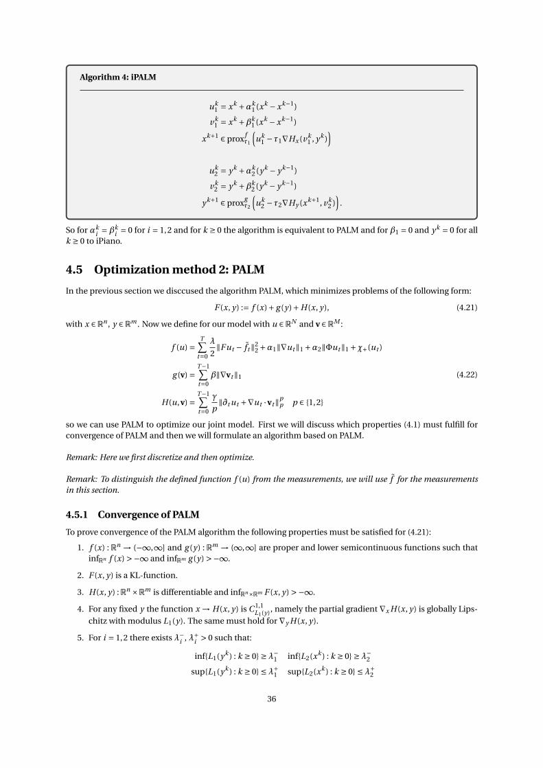
4.5 Optimization method 2: PALM

In the previous section we disccused the algorithm PALM, which minimizes problems of the following form:

F (x, y) := f (x)+ g (y)+H(x, y), (4.21)

with x ∈Rn , y ∈Rm . Now we define for our model with u ∈RN and v ∈RM :

f (u) =T∑

t=0

λ

2‖Fut − ft‖2

2 +α1‖∇ut‖1 +α2‖Φut‖1 +χ+(ut )

g (v) =T−1∑t=0

β‖∇vt‖1

H(u,v) =T−1∑t=0

γ

p‖∂t ut +∇ut ·vt‖p

p p ∈ 1,2

(4.22)

so we can use PALM to optimize our joint model. First we will discuss which properties (4.1) must fulfill forconvergence of PALM and then we will formulate an algorithm based on PALM.

Remark: Here we first discretize and then optimize.

Remark: To distinguish the defined function f (u) from the measurements, we will use f for the measurementsin this section.

4.5.1 Convergence of PALM

To prove convergence of the PALM algorithm the following properties must be satisfied for (4.21):

1. f (x) : Rn → (−∞,∞] and g (y) : Rm → (∞,∞] are proper and lower semicontinuous functions such thatinfRn f (x) >−∞ and infRm g (y) >−∞.

2. F (x, y) is a KL-function.

3. H(x, y) :Rn ×Rm is differentiable and infRn×Rm F (x, y) >−∞.

4. For any fixed y the function x → H(x, y) is C 1,1L1(y), namely the partial gradient ∇x H(x, y) is globally Lips-

chitz with modulus L1(y). The same must hold for ∇y H(x, y).

5. For i = 1,2 there exists λ−i , λ+

i > 0 such that:

infL1(yk ) : k ≥ 0 ≥λ−1 infL2(xk ) : k ≥ 0 ≥λ−

2

supL1(yk ) : k ≥ 0 ≤λ+1 supL2(xk ) : k ≥ 0 ≤λ+

2

36

6. ∇H is Lipschitz continuous on bounded subsets B1 ×B2 of Rn ×Rm . So there exists an M > 0 such thatfor any (xi , yi ) ∈ B1 ×B2 for i = 1,2:∥∥(∇x H(x1, y1)−∇x H(x2, y2),∇y H(x1, y1)−∇y H(x2, y2)

)∥∥≤ M∥∥(x1 −x2, y1 − y2)

∥∥Then the sequence (xk , yk ) ∈Rn ×Rm is generated as follows:

Algorithm 5: PALM

• Initialize: start with x0 and y0 in Rn ×Rm .

• For each k = 1,2, ... generate sequence (xk , yk )k∈N as follows:

1. Take γ1 > 1 and τk1 = γ1

L1(yk ). Compute:

xk+1 = yk −τk1∇x H(xk , yk )

xk+1 ∈ (I +τk1∂ f )−1(xk+1)


L2(xk+1). Compute:

yk+1 = yk −τk2∇y H(xk+1, yk )

yk+1 ∈ (I +τk2∂g )−1(yk+1)

Now we can state the following convergence result from [8].

Theorem 7: Convergence of PALMThe sequence (xk , yk ) for k ∈ N generated by PALM which is assumed to be bounded will convergence to acritical point (x∗, y∗) of F (x, y) if assumptions 1 till 6 are satisfied.

So if we can prove that for (4.1) assumption 1 till 6 hold, then we know that the algorithm will converge to acritical point.

Proof of assumptionsDefine f (u), g (v) and H(u,v) as in (4.22) and choose p = 2 since we need that H(u,v) is a C 1 function.

Assumption 1 and 2By the definition of a norm we have that:

• infRN f (u) = 0,

• infRM g (v) = 0,

• infRN×RM H(u,v) = 0,

so we also have:inf

RN×RMF (u,v) = 0.

The properness and lower semi-continuity of f (u) and g (v) is established in chapter 3 so we have proved as-sumption 1. In chapter 3 we also proved that F (u,v) is a KL function, so we also proved assumption 2.

Assumption 3 and 4In (4.12) and (4.16) we saw that we can rewrite H(u,v) for fixed values of v and u respectively. Next calculatethe partial derivatives of H(u,v) using the definition of the Gâteaux derivative:

d H(u,vk ; u) =⟨γA∗

vk Avk u, u

⟩,

d H(uk ,v; v) =⟨γA∗

uk Auk v, v

⟩.

37

As established in (4.12), (4.15) and (4.16), (4.18), Av and Au are bounded linear operators, hence their adjointsare as well. Now using the boundedness of products of bounded linear maps we can deduce that the givenGatêaux derivatives can be written as bounded and linear operators. This gives us the Fréchet differentiablityof H(u,v), hence we have proved assumption 3.

Now we can define the gradient of H(u, v):

∇u H(u,vk ) = γA∗vk A

vk u,

∇vH(uk ,v) = γA∗uk A

uk v.

For fixed and arbitrary vk calculate:

d(∇u H(u,vk ; u)) =⟨γA∗

vk Avk , u

⟩which is constant and bounded for arbitrary fixed vk , hence the Fréchet derivative of ∇u H(u,vk ) exists forfixed vk and is continuous. So ∇u H(u,vk ) is C 1 and hence L-Lipschitz continuous with constant L1:

L1(vk ) = ‖γA∗vk A

vk ‖2. (4.23)

For fixed and arbitrary uk+1 we get:

d(∇v H(uk+1,v; v)) =⟨γA∗

uk Auk , v

⟩,

so ddv∇v H is also a bounded and constant and hence the derivative exists and is continuous. So ∇v H(uk+1,v)

is L-Lipschitz continuous with constant L2:

L2(uk+1) = ‖γA∗uk A

uk ‖2. (4.24)

So we have proved assumption 4.

Assumption 5Assumption 5 is important, since it guarantees that the step sizes τi for i = 1,2 are well-defined. As mentionedby [8] we can always write:

L′1(vk ) := maxL1(vk ),µ−

1

L′2(uk ) := maxL2(uk ),µ−

2

Note that L′1 and L′

2 are still Lipschitz moduli of ∇u H(·,vk ) and ∇vH(uk , ·). Hence λ−i = µ−

i , with µ−i > 0 for

i = 1,2. Using (4.15) and (4.18), we can write:

λ+1 ≤ γmax |v|2 ·12

λ+2 ≤ γmax |u|2 ·8

(4.25)

with γ> 0, which concludes the proof of assumption 5.

Assumption 6Take any (u1,v1) and (u2,v2) in any bounded subset B1 ×B2 ⊂RN ×RM . Then we can derive:∥∥(

γA∗v1

Av1u1 −γA∗

v2Av2

u2,γA∗u1

Au1v1 −γA∗

u2Au2

v2)∥∥=∥∥(

γ(

A∗v1

Av1u1 − A∗

v2Av2

u1 + A∗v2

Av2u1 − A∗

v2Av2

u2)

,γ(

A∗u1

Au1v1 − A∗

u2Au2

v1 + A∗u2

Au2v1 − A∗

u2Au2

v2))∥∥=

γ2 ∥∥((A∗

v1Av1

− A∗v2

Av2)u1 + A∗

v2Av2

(u1 −u2), (A∗u1

Au1− A∗

u2Au2

)v1 + A∗u2

Au2(v1 −v2)

)∥∥=use that for fixed u, Av is linear in v and for fixed v, Au is linear in u,

γ2 ∥∥(A∗

v1−v2Av1−v2

u1 + A∗v2

Av2(u1 −u2), A∗

u1−u2Au1−u2

v1 + A∗u2

Au2(v1 −v2)

)∥∥≤use assumption 4,

γ2 maxL1(v1 −v2),L2(u1 −u2)‖(u1,v1)‖+maxL1(v2),L2(u2)‖(u1 −u2,v1 −v2)‖ ≤use ‖(u1,v1)‖ ≤C ,

γ2 (maxL1(v1 −v2),L2(u1 −u2))C +max(L1(v2),L2(u2))‖(u1 −u2,v1 −v2)‖so M = γ2 maxL1(v1 −v2),L2(u1 −u2)C +maxL1(v2),L2(u2) > 0, hence we proved assumption 6.

38

4.5.2 PALM for joint reconstruction and motion estimation

We established that (4.1) satisfies all assumptions necessary for the appliction of the PALM algorithm, so thenext step is to formulate the algorithm for joint reconstruction and motion estimation.

Algorithm 6: PALM for joint reconstruction and motion estimation

• Initialize: start with u0 and v0 in RN ×RM .

• For each k = 1,2, ... generate sequence (uk ,vk ) as follows:


L1(vk ). Compute:

uk = uk −τk1∇u H(uk ,vk )

uk+1 = (I +τk1∂ f )−1(uk )


L2(uk+1) . Compute:

vk = vk −τk2∇vH(uk+1,vk )

vk+1 = (I +τk2∂g )−1(vk )

Remark: Since f and g are convex, the proximal map will be single-valued and therefore we can write an equal-ity.

In order to implement the algorithm, we have to make the updates:

uk+1 = (I +τk1∂ f )−1(uk ),

vk+1 = (I +τk2∂g )−1(vk ),

(4.26)

explicit. Where (4.26) corresponds to solving the following minimization problms:

minu

f (u)

minv

g (v).(4.27)

Calculating the proximal map of the whole function f and g is difficult, but since these functions are convexwe can apply a splitting method to simplify this step. Recall from section 4.1 that applying Douglas-Rachfordsplitting is equivalent to iteration using the full proximal step. Employing the equivalence between Douglas-Rachford splitting and ADMM and the equivalence between preconditioned ADMM and PDHG, we use thesteps of PDHG to rewrite (4.26).

As already mentioned in section 4.3, we could rewrite the minimization problems 4.27 to the saddle-pointproblems:

minu

maxp

χ+(u)+⟨K u,p⟩− 1

2λ‖p1‖2

2 −⟨p1, f ⟩−α1δB(L∞)

(p2

α1

)−α2δB(L∞)

(p3

α2

),

minv

maxq

⟨∇v,q⟩−βδB(L∞)

(q

β

)with:

K =F∇Φ

.

Then we obtain algorithm 7 on the next page.

39

Algorithm 7: PALM for joint reconstruction and motion estimation

• Initialize: start with u0 and v0 in RN ×RM .

• For each k = 1,2, ... generate sequence(uk ,vk

)as follows:

1. Take γ1 > 1, τk1 = γ1

L1(vk )and τk

1σk1‖K ‖2 ≤ 1. Compute:

uk+1 =uk −τk1

(γA∗

vk Avk uk

)

uk+1 =

p1k+1 = pk

1 +σk1 F

(uk+1

)pk+1

1 = p1k+1−σk

1 f

λ+σk1

p2k+1 = pk

2 +σk1∇uk+1

pk+12 = min

(α1,max

(−α1, p2k+1

))p3

k+1 = pk3 +σk

1Φ(uk+1

)pk+1

3 = min(α2,max

(−α2, qk+12

))pk+1 = 2pk+1 −pk

uk+1 = uk+1 −τk1

(F∗

(pk+1

1

)−div ·pk+1

2 +Φ∗(pk+1

3

))uk+1 = max

(0, uk+1

)2. Take γ2 > 1, τk

2 = γ2

L2(uk+1)and τk

2σk2‖∇‖2 ≤ 1. Compute:

vk+1 =vk −τk2

(γA∗

uk+1 Auk+1 vk

)

vk+1 =

qk+1 = qk +σk2

(∇ 0

0 ∇

)vk

qk+1 = min(β,max

(−β, q))

vk+1 = vk −τk2

((−div 0

0 −div

)q

)

Parameter choice and stopping criterionTo conclude this section on optimization via PALM we have to set the parameters τk

i , σki and γi for i = 1,2 and

we have to define a stopping criterion.

The stopping criterion follows naturally from the proof of theorem 7, given in [8]. To prove convergence toa critical point they prove that the sequence (uk ,vk ) for k ≥ 0 generated by algorithm 5 is a Cauchy sequence.So the stopping criterion is:

|uk+1 −uk |+ |vk+1 −vk |2|Ω×T | < tol.

Next we will set the parameters. Note that for γi we can pick an arbitrary number greater than one, so thismeans:

τki = γi

1

L ji 6= j

≥ 1

L ji 6= j

for i = 1,2.

40

We also found in (4.25) the following bounds:

L1(vk ) ≤ γmax |vk |2 ·12,

L2(uk ) ≤ γmax |uk |2 ·8,

now we can write:

τk1 ≥ 1

L1(vk )≥ 1

γmax |vk |2 ·12,

τk2 ≥ 1

L2(uk )≥ 1

γmax |uk |2 ·8,

Hence we choose:

τk1 = 1

γmax |vk |2 ·12,

τk2 = 1

γmax |uk |2 ·8.

And for σki we choose:

σk1 = 1

τk1‖K ‖2

σk2 = 1

τk2‖∇‖2

,

= 1

τk1 ·8

= 1

τk2 ·8

,

since ‖∇‖2 ≤ 8, see [15] and for ‖K ‖2 we found:

‖K ‖2 ≤ sup

‖F‖2

‖∇‖2

‖Φ‖2

≤1

81

,

see section 4.3.1.

4.6 Comparison of optimization methods

To get insight about the difference between the two presented optimization methods, we will compare themfor a two dimensional nonconvex optimization problem. Recall from section 3.4.1 the following minimizationproblem:

min(x,y)∈R2

ψ(x, y) = (x y −1)2, (4.28)

note that this function is nonconvex, but convex for fixed x respectively y , this function has the KL-propertyand is C 2. So we can solve this problem by either alternating PDHG or by PALM. This leads to the two algo-rithms on the next page.

For Alternating PDHG to converge, we must have:

τx pk+1 → 0 for k →∞ (4.29)

τy qk+1 → 0, for k →∞

and for PALM we must have:

2τn1 (xn yn −1) → 0 for n →∞ (4.30)

2τn2 (xn+1 yn −1) → 0 for n →∞.

41

Alternating PDHG

• Initialize: start with x1, y1.

• For n = 1,2, ... generate (xn , yn) as fol-lows:

– for k = 1,2, ... generate xn+1 as fol-lows:

– Take τx , σx such that τxσx |yn |2 ≤1

pk+1 = pk +σx yn xk

pk+1 = pk+1−σx1+0.5σx

xk+1 = xk −τx pk+1 yn

xk+1 = 2xk+1 −xk

– while primal-dual gap > tol.

– for k = 1,2, ... generate (yn+1) asfollows:

– Take τy , σy such thatτyσy |xn+1|2 ≤ 1

qk+1 = qk +σy xn+1 yk

qk+1 = qk+1−σy

1+0.5σy

yk+1 = yk −τy qk+1xn+1

yk+1 = 2yk+1 − yk

– while primal-dual gap > tol.

• while

|xn+1 −xn |+ |yn+1 − yn | > tol

PALM

• Initialize: start with x1, y1, take γ1 > 0,γ2 > 0.

• for n = 1,2, ... generate (xn , yn) as fol-lows:

τn1 = γ1

2(yn )2

xn+1 = xn −2τn1 · (xn yn −1)yn

τn2 = γ2

2(xn+1)2

yn+1 = yn −2τn2 · (xn+1 yn −1)xn+1

• while

|xn+1 −xn |+ |yn+1 − yn | > tol

To compare both algorithms we will initialize both algorithms with (x1, y1) = (3,2). We will set the tolerance to10−6. For Alternating PDHG we allow 1000 outer iterations and we will vary the number of inner iterations. ForPALM we will allow also 1000 outer iterations.

It is important to realize that for this simple example we are able to explicitly calculate the values for τx , τy , σx

and σy for Alternating PDHG and τk1 and τk

2 for PALM. However for the more complicated joint reconstructionand motion estimation model we had to estimate upper bounds for these values. We will here investigate howthe quality of this estimation influences the performance of the algorithm.

We will perturb the values of the parameters as follows:

τx =σx = 1

|yn |+δ τn1 = 1

2(yn)2 +δτy =σy = 1

|xn+1|+δ τn2 = 1

2(xn+1)2 +δ .

42

In figure 4.1a one can see how the perturbation δ of the parameters influence the number of iterations neededto converge. We see that for Alternating PDHG the number of iterations grows much fast than for PALM. Wealso see that Alternating PDHG is sensitive for the number of inner iterations. If we choose this number toolow, the subproblems might not converge. This result in a suboptimal approximation for xn+1, which will givea suboptimal solution to the subproblem for yn+1. The result of this can be seen in figure 4.1b, here we onlyallowed 10 inner iterations, which cause Alternating PDHG to ’wander around’ the energy landscape beforeconverging.

(a) Influence of pertubationδ of parameter values on numberof iterations.

(b) Plot of energy for Alternating PDHG (red) with 10 inneriterations and PALM (blue). δ= 8.

Figure 4.1

Finally we plotted the value of (4.29) and (4.30) for each iteration, in figure 4.2a and 4.2b. We see that for PALM,4.30 converges faster and always decreases, which will result in a decrease in energy. For Alternating PDHG,4.29 oscillates more as δ increases. This oscillating will also result in an oscillating energy. This indicates whythe number of iterations grows more when using Alternating PDHG for increasing values of δ.

(a) Convergence plot for τx pk+1 for different values of δ. (b) Convergence plot for 2τn1 (xn yn −1) for different values of

δ.

Figure 4.2

43

Chapter 5

Results and discussion

In this chapter we will present and discuss the results of the joint reconstruction and motion estimation modelfor dynamic MRI. First we will discuss the developed synthetic datasets for dynamic MRI reconstruction andthe used performance measures. Before we can compare both optimization methods we have to define theused subsampling pattern and the motion model for Alternating PDHG. After we defined this, we will use thesynthetic datasets to compare the two optimization methods. After comparison of the two methods we willexplore how the PALM algorithm performs on an experimental medical dataset.

5.1 Datasets & performance measures

A common challenge is that for real experimental medical data no ground truth for the flow field is avaliable.Having a ground truth at hand gives insight in the quality of the motion estimation. To address this we usedthe MPI Sintel dataset [14] used in computer vision to compare motion estimation methods. This dataset hasa ground truth available for the flow field. We will use this dataset to develop a synthetic image sequence fordynamic MRI reconstruction.

We also make use of the 4D XCAT phantom [49] which was made available by the Radiotherapy group of theUMC Utrecht. This 4D phantom is developed for medical imaging research and we will also use this phan-tom to compare the two presented algorithms. Finally the Radiotherapy group of the UMC Utrecht sharedexperimental medical MRI data, which we will use to show the potential of the presented model for real worldscenarios. In the following we will discuss each dataset and its purpose in detail.

5.1.1 Synthetic dataset Hand

The first synthetic dataset is developed using the MPI Sintel dataset. The clean version of the sequence ’Am-bush_7’ was used. We used part of the sequence, were one can see a hand picking up a stick. To create a firsteasy scenario we took the first frame from the sequence and scaled1 the magnitude of the corresponding flowfield. Then we created the second frame by using the discretization of the optical flow constraint:

∂t ut +∇ut ·vt = ut+1 −ut

δt+∇ut ·vt , δt = 1

ut+1 = ut −∇ut ·vt .

Then we used the generated frame to generate the next frame, using the scaled ground truth flow field of thesecond frame. This sequence will satisfy the optical flow constraint, which makes it a good first evaluation.Next the sequence and the ground truth for the flow field are scaled to a size of 256× 256 pixels and trans-formed from RGB to gray values between 0 and 1. In figure 5.1a one can see the whole sequence. The flow fieldcan be seen in figure 5.1c. We will refer to this sequences as the Hand - flow based sequence.

We will also use the original frames of the sequence to create a dataset. Now the image sequence and the flow

1The scaling was chosen such that max |v| < 1, since we have δx = δy = 1 (see appendix B).

44

field will not satisfy the optical flow constraint perfectly, which makes that dataset more challenging. We willrefer to this sequence as the Hand - original sequence, this sequence can be seen in figure 5.1b. The differencein magnitude of the flow field can be seen in figure 5.5b.

(a) Ground truth for the Hand - flow based sequence

(b) Ground truth for the Hand - original sequence

(c) Visualization of the flow field for the Hand-original sequence

Figure 5.1: Ground truth Hand sequences, in the red squares we clearly see the difference between the twodatasets

5.1.2 XCAT 1 & 2

To investigate the influence of both optimization methods on the quality of the reconstruction the XCAT phan-tom [49] is used. This phantom is specially developed for the evaluation of medical reconstruction methods.We extracted two sequences from the 4D phantom. The first sequence shows the heart beating. In the secondsequence a structure will appear over time due to the heartbeat. This results in a source in the flow field, whichis challenging. Both sequences can be seen in figure 5.2.

(a) XCAT sequence 1

(b) XCAT sequence 2

Figure 5.2: Ground truth for the XCAT sequences

45

5.1.3 Experimental medical data

Finally we will use experimental medical data to show the potential of the model for real world scenarios. Thisdata was made available by the radiotherapy group of the UMC Utrecht. The extracted sequence can be seenin figure 5.3.

In this sequence we see a transversal slice of the abdomen. So the back of the person is in the top of theframe. The movement we observe in the sequence is breathing, which is the upward and downward move-ment. We also see the aorta and the inferior vena cava. The aorta transports oxygen ridge blood from the heartto the rest of the body, the inferior vena cava transports oxygenated blood back to the heart. In figure 5.4 wesee a schematic overview of the liver, both veins and the cross-section.

Figure 5.3: Experimental medical data sequence

Figure 5.4: schematic overview of organs visuble in the experimental medical dataset.

5.1.4 Performance measures

To measure the quality of the reconstructed image sequence u and the estimated flow field v we will use thefollowing performance measures.

Peak Signal to Noise Ratio - PSNRThe PSNR is defined as:

PSNR(u,u0) =− log

(‖u −u0‖2

‖u0‖∞

),

were u0 is the ground truth image and u the reconstruction. So the PSNR tells what ratio of the peaks of thesignal is noise.

46

Structural Similarity Index Measure (SSIM)The PSNR is easy to calculate and has a clear physical meaning but it will not reflect visual quality well, there-fore we will also use the SSIM. In [18], [40] and [48] the SSIM is also used to measure the quality of reconstruc-tion so we can compare our results easily.

In [51] the SSIM is defined. The SSIM compares the luminance, contrast and structure of the reconstructedimage u and its ground truth u0. The SSIM is defined as follows:

SSIM(u,u0) = (2µuµu0 + c1)(2σu,u0 + c2)

(µ2u +µ2

u0 + c1)(σ2u +σ2

u0 + c2)

with µ the mean of u and u0 and σ the standard deviation of u and u0. Were c1 and c2 are defined by:[c1 c2

]= [(K1L)2 (K2L)2]

were K1 and K2 are small constants and L the range of the image. We use the implementation of [51] withK = [

0.01 0.03]

and L = 1 since all our images are scaled between [0,1].

Average Endpoint Error - AEEFinally we use the AEE to measure the quality of the estimated flow field v . The AEE is defined in [41] as:

AEE(v,v0) = 1

N

N∑n=1

√(vxn − v0

xn)2 + (vyn − v0

yn)2

with N = nx ny (nt −1).

To also visually inspect the flow fields we will make use of two plots. The first one can be seen in figure 5.5a,were the green arrows indicate the direction of the flow, but are scaled in such a way that the arrows are visible.In 5.5b we can see the magnitude of the flow field, scaled between the maximum and minimum magnitudethat appears in the figure. So magnitude plots with the same figure number, but a different letter have thesame scaling and figures with a different figure numbers have a different scaling.

(a) Plot of the direction of the flow field for the Hand - flow based sequence, note that the flow field of the Hand - originalsequence will have a flow field with a similiar direction.

(b) Plot of the magnitude of the flow field, in the upper row we see the magnitude of the Hand - flow based sequence, in thelower row the magnitude of the Hand - original sequence.

Figure 5.5

47

5.2 Subsampling pattern and motion model

Before we can compare the two optimization methods, we have to define the subsampling pattern and forAlternating PDHG we have to define the motion model.

5.2.1 Subsampling pattern

Now we will define the subsampling pattern P (2.1). As pointed out by [36] random subsampling will result inincoherent artefacts. However this randomness is limited by the fact that in practise the subsampling patternmust be feasable. In section 2.1.2 we briefly discussed subsampling patterns and assumed that we will useCartesian subsampling only. Following [48], Variable density Incoherent Spatio-Temporal Acquistion (VISTA)of [1] is used.

This method is based on minimizing the Riesz energy, which in its simplest form comes down to determiningthe position of N samples such that their mutual distance (in a predefined distance measure) is maximized.However it is desirable to subsample the center of the k-space more, since most of the energy of the imageis concentrated there. This is incorporated in the distance measure, such that sampling the center results inlower costs. An example of a resulting subsampling pattern can be found in figure 5.6.

Figure 5.6: Example of a sequence of six frames with a 6 × subsampled VISTA pattern. So for each frame only16 th of the data remains, which are the white lines. We see that for each frame the subsampling pattern isdifferent.

5.2.2 Choice of motion model

Recall that in the definition of our model we could choose p ∈ 1,2 for the motion model:

M(u,v) = γ

2‖∂t u(·, t )+∇u(·, t ) ·v(·, t )‖p

p .

When using PALM, M(u,v) had to be smooth and hence we choose p = 2. For Alternating PDHG we can useboth p ∈ 1,2. In this section we will compare the result of the motion estimation for both values of p whenusing Alternating PDHG. This comes down to only solving the subproblem for motion estimation in algorithm3 (4.17). We will compare the results for the Hand - flow based sequence, where we take u as the ground truth.β was chosen such that the AEE is minimal.

The AEE of the estimated flow field for the Hand - flow based sequence can be found in table 5.1. The flowfields can be seen in figure 5.7. From both the figure and the table it becomes clear that the model with p = 1performs better. Due to the movement of the hand the shadow also has a changing intensity. It is known thatusing an L1 data-fidelity is more robust to this, as it allows for violations of the optical flow constraint on asparse set, as explained by [3].

So we will use p = 1 in case of optimization via Alternating PDHG. We see that for p = 2 the magnitude ofthe flow field is underestimated, this we will keep in mind when using PALM.

p AEE frame 1 AEE frame 2 AEE frame 3 AEE frame 4 AEE frame 51 0.0190 0.0120 0.0115 0.0109 0.00992 0.2223 0.1881 0.1819 0.1685 0.1547

Table 5.1: AEE of estimated flow field for p = 1,2

48

Result for choice of motion for Alternating PDHG

(a) Ground truth flow field for direction

(b) Ground truth flow field for magnitude

(c) Estimation flow field with p = 1 for direction

(d) Estimation flow field with p = 1 for magnitude

(e) Estimation flow field with p = 2 for direction

(f) Estimation flow field with p = 2 for magnitude

Figure 5.7: Result of motion estimation for p = 1,2

49

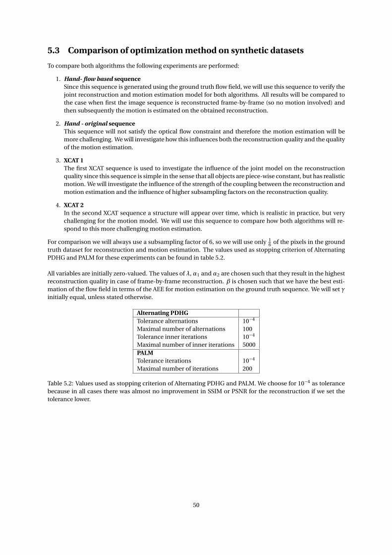
5.3 Comparison of optimization method on synthetic datasets

To compare both algorithms the following experiments are performed:

1. Hand- flow based sequenceSince this sequence is generated using the ground truth flow field, we will use this sequence to verify thejoint reconstruction and motion estimation model for both algorithms. All results will be compared tothe case when first the image sequence is reconstructed frame-by-frame (so no motion involved) andthen subsequently the motion is estimated on the obtained reconstruction.

2. Hand - original sequenceThis sequence will not satisfy the optical flow constraint and therefore the motion estimation will bemore challenging. We will investigate how this influences both the reconstruction quality and the qualityof the motion estimation.

3. XCAT 1The first XCAT sequence is used to investigate the influence of the joint model on the reconstructionquality since this sequence is simple in the sense that all objects are piece-wise constant, but has realisticmotion. We will investigate the influence of the strength of the coupling between the reconstruction andmotion estimation and the influence of higher subsampling factors on the reconstruction quality.

4. XCAT 2In the second XCAT sequence a structure will appear over time, which is realistic in practice, but verychallenging for the motion model. We will use this sequence to compare how both algorithms will re-spond to this more challenging motion estimation.

For comparison we will always use a subsampling factor of 6, so we will use only 16 of the pixels in the ground

truth dataset for reconstruction and motion estimation. The values used as stopping criterion of AlternatingPDHG and PALM for these experiments can be found in table 5.2.

All variables are initially zero-valued. The values of λ, α1 andα2 are chosen such that they result in the highestreconstruction quality in case of frame-by-frame reconstruction. β is chosen such that we have the best esti-mation of the flow field in terms of the AEE for motion estimation on the ground truth sequence. We will set γinitially equal, unless stated otherwise.

Alternating PDHGTolerance alternations 10−4

Maximal number of alternations 100Tolerance inner iterations 10−4

Maximal number of inner iterations 5000PALMTolerance iterations 10−4

Maximal number of iterations 200

Table 5.2: Values used as stopping criterion of Alternating PDHG and PALM. We choose for 10−4 as tolerancebecause in all cases there was almost no improvement in SSIM or PSNR for the reconstruction if we set thetolerance lower.

50

5.3.1 Hand - flow based sequence

The results for the Hand - flow based sequence in terms of the performance measures can be found in table 5.3.We see that for both algorithms, on average and for each frame separately, using a joint model improves boththe reconstruction quality and quality of motion estimation. So using a joint model is as expected beneficial.Using PALM gives even better results, so it is also beneficial to use a nonconvex optimization method.

In table 5.3 we see that the AEE for the flow field of frame 2 estimated via alternating PDHG is much higherthan for the other frames. If we look at this flow field in figure 5.10 (c), we see that the flow fields ’bump intoeach other’. This creates folding, which we can see in figure 5.8. Note that these artefacts do not appear whenusing PALM.

In figures 5.9 and 5.10 the full results are given. From these figures we see that the reconstruction is slightlybetter when using PALM and for the motion estimation we see that PALM underestimates the magnitude ofthe flow. We already observed this underestimation when using p = 2 in section 5.2. This underestimationhowever, still gives lower AEE than the AEE for Alternating PDHG. Which performs better in terms of magni-tude. However the direction of the flow field is often completely wrong (hence the folding), this results in ahigher AEE, despite a better estimation of the magnitude. Here we see that the AEE punishes errors in terms ofdirection more than errors in terms of magnitude.

Measure Algorithm Average Frame 1 Frame 2 Frame 3 Frame 4 Frame 5 Frame 6SSIM only recon. 0.6608 0.2451 0.4886 0.8385 0.8154 0.8033 0.7739

alt. PDHG 0.8409 0.8263 0.8270 0.8571 0.8525 0.8453 0.8371PALM 0.8672 0.8808 0.8780 0.8710 0.8657 0.8586 0.8493

PSNR only recon. 23.75 11.13 13.04 32.64 30.76 29.34 25.59alt. PDHG 33.00 31.55 31.61 34.38 34.10 33.65 32.69PALM 35.02 35.14 35.39 35.41 35.15 34.75 34.28

AEE after recon. 1.1865 1.0651 2.8459 0.4865 0.3644 1.1705alt. PDHG 0.6594 0.3902 1.5007 0.3144 0.2303 0.8614PALM 0.1834 0.2227 0.1887 0.1822 0.1686 0.1549

Table 5.3: Results of joint reconstruction and motion estimation for the ’Hand - flow based’ sequence

(a) Boundary hand and shadow

(b) Boundary hand and sleeve

Figure 5.8: Close up of frame 2 were we can see folding artefacts. Left: ground truth, middle: final reconstruc-tion using alternating PDHG, right: final reconstruction using PALM. We see that this folding does not happenin the reconstruction obtained via PALM.

51

Result of reconstruction for Hand - flow based sequence

(a) Ground truth image sequence

(b) Result for only reconstruction

(c) Result for joint reconstruction and motion estimation via Alternating PDHG

(d) Result reconstruction for joint reconstruction and motion estimation via PALM

Figure 5.9

52

Result of motion estimation for Hand - flow based sequence

(a) Ground truth flow field for direction


(c) Result direction motion estimation for joint reconstruction and motion estimation via Alternating PDHG

(d) Result magnitude motion estimation for joint reconstruction and motion estimation via Alternating PDHG

(e) Result direction motion estimation for joint reconstruction and motion estimation via PALM

(f) Result magnitude motion estimation for joint reconstruction and motion estimation via PALM

Figure 5.10

53

5.3.2 Hand - original sequence

In table 5.4 one can see the results for the Hand- original sequence. Here the motion estimation is more diffi-cult since the motion does not satisfy the optical flow constraint. We see that on average joint reconstructionand motion estimation gives better results. The quality of the motion estimation dropped, which we expectedsince it cannot be explained perfectly by the optical flow constraint. This results also in a lower reconstructionquality. So the model for motion estimation is a limiting factor here. If we now compare both algorithms wesee that for alternating PDHG the reconstruction quality of frames 3,4 and 5 drops in terms of SSIM comparedto frame-by-frame reconstruction. So when the motion estimation becomes more challenging, errors, for ex-ample the folding mentioned earlier, are propagated in the sequence. When using PALM the quality improvesfor each frame compared to frame-by-frame reconstruction. The full results can be found in the appendix(A.1,A.2).


alt. PDHG 0.7971 0.7694 0.7866 0.8161 0.8163 0.8077 0.7866PALM 0.8276 0.8246 0.8369 0.8356 0.8297 0.8257 0.8132


AEE after recon. 2.27 2.4688 3.5035 1.7320 1.4432 2.1865alt. PDHG 1.97 2.1205 2.5730 1.6888 1.4340 2.0121PALM 1.83 2.2264 1.8840 1.8208 1.6868 1.5495

Table 5.4: Results of joint reconstruction and motion estimation for the ’Hand - original’ sequence

5.3.3 XCAT 1 sequence

In table 5.5 we see the results for the first XCAT sequence. Unfortunately we have no ground truth for themotion so we can inspect the flow fields only visually. The flow fields can be seen in figure A.4. We see againa lower magnitude for the flow in the case of using PALM. In the direction plots (a,c) we see that overall thehearts moves in the right direction, so the flow fields do make sense. When using Alternating PDHG we againsee the folding artefacts due to mistakes in the motion estimation. The full result for the reconstruction can befound in figure A.3.

Looking more carefully in table 5.5,we see that the joint reconstruction models outperforms the frame-by-frame reconstruction on average. However for frame 3, we see that frame-by-frame reconstruction gives abetter results than both joint algorithms. This can be explained by the fact that the XCAT sequence consistof piece-wise constant objects, which makes reconstruction easier. The used subsampling pattern for frame3 can now still capture enough information for a good reconstruction. Since there are errors in the motionestimation included and this decreases the quality in this case.

Since the optimization method PALM gives better results we will now investigate for this method the influ-ence of the coupling parameter γ and the influence of the subsampling factor on the reconstruction quality ofthe first XCAT sequence.


alt. PDHG 0.8993 0.8392 0.8633 0.9245 0.9289 0.9265 0.9134PALM 0.9539 0.9523 0.9569 0.9568 0.9554 0.9546 0.9473


Table 5.5: Results of joint reconstruction and motion estimation for the ’XCAT 1’ sequence

54

Influence of coupling γ between reconstruction and motion estimationFor joint reconstruction and motion estimation via PALM we will now investigate the influence of the param-eter γ, which influences the impact of the motion estimation on the reconstruction. The results can be foundin table 5.6.

We see that on average the SSIM is the highest for γ= 0.25, but the PSNR is the highest for γ= 0.5. For γ= 0.1we see the PSNR of the first two frames drop in quality, this are the two frames with the lowest reconstructionquality in the case of frame-by-frame reconstruction and hence we see that a stronger coupling between themotion estimation and reconstruction is needed, since this models the temporal information. For a too strongcoupling of γ = 1.5 however, the reconstruction quality drops as well, since then the flow fields dominate thereconstruction.

γ Measure Average Frame 1 Frame 2 Frame 3 Frame 4 Frame 5 Frame 60.1 SSIM 0.9608 0.9541 0.9653 0.9712 0.9655 0.9595 0.9492

PSNR 30.84 23.03 26.63 35.79 34.47 33.09 32.000.25 SSIM 0.9626 0.9643 0.9666 0.9663 0.9633 0.9615 0.9538

PSNR 33.59 31.20 33.38 35.37 34.62 33.94 33.040.5 SSIM 0.9584 0.9587 0.9620 0.9615 0.9593 0.9583 0.9508

PSNR 33.81 32.81 34.31 34.81 34.25 33.79 32.900.75 SSIM 0.9558 0.9549 0.9591 0.9588 0.9571 0.9563 0.9487

PSNR 33.62 32.68 34.15 34.52 34.05 33.63 32.711 SSIM 0.9539 0.9523 0.9569 0.9568 0.9554 0.9546 0.9473

PSNR 33.44 32.41 33.93 34.35 33.93 33.50 32.531.5 SSIM 0.9494 0.9474 0.9522 0.9526 0.9514 0.9500 0.9429

PSNR 33.03 31.90 33.46 34.01 33.61 33.10 32.08

Table 5.6: Reconstruction quality for different values of γ for the XCAT 1 sequence

Influence of subsampling factorFinally we will investigate the influence of higher subsampling factors on the reconstruction quality. The resultcan be found in table 5.7. First observation is that the joint approach outperforms frame-by-frame reconstruc-tion for all subsampling factors on average. For the joint approach we see that the quality of the reconstructionup to a subsampling factor of 10 is quite good, however from a subsampling of 12 and higher, the quality de-creases.

The reconstruction of frame 5 for each subsampling factor can be seen in figure 5.11 in the case of frame-by-frame reconstruction and in figure 5.12 in the case of joint reconstruction. We see that for R = 12 andR = 14 the joint reconstruction is blurry, but the shapes in the image are better visible than for frame-by-framereconstruction.

4 6 8 10 12 14Frame-by-frame

Average SSIM 0.8675 0.7547 0.6663 0.6161 0.5575 0.5178Average PSNR 29.83 22.79 18.31 16.08 14.99 14.45

JointAverage SSIM 0.9752 0.9584 0.9446 0.9250 0.8348 0.8187Average PSNR 36.59 33.81 32.06 30.49 23.53 23.03

Table 5.7: Average reconstruction quality for different subsampling factors for the XCAT 1 sequence with γ =0.5, compared to frame-by-frame reconstruction.

55

(a) R = 4 (b) R = 6 (c) R = 8

(d) R = 10 (e) R = 12 (f) R = 14

Figure 5.11: Result of frame-by-frame reconstruction of frame 5 for different subsampling factors R.

(a) R = 4 (b) R = 6 (c) R = 8

(d) R = 10 (e) R = 12 (f) R = 14

Figure 5.12: Result of joint reconstruction via PALM of frame 5 for different subsampling factors R

56

5.3.4 XCAT 2 sequence

For this sequence we find results comparable to the results of the XCAT 1 sequence, see table 5.8. In thissequence a structure appears over time. We see in figure 5.13 that for reconstruction using alternating PDHGthis structure is not present but for PALM it is. The full results can be found in the appendix (A.5,A.6).

Figure 5.13: Close up of frame 5 were the structure appeared. Left: ground truth, middle: reconstruction viaalt. PDHG, right: reconstruction via PALM


alt. PDHG 0.9064 0.8554 0.8894 0.9297 0.9317 0.9255 0.9064PALM 0.9639 0.9581 0.9642 0.9643 0.9665 0.9660 0.9643


Table 5.8: Results of joint reconstruction and motion estimation for the XCAT 2 sequence

5.4 Application on experimental medical data

To show the potential of the work presented here we will test the PALM algorithm for joint reconstruction andmotion estimation on the experimental medical data. We will compare the joint reconstruction and motion es-timation model with frame-by-frame reconstruction in terms of the SSIM and PSNR for different subsamplingfactors. In table 5.9 we see that the joint reconstruction performance is better than frame-by-frame recon-struction and the improvement grows as the subsampling factor gets higher.

In figure 5.14b we can see the reconstruction for R = 4. In 5.14c we see the direction of the flow fields. Wesee a clear breathing pattern, first the flow is mainly upwards, during exhalation, then the flow is downward inthe opposite direction during inhalation. Besides the breathing pattern we see also see blood flowing throughboth veins, which creates sources and sink in the flow fields. This is also reflected in figure 5.14d. So our jointmodel also results in a meaningful motion estimation on experimental medical data.

The reconstruction for the other subsampling factors can be found in the appendix, figure A.7 till figure A.10.For R = 8 the motion estimation is given in figure A.11 and figure A.12. Here we still observe the same motionpattern as for R = 4, so for a higher subsampling factor the motion estimation remains meaningful.

R Frame-by-frame Joint4 0.8532 0.90066 0.7142 0.85808 0.6066 0.7904

10 0.5107 0.741712 0.4982 0.7330

R Frame-by-frame Joint4 31.02 33.586 26.53 31.918 24.42 29.69

10 23.08 28.0912 22.92 27.95

Table 5.9: Average SSIM and PSNR for frame-by-frame reconstruction and joint reconstruction for experimen-tal medical data

57

Results for experimental medical sequence for R = 4

(a) Ground truth

(b) Reconstruction for R = 4

(c) Direction of estimated flow field

(d) Magnitude of estimated flow field

Figure 5.14: Results of joint reconstruction and motion estimation for experimental medical data

58

Chapter 6

Conclusion and outlook

Conclusion

To reduce scanning times in dynamic MRI, subsampling of the measurements is needed in practise. With in-creasing subsampling factors, frame-by-frame reconstruction does in general lead to artefacts and insufficientreconstruction quality. Employing information from neighboring frames in time can offer a way to increasethe quality.

To achieve this, we developed a joint reconstruction and motion estimation model for dynamic MRI. Jointlyestimating the motion will result in flow fields which explicitly explain the connection between two frames.The motion estimation is based on the optical flow constraint and the reconstruction uses Compressed Sens-ing as regularization.

We proved the existence of a minimizer, but could not prove uniqueness since the joint model is nonconvex.Due to this nonconvexity the optimization is challenging. In [18], [25] and [35] this is addressed by solving theconvex subproblems for reconstruction and motion estimation in an alternating fashion. However no knowl-edge about the convergence of this approach is known. To address this we developed an algorithm based onthe Proximal Alternating Linearized Minimization (PALM) algorithm [8]. The convergence to a minimum ofthe PALM algorithm relies on the Kurdyka-Lojasiewicz property. We proved that the KL-property holds for thepresented joint model. All other properties that must be satisfied to guarantee the convergence of the PALMalgorithm to a minimum are proved as well.

To compare both optimization methods we also need a ground truth for the flow field. To address the lackof ground truth for medical datasets, we developed a synthetic dataset from datasets used in computer visionfor motion estimation evaluation. These datasets have a ground truth for the flow field available. Combinedwith the XCAT phantom [49], which is specially developed for the evaluation of medical reconstruction meth-ods, we compared both optimization approaches.

In all our experiments we saw that using a joint reconstruction and motion estimation model instead of aframe-by-frame reconstruction enhances the reconstruction quality. We also observed that using PALM as op-timization method gives a higher reconstruction quality than using Alternating PDHG as optimization methodin our cases.

It became clear that the quality of the motion estimation is a limiting factor for the overall quality of the re-construction. We saw that the estimated flow fields reflect the motion in the sequence, but there were somelimitations. In section 5.2.2 we saw that using an L1 data-fidelity resulted in better motion estimation. Sowe used p = 1 for the Alternating PDHG algorithm. However in the case of MRI reconstruction, the motionestimation introduced folding artefacts. When using PALM as optimization method these artefacts were notpresent. For the PALM algorithm we needed p = 2 since we needed to satisfy a smoothness requirement. Wesaw in section 5.2.2 already that using p = 2 resulted in a flow field which underestimated the magnitude ofthe flow, we saw this also in all later experiments.

59

For PALM as optimization method we also explored the influence of the strength of the coupling between thereconstruction and motion estimation on the reconstruction quality. We saw that in case of a very weak cou-pling the reconstruction did not benefit from the temporal information the motion offers, in case of very strongcoupling new artefacts are introduced due to imperfect motion estimation. We also looked at the robustnessfor higher subsampling factors, from which we saw that joint reconstruction is beneficial for all subsamplingfactors. Finally we observed in our cases that PALM is more robust for an appearing structure in the sequenceover time than Alternating PDHG.

To show the potential for real world scenarios, the presented joint model optimized via PALM, was appliedon an experimental medical dataset of a transversal cross-section of the abdomen. The use of the joint modelresulted in higher reconstruction qualities than for a frame-by-frame approach. We also saw that the obtainedflow fields reflected the expected motion in the sequence.

Outlook

To conclude we will evaluate on choices made in this thesis and give suggestions for further research.

Forward operator MRI reconstructionWhen we defined the forward operator for MRI reconstruction we made two assumptions. Firstly, we assumedthat the phase of the received signal by the MRI scanner is negligible small, and hence the resulting image isreal-valued. This assumption is chosen mainly because the motion estimation is defined on real-valued im-ages and since in the joint model the motion is directly incorporated we needed the resulting reconstructedimage to be real-valued as well. However, neglectingnthe complex part of the reconstruction can result in theloss of information which might influence the reconstruction quality. Secondly, we only considered Cartesiansubsampling patterns. However the chosen subsampling pattern has a lot of influence on the artefacts. A goodsuggestion for further research would be to investigate the influence of different types of subsampling pattern(Cartesian, radial, spiral) and what the optimal subsampling patterns would be.

Motion modelAs mentioned before, the used motion model has some limitations. Bu using the PALM algorithm no convex-ity restrictions are imposed on the model. So one possible extension would be to use a non-linear model forthe motion estimation, which could better deal with large displacements. Another suggestion is to make themotion estimation also dependent on all available frames. A possible model extension is given by [9] and [16],were the optical flow is modeled in the field of optimal control. In this model we seek for a flow field, whichexplains the movement in the image sequence over the whole sequence, instead of frame-by-frame. Addi-tionally, in this model we could reconstruct more frames that the number of frames for which we have givenmeasurements. So we could also interpolate.

RegularizationFor both the image sequence u and the flow field v, we made use of simple regularization terms. This choiceallowed us to prove the KL-property and to study the optimization in more detail. Using more advanced reg-ularizers will make the presented optimization more involved, but might improve the results. An interestingextension would be to use the Low-rank plus Sparse decomposition of [40] as regularization for the reconstruc-tion. This decomposition is based on separation of the static background and dynamic foreground. Using thisregularization in a joint reconstruction and motion estimation model might work quite well as the motioncould be estimated only on the sparse dynamic foreground. Then the separation in the low-rank and sparseparts is also motivated by the explicitly modeled motion.

Adding inertiaA straightforward extension for the PALM algorithm is to add an inertia term as mentioned in section 4.4. Thiswill lead to the iPalm algorithm [43]. The inertia term can be seen as an explicit finite difference discretizationof the Heavy-ball with friction dynamical system. Intuitively, adding momentum to the system makes it pos-sible to ’jump’ out of a local minimum and seek for a better minimum in a nonconvex landscape. In [43] theyshow that choosing the right parameters for the initial term gives better results than using no inertial term.

60

Bibliography

[1] R. Ahmad, H. Xue, S. Giri, Y. Ding, J Craft, and O. P. Simonetti. Variable density incoherent spatiotemporalacquisition (VISTA) for highly accelerated cardiac MRI. Magnetic Resonance in Medicine, 74(5):1266–1278,2015.

[2] H. Attouch, J. Bolte, P. Redont, and A. Soubeyran. Proximal Alternating Minimization and ProjectionMethods for Nonconvex Problems: An Approach Based on the Kurdyka-Łojasiewicz Inequality. Mathe-matics of Operations Research, 35(2):438–457, 2010.

[3] G. Aubert, R. Deriche, and P. Kornprobst. Computing Optical Flow via Variational Techniques. SIAMJournal on Applied Mathematics, 60(1):156–182, 1999.

[4] S. Baker, D. Scharstein, J. P. Lewis, S. Roth, M. J. Black, and R Szeliski. A Database and Evaluation Method-ology for Optical Flow. International Journal of Computer Vision, 92:1–31, 2011.

[5] M. Bertero, T.A. Poggio, and V. Torre. Ill-posed problems in early vision. Proceedings of the IEEE, 76(8):869–889, 1988.

[6] J. Bochnak, M. Coste, and M. Roy. Real Algebraic Geometry. Springer Berlin Heidelberg, Berlin, Heidelberg,1998.

[7] J. Bolte, A. Daniilidis, and A. Lewis. The Łojasiewicz Inequality for Nonsmooth Subanalytic Functionswith Applications to Subgradient Dynamical Systems. SIAM Journal on Optimization, 17(4):1205–1223,2007.

[8] J. Bolte, S. Sabach, and M. Teboulle. Proximal alternating linearized minimization for nonconvex andnonsmooth problems. Mathematical Programming, 146(1-2):459–494, 2014.

[9] A. Borzì, K. Ito, and K. Kunisch. Optimal control formulation for determining optical flow. SIAM Journalon Scientific Computing, 24(3):818–847, 2003.

[10] S. Boyd, N. Parikh, E. Chu, and J. Eckstein. Distributed Optimization and Statistical Learning via theAlternating Direction Method of Multipliers. Foundations and Trends R in Machine Learning, 3(1):1–122,2010.

[11] C. Brune. 4D imaging in tomography and optical nanoscopy. Phd thesis, University of Münster, Germany,2010.

[12] M. Burger, H. Dirks, and C. Schönlieb. A Variational Model for Joint Motion Estimation and Image Recon-struction. SIAM Journal on Imaging Sciences, 11(1):94–128, 2016.

[13] M. Burger and S. Osher. A Guide to the TV Zoo. pages 1–70. 2013.

[14] D. J. Butler, J. Wulff, G. B. Stanley, and M. J. Black. A naturalistic open source movie for optical flowevaluation. In European Conf. on Computer Vision (ECCV), pages 611–625, 2012.

[15] A. Chambolle and T. Pock. A first-order primal-dual algorithm for convex problems with applications toimaging. Journal of Mathematical Imaging and Vision, 40(1):120–145, 2011.

[16] K. Chen and D. A. Lorenz. Image sequence interpolation Using Optimal Control. Journal of MathematicalImaging and Vision, 41(1):222–238, 2011.

61

[17] I. Daubechies. Orthonormal Bases of Compactly Supported Wavelets II. Variations on a Theme. SIAMJournal on Mathematical Analysis, 24(2):499–519, 1993.

[18] H. Dirks. Variational Methods for Joint Motion Estimation and Image Reconstruction. PhD thesis, Univer-sity of Münster, Germany, 2015.

[19] D. Donoho, A. Maleki, and M. Sharam. WaveLab. http://statweb.stanford.edu/~wavelab/Wavelab_850/index_wavelab850.html.

[20] A. Dosovitskiy, P. Fischer, E. Ilg, P. Hausser, C. Hazirbas, V. Golkov, P. van der Smagt, D. Cremers, and T. Brox.FlowNet: Learning Optical Flow With Convolutional Networks. In The IEEE International Conference onComputer Vision (ICCV), pages 2758–2766, 2015.

[21] J. Douglas and H. H. Rachford. On the numerical solution of heat conduction problems in two and threespace variables. Transactions of the American Mathematical Society, 82(2):421–421, 1956.

[22] J. Eckstein and D. P. Bertsekas. On the Douglas-Rachford splitting method and the proximal point algo-rithm for maximal monotone operators. Mathematical Programming, 55(1-3):293–318, 1992.

[23] M. J. Ehrhardt and M. M. Betcke. Multi-Contrast MRI Reconstruction with Structure-Guided Total Varia-tion. SIAM Journal on Imaging Sciences, 9(3):1084–1106, 2015.

[24] E. Esser, X. Zhang, and T. F. Chan. A General Framework for a Class of First Order Primal-Dual Algorithmsfor Convex Optimization in Imaging Science. SIAM Journal on Imaging Sciences, 3(4):1015–1046, 2010.

[25] L. Frerking. Variational Methods for Direct and Indirect Tracking in Dynamic Imaging. PhD thesis, Uni-versity of Münster, Germany, 2016.

[26] T. Goldstein, M Li, X. Yuan, E. Esser, and R. Baraniuk. Adaptive Primal-Dual Hybrid Gradient Methods forSaddle-Point Problems. 2013.

[27] Mark A. Griswold, Peter M. Jakob, Robin M. Heidemann, Mathias Nittka, Vladimir Jellus, Jianmin Wang,Berthold Kiefer, and Axel Haase. Generalized Autocalibrating Partially Parallel Acquisitions (GRAPPA).Magnetic Resonance in Medicine, 47(6):1202–1210, 2002.

[28] B. K.P. Horn and B. G. Schunck. Determining Optical Flow. Artificial Inteligence, 17:185–203, 1980.

[29] F. Knoll, K. Bredies, T. Pock, and R. Stollberger. Europe PMC Funders Group Second Order Total General-ized Variation ( TGV ) for MRI. Magnetic Resonance in Medicine, 65(2):480–491, 2014.

[30] Krzysztof Kurdyka. On gradients of functions definable in 0-minimal structures. Annales de l’institutFourier, 1(2):131–295, 1998.

[31] P. L. Lions and B. Mercier. Splitting algorithms for the sum of two nonlinear operators. SIAM Journal ofNumerical Analysis, 16(6):964–979, 1979.

[32] S. Lojasiewicz. Sur la géométrie semi-et sous-analytique. Annales de l’institut Fourier, 43(5):1575–1595,1993.

[33] D. A. Lorenz and T. Pock. An Inertial Forward-Backward Algorithm for Monotone Inclusions. Journal ofMathematical Imaging and Vision, 51(2):311–325, 2015.

[34] B. D. Lucas and T. Kanade. An iterative image registration technique with an application to stereo vision.Proceedings of the 7th International Joint Conference on Artificial Intelligence (IJCAI), 2:674–679, 1981.

[35] F. Lucka, N. Huynh, M. Betcke, E. Zhang, P. Beard, B. Cox, and S. Arridge. Enhancing Compressed Sensing4D Photoacoustic Tomography by Simultaneous Motion Estimation. eprint arXiv:1802.05184, pages 1–29,2018.

[36] M. Lustig, D. Donoho, and J. M. Pauly. Sparse MRI: The application of compressed sensing for rapid MRimaging. Magnetic Resonance in Medicine, 58(6):1182–1195, 2007.

62

http://statweb.stanford.edu/~wavelab/Wavelab_850/index_wavelab850.html

http://statweb.stanford.edu/~wavelab/Wavelab_850/index_wavelab850.html

[37] D. Maurer and A. Bruhn. ProFlow: Learning to Predict Optical Flow. Preprint: arXiv:1806.00800v1, pages1–16, 2018.

[38] M. Menze and A. Geiger. Object scene flow for autonomous vehicles. In Conference on Computer Visionand Pattern Recognition (CVPR), 2015.

[39] P. Ochs, Y. Chen, T. Brox, and T. Pock. iPiano: Inertial Proximal Algorithm for Non-Convex Optimization.SIAM Journal on Imaging Sciences, 7(2):1388–1419, 2014.

[40] R. Otazo, E. Candès, and D. K. Sodickson. Low-rank plus sparse matrix decomposition for accelerateddynamic MRI with separation of background and dynamic components. Magnetic Resonance in Medicine,73(3):1125–1136, 2015.

[41] M. Otte and H. Nagel. Optical flow estimation: Advances and comparisons. In Computer Vision-ECCV’94,pages 49–60. Springer, Berlin, Heidelberg, 1994.

[42] N. Papenberg, A Bruhn, T. Brox, S. Didas, and J. Weickert. Highly Accurate Optic Flow Computation withTheoretically Justified Warping. International Journal of Computer Vision, 67(2):141–158, 2006.

[43] T. Pock and S. Sabach. Inertial Proximal Alternating Linearized Minimization (iPALM) for Nonconvex.SIAM Journal on Imaging Sciences, 9(4):1756–1787, 2016.

[44] M. J.D. Powell. On search directions for minimization algorithms. Mathematical Programming, 4(1):193–201, 1973.

[45] K. P. Pruessmann, M. Weiger, M. B. Scheidegger, and P. Boesiger. SENSE: Sensitivity encoding for fast MRI.Magnetic Resonance in Medicine, 42(5):952–962, 1999.

[46] R.T. Rockafellar. Convex Analysis, pages 32,33,46. 1970.

[47] L. I. Rudin, S. Osher, and E. Fatemi. Nonlinear total variation based noise removal algorithms. Physica D:Nonlinear Phenomena, 60(1-4):259–268, 1992.

[48] M. Schloegl, M. Holler, A. Schwarzl, K. Bredies, and R. Stollberger. Infimal convolution of total generalizedvariation functionals for dynamic MRI. Magnetic Resonance in Medicine, 78(1):142–155, 2017.

[49] W. P. Segars, G. Sturgeon, S. Mendonca, Jason Grimes, and B. M.W. Tsui. 4D XCAT phantom for multi-modality imaging research. Medical Physics, 37(9):4902–4915, 2010.

[50] F. Steinbruecker, T. Pock, and D. Cremers. Large displacement optical flow computation without warping.In Proceedings of the IEEE International Conference on Computer Vision, pages 1609–1614. IEEE, 2009.

[51] Z. Wang, A. C. Bovik, H. R. Sheikh, and E. P. Simoncelli. Image quality assessment: From error visibility tostructural similarity. IEEE Transactions on Image Processing, 13(4):600–612, 2004.

[52] J Weickert and C Schnörr. A theoretical framework for convex regularization in PDE-based computationof image motion. Intl. J. Computer Vision, 45(3):245–264, 2001.

[53] Y. Xu and W. Yin. A Block Coordinate Descent Method for Regularized Multiconvex Optimization withApplications to Nonnegative Tensor Factorization and Completion. SIAM Journal on Imaging Sciences,6(3):1758–1789, 2013.

[54] Y. Xu and W. Yin. A Globally Convergent Algorithm for Nonconvex Optimization Based on Block Coordi-nate Update. Journal of Scientific Computing, 72(2):700–734, 2017.

[55] G. L. Zeng. Medical Image Reconstruction, chapter 10, pages 175–192. 2010.

63

Appendix A

Full results

Result of reconstruction for Hand - original sequence


(b) Result for frame-by-frame reconstruction



Figure A.1

64

Result of motion estimation for Hand - orginal sequence

(a) Ground truth for flow field direction


(c) Result direction motion estimation for joint reconstruction and motion estimation via Alternating PDHG

(d) Result magnitude motion estimation for joint reconstruction and motion estimation via Alternating PDHG

(e) Result direction motion estimation for joint reconstruction and motion estimation via PALM

(f) Result magnitude motion estimation for joint reconstruction and motion estimation via PALM

Figure A.2

65

Result of reconstruction for XCAT 1 sequence


(b) Result for frame-by-frame reconstruction



Figure A.3

66

Result of motion estimation for XCAT 1 sequence

(a) Result direction motion estimation for joint reconstruction and motion estimation via Alternating PDHG

(b) Result magnitude motion estimation for joint reconstruction and motion estimation via Alternating PDHG

(c) Result direction motion estimation for joint reconstruction and motion estimation via PALM

(d) Result magnitude motion estimation for joint reconstruction and motion estimation via PALM

Figure A.4

67

Results for reconstruction of the XCAT 2 sequence


(b) Result for only reconstruction



Figure A.5: Result for ’XCAT 2’ sequence

68

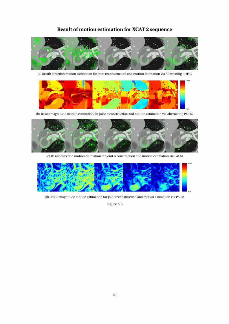
Result of motion estimation for XCAT 2 sequence

(a) Result direction motion estimation for joint reconstruction and motion estimation via Alternating PDHG

(b) Result magnitude motion estimation for joint reconstruction and motion estimation via Alternating PDHG

(c) Result direction motion estimation for joint reconstruction and motion estimation via PALM

(d) Result magnitude motion estimation for joint reconstruction and motion estimation via PALM

Figure A.6

69

Reconstruction of experimental data for R = 6

Figure A.7


Figure A.8


Figure A.9

70


Figure A.10

Result direction motion estimation of experimental data for R = 8

Figure A.11

Result magnitude motion estimation of experimental data for R = 8

Figure A.12

71

Appendix B

Additional definitions and derivations

B.1 Forward difference, central difference and backward difference

Forward differences

∂+t ut =ui , j ,t+1 −ui , j ,t

δt,

∇+x1

ui , j ,t = ui+1, j ,t−ui , j ,t

δxif i > 0 and i < nx

0 if i = 0 or i = nx,

∇+x2

ui , j ,t = ui , j+1,t−ui , j ,t

δyif i > 0 and i < ny

0 if i = 0 or i = ny,

Central differences

∇±x1

ui , j ,t = ui+1, j t ,−ui−1, j ,t

2δxif i > 0 and i < nx

0 if i = 0 or i = nx,

∇+x2

ui , j ,t = ui , j+1,t−ui , j−1,t

2δyif i > 0 and i < ny

0 if i = 0 or i = ny.

Note that central differences is self-adjoint. The adjoint of the forward differences are the backward differ-ences. Hence for the divergence of pi , j ,t =

[pxi , j ,t pyi , j ,t

]we have the following discretization:

Backward differences

div−(pi , j ,t

)=

pxi , j ,t −pxi−1, j ,t

δx1if i > 0 and i < nx

pxi , j ,t

δxif i = 0

− pxi−1, j ,t

δxif i = nx

+

pyi , j ,t −pyi , j−1,t

δyif j > 0 and j < ny

pyi , j ,t

δyif j = 0

− pyi , j−1,t

δyif j = ny

.

Remark: We will set δt = δx = δy = 1.

72

B.2 Convex conjugates

B.2.1 Useful identities

From the definition of the Convex Conjugate of proper functional J : U →R:

J∗(p) := supu∈U

⟨p,u⟩U − J (u)

for p ∈U∗

we can derive:

(J (·+a))∗ = J∗(·)−⟨·, a⟩, (B.1)

(λJ (·))∗ =λJ∗( ·λ

), (B.2)

for λ> 0.

B.2.2 Affine Linear L2 norm

The Convex conjugate of λ2 ‖K u − f ‖2

2 is 12λ‖p‖2

2 +⟨p, f ⟩.

Proof Using Example 2.2.23 of [18] gives that for J (u) = λ2 ‖K u‖2

2 the convex conjugate is J∗(p) = 12λ‖p‖2

2. Com-bining this result with (B.1) we get: (

λ

2‖K u − f ‖2

2

)∗= 1

2λ‖p‖2

2 −⟨p,− f ⟩

= 1

2λ‖p‖2

2 +⟨p, f ⟩.

B.2.3 L1 norm

For J (x) =α‖x‖1 the convex conjugate is J∗(p) =αδB(L∞)(p/α).

Proof Using Example 2.2.4 of [18] we find that for general norm J (x) = ‖x‖χ defined on measurable space χ theconvex conjugate J∗(x∗) = δB(χ∗). Were δB(χ∗) denotes the indicator function of the unit ball in χ∗ defined as:

δB(χ∗)(x∗) =

0 if x∗ ∈ B(χ∗)

∞ else.

Hence we need the dual space of L1 which is L∞. Now employ (B.2), and we obtain:

J∗(p) =αδB(L∞)(p/α).

B.3 Adjoint operators

B.3.1 Adjoint of Fourier transform

Recall that F (·) := P (F (Re(·))). The adjoint operator of the Fourier transform is:

⟨F ( f ), g ⟩ =∫ ∞

−∞F ( f )g (x)dx

=∫ ∞

−∞1

2pπ

∫ ∞

−∞f (t )e−i xt dt g (x)dx

=∫ ∞

−∞f (t )

1

2pπ

∫ ∞

−∞e

¯i xt g (x)dxdt

=∫ ∞

−∞f (t )

1

2pπ

∫ ∞

−∞e−i xt g (x)dxdt

=∫ ∞

−∞f (t )F−1(g (t ))dt

= ⟨ f ,F−1(g )⟩.

73

hence we have proved that for f , g : L2(R2) →R the Fourier transform is a unitary operator, as F∗ =F−1.

The implies:

‖F‖2 = ⟨Fu,Fu⟩= ⟨u,F∗Fu⟩= ⟨u,F−1Fu⟩= ⟨u,u⟩= ‖u‖2.

hence ‖F‖ = 1.

B.3.2 Adjoint of gradient operator

For u, p : L2(Ω) →R, with u of compact support:∫Ω∇u ·pdx =

∫Ω∇· (uv)dx −

∫Ω

u∇·pdx

=∫∂Ω

u ·p ·ndΓ−∫Ω

u∇·pdx

=−∫Ω

u∇·pdx,

using partial integration and the Divergence theorem, the adjoint operator of ∇(·) =−div(·).

B.3.3 Adjoint of wavelet transform

Finally we must determine the adjoint operator for the Wavelet transformΦ(·).

We used the Daubechies wavelet, which is consist of an orthonormal basis and hence is also a unitary op-erator. So the adjoint operator is the inverse of the Daubechies wavelet transform. See [17] for more details.

B.4 Proximal maps

Recall the definition of the proximal map:

x = (I +τ∂T )−1(y),

= prox Tτ (y),

= argminx

‖x − y‖2

2+τT (x)

.

B.4.1 Convex conjugate of affine L2 norm

We have to determine the proximal map of the following functional:

F = 1

2λ‖p‖2

2 +⟨

p, f⟩

,

then we must solve:

proxFσ = arg minp

‖p − p‖2

2

2+σ

(‖p‖2

2

2λ+⟨

p, f⟩)

,

simplify the norm and inner product,

= arg minp

‖p − (p −σ f )‖2

2

2+ σ‖p‖2

2

2λ

.

74

Using the definition of the Gâteaux derivative the mimimum must sastify:

p − (p −σ f )+ σ

λp = 0

p = λ(p −σ f )

λ+σ .

B.4.2 Convex conjugate of L1 norm

We have to determine the proximal map of:

G =αδB(L∞)

( p

α

)=

0 if p ∈ B(L∞)

∞ else.

then we must solve:

proxGσ = arg minp

‖p − p‖2

2

2+σαδB(χ∗)

( p

α

)

If∣∣ pα

∣∣ is greater than α, then δB(L∞)( pα

)=∞, else δB(L∞)( pα

)= 0. So we find that:

p = p

max(α, |p|)is the minimum. In case we have to determine the proximal map of:

G =αδB(L∞)

( p

α

)−⟨

p, f⟩

,

we find:

p = p +σ f

max(α, |p +σ f )|since we can write:

proxGσ = arg minp

‖p − p‖2

2

2+σδB(L∞)

( p

α

)−σ⟨

p, f⟩

= arg minp

‖p − (p +σ f )‖2

2

2+σδB(L∞)

( p

α

).

B.4.3 χ+Finally we need to determine the proximal map of:

H =χ+(ui , j ,t ) :=

0 if ui , j ,t ≥ 0 ∀i , j , t

∞ else,

so we must minimize:

proxHσ = arg minu

‖u − u‖2

2

2+σχ+(u)

.

If u ≥ 0, then u = u will give: proxHσ = 0. If u < 0 then χ+(u) = ∞, so then we choose u = 0 and accept the

difference ‖u − u‖22. Hence we find:

u = max(0, u).

75

joint reconstruction and motion estimation via nonconvex

Documents