john moore slides

8/12/2019 John Moore Slides

http://slidepdf.com/reader/full/john-moore-slides 1/21

A Fast, Parallel Potential Flow Solver

John MooreAdvisor: Jaime Peraire

December 16, 2012

John Moore A Fast, Parallel Potential Flow Solver

http://find/



Outline

1 Introduction to Potential FLow

2 The Boundary Element Method

3 The Fast Multipole Method

4 Discretization

5 Implementation

6 Results

7 Conclusions


http://find/



Why Potential Flow?

It’s easy and potentially fast

Potential Flow: ∇2φ = 0 vs:

Navier-Stokes: ρ∂ V

∂ t

+ V · ∇V = −∇p + ∇ · T + f

Linear system of equations

Full-blown fluid simulation (Navier-Stokes) is expensive

Many times, we are just interested in time-averaged forces,

moments, and pressure distribution.


http://find/

http://goback/



Examples

Start movie 1

1P.O. Persson

Discontinuous Galerkin CFD.Runtime time: > 1 week. 100sof CPUs

Figure 1: Potential Flow Solution.

Runtime time: 2 minutes on 4 CPUs


http://sdles1.avi/

http://sdles1.avi/

http://find/



Potential Flow: Can be Fast, But...

Cannot model everything (highly turbulent flow, etc).

Accuracy issues due linearisation assumptions...

Potential Flow Assumptions

Flow is incompressibleViscosity is neglected (can be a major cause of drag)

Flow is irrotational (∇× V = 0)

But, it turns out to predict aerodynamic flows pretty well formany cases (examples: Flows about ships and aircraft)


http://find/



Potential Flow: Governing Equation

Governed by Laplace’s equation ∇2φ = 0

Potential in domain written as: φ( r ) = φs + φd + V ∞ · r

Enforce that there is no flow in surface-normal direction...Force perturbation potential to vanish just inside the body:

φ( r ) = φs + φd = 0

Basically forces the aerodynamic body to be a streamsurface


http://find/



Potential Flow: Discretization

Can be discretized using the Boundary Element Method (BEM)BEM summary

1 Divide boundary into N elements

2 Analytically integrate Green’s function over each of the N

elements3 Compute the potential due to singularity density at each

element on all other elements

4 Solve for the surface singularity strengths

The BEM requires that either a Neumann or Dirichlet boundarycondition be applied wherever we want a solution.


http://find/



Boundary Element Method: Green’s Function

There are several Green’s functions that satisfy Laplace’sequation:

Singe-Layer potential: G s (σ j , r i − r j ) = 14π

σ j

|| r i − r j ||

Double-Layer potential: G d (µ j , r i − r j ) = 14π

∂

∂ n̂ j

µ j

|| r i − r j ||

φ( r i ) = S j

(G d (µ j , r i − r j ) + G s (σ j , r i − r j )) = 0

These Green’s functions can be analytically integrated toarbitrary precision over planar surfaces

Analytic integral can be very expensive...


C G

http://find/



Boundary Element Method: Collocation vs. Galerkin

Collocation: Enforce boundary condition at N explicit points.

Galerkin: Enforce Boundary condition in an integrated sense overthe surface

1 Write unknown singularity distribution µ as a linearcombination of N basis functions ai

2 Substitute into governing equations, and write a residual

vector R 3 Multiply by test residual by test function.

4 Choose test function to be basis function → residual will beorthogonal to the set of basis functions.

R i = S i ai φi ( r i )dS i =

S i ai

N E j =1

14π

S j µ j

∂

∂ ̂nS j

1

|| r i − r j ||dS j

+ 14π

S j σ j

1|| r i − r j ||

dS j

dSi = 0

(1)John Moore A Fast, Parallel Potential Flow Solver

B d El M h d C i l C id i

http://find/



Boundary Element Method: Computational Considerations

Produces a system that is dense, and may be very large

For example, the aircraft shown earlier would have resulted ina 180000x 180000 dense matrix

Would require 259 GB of memory just to store the systemof equations!

So parallelizing the matrix assembly routine won’t help (yet)

This would be a deal-breaker for large problems, but there is a

solution...


H b id F M l i l M h d (FMM)/ B d El

http://find/



Hybrid Fast Multipole Method (FMM)/ Boundary ElementMethod (BEM)

What is FMM?

A method to compute a fast matrix-vector product (MVP)

Allows MVP to be done in O (p 4N ) operations by sacrificingaccuracy, where p is the multipole expansion order.

We would think that a MVP for a dense matrix scales as

O (N 2

)Theoretically highly parallelizable

More on this later...

FMM can be applied to the BEM

The FMM is easily applied to the Green’s function of Laplace’s Equation

Can think of elements as being composed of many ”source”particles

Maintains same embarrassing parallelism as canonical FMMJohn Moore A Fast, Parallel Potential Flow Solver

FMM St 1 O t d iti

http://find/



FMM Step 1: Octree decomposition

Create “root” box encompassing entire surfaceRecursively divide box until there are no more than N max

elements in a box.Easily Parallizable

Figure 2: All level 8 boxes in octree about an aircraft


FMM St 2 d 3 U d d D d P

http://find/



FMM Steps 2 and 3: Upward and Downward Pass

Basic Idea: Separate near-field and far-field interactions

M →M

M → L

L→ L

Upward Pass

Downard Pass


P ll li ti

http://find/



Parallelization

Four Options:

1 Distributed Memory (MPI)

2 Shared Memory (OpenMP)

3 GPU

4 Julia

Originally, I wrote the FMM code in MATLAB, but was VERYslow

Switched to C++, code sped up 4 orders of magnitude

Now, runtimes are at most several minutes

Weary of scripting due to MATLAB implementation...MPI would be overkill

Ended up computing matrix-vector product in C++ usingOpenMP

System solved in MATLAB using gmres


Implementation

http://find/



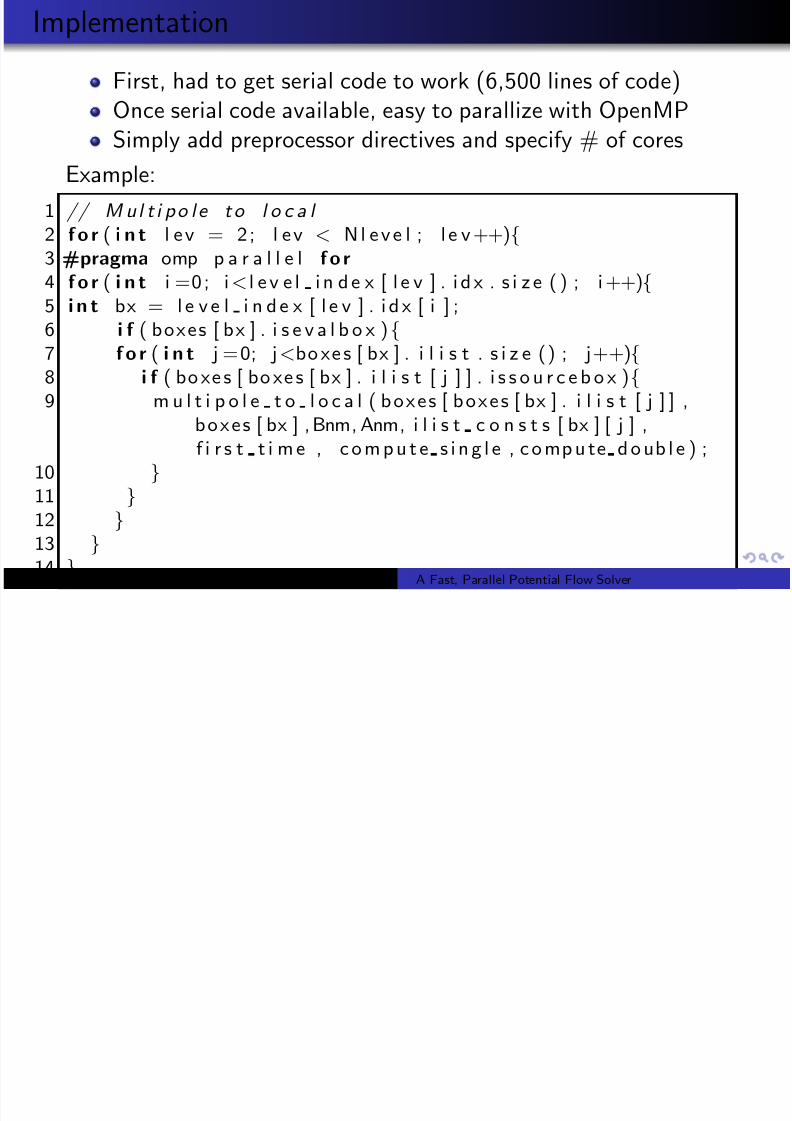
Implementation

First, had to get serial code to work (6,500 lines of code)Once serial code available, easy to parallize with OpenMP

Simply add preprocessor directives and specify # of coresExample:

1 // M u l t i p o l e t o l o c a l 2 f o r ( i n t l e v = 2 ; l e v < N l e v e l ; l e v ++){3 #pragma omp p a r a l l e l f o r

4 f o r ( i n t i =0 ; i< l e v e l i n d e x [ l e v ] . i d x . s i z e ( ) ; i ++){5 i n t bx = l e v e l i n d e x [ l e v ] . i d x [ i ] ;6 i f ( b o x e s [ b x ] . i s e v a l b o x ) {7 f o r ( i n t j = 0; j<bo xe s [ bx ] . i l i s t . s i z e () ; j++){8 i f ( bo xe s [ bo xe s [ bx ] . i l i s t [ j ] ] . i s s o u r c e b o x ) {9 m u l t i p o l e t o l o c a l ( b o x e s [ b o x e s [ bx ] . i l i s t [ j ] ] ,

b o x e s [ bx ] , Bnm, Anm, i l i s t c o n s t s [ bx ] [ j ] ,f i r s t t i m e , c o m p u t e s i n g l e , c o mp u te d o ub l e ) ;

10 }11 }12 }13 }14 }


Solving the System

http://find/



Solving the System

Ax=b solved with GMRES

Matrix is reasonably well-conditioned,but can we do better?

But we never compute the A matrix,

so how do we create a preconditioner?Assemble sparse matrix containingonly near-field interactions.

Then perform ILU on the near-field

influence matrix to createpreconditioner

Figure 3: Near-field influence Matrix


Test Case

http://goforward/

http://find/

http://goback/



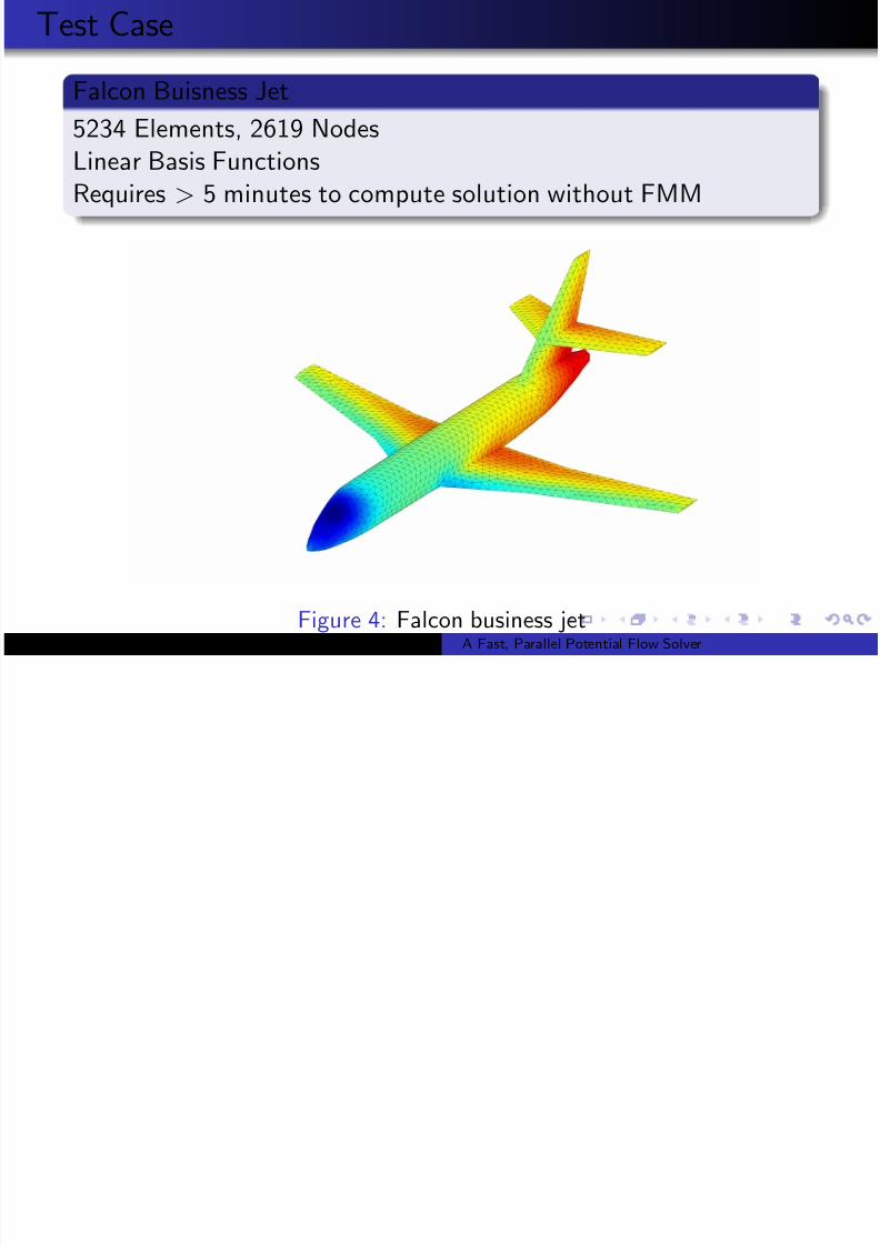
Test Case

Falcon Buisness Jet

5234 Elements, 2619 Nodes

Linear Basis FunctionsRequires > 5 minutes to compute solution without FMM

Figure 4: Falcon business jetJohn Moore A Fast, Parallel Potential Flow Solver

Results

http://find/



Results

Table 1: Speedup compared to 1CPU

p 1 CPU (s) 2 CPUs 3 CPUs 4 CPUs

1 5.2414 1.24 1.36 1.372 8.6618 1.39 1.59 1.703 23.8976 1.65 2.04 2.344 52.4548 1.73 2.26 2.595 105.9322 1.76 2.38 2.79


Conclusions

http://find/



Conclusions

1 C++ is so much faster than MATLAB for BEMs

2 Only really makes sense to use shared memory parallelism (likeOpenMP) for this application

3 Speedups of 2.8X possible on 4 CPUs in some cases

4 Implementation can be improved: this was my first attempt atparallel programming


Thank you for your time!

http://find/



Thank you for your time!

Questions/Comments?


http://find/



Table 2: Percent Speedup

p 1 CPU 2 CPUs 3 CPUs 4 CPUs

1 5.2414 4.2134 3.8450 3.8305

2 8.6618 6.2183 5.4455 5.10493 23.8976 14.5198 11.7185 10.23224 52.4548 30.3419 23.2016 20.25125 105.9322 60.3612 44.4813 37.9687


http://find/

john moore slides

Documents