jit-based cost analysis for dynamic program …eprints.gla.ac.uk/137422/1/137422.pdf ·...

JIT-Based Cost Analysis for Dynamic ProgramTransformations

John Magnus Morton1,4 Patrick Maier2,4 Phil Trinder3,4

School of Computing ScienceUniveristy of Glasgow

UK

Abstract

Tracing JIT compilation generates units of compilation that are easy to analyse and are known to executefrequently. The AJITPar project investigates whether the information in JIT traces can be used to dynam-ically transform programs for a specific parallel architecture. Hence a lightweight cost model is required forJIT traces.This paper presents the design and implementation of a system for extracting JIT trace information from thePycket JIT compiler. We define three increasingly parametric cost models for Pycket traces. We determinethe best weights for the cost model parameters using linear regression. We evaluate the effectiveness of thecost models for predicting the relative costs of transformed programs.

Keywords: Cost Model, JIT Compiler, Program Transformation, Skeleton, Parallelism

1 Introduction

The general purpose hardware landscape is dominated by parallel architectures —multicores, manycores, clusters, etc. Writing performant parallel code is non-trivialfor a fixed architecture, yet it is much harder if the target architecture is not known inadvance, or if the code is meant to be portable across a range of architectures. Exist-ing approaches to address this problem of performance portability, e.g. OpenCL [21],offer device abstraction yet retain a rather low-level programming model typicallyintended for a specific problem domain, e.g. for numerical data-parallel problems.

There is less language support for multiple architectures in other domains. Forexample symbolic computations, like combinatorial searches or computational al-gebra, often exhibit large degrees of parallelism but the parallelism is irregular :

1 Email: [email protected] Email: [email protected] Email: [email protected] This work is funded by UK EPSRC grant AJITPar (EP/L000687/1).

Available online at www.sciencedirect.com

Electronic Notes in Theoretical Computer Science 330 (2016) 5–25

1571-0661/© 2016 Published by Elsevier B.V.

www.elsevier.com/locate/entcs

http://dx.doi.org/10.1016/j.entcs.2016.12.012

This is an open access article under the CC BY-NC-ND license (http://creativecommons.org/licenses/by-nc-nd/4.0/).

mailto:[email protected]



http://www.elsevier.com/locate/entcs



http://www.sciencedirect.com

http://creativecommons.org/licenses/by-nc-nd/4.0/

the number and size of parallel tasks is unpredictable, and parallel tasks are oftencreated dynamically and at high rates [28].

The Adaptive Just-in-Time Parallelism (AJITPar) project [2] investigates a novelapproach to deliver portable parallel performance for programs with irregular paral-lelism across a range of architectures by combining declarative task parallelism withdynamic scheduling and dynamic program transformation. Specifically, AJITParproposes to adapt task granularity to suit the architecture by transforming tasks atruntime, thus varying the amount of parallelism depending on the architecture. Tofacilitate dynamic transformations, AJITPar will leverage the dynamic features ofthe Racket language and its recent trace-based JIT compiler, Pycket [13,10].

Dynamic task scheduling and task transformation both benefit from predictedtask runtimes. This paper investigates how to construct lightweight cost models forJIT traces. A JIT trace is simply a linear path through the program control flowgraph that the compiler has identified as being executed often. We hypothesize thateven very simple cost models can yield sufficiently accurate predictions as traceshave very restricted control flow, and we only require to compare the relative costsof pre- and post-transformed expressions.

The main contributions in this paper are as follows. We have designed and imple-mented a system for extracting JIT trace information from the Pycket JIT compiler(Section 3). We have defined 3 cost models for JIT traces, ranging from very simpleto parametric, and we have used an regression analysis over the Pycket benchmarksuite to automatically tune the architecture-specific cost model parameters (Sec-tion 4). We have shown that the tuned cost model can be used to accurately predictthe relative execution times of transformed programs (Section 5).

2 Related Work

2.1 AJITPar

The Adaptive Just-In-Time Parallelisation (AJITPar) project [2] aims to investigatea novel approach to deliver portable parallel performance for programs with irreg-ular parallelism across a range of architectures. The approach proposed combinesdeclarative parallelism with Just In Time (JIT) compilation, dynamic scheduling,and dynamic transformation. The project aims to investigate the performance porta-bility potential of an Adaptive Skeletons (AS) library based on task graphs, and anassociated parallel execution framework that dynamically schedules and adaptivelytransforms the task graphs. We express common patterns of parallelism as a rel-atively standard set of algorithmic skeletons [17], with associated transformations.Dynamic transformations, in particular, rely on the ability to dynamically compilecode, which is the primary reason for basing the framework on a JIT compiler.Moreover, a trace-based JIT compiler can deliver estimates of task granularity bydynamic profiling and/or dynamic trace cost analysis, and these can be exploitedby the dynamic scheduler. A trace-based JIT-compiled functional language waschosen as functional programs are easy to transform; dynamic compilation allowsa wider range of transformations including ones depending on runtime information;

J.M. Morton et al. / Electronic Notes in Theoretical Computer Science 330 (2016) 5–256

and trace-based JIT compilers build intermediate data structure (traces) that maybe costed.

The work described in this paper aims to identify a system for calculating relativecosts of traces, which will be used to determine the scheduling of parallel tasks basedon their relative costs, and the selection of appropriate transformations to optimisefor the parallel work available in the task.

2.2 Tracing JIT

Interpreter-based language implementations, where a program is executed upon avirtual machine rather than on a real processor are often used for a variety of reasons- including ease of use, dynamic behaviour and program portability, but are oftenknown for their poor performance compared to statically compiled languages suchas C or FORTRAN.

JIT compilation is a technology that allows interpreted languages to significantlyincrease their performance, by dynamically compiling well-used parts of the pro-gram to machine code. This enables interpreters or virtual machine languages toapproach performance levels reached by statically compiled programs without sac-rificing portability. Dynamic compilation also allows optimisations to be performedwhich might not be available statically.

JIT compilation does not compile the entire program as it is executed, rather itcompiles small parts of the program which are executed frequently (these parts aredescribed as hot). The most common compilation units are functions (or methods)and traces [8]. A trace consists of a linear sequence of instructions which make upa single iteration of the body of loop. A complete trace contains no control-flowexcept at the points where execution could leave the trace; these points are knownas guards. The main benefit of traces compared to functions as a unit of compilationis that it can form the entire body of a loop spanning multiple functions, rather thanjust the body of a single function.

2.3 RPython Tool-chain

The specific JIT technology we use is part of the RPython tool-chain. PyPy [32] isan alternative implementation of the Python programming language [33], notable forhaving Python as its implementation language. PyPy is implemented using a subsetof the Python language known as RPython and the tool-chain is intended to beused as a general compiler tool-chain. Smalltalk [12] and Ruby [39] are examples oflanguages implemented on the RPython tool-chain. PyPy has a trace-base JIT, andthe RPython tool-chain allows for the JIT to be easily added to a new interpreterimplementation

Pycket [13] is an implementation of the Racket language built on PyPy’s tool-chain. Racket is a derivative of the Scheme Lisp derivative [37] with a number ofextra features. Pycket uses the Racket front-end to compile a subset of Racket toa JavaScript Object Notation (JSON) representation of the abstract syntax tree(AST) and uses an interpreter built with the RPython tool-chain to interpret the

J.M. Morton et al. / Electronic Notes in Theoretical Computer Science 330 (2016) 5–25 7

AST.JITs built with RPython are notable in that they are meta-tracing [11]. Rather

than trace an application level loop, the JIT traces the actual interpreter loop itself.The interpreter will annotate instructions where an application loop begins and endsin order for appropriate optimisations to be carried out. The purpose of this is sothat compiler writers do not need to write a new JIT for every new language thattargets RPython/PyPy, they just provide annotations.

2.4 Cost Analysis

Resource analysis is important in resource-limited systems like most embedded sys-tems, in hard real-time systems where timing guarantees are required, and for direct-ing program refactoring or transformation. Here we seek a static resource analysisto inform dynamic program transformations. Recently there has been significantprogress in both the theory and practice of resource analysis. Some of this progessis reported in the FOPARA workshops [19] and the TACLe EU COST action [38].

Analysis techniques exist for a range of program resources, for example executiontime [41,1,34], space usage [36,26], or energy [22]. The resource of interest hereis predicted execution time. For many applications, e.g. embedded and real-timesoftware systems, the most important performance metric is worst case executiontime. Various tools [41,20,1] have been built to statically estimate or measure this;an example is aiT [20] which uses a combination of control flow analysis and lowerlevel tools, such as cache and pipelining analysis. Cache and pipelining analysisattempts to predict the caching and processor pipelining behaviour of a programand is performed in aiT using abstract interpretation. Here however we predictexpected, rather than worst case execution time. Moreover we do not need preciseabsolute costs: approximate relative costs should suffice to allow the transformationengine to select between alternative rewrites.

A range of analysis techniques are used to estimate the resources used by pro-grams. High level cost analysis can be performed on the syntactic structure ofthe source code of a program, e.g. using a mathematical function of C syntacticconstructs to estimate execution time [15]. Low-level representations of code andbytecode can be used as source for static resource analysis [3,4,26,7,6]. For examplethe COSTA tool [4] for Java which allows the analysis of various resources usingparameterized cost models, and the CHAMELEON tool [7] which builds on thisapproach and uses it to adapt programs.

There are many other approaches in cost analysis including amortized resourceanalysis [23,6], incremental resource analysis [5], and attempting to enforce resourceguarantees using proof-carrying code [6,9] (the MOBIUS project is a prime example).

Control flow is a key element of many resource analyses [41,20]. However, as JITtraces do not contain any control flow, these types of analysis are redundant and afar simpler approach will suffice. This is fortunate as the static analysis must runfast as part of the warm-up phase of the execution of the JIT compiled program.

Our work is part of the body of work that applies resource analysis to paral-lelism [40,3,34].


2.5 Code Transformation

Program transformations are central to optimising compilers. GHC, for instance,aggressively optimises Haskell code by equational rewriting [24,25]. Transformationscan also be used for optimising for parallel performance. Algorithmic skeletons [17]– high level parallel abstractions or design patterns – can be tuned by code trans-formations to best exploit the structure of input data or to optimise for a particularhardware architecture. Examples of this include the PMLS compiler [35], whichtunes parallel ML code by transforming skeletons based on offline profiling data,and the Paraphrase Project’s refactorings [16] and their PARTE tool for refactoringparallel Erlang programs [14]. PMLS is an automatically parallelising compiler forStandard ML which turns nested sequential higher-order-function calls into parallelskeleton calls and performs code transformation based on runtime behaviour of sub-parts of the program; unlike AJITPar, these transformations are entirely offline andno attempt is made to solve the problem of performance portability. PARTE usesrefactoring to allow the introduction of parallel skeletons and the transformationof existing parallel skeletons; these refactorings are applied entirely ahead-of-timeand at the instruction of the user, while the transformations are driven by offlineprofiling.

3 Language Infrastructure

3.1 Pycket Trace Structure

A JIT trace consists of a series of instructions recorded by the interpreter, and atrace becomes hot if the number of jumps back to the start of the trace (or loop) ishigher than a given threshold, indicating that the trace may be executed frequentlyand is worth compiling.

Other important concepts in Pycket traces include guards : assertions which causeexecution to leave the trace when they fail; bridges : that are traces starting at aguard that fails often enough; and trace graphs : representing sets of traces. Thenodes of a trace graph are entry points (of loops or bridges), labels, guards, andjump instructions. The edges of a trace graph are directed and indicate controlflow. Note that control flow can diverge only at guards and merge only at labels orentry points. A trace fragment is a part of a trace starting at a label and endingat a jump, at a guard with a bridge attached, or at another label, with no label inbetween.

The listing in Figure 1 shows a Racket program incrementing an accumulatorin a doubly nested loop, executing the outer loop 105 times and the inner loop 105

times for each iteration of the outer loop, thus counting to 1010.Figure 1 also shows the trace graph produced by Pycket. The nodes represent

instructions which are pertinent to the flow of control through the loop. In thegraph, labels are represented by l nodes, g nodes represent guards and j nodesrepresent jump instructions. The inner loop (which becomes hot first) correspondsto the path from l2 to j1, and the outer loop corresponds to the bridge. The JIT


( d e f i n e numb1 100000)( d e f i n e numb2 100000)

( d e f i n e ( inner i t e r acc )( i f (> i t e r numb2)

acc( inne r (+ i t e r 1) (+ acc 1 ) ) ) )

( d e f i n e ( outer i t e r acc )( i f (> i t e r numb1)

acc( outer (+ i t e r 1) ( inne r 0 acc ) ) ) )

( outer 0 0)

Loop Entry

l1

l2

g1

g2

g3

j1

Bridge Entry b2

l3

j2

Fig. 1. Doubly nested loop in Racket and corresponding Pycket trace graph.

l a b e l ( i7 , i13 , p1 , de sc r=TargetToken (4321534144))debug_merge_point (0 , 0 , ’ ( l e t ( [ i f_0 (> i t e r numb2 ) ] ) . . . ) ’ )guard_not_inval idated ( desc r=<Guard0x10196a1e0>) [ i13 , i7 , p1 ]debug_merge_point (0 , 0 , ’(> i t e r numb2 ) ’ )i 14 = int_gt ( i7 , 100000)guard_fa l se ( i14 , de sc r=<Guard0x10196a170>) [ i13 , i7 , p1 ]debug_merge_point (0 , 0 , ’ ( i f i f_0 acc . . . ) ’ )debug_merge_point (0 , 0 , ’ ( l e t ( [ AppRand0_0 . . . ] . . . ) . . . ) ’ )debug_merge_point (0 , 0 , ’(+ i t e r 1 ) ’ )i 15 = int_add ( i7 , 1)debug_merge_point (0 , 0 , ’(+ acc 1 ) ’ )i 16 = int_add_ovf ( i13 , 1)guard_no_overflow ( desc r=<Guard0x10196a100>) [ i16 , i15 , i13 , i7 , p1 ]debug_merge_point (0 , 0 , ’ ( inne r AppRand0_0 AppRand1_0 ) ’ )debug_merge_point (0 , 0 , ’ ( l e t ( [ i f_0 (> i t e r numb2 ) ] ) . . . ) ’ )jump( i15 , i16 , p1 , de sc r=TargetToken (4321534144))

Fig. 2. Trace fragment l2 to j1.

compiler unrolls loops once to optimise loop invariant code, producing the path froml1 to l2.

The trace graph is a convenient representation to read off the trace fragments.In this example, there are the following four fragments: l1 to l2, l2 to g2, l2 to j1,and l3 to j2. Trace fragments can overlap: for instance, l2 to j1 overlaps l2 to g2.

Figure 2 shows a sample trace fragment, l2 to j1, corresponding to the inner loop.Besides debug instructions, the fragment consists of 3 arithmetic-logical instructionsand 3 guards (only the second of which fails often enough to have a bridge attached).

The label at the start brings into scope 3 variables: the loop counter i7, theaccumulator i13, and a pointer p1 (which plays no role in this fragment). The jumpat the end transfers control back to the start and also copies the updated loopcounter and accumulator i15 and i16 to i7 and i13, respectively.


3.2 Runtime Access to Traces and Counters

The RPython tool chain provides language developers with a rich set of APIs tointeract with their generic JIT engine. Among these APIs are a number of call-backs that can intercept intermediate representations of a trace, either straight afterrecording, or after optimisation. We use the latter callback to obtain the optimisedtrace for cost analysis.

In debug mode RPython can instrument traces with counters, recording howoften control reaches an entry point or label. RPython provides means to inspectthe values of these counters at runtime. AJITPar will use this feature in the futureto derive estimates of the cost of whole loop nests from the cost and frequency oftheir constituent trace fragments. For now, we dump the counters as the programterminates and use this information to evaluate the accuracy of trace cost analysis(Section 4).

The JIT compiler counts the number of times a label is reached but we are moreinterested in counting the execution of traces. Unfortunately, full traces as gatheredby our system cannot be simply counted, as guards can fail and jumps can targetany label. Fortunately, we can work out the trace fragment execution count due tothe fact that there is a one-to-one correspondence between guards and their bridges.Essentially, the frequency of a fragment � to g is the frequency of the bridge attachedto guard g. Trace fragments are the largest discrete part of traces we can accuratelycount. The frequency of a fragment starting at � and not ending in a guard is thefrequency of label � minus the frequency of all shorter trace fragments starting at�. Table 1 and Table 2 demonstrate this on the trace fragments of the nested loopexample. The first two columns show the JIT counters, the remaining three columnsshow the frequency of the four trace fragments, and how they are derived from thecounters. Note that not all counters reach the values one would expect from theloop bounds. This is because counting only starts once code has been compiled;iterations in warm-up phase of the JIT compiler are lost. The hotness threshold iscurrently 131 for loops.

JIT counter JIT countnl1 100,001nl2 10,000,098,957nb2 99,801nl3 99,800

Table 1JIT counters and counts for program in Figure 1.

3.3 JIT Instruction Classes

When discussing the cost models, it is useful to classify the RPython JIT instructionsinto different sets. We begin with the set of all instructions all. Initially, it wasdecided to sub-divide all into two subsets: the set debug instructions debug and all


fragment frequency expression frequencyl1 to l2 nl1 100,001l2 to g2 nb2 99,801l2 to j1 nl2 − nb2 9,999,999,156l3 to j2 nl3 99,800

Table 2JIT counters and trace fragment frequencies for program in Figure 1.

other instructions; this is based on the idea that debug operations are removed byoptimisations and do not count towards runtime execution costs.

It was further theorised that some instructions will be more costly than oth-ers. The set of all non-debug instructions was further subdivided into high-costinstructions high and low-cost instructions low, based on their expected relativeperformance.

Class Example Instructionsdebug debug_merge_point

numeric int_add_ovfguards guard_truealloc new_with_vtablearray arraylen_gcobject getfield_gc

Table 3RPython JIT Instruction Classes

Further classification of the instructions can be made based on the conceptualgrouping of them and makes no assumptions of their performance characteristics.The classes are object read and write instructions object, guards guards, numericalinstructions numeric, memory allocation instructions alloc and array instructionsarray. These classes are described in Table 3. Jump instructions are ignored, sincethere is only ever one in a trace. External calls are excluded as two foreign functioncalls could do radically different things.

A histogram of JIT operations, taken from traces generated by all the cross-implementation benchmarks and shown in Figure 3, shows that overall these tracesare also dominated by instructions from the guards, objects and numeric classes.

4 JIT-based Cost Models

The traces produced by Pycket during JIT compilation provide excellent informationfor cost analysis. The linear control flow makes traces easy to analyse, and the factthat traces are only generated for sufficiently “hot” code focuses cost analysis on themost frequently executed code paths. In this section, we define several cost modelsbased on trace information collected from Pycket.


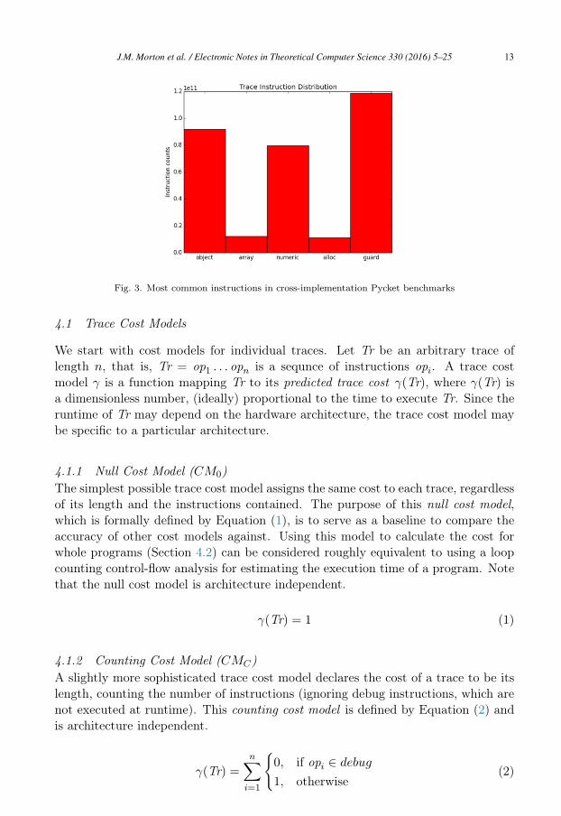
Fig. 3. Most common instructions in cross-implementation Pycket benchmarks

4.1 Trace Cost Models

We start with cost models for individual traces. Let Tr be an arbitrary trace oflength n, that is, Tr = op1 . . . opn is a sequnce of instructions opi. A trace costmodel γ is a function mapping Tr to its predicted trace cost γ(Tr), where γ(Tr) isa dimensionless number, (ideally) proportional to the time to execute Tr. Since theruntime of Tr may depend on the hardware architecture, the trace cost model maybe specific to a particular architecture.

4.1.1 Null Cost Model (CM0)The simplest possible trace cost model assigns the same cost to each trace, regardlessof its length and the instructions contained. The purpose of this null cost model,which is formally defined by Equation (1), is to serve as a baseline to compare theaccuracy of other cost models against. Using this model to calculate the cost forwhole programs (Section 4.2) can be considered roughly equivalent to using a loopcounting control-flow analysis for estimating the execution time of a program. Notethat the null cost model is architecture independent.

γ(Tr) = 1 (1)

4.1.2 Counting Cost Model (CMC)A slightly more sophisticated trace cost model declares the cost of a trace to be itslength, counting the number of instructions (ignoring debug instructions, which arenot executed at runtime). This counting cost model is defined by Equation (2) andis architecture independent.

γ(Tr) =n∑

i=1

{0, if opi ∈ debug

1, otherwise(2)


4.1.3 Weighted Cost Model (CMW )Certain types of instructions are likely to have greater execution time, for examplememory accesses may be orders of magnitude slower than register accesses. A moreintricate cost model can be obtained by applying a weighting factor to each of theinstruction classes described in Section 3.3. Equation (3) shows the definition of thisweighted cost model, parameterised by abstract weights a, b, c, d and e.

γ(Tr) =n∑

i=1

⎧⎪⎪⎪⎪⎪⎪⎪⎪⎪⎨⎪⎪⎪⎪⎪⎪⎪⎪⎪⎩

0, if opi ∈ debug

a, if opi ∈ array

b, if opi ∈ numeric

c, if opi ∈ alloc

d, if opi ∈ guard

e, if opi ∈ object

(3)

The accuracy of the model depends on the concrete weights, and their choice dependson the actual architecture. Section 4.3 demonstrates how to obtain concrete weightsfor a reasonably accurate model.

4.2 Whole Program Cost Models

Let P be a program. During an execution of P , the JIT compiler generates m

distinct traces Trj and m associated trace counters nj .Given a (null, counting or weighted) trace cost model γ, we define the (null,

counting or weighted) cost Γ(P ) of P by summing up the cost of all traces, eachweighted by their execution frequency; see Equation (4) for a formal definition.

Γ(P ) =m∑j=1

nj γ(Trj) (4)

Note that Γ is not a predictive cost model, as its definition relies on traces and tracecounters, and the latter are only available after the execution of a program. However,Γ can still be useful for predicting the cost of transformations, as demonstrated inSection 5.

4.3 Calibrating Weights for CMW

To use the abstract weighted cost model CMW (Section 4.1.3), it is necessary to findconcrete values for the weight parameters a, . . . , e in Equation (3). Ideally, programcost Γ(P ) is proportional to program runtime t(P ). That is, ideally there existsk > 0 such that Equation (5) holds for all programs P .

Γ(P ) = k t(P ) (5)

Given sufficiently many programs, we can use Equation (5) to calibrate the weightsof CMW for a given architecture by linear regression, as detailed in Section 4.3.2.


4.3.1 BenchmarksFor the purpose of calibrating weights we use 41 programs from the standard Pycketbenchmark suite pycket-bench [31] and the Racket Programming Languages Bench-mark Game suite [18]. The programs used are a subset of the full suite, as programsthat result in failing benchmark runs or which contain calls to foreign functions areomitted. Foreign function calls are removed as it is unlikely that any two foreignfunction calls are doing the same thing or take the same time.

For each program, we record the execution time, averaging over 10 runs. Wealso record all traces and the values of all trace counters; since all benchmarks aredeterministic traces and trace counters do not vary between runs.

The Pycket version used for these experiments is revision e56ba66d71 of thetrace-analysis branch of our custom fork [29], built with Racket version 6.1 andrevision 79009 of the RPython toolchain. The experiments are run on a 16 core 2.0GHz Xeon server with 64 GB of RAM running Ubuntu 14.04.

4.3.2 Linear RegressionPicking an arbitrary value for k, e.g. k = 1, we derive the following relation fromEquations (5) and (4).

t(Pl) = Γ(Pl) + εl =

ml∑j=1

nlj γ(Trlj) + εl (6)

Pl is the lth benchmark program, generating ml traces Trlj and trace counters nlj ,t(Pl) is the observed average runtime of Pl, and εl is the error term. Equation (6)becomes a model for linear regression by expanding γ according to its definition(3), which turns the right-hand side into an expression linear in the five unknownweights a, . . . , e.

Weights are implicitly constrained to be non-negative, as negative weights wouldsuggest that corresponding instructions take negative time to execute, which is phys-ically impossible. To honour the non-negativity constraint, weights are estimatedby non-negative least squares linear regression.

γ(Tr) =k∑

i=1

⎧⎪⎪⎪⎪⎨⎪⎪⎪⎪⎩

4.884× 10−4, if opi ∈ numeric

4.797× 10−3, if opi ∈ alloc

4.623× 10−4, if opi ∈ guard

0, otherwise

(7)

Equation (7) shows the resulting weighted cost model for the Xeon server architec-ture. This model only attributes non-zero cost to allocation, numeric instructionsand guards, implying that object and array access instructions have negligible cost.

The regression fit for this cost model is shown in Figure 4. The fit is obviouslylinear but rather coarse, indicating that CMW is not a very accurate model. There isone egregious outlier (the trav2 benchmark – a tree traversal program); a possibleexplanation is that the program is spending most of its time in the interpreter


Fig. 4. Execution time vs cost for CMW determined using linear regression

rather than compiled code, resulting in an underestimation of cost due to lack oftrace output to measure. We note that linear regression fits for CMC and CM0 arevisibly worse than the fit for CMW , which implies that their accuracy is lower thanCMW .

5 Costing Transformations

The main purpose of a cost model in the AJITPar project is to enable the selec-tion and parameterisation of appropriate dynamic transformations. This sectionidentifies the transforms and explores how accurately the cost models predict theexecution time of programs before and after transformation.

5.1 Skeleton Transforms

In AJITPar parallel programs are expressed by composing algorithmic skeletons [17]from an Adaptive Skeletons (AS) library [27].

Adaptive skeletons are based on a standard set of algorithmic skeletons for spec-ifying task-based parallelism within Racket. The AS framework expands skeletonsto task graphs and schedules tasks to workers; expansion and scheduling happen atruntime to support tasks with irregular granularity. The AS framework piggy-backson Pycket to analyze the cost of tasks as they are executed. The cost informationis used both to guide the dynamic task scheduler as well as a skeleton transfor-mation engine. The latter adapts the task granularity of the running program tosuit the current architecture by rewriting skeletons according to a standard set ofequations [27].

A number of different skeleton types are used in AJITPar. The basic typesof skeletons are parallel map, parallel reduce and divide and conquer. The actualversions of the skeletons in AJITPar are tuneable, in that they are parameterisedwith a number that specifies the granularity of the parallelism in some way. Thedefinitions of some of these tuneable skeletons, parMapChunk, parMapStride and


−− map s k e l e t on sparMap : : ( a → b) → [ a ] → [ b ]parMap f [ ] = [ ]parMap f ( x : xs ) = spawn f x : parMap f xs

parMapChunk : : In t → ( a → b) → [ a ] → [ b ]parMapChunk k f xs = concat $ parMap (map f ) $ chunk k xs

parMapStride : : Int → ( a → b) → [ a ] → [ b ]parMapStride k f xs = concat $ transpose $ parMap (map f )

$ transpose $ chunk k xs

−− d i v i d e and conquer s k e l e t on sparDivconq : : ( a → [ a ] ) → ( [ b ] → b) → ( a → b) → a → bparDivconq div comb conq x =

case div x o f[ ] → spawn conq xys → spawn comb (map (parDivconq div comb conq ) ys )

parDivconqThresh : : ( a → Bool ) → ( a → [ a ] ) → ( [ b ] → b)→ ( a → b) → a → b

parDivconqThresh thresh div comb conq x= i f thresh x

then spawn (divconq div comb conq ) xe l s e case div x o f

[ ] → spawn conq xys → comb (map (parDivconqThresh p div comb conq ) ys )

−− s i gna tu r e s o f a u x i l i a r y func t i onschunk : : Int → [ a ] → [ [ a ] ]map : : ( a → b) → [ a ] → [ b ]concat : : [ [ a ] ] → [ a ]divconq : : ( a → [ a ] ) → ( [ b ] → b) → ( a → b) → a → btranspose : : [ [ a ] ] → [ [ a ] ]

Fig. 5. AJITPar base skeletons and tunable skeletons.

parDivconqThresh, are shown in Figure 5, specified in a Haskell-style pseudocode 5 .Code which uses these skeletons can be transformed by modifying the first argumentwhich serves as a tuning parameter; we will use τ to denote this tuning parameter.

The AJITPar system aims to transform skeletons such that the resulting tasksare of optimal granularity, i.e. execute for about 10 to 100 milliseconds on average.To this end, the system monitors the runtime of tasks and computes their costas they complete, following Equation (4). If the system sees too many tasks falloutwith the optimal granularity range, it will attempt to transform the skeletonthat generated the tasks. In the simplest case this is done by changing the tuningparameter τ as follows.

Let t0 and γ0 be the observed average runtime and cost of tasks generated bythe skeleton’s current tuning parameter τ0. The system computes k = t0/γ0 andpicks a target granularity t1 (in the range 10 to 100 milliseconds) and correspondingtarget cost γ1 = t1/k. Then the system picks the new tuning parameter τ1 suchthat the cost ratio γ1/γ0 and the tuning ratio τ1/τ0 are related by the skeleton’scost derivative.

The cost derivative is a function expressing the change of cost γ in response

5 Extended with a primitive spawn, where expressions of the form spawn f x create a new task computingthe function application f x.


Benchmark Input Skeleton(s)Matrix multiplication 1000x1000 matrices parMapChunkSumEuler [1...4000] parMapChunk; parMapStrideFibonacci 42 parDivconqThreshk-means sample data parMapChunkMandelbrot 6000x6000 parMapChunk

Table 4Benchmarks with their input and applied skeletons

to the change of the tuning parameter τ . For example, the cost derivative for theparMapChunk skeleton is the constant function 1 because doubling the chunk size τ

doubles the cost of tasks. In contrast, the derivative for parMapStride is the function1/x because doubling the stride width τ halves the cost of individual tasks. Notethat in general, the cost derivative is specific to the skeleton but independent ofbenchmark application and architecture.

Underlying this method of tuning τ is the assumption that the time/cost ratiok is independent of τ . In the rest of this section, we will empirically demonstratethat this is indeed the case as long as task granularity is not too small.

5.2 Experiments

The suitability of the cost models for predicting the effect of applying transforms onexecution time is evaluated. A cost model will be considered sufficiently accurate ifthe ratio k of execution time to predicted cost is constant across different τ valuesfor each program.

5.2.1 Benchmarks and transformsThe benchmarks used in these experiments are shown in Table 4, and the sourcesof the benchmarks are available at [30]. For most benchmarks it is obvious whattasks compute, e.g. in the case of matrix multiplication a chunk of rows of the resultmatrix. k-means is a special case, its tasks do not compute a clustering but classifya chunk of the input data according to the current centroids; this is the parallelpart of each iteration of the standard cluster refinement algorithm. The input datafor k-means consists of 1024000 data points of dimension 1024, to be grouped into5 clusters. The experiments are carried out on the same hardware and softwareplatforms as in Section 4.3.1.

5.2.2 Experimental DesignThe benchmarks represent the sequential code executed by a worker during theexecution of a single task. Each benchmark is run with a variety of different valuesfor the tuning parameter τ . For example, Fibonacci is run with threshold values of15, 16, 17, 18, 21, 24, 27, 30, etc. Since Pycket does not yet support snapshottingthe trace counter file, each run is performed twice; once with warmup code onlyand then again with the warmup code and the task that is to be measured. The


difference in trace counters between the two runs accurately reflects to the tracecounters of the task 6 .

Mandelbrot and SumEuler are irregular benchmarks, that is, work is distributednon-uniformly, making some tasks harder than others. To investigate the accuracyof the cost model in the presence of irregular parallelism, we repeat the Mandelbrotand chunked SumEuler experiments with different chunks.

5.2.3 ResultsThe graphs of time/cost ratio k against tunable paramater τ for each benchmarkand cost model can be found in Figures 6 to 11. The rightmost point on each graphrepresents the τ equivalent to one worker, and thus the untransformed version of thatcode; moving rightwards along the x-axis corresponds to increasingly coarse-grainedtasks.

Figure 12 shows the plot of k (for cost model CMW ) against τ for each of threedifferent chunks of Mandelbrot, showing how irregularity affects the prediction. Ta-ble 5 shows the stable values of time/cost ratio k to which the benchmarks converge;the table also shows the range of values that k can take and a “minimum” task gran-ularity (Section 5.3).

Fig. 6. k vs τ for Matrix multiplication benchmark

5.3 Discussion

The overall shape of graphs in Figures 6 to 11 is the same for all benchmarks andcost models: The time/cost ratio k starts out high (on the left) and falls at firstas task granularity increases, then stabilises. The value of k the graphs stabilise atdepends on the benchmark and on the cost model; for CMW the stable k values arelisted in Table 5. By design of CMW these values cluster around 1 though none ofthem is particularly close to 1, indicating that CMW is not particularly accuratefor any of the benchmarks, over- or under-estimating the actual execution time by

6 Unless the JIT was not warmed up sufficiently.


Fig. 7. k vs τ for irregular chunked SumEuler benchmark

Fig. 8. k vs τ for strided SumEuler benchmark

Fig. 9. k vs τ for Fibonacci benchmark

a factor of 2 to 7. This is expected given the coarseness of the fit of CMW shown inthe previous section (Figure 4).

One difference between the graphs is the range over which k varies as task gran-


Fig. 10. k vs τ for k-means benchmark

Fig. 11. k vs τ for Mandelbrot benchmark

Fig. 12. k vs τ for Mandelbrot benchmark (CMW ) comparing 3 chunks

ularity increases; this range is listed in Table 5. For the SumEuler benchmarks, andto a lesser extent for Fibonacci, this range is large. This correlates with very lowgranularities (on the order of tens of microseconds) for the smallest tasks. Once the


Benchmark stable k range of k min. task granularity for stable k

Matrix Multiplication 0.579 0.201 < 11400 μs

Strided SumEuler 6.87 1450 306 μs

Chunked SumEuler 4.31 1460 129 μs

Fibonacci 0.542 1.55 294 μs

k-means 0.535 0.847 < 12100 μs

Mandelbrot 0.251 0.0187 < 117000 μs

Table 5Stable k values for each benchmark (cost model CMW )

granularity crosses a certain threshold, around 100 to 300 μs as listed in Table 5,the value of k stabilises. This suggests that the cost models are particularly inaccu-rate for small tasks, possibly due to the fact that smaller tasks run through fewertraces, but do become more accurate as task size increases. In particular, the costmodels are reasonably accurate for tasks in the target granularity range of 10 to 100milliseconds.

For matrix multiplication and Mandelbrot the range of k listed in Table 5 issmall. For k-means the range would also be small (around 0.3) if the unusually highk for the smallest task granularity were disregarded as an outlier. 7 This correlateswith minimum task granularities that are quite high (10 to 120 milliseconds); in fact,these granularities are already in the target range. Thus, for these benchmarks thecost models are reasonably accurate over the whole range of the tuning parameter τ .

Another source of inaccuracy for cost prediction, besides ultra-low task granular-ity, is irregularity. The chunked SumEuler and Mandelbrot benchmarks do exhibitirregular parallelism. In the case of SumEuler, chunks at the lower end of the in-terval give rise to smaller tasks than chunks at the upper end, and in the case ofMandelbrot, chunks at the top and bottom of the image produce smaller tasks thanchunks in the middle. The graphs in Figures 7 and 11 show plots of k for chunks inthe middle of the interval or image rather than the average over all chunks, in anattempt to account for the effect of irregularity. Figure 12 contrasts the time/costratio k of a chunk at the top of the image (Chunk 0) with two chunks in the middle.The k for Chunk 0 is markedly different from the other two and not stable, thoughthe graphs do converge as granularity increases, which correlates with the fact thatirregularity decreases as chunk size increases. We note that while the moderate ir-regularity of Mandelbrot causes some loss of accuracy, it is not too bad: the ratiobetween the most extreme k of Chunk 0 and the stable value of k for Mandelbrot isless than a factor of 3. In contrast, the ratio between task runtimes for Chunk 0 andaverage task runtimes for Mandelbrot is a factor of more than 10. Thus, the costmodels are somewhat able to smooth the inaccuracies in prediction that are causedby irregular task sizes.

Finally, on the evidence presented here, it does look like all three cost models are

7 The experiment data suggest this outlier is caused by insufficient JIT warmup though we do not yetunderstand why.


equally well suited to predicting the cost of transformations. While this is the casefor simple transformations that only change the value of a single tuning parameterτ , this need no longer be the case when trying to cost a chain of two transformations.In future work, we aim to systematically predict the cost of chains of transformationsof skeleton expressions comprising multiple skeletons, e.g. a parallel map followedby a parallel reduce. We expect that in these cases there will be a bigger differencebetween the set of traces pre- and post-transformation than what we currently see.Hence we expect the actual content of the traces to matter more, and cost modelCMW to beat the other two on accuracy of prediction.

6 Discussion and Ongoing work

We have designed and implemented a system for extracting JIT trace informationfrom the Pycket JIT compiler (Section 3). We have defined three lightweight costmodels for JIT traces, ranging from the extremely simple loop counting model CM0

to the relatively simple instruction counting model CMC to the architecture-specificweighted model CMW . To automatically determine appropriate weights for CMW

we have run a linear regression over the Pycket benchmark suite (Section 4). Wehave used all three cost models to compare the relative cost of tasks generatedby six skeleton-based benchmarks pre- and post-transformation, where the skeletontransformations are induced by changing a skeleton-specific tuning parameter. Wehave found that the effect of these transformations on task runtime can be predictedaccurately using our cost models, once the task granularity rises above a threshold(Section 5).

We have demonstrated that even the simplest, architecture-independent costmodel described in this paper allows us to accurately predict the effect of simpletransformations on task runtime. We expect that the architecture-specific modelCMW will be more accurate when predicting the task runtime of more complextransformations, e.g. chains of transformations (as arise naturally when transform-ing complex skeleton expressions by rewriting). We further speculate that similartechniques can be used to identify lightweight cost models based on the traces pro-duced by the JIT compilers for other languages, e.g. Python, Javascript, etc.

In future work, the AJITPar project plans to use cost model CMW in its effortsto adapt task granularity to best suit the underlying parallel architecture. Moreprecisely, CMW will be used to tune skeleton parameters (as outlined in Section 5)and also to select the most promising candidate expressions for skeleton rewriting.The AJITPar project plans to evaluate whether this cost-model based adaptiveframework does deliver portable parallel performance by benchmarking several casestudies on multiple architectures, ranging from multicore desktops to clusters ofservers with several hundred cores.

References

[1] Jaume Abella, Damien Hardy, Isabelle Puaut, Eduardo Quinones, and Francisco J Cazorla. On thecomparison of deterministic and probabilistic WCET estimation techniques. In Real-Time Systems


(ECRTS), 2014 26th Euromicro Conference on, pages 266–275. IEEE, 2014.

[2] AJITPar project. http://www.dcs.gla.ac.uk/~pmaier/AJITPar/, 2014. Accessed: 2014-11-13.

[3] Elvira Albert, Puri Arenas, Jesús Correas, Samir Genaim, Miguel Gómez-Zamalloa, Enrique Martin-Martin, Germán Puebla, and Guillermo Román-Díez. Resource analysis: From sequential to concurrentand distributed programs. FM 2015: Formal Methods, pages 3–17, 2015.

[4] Elvira Albert, Puri Arenas, Samir Genaim, German Puebla, and Damiano Zanardini. Cost analysis ofobject-oriented bytecode programs. Theoretical Computer Science, 413(1):142–159, 2012.

[5] Elvira Albert, Jesús Correas, Germán Puebla, and Guillermo Román-Díez. Incremental resource usageanalysis. In Proceedings of the ACM SIGPLAN 2012 workshop on Partial evaluation and programmanipulation, pages 25–34. ACM, 2012.

[6] David Aspinall, Robert Atkey, Kenneth MacKenzie, and Donald Sannella. Symbolic and analytictechniques for resource analysis of Java bytecode. In Trustworthly Global Computing, pages 1–22.Springer, 2010.

[7] Marco Autili, Paolo Di Benedetto, and Paola Inverardi. A hybrid approach for resource-basedcomparison of adaptable Java applications. Science of Computer Programming, 78(8):987–1009, 2013.

[8] John Aycock. A brief history of just-in-time. ACM Computing Surveys (CSUR), 35(2):97–113, 2003.

[9] Gilles Barthe, Pierre Crégut, Benjamin Grégoire, Thomas Jensen, and David Pichardie. The MOBIUSproof carrying code infrastructure. In Formal Methods for Components and Objects, pages 1–24.Springer, 2008.

[10] Spenser Bauman, Carl Friedrich Bolz, Robert Hirschfeld, Vasily Krilichev, Tobias Pape, Jeremy G.Siek, and Sam Tobin-Hochstadt. Pycket: A tracing JIT for a functional language. In ICFP ’15, 2015.To appear.

[11] Carl Friedrich Bolz, Antonio Cuni, Maciej Fijalkowski, and Armin Rigo. Tracing the meta-level:PyPy’s tracing JIT compiler. In Proceedings of the 4th workshop on the Implementation, Compilation,Optimization of Object-Oriented Languages and Programming Systems, pages 18–25. ACM, 2009.

[12] Carl Friedrich Bolz, Adrian Kuhn, Adrian Lienhard, Nicholas D Matsakis, Oscar Nierstrasz, LukasRenggli, Armin Rigo, and Toon Verwaest. Back to the future in one week - implementing a SmalltalkVM in PyPy. In Self-Sustaining Systems, pages 123–139. Springer, 2008.

[13] Carl Friedrich Bolz, Tobias Pape, Jeremy Siek, and Sam Tobin-Hochstadt. Meta-tracing makes a fastRacket. 2014.

[14] István Bozó, Viktoria Fordós, Zoltán Horvath, Melinda Tóth, Dániel Horpácsi, Tamás Kozsik, JuditKöszegi, Adam Barwell, Christopher Brown, and Kevin Hammond. Discovering parallel patterncandidates in Erlang. In Proceedings of the Thirteenth ACM SIGPLAN workshop on Erlang, pages13–23. ACM, 2014.

[15] Carlo Brandolese, William Fornaciari, Fabio Salice, and Donatella Sciuto. Source-level execution timeestimation of C programs. In Proceedings of the ninth international symposium on Hardware/softwarecodesign, pages 98–103. ACM, 2001.

[16] Christopher Brown, Marco Danelutto, Kevin Hammond, Peter Kilpatrick, and Archibald Elliott. Cost-directed refactoring for parallel Erlang programs. International Journal of Parallel Programming,42(4):564–582, 2014.

[17] Murray I Cole. Algorithmic skeletons: structured management of parallel computation. Pitman London,1989.

[18] Computer languages benchmark game. http://benchmarksgame.alioth.debian.org/. Accessed: 2016-01-09.

[19] Ugo Dal Lago and Ricardo Peña. Foundational and Practical Aspects of Resource Analysis: ThirdInternational Workshop, FOPARA 2013, Bertinoro, Italy, August 29-31, 2013, Revised SelectedPapers, volume 8552. Springer, 2014.

[20] Christian Ferdinand and Reinhold Heckmann. aiT: Worst-case execution time prediction by staticprogram analysis. In Building the Information Society, pages 377–383. Springer, 2004.

[21] Khronos OpenCL Working Group et al. The OpenCL specification. version, 1(29):8, 2008.

[22] Shuai Hao, Ding Li, William GJ Halfond, and Ramesh Govindan. Estimating mobile applicationenergy consumption using program analysis. In Software Engineering (ICSE), 2013 35th InternationalConference on, pages 92–101. IEEE, 2013.

[23] Martin Hofmann. Automatic amortized analysis. In Proceedings of the 17th International Symposiumon Principles and Practice of Declarative Programming, pages 5–5. ACM, 2015.


http://www.dcs.gla.ac.uk/~pmaier/AJITPar/

http://benchmarksgame.alioth.debian.org/

[24] Simon L Peyton Jones. Compiling Haskell by program transformation: A report from the trenches. InProgramming Languages and Systems - ESOP’96, pages 18–44. Springer, 1996.

[25] Simon Peyton Jones, Andrew Tolmach, and Tony Hoare. Playing by the rules: rewriting as a practicaloptimisation technique in GHC. In Haskell workshop, volume 1, pages 203–233, 2001.

[26] Rody WJ Kersten, Bernard E Gastel, Olha Shkaravska, Manuel Montenegro, and Marko CJD Eekelen.ResAna: a resource analysis toolset for (real-time) JAVA. Concurrency and Computation: Practice andExperience, 26(14):2432–2455, 2014.

[27] Patrick Maier, John Magnus Morton, and Phil Trinder. Towards an adaptive framework for performanceportability. In Pre-proceedings of IFL 2015, Koblenz, Germany, 2015.

[28] Patrick Maier, Rob Stewart, and Philip W Trinder. Reliable scalable symbolic computation: The designof SymGridPar2. Computer Languages, Systems & Structures, 40(1):19–35, 2014.

[29] John Magnus Morton. Pycket fork. https://github.com/magnusmorton/pycket. Accessed: 2016-01-09.

[30] John Magnus Morton. Trace analysis utilities. https://github.com/magnusmorton/trace-analysis.Accessed 2016-01-09.

[31] Tobias Pape. Benchmarking pycket against some Schemes. https://github.com/krono/pycket-bench.Accessed: 2016-01-09.

[32] Pypy. http://pypy.org. Accessed 2015-03.

[33] Python. http://python.org. Accessed 2015-03.

[34] Vítor Rodrigues, Benny Akesson, Mário Florido, Simão Melo de Sousa, João Pedro Pedroso, and PedroVasconcelos. Certifying execution time in multicores. Science of Computer Programming, 111:505–534,2015.

[35] Norman Scaife, Susumi Horiguchi, Greg Michaelson, and Paul Bristow. A parallel SML compiler basedon algorithmic skeletons. Journal of Functional Programming, 15(04):615–650, 2005.

[36] Daniel Spoonhower, Guy E Blelloch, Robert Harper, and Phillip B Gibbons. Space profiling for parallelfunctional programs. ACM Sigplan Notices, 43(9):253–264, 2008.

[37] Guy Lewis Steele Jr and Gerald Jay Sussman. The revised report on SCHEME: A dialect of LISP.Technical report, DTIC Document, 1978.

[38] Timing analyis on code-level (TACLe). http://www.tacle.eu. Accessed: 2016-1-11.

[39] Topaz. https://github.com/topazproject/topaz. Accessed: 2015-03.

[40] Philip W Trinder, Murray I Cole, Kevin Hammond, H-W Loidl, and Greg J Michaelson. Resourceanalyses for parallel and distributed coordination. Concurrency and Computation: Practice andExperience, 25(3):309–348, 2013.

[41] Reinhard Wilhelm, Jakob Engblom, Andreas Ermedahl, Niklas Holsti, et al. The worst-case execution-time problem - overview of methods and survey of tools. ACM Transactions on Embedded ComputingSystems (TECS), 7(3):36, 2008.


https://github.com/magnusmorton/pycket

https://github.com/magnusmorton/trace-analysis

https://github.com/krono/pycket-bench

http://pypy.org

http://python.org

http://www.tacle.eu

https://github.com/topazproject/topaz

jit-based cost analysis for dynamic program …eprints.gla.ac.uk/137422/1/137422.pdf ·...

Documents