1

Please note that this is an author-produced PDF of an article accepted for publication following peer review. The definitive publisher-authenticated version is available on the publisher Web site.

Applied Mathematical Modelling January 2017, Volume 41, Pages 331-349 http://dx.doi.org/10.1016/j.apm.2016.08.027 http://archimer.ifremer.fr/doc/00349/46016/ © 2016 Elsevier Inc. All rights reserved.

Achimer http://archimer.ifremer.fr

Iterative solver approach for turbine interactions: application to wind or marine current turbine farms

Mycek Paul 1, *, Pinon Grégory 2, Lothode Corentin 3, 4, Dezotti Alexandre 5, Carlier Clement 2, 6

1 MEMS department, Duke University, 144 Hudson Hall, Box 90300, Durham, NC 27708, USA 2 Laboratoire Ondes et Milieux Complexes, UMR 6294, CNRS – Université du Havre, 53, rue de Prony, BP 540, Le Havre Cedex F-76058, France 3 Laboratoire d’Optimisation et Fiabilité en Mécanique des Structures, EA 3828, INSA de Rouen, Avenue de l’Université, BP 08, Saint-Etienne-du-Rouvray F-76801, France 4 K-Epsilon WTC-Bâtiment 1 - Entrée E, 1300 Route des Crêtes, F-06560 Valbonne, France 5 Department of Mathematical Sciences, University of Liverpool, Liverpool L69 7ZL, United Kingdom 6 IFREMER, Marine Structures Laboratory, 150, quai Gambetta, BP 699, Boulogne-Sur-Mer F-62321, France

* Corresponding author : Paul Mycek ,email addresses : paul.mycek@duke.edu ; paul.mycek@gmail.com

Abstract : This paper presents a numerical investigation for the computation of wind or marine current turbines in a farm. A 3D unsteady Lagrangian vortex method is used together with a panel method in order to take into account for the turbines. In order to enforce the boundary condition onto the panel elements, a linear matrix system is defined. Solving general linear matrix systems is a topic with important scientific literature. But the main concern here is the application to a dedicated matrix which is non-sparse, non-symmetric, neither diagonally dominant nor positive-definite. Several iterative approaches were tested and compared. But after some numerical tests, a Bi-CGSTAB method was finally chosen. The main advantage of the presented method is the use of a specific preconditioner well suited for the desired application. The chosen implementation proved to be very efficient with only 3 iterations of our preconditioned Bi-CGSTAB algorithm whatever the turbine geometrical configuration. Although developed for wind or marine turbines, the proposed algorithm is absolutely not restricted to these cases, and can be applied to many others. At the end of the paper, some applications (specifically, wake computations) in a farm are presented, along with a quantitative assessment of the computational time savings brought by the iterative approach

2

Please note that this is an author-produced PDF of an article accepted for publication following peer review. The definitive publisher-authenticated version is available on the publisher Web site.

Highlights

Numerical computation of wind or marine current turbines in a farm is investigated. A Vortex method together with a panel method is considered. Iterative approaches are compared for the solving of the so-called influence system. A specific preconditioner, well suited for the desired application, is proposed. CPU times of computations involving up to 10 turbines are compared.

Keywords : Iterative solver, Bi-GCSTAB, Preconditioner, Lagrangian vortex method, Wind turbine, Marine current turbine

1. Introduction

Turbines, whether they are wind or water marine current turbines, represent a growing interestin the scientific community for energy and environmental engineering. From an historical point ofview, the first studies were performed on wind turbines and recently, a similar research procedureis being developed regarding marine hydro-kinetic or marine current turbines. Furthermore, com-putational fluid dynamics (CFD) has been, since the beginning of these studies, a major concernfor first aerodynamics and secondly hydrodynamics. More and more physical phenomena are beingtaken into account leading to an increase in the complexity of the developed numerical methods.An extremely detailed review of numerical methods dedicated to wind turbine aerodynamics andaeroelasticity was carried out by Hansen et al. [1], and a more recent one by Miller et al. [2]. Asimilar review for marine turbine applications was also published recently [3].

Several computational techniques exist with increasing complexity, from a classical blade elementmomentum (BEM) theory to a fully 3D unsteady Navier-Stokes formulation, including boundarylayer treatment around the blades. Unfortunately, for the interaction of several turbines withina farm, this last approach is not really affordable at the present time; although some researcherstook up the challenge [4] with impressive results. The present paper aims at describing a numericalimplementation for the computation of marine current turbine hydrodynamics [5, 6]. To someextent, the developed software is similar to those developed by Baltazar et al. [7] or McCombeset al. [8], also for marine current turbine applications. However, there is no real restriction tomarine current turbine hydrodynamics and it may largely be used in wind energy applications [9–13]. Here, both the performances (power and thrust coefficients) and the wake are consideredin an unsteady Lagrangian vortex method [14]. The blades are taken into account with a panelmethod using a Kutta condition for the emission of vortex particles [15]. The major advantageof such methods (that is to say panel method with free vortex blobs) is that it does not requireany 3D meshing of the fluid domain, the only mesh being the one used for the discretisation ofthe blades. Therefore, there is no special treatment if one wants to compute several turbines ininteraction, whereas classical Eulerian methods would require sophisticated meshes, probably withseveral rotating parts if several turbines are considered [16]. However, integral panel methodsimpose the resolution of a linear matrix system at each unsteady time step. The present paperaims at describing an enhanced formulation for rapid solving of such matrix systems in the case ofseveral turbines in a farm.

Generally speaking, in Lagrangian vortex methods, should one want to treat boundary con-ditions, a system of linear equations appears. The present implementation [5, 6] does not takedynamic stall into account, but improvements like those suggested by Voutsinas & Riziotis [10, 11]make it possible to do so. In this formulation, the resolution of a matrix linear system is alsorequired. For instance, no-slip boundary conditions can be considered with Lagrangian vortexmethod. This approach, developed in 2D by Ploumhans et al. [17], followed by its 3D version [18],also uses a matrix system issuing from the surface discretisation. Boundary conditions may alsobe enforced through Immersed Boundary (IB) and a version dedicated to velocity-vorticity formu-lation was proposed by Poncet [19]. To the authors’ knowledge, such an implementation has neverbeen applied to (marine or wind) turbine computations, mainly owing to their computational costat such Reynolds numbers. However, Poncet’s Immersed Boundary method [19] was applied tomodel the flow around a plane, which tends to give confidence in such possibilities. In some sense,the proposed numerical treatment for the resolution of the matrix system for several turbines ininteraction may be extended to all these approaches [5, 6, 10, 11, 17–19]. Moreover, the presented

2

method is not limited to turbine interactions but may be applied to the computation of severalnon-deformable moving objects.

In the above mentioned studies, the matrix system basically represents geometrical compoundsof the equations to solve. In most cases, when treating one single rigid structure, the matrix isconstant over time. In a former study [5], when computing a single rigid turbine, the matrixwas a time-constant and matrix inversion was cost effective. A parallel Gauss-Jordan methodwas then implemented; the matrix inverse was computed once and for all at the beginning of thesimulation and stored prior to the unsteady iterations. At each time step, a simple matrix-vectormultiplication was used. When computing turbine interactions (starting by two turbines only [6]),as the matrix is no longer a time-constant owing to the relative motion of the two turbines (seeFig. 5), matrix inversion at each time step becomes too expensive in terms of CPU time. Followingthe literature, we consider iterative methods such as Jacobi, Gauss-Seidel, Conjugate-Gradient(CG) and its variants. In order to choose the best implementation, a matrix characterisationstudy is performed in section 3. Important literature exists on CG-class methods with essentiallyapplications to large matrices (up to billions of elements [20]). To have a better understanding ofCG methods, the reader may refer to the intuitive and comprehensive lecture note by Shewchuk [21].The implemented Bi-CGSTAB comes from van der Vorst [22] and the convergence is compared withtwo other methods, namely an iterative Jacobi method and a classical Conjugate-Gradient. TheBi-CGSTAB appears to be much more efficient with appropriate preconditioning. A suitable andefficient preconditioner, which takes advantage of the block structure of the involved matrix, isderived and appears to considerably accelerate the convergence of the system solve.

The paper is organised as follows. First, the numerical method for flow simulation is presentedin section 2 as in references [5, 6]. Then, several matrices are well characterised in section 3 in orderto explain the choice of the Bi-CGSTAB. A specific preconditioner is presented and convergenceis analysed in section 3.2 with and without the proposed preconditioner. Last, in section 4, theproposed approach is applied to the simulation, in terms of wake characterisation, of elementaryinteractions between marine current turbines in a farm. Computational times are presented andcompared with those obtained using a direct solver (i.e. direct matrix inversion).

2. Description of the numerical method

The following paragraphs give the mathematical background regarding the governing equationsfor the modeling of turbine farms by means of the proposed approach. One can also refer to [5] forfurther details. The set-up consists of an exterior fluid domain V with moving boundaries S. Here,the boundaries S correspond to the surfaces of the turbine blades and hub. The flow is governedby the incompressible Navier-Stokes equations written in velocity-vorticity formulation pu,ωq:

Dω

Dt“ pω ¨∇qu` ν∆ω, ω “∇^ u, (1)

together with the continuity equation, which reduces, in an incompressible fluid, to a divergence-freevelocity field:

div u “∇ ¨ u “ 0. (2)

The operator DDt stands for the material derivative and ν represents the fluid viscosity. Thevelocity u is decomposed according to the Helmholtz decomposition:

u “ uψ ` uφ ` u8, (3)

3

where the vector field uψ is the rotational part of the velocity field, the vector field uφ is thepotential velocity field and u8 is the velocity field representing the marine current inflow, assumedhere to be constant and uniform. The first two velocity fields are defined from the vector potentialψ and the scalar potential φ as follows:

uψ “∇^ψ, uφ “∇φ. (4)

These potentials, owing to equation (2), satisfy the following equations:

∆ψ “ ´ω, (5)

∆φ “ 0. (6)

From equation (5), the rotational part of the velocity field is given by the Biot-Savart law:

uψpMq “1

4π

ż

VKpMM1q ^ ωpM 1qdvpM 1q, (7)

where M and M 1 are two points in V and Kpxq “ x|x|3 denotes the Biot-Savart kernel. Fromequation (6), the potential velocity uφ can be expressed as:

uφpMq “1

4π∇M

ij

SµpP q

MP ¨ npP q

|MP|3dspP q, (8)

where ds is the surface measure on S and npP q stands for the vector normal to the surface S at apoint P .

The function µ represents a distribution of normal dipoles on the turbines blades surfaces S,which is a priori unknown. It is determined by the boundary condition on S. For any point P onS, a slip velocity condition is enforced as follows:

uφpP q ¨ npP q ““

urotpP q ´ uψpP q ´ u8pP q‰

¨ npP q, (9)

where the vector field urot represents the velocity imposed by the rotation of the blade surfaces S.Finally, the diffusion term of equation (1), ν∆ω, can be modeled by means of the broadly-usedparticle strength exchange (PSE) method [23–26]. Alternatively, the diffusion velocity method(DVM) [27–31] may be used instead. Both of these methods may be modified in order to incorporatea LES turbulence model [5, 32].

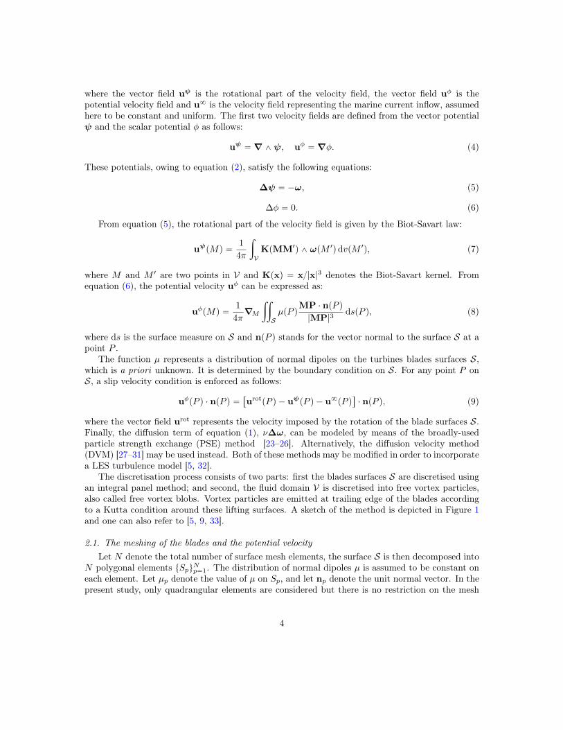
The discretisation process consists of two parts: first the blades surfaces S are discretised usingan integral panel method; and second, the fluid domain V is discretised into free vortex particles,also called free vortex blobs. Vortex particles are emitted at trailing edge of the blades accordingto a Kutta condition around these lifting surfaces. A sketch of the method is depicted in Figure 1and one can also refer to [5, 9, 33].

2.1. The meshing of the blades and the potential velocityLet N denote the total number of surface mesh elements, the surface S is then decomposed into

N polygonal elements tSpuNp“1. The distribution of normal dipoles µ is assumed to be constant oneach element. Let µp denote the value of µ on Sp, and let np denote the unit normal vector. In thepresent study, only quadrangular elements are considered but there is no restriction on the mesh

4

Blade - thin profile

Panel method Vortex method

Trailing edge - particle emission

Free vortex particles

Figure 1: Schematic cross-sectional view of a blade profile showing the respective locations of the panel method andof the particle method, respectively.

dh

Lc pNcq

LTE pNTEq

L

R

dh

ez

ey

ex

Figure 2: Description of the meshing parameters on a single turbine model reproduced from [5]. The differentmeshing characteristics are given in Table 1 of section 3.

element type and one may choose triangles, pentagons, etc., provided that the following equationsare modified accordingly. A typical turbine mesh, reproduced from [5], is illustrated on Fig. 2.

From these assumptions, it follows that equation (8) can be recast, for M P V, as

UφpMq “Nÿ

p“1

µp4π

∇M

ij

Sp

MP ¨ npP q

|MP|3dspP q. (10)

It then follows from Stokes’ formula [34–37] that

UφpMq “1

4π

Nÿ

p“1

µp

3ÿ

k“0

ż

`kp

MP

|MP|3^ dP, (11)

where `0p, `1p, `2p, `3p are the four edges of the element Sp, whose corresponding vectors may be orientedaccording to the direction of the normal np.

5

2.2. The vortex particles and the rotational velocityThe vortical fluid domain (see right hand side of Figure 1) is discretised using particles (or blobs).

The fluid properties, and particularly its vorticity field ω, are represented by a finite family of vortexparticles tPiuNP

i“1. The use of particles amounts to a Lagrangian aspect of the flow computation,where the particles are seen as material parts of the fluid that evolve according to the fluid motions.In addition, the number of particles, denoted by NP, may vary with time.

For each particle Pi, the following quantities are defined:

• Vi “ş

Pidv is the volume of particle Pi;

• Xi “ş

Pix dvVi is its position; and

• Ωi “ş

Piω dv is its vortical weight.

Each particle Pi also has its own velocity Ui “ U pXiq, which is decomposed as in equation (3)into the potential component Uφ

i “ Uφ pXiq (eq. (11)), the far-field velocity U8, and the rotationalpart Uψ

i “ UψpXiq, as mentioned previously. This last component of the velocity field can bediscretised from equation (7) by:

UψpMq “NPÿ

j“1

KεpMXjq ^Ωj , (12)

where the kernel Kε is a smoothed version of the Biot-Savart kernel K in equation (7), assumed toconverge to K when the smoothing parameter ε tends to 0 [38, 39]. The Helmholtz decompositionof equation (3) can now be expressed in a discretised form as follow:

Ui “ Uψi `Uφ

i `U8. (13)

Because the fluid is incompressible, the volume Vi of each particle is constant. On the contrary,the position, the vortical weight, as well as the velocity of the particles depend on the time t. Forclarity, the dependence of these quantity on t is omitted hereafter. Owing to the Lagrangian frame,the positions of the particles evolve according to the velocity as follows:

dXi

dt“ Ui. (14)

The equation satisfied by the vortical weight Ωi can be derived from the vorticity transport equa-tion (1):

dΩi

dt“ pΩi ¨∇qUi ` Vi pν∆ωqx“Xi

. (15)

This requires the evaluation of derivatives of the discretised velocity and vorticity fields. Thediscretised tensor field ∇Uφ can be evaluated by differentiating eq. (11), while the gradient of Uψ

can be obtained by differentiating the kernel Kε. The diffusion term pν∆ωqx“Xiis discretised using

the Particle Strength Exchange method [23–26]. Finally, a second order Runge-Kutta scheme isused for the time integration of the system of ordinary differential equations governing the evolutionof the position (eq. (14)) and vortical weight (eq. (15)).

6

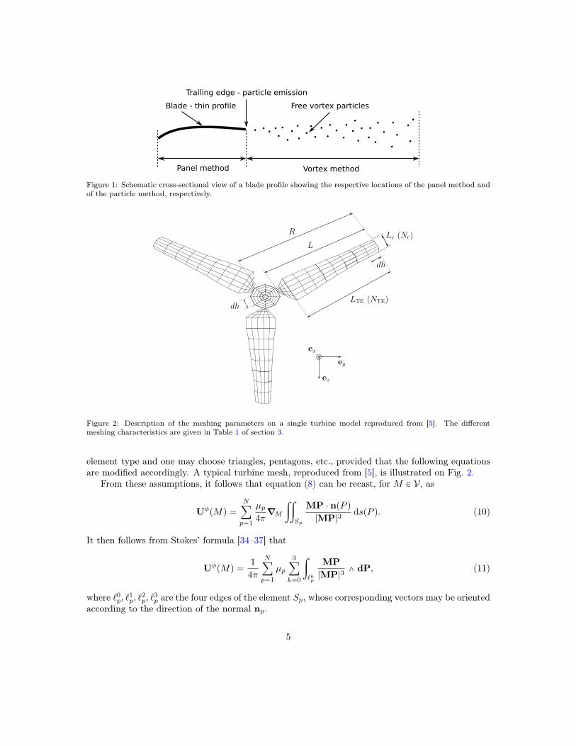
2.3. The influence matrixThe boundary condition (9) leads to a system of linear equations. Because the normal dipole

distribution on S is assumed to be uniform on each panel (piecewise constant), it can be representedby a vector of N scalar values µ “ pµjqNj“1. Then the boundary condition takes the form of a systemof N linear equations, Aµ “ b, whose solution µ enforces the boundary condition at the centres ofthe panels. The right hand side vector b “ pbiq

Ni“1 is given by:

bi ““

UrotpQiq ´UψpQiq ´U8‰

¨ ni, (16)

where Qi denotes the centre of panel Si (see Figure 3) and the velocity UψpQiq is evaluated throughequation (12). From equation (11), it follows that the so-called influence matrix, A “ paijqNi,j“1, isgiven by:

aij “ni4π¨

3ÿ

k“0

ż

`kj

QiP

|QiP|3^ dP. (17)

Qj

Qi

P 0j P 1

j

P 2jP 3

j

r1ijr0ij

Figure 3: Representation of the rkij (with k “ 0) for the evaluation of of the curvilinear integral in equation (17).The edges of panel Sj are defined as `kj “ rP

kj , P

k`1j s, where k ` 1 is taken modulo 4.

It is possible to explicitly compute the value of the integralsş

`kjQiP|QiP|

3 ^ dP. Indeed, if

we define rkij “ QiPkj , as depicted on Figure 3, then we have [34, 40, 41]:

aij “ni4π¨

3ÿ

k“0

`

|rkij | ` |rk`1ij |

˘

˜

1´rkij ¨ r

k`1ij

|rkij | |rk`1ij |

¸

rkij ^ rk`1ij

|rkij ^ rk`1ij |2

, (18)

where k ` 1 is taken modulo 4. The discrete potential velocity given by equation (11) is evaluatedusing the same geometric representation of the curvilinear integral, Qi being replaced by any pointM in V.

The coefficient aij of the matrix A represents the influence of element Sj onto element Si,which is generally different from the influence aji of element Si onto element Sj , owing to themeshing process (section 3.1). As a consequence, A is generally non-symmetric. When a singleturbine is considered, the matrix A basically represents the influence of a single turbine on itself.Figure 4 gives a schematic view of such a problem involving one single turbine. As illustrated,because the turbine is assumed to be undeformable, the rotation 9θ does not change the coefficientsof A defined in equation (18). This is generally true for any isometric transformation, as long asthe solid body is undeformable. As a matter of fact, the dot and cross products are invariant byisometric transformation, and A is thus constant with respect to time. For example, the influence of

7

(1)

(2)

(2)(2)

(1) (1)

Figure 4: Schematic view of the single turbine case.

a given panel Si on its own centre point, like the interaction referred to as (1) on Figure 4, remainsunchanged by the rotation. Likewise, the influence of a panel Sj on the centre point Qk of anotherpanel Sk pertaining to the same body (subject to the same rotation) does not change, as illustratedby interaction (2). This is the reason why direct inversion was preferred in previous works where asingle turbine was considered [5].

(1) (1)

(2)

(2)

(3) (3)

(4) (4)(5)

(5)

(1)

(2)

(3)

(4)

(5)

Figure 5: Schematic view of the twin-turbines case (n “ 2).

On the contrary, when n ą 1 turbines are concerned, the global matrix A is no longer constantover time. Each individual turbine Ti (for i “ 1, . . . , n) is discretised by a contiguous subfamily of

8

the family of panels tSpiqp uNip“1 Ă tSpu

Np“1. The matrix A then has a natural block structure:

A “

»

—

—

—

–

rA11s rA12s ¨ ¨ ¨ rA1ns

rA21s rA22s ¨ ¨ ¨ rA2ns

......

. . ....

rAn1s rAn2s ¨ ¨ ¨ rAnns

fi

ffi

ffi

ffi

fl

. (19)

To each pair of turbines pTi, Tjq corresponds a block rAijs of the influence matrix containing theinfluence of the turbine Ti on the turbine Tj . In particular, each diagonal block rAiis is a squareblock and corresponds to the well-posed problem of the influence of a single turbine on itself. Asa consequence, diagonal blocks rAiis do not change with time, owing to the arguments mentionedabove. Figure 5 depicts the simplest case of n “ 2 turbines. As an illustration, the schematicintra-turbine interactions (1) and (3), as well as (2) and (4) depicted on Fig. 5 remain unmodifiedwith the rotation of the turbines and therefore rA11s and rA22s are constant blocks. Conversely, onecan see that inter-turbines interactions are modified at each time step, for instance the schematicinteraction number (5) on Figure 5. Consequently, any extra-diagonal block rAijs, that is withi ‰ j, corresponds to the interactions between distinct turbines. Even if the rotation speeds 9θ1 and9θ2 were the same, the elements in the extra-diagonal blocks would change with time1.

2.4. Turbine definition, meshes and multi-turbines layoutIn the present study, the numerical configuration described in ref. [5] is considered, with the

“IFREMER-LOMC” blades. The reader may refer to [5, 42] for a detailed description of the turbinewe are modelling in the present paper. Because the computations are run dimensionless, theturbine radius is basically R “ 1 and the characteristic mesh size for the trailing edge is definedby dh (see Fig. 2 for details). The overlapping parameter κ “ εdh, defined as the ratio betweenthe smoothing parameter ε (see eq. (12)) and the characteristic mesh size dh (see Fig. 2), is keptapproximately constant. The mesh parameters use subsequently in this paper are described inTable 1. NTE (resp. Nhub

TE ) represents the discretisation of a blade’s trailing edge (resp. of thehub’s trailing edge). Nc (resp. Nhub

c ) represents the discretisation along the chord of the blade(resp. along the hub’s length). N represents the total number of mesh elements and is greater thanNc ˆNTE `N

hubc ˆNhub

TE owing to the discretisation of the hub’s front cross-sectional area. Eachmesh is referenced using a label of the form NcˆNTE. The last five meshes, however, correspond toa slightly different geometry, with a longer hub, while the blade geometry and meshing remain thesame. The meshes corresponding to those geometries will thus be labeled Nc ˆNTE

˚ to distinguishthem from their short hub counterpart. For instance, the very first mesh in Table 1 is labeled5 ˆ 5, while the very last one is labeled 5 ˆ 23˚. Considering a single turbine configuration, withthe meshes presented in Table 1, the size of the influence matrix A ranges approximately from200ˆ 200 to 2,000ˆ 2,000. For a 10-turbines configuration with the finer turbine discretisation, a20,000ˆ20,000 (non sparse) matrix can eventually be considered. And in a close future, even moreturbines with finer discretisations are expected.

Figure 6 depicts a generic turbine layout. In that matter, a generic notation needs to be definedin order to synthetically describe the layout. Let us denominate by Anxˆny

xD,yD a configuration with

1One particular scenario is when the rotation speeds are the same and the turbines are perfectly aligned withthe rotation axis, in which case they can be considered as a single body subject to the same rotation, and then thematrix remains constant.

9

ε Nc NTE Nhubc Nhub

TE N β γ

0.200 5 5 6 6 182 0.0629 00.150 5 7 6 8 233 0.0903 00.100 5 11 6 12 339 0.1335 00.075 5 15 6 16 446 0.1594 10.050 5 23 6 24 666 0.1765 1

0.200 10 5 12 6 338 0.0284 00.150 10 7 12 8 431 0.0397 00.100 10 11 12 12 621 0.0626 00.075 10 15 12 16 812 0.1110 00.050 10 23 12 24 1200 0.1765 1

0.200 15 5 18 6 494 0.0281 00.150 15 7 18 8 629 0.0300 00.100 15 11 18 12 903 0.0398 00.075 15 15 18 16 1178 0.0704 10.050 15 23 18 24 1734 0.1544 1

0.200 5 5 58 6 488 0.0624 00.150 5 7 58 8 641 0.1000 20.100 5 11 58 12 964 0.1451 10.075 5 15 58 16 1278 0.1594 10.050 5 23 58 24 1914 0.1766 2

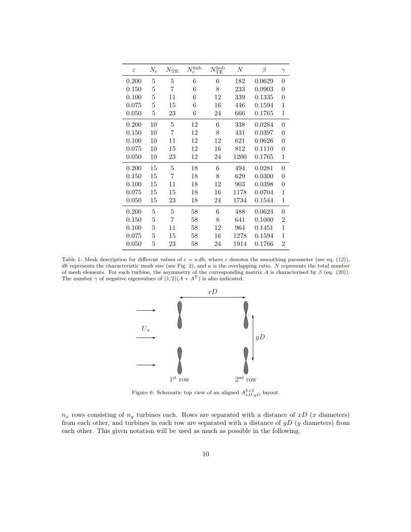
Table 1: Mesh description for different values of ε “ κ dh, where ε denotes the smoothing parameter (see eq. (12)),dh represents the characteristic mesh size (see Fig. 2), and κ is the overlapping ratio. N represents the total numberof mesh elements. For each turbine, the asymmetry of the corresponding matrix A is characterised by β (eq. (20)).The number γ of negative eigenvalues of p12qpA`AT q is also indicated.

U8

xD

yD

1st row 2nd row

Figure 6: Schematic top view of an aligned A2ˆ2xD,yD layout.

nx rows consisting of ny turbines each. Rows are separated with a distance of xD (x diameters)from each other, and turbines in each row are separated with a distance of yD (y diameters) fromeach other. This given notation will be used as much as possible in the following.

10

3. Iterative solver approach

Owing to the unsteady frame of the computations, the influence system Aµ “ b described insection 2.3 is solved at each time step. When a single turbine is considered, the influence matrixA is inverted and stored prior to the iterations, as mentioned earlier. And a single matrix-vectormultiplication is then required at each time step. In the case of multiple turbine interactions [6], A isno longer constant with respect to time (see Figure 5). Moreover, because there are several turbines,the size of the matrix A increases and matrix inversion at each time step becomes prohibitive interms of CPU time consumption. For other numerical methods where the linear system is thecore of the method, a very efficient solver needs to be used, using for example dedicated libraries.However, in the framework of particle methods with boundary integral methods (using Kutta-Joukowski emission, etc.), simple linear system resolutions are commonly used, although it canbecome very costly is some cases. In the following, an attempt to propose a fast and rigorousmethod is presented for unsteady problems with multi-bodies in the Lagrangian vortex particlesframework.

3.1. Matrix characterisationWhen attempting to choose the best numerical implementation, several questions arise such

as: is the influence matrix sparse? symmetric? diagonally dominant? positive-definite? From thedefinition of aij (equations (17) and (18)) one can see that aij ‰ 0 for all pi, jq, except in some veryhypothetical geometrical turbine design. As a consequence, the matrix A is generally not sparse.

(a) Single turbine, mesh 15 ˆ 23. (b) A2ˆ24D,1D, meshes 15 ˆ 15.

Figure 7: Representation of |aij | for (left) a single turbine 15ˆ 23, corresponding to a matrix of size N “ 1,734; and(right) n “ 4 identical turbines with meshes 15ˆ15 and layout A2ˆ2

4D,1D, corresponding to a matrix of size N “ 4,712.The meshes are detailed in Table 1.

Despite the formal symmetry of the original continuous problem, the matrix A is not symmetriceither. As a matter of proof, aij depends on two geometrical items that are, the mesh elementsurface Sj (see eq. (17) in a continuous form, and eq. (18) in a discrete form) and the mesh elementnormal ni (see eq. (18)). Depending on the mesh element shape (during the mesh generation) andthe regularity of these surface elements (if the quadrangle meshes are similar to squares of size

11

dh2), A might not be far from symmetry, as can be observed on Figure 7. In order to quantify thisasymmetry, let β represent the ratio of the norm of the anti-symmetric part of A (i.e. 12pA´AT q)to the norm of A:

β “

›

›p12q`

A´AT˘›

›

A. (20)

One can see on Table 1 that β is rather small. This tends to corroborate that A is nearly symmetric.But when choosing the numerical implementation, the use of proper symmetric matrices cannot beargued.

Regarding the diagonal-dominance of A, owing to the gravitational-like interaction of equa-tion (17), a diagonal dominance could have been expected. Nevertheless this mainly depends onthe mesh element ordering during the mesh generation together with the relative distance betweenthese elements. Even with a special care during the meshing phase, a real diagonal dominancecannot be achieved. As a matter of proof, two plots of |aii| ´

ř

j‰i |aij | for different meshes andturbines configurations are depicted on Figure 8. On Figure 8a, the spiky parts correspond to theauto-influence of the blades on themselves, while the rest (on the right hand side) mainly corre-sponds to the influence with the hub surface. However, from Figure 8a, one can clearly observe thatthe matrix is not diagonally dominant. This property of non-diagonal dominance is not improvedby adding more turbines in the configuration, as it actually tends to increase the weight of extra-diagonal terms. This statement is further corroborated by the results of Fig. 8b for a two-turbinesconfiguration. Similar results (not presented here) were also obtained for larger numbers of turbinesand different meshes.

−40

−20

0

20

40

60

80

100

120

1 1178200 400 600 800 1000

|aii|−

∑ j6=i|a

ij|

i

(a) Single turbine, mesh 15 ˆ 15.

−40

−20

0

20

40

60

80

100

120

1 3468500 1000 1500 2000 2500 3000

|aii|−

∑ j6=i|a

ij|

i

(b) A2ˆ12D , meshes 15 ˆ 23.

Figure 8: Plot of |aii| ´ř

j‰i |aij | with colouring of the sign for (left) a single turbine 15 ˆ 15, corresponding toa matrix of size N “ 1,178; and (right) n “ 2 turbines with meshes 15 ˆ 23, corresponding to a matrix of sizeN “ 3,468. Blue means positive and red means negative. See Table 1 for mesh characteristics.

The relative weakness of the influence terms between distinct turbines is visible by the factthat Figure 8b looks like (but is indeed different from) periodic repetitions of a single pattern.Adding more turbines to the layout even emphasises this impression. Very short distances betweenturbines were chosen here in order to emphasise the influence of these extra-diagonal terms. Shorterdistances between turbines could further increase the influence between turbines but may lead tonon-physical turbine configurations. Indeed, for marine current turbine array configurations, theminimum lateral spacing is always of the order of one diameter (see [4, 16, 43]). The longitudinalspacing is generally of the order of magnitude of several diameters (between 4D to 6D for [4],minimum 10 diameters for [44], etc.) However, a qualitative observation of Figure 7b tends to

12

indicate that the matrices have a block-diagonal dominance. This observation will have a significantimportance in the following of the paper (section 3.3).

Finally, let us determine whether the matrix A is positive definite. A general non-symmetricmatrix A is positive definite if its symmetric part (i.e. p12qpA`AT q) is symmetric positive definite(SPD). In addition, a symmetric matrix is SPD if all its eigenvalues are positive. The number γof negative eigenvalues of p12qpA ` AT q is reported in Table 1 for single turbine configurations.It shows that the influence matrices are not always positive definite. In particular, the matricesp12qpA ` AT q corresponding to the finer discretisations (Nc ˆ 23 and 5 ˆ 23˚) have at least onenegative eigenvalue (and at most two for 5 ˆ 23˚). When several turbines configurations are con-sidered, the number γ of negative eigenvalues, reported in Table 2, seems to be the sum of thenumber of negative eigenvalues of the separate single turbine case. One possible explanation couldbe the dominance of the diagonal blocks as compared to the other blocks of the matrix. Indeedit would follow that the matrix p12qpA ` AT q has essentially the same spectrum as the matrixp12qpK `KT q, where K is the block diagonal matrix whose blocks are the diagonal blocks of A,introduced later in section 3.3 (see eq. (22)).

Meshes γ

p5ˆ 23, 5ˆ 23q 2p10ˆ 5, 10ˆ 5q 0p15ˆ 23, 15ˆ 23q 2p5ˆ 23, 5ˆ 15q 2

Table 2: Number γ of negative eigenvalues of the matrix p12qpA`AT q for a configuration of n “ 2 turbines modelledwith different meshes for layout A2ˆ1

2D . The first three cases use the same mesh for both turbines, while the fourthcase uses two different meshes.

3.2. Chosen implementationFrom the previous section, it appears that iterative methods (in particular Krylov methods)

would be the best suited to solve the influence system described in section 2.3. A classical LUdecomposition would require OpN3q operations, which is unaffordable in terms of CPU time forlarge matrices. An iterative method is used as a way to reduce computational cost. Typically,an iterative method only involves a few matrix-vector multiplications per iteration, thus requiringOpmN2q operations for a total of m iterations. An iterative method is thus more interesting thana direct solver provided that it converges (to a desired level of accuracy) in less than N iterations.This is generally the case of Krylov methods.

The chosen method is the Bi-Conjugate Gradient Stabilised (abbreviated Bi-CGSTAB) de-scribed in [22]. The Bi-CGSTAB algorithm is a Krylov method adapted to general linear systems.This algorithm can be seen as an improvement of other general methods such as the ConjugateGradients-Squared method [22]. Because the Conjugate Gradient (CG) is designed for symmetricmatrices, this method might not be the best choice here. However, as the considered matrices areonly slightly non-symmetric, a CG implementation is also tested in the sequel. Finally, a classicalJacobi implementation is also considered for general comparison. The Jacobi method is a classicaliterative method for solving linear systems. It is simple to implement and to parallelize. However,its convergence is not guaranteed for matrices that are not diagonally dominant, and may be veryslow.

13

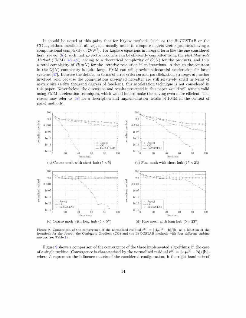
It should be noted at this point that for Krylov methods (such as the Bi-CGSTAB or theCG algorithms mentioned above), one usually needs to compute matrix-vector products having acomputational complexity of OpN2q. For Laplace equations in integral form like the one consideredhere (see eq. (8)), such matrix-vector products can be efficiently computed using the Fast MultipoleMethod (FMM) [45–48], leading to a theoretical complexity of OpNq for the products, and thusa total complexity of OpmNq for the iterative resolution in m iterations. Although the constantin the OpNq complexity is quite large, FMM can still provide substantial acceleration for largesystems [47]. Because the details, in terms of error criterion and parallelization strategy, are ratherinvolved, and because the computations presented hereafter are still relatively small in terms ofmatrix size (a few thousand degrees of freedom), this acceleration technique is not considered inthis paper. Nevertheless, the discussion and results presented in this paper would still remain validusing FMM acceleration techniques, which would indeed make the solving even more efficient. Thereader may refer to [48] for a description and implementation details of FMM in the context ofpanel methods.

1e-16

1e-13

1e-10

1e-07

0.0001

0.1

100

0 20 40 60 80 100

norm

alise

dre

sidua

l

iterations

JacobiCGBi-CGSTAB

(a) Coarse mesh with short hub (5 ˆ 5)

1e-16

1e-13

1e-10

1e-07

0.0001

0.1

100

0 20 40 60 80 100

norm

alise

dre

sidua

l

iterations

JacobiCGBi-CGSTAB

(b) Fine mesh with short hub (15 ˆ 23)

1e-16

1e-13

1e-10

1e-07

0.0001

0.1

100

0 20 40 60 80 100

norm

alise

dre

sidua

l

iterations

JacobiCGBi-CGSTAB

(c) Coarse mesh with long hub (5 ˆ 5˚)

1e-16

1e-13

1e-10

1e-07

0.0001

0.1

100

0 20 40 60 80 100

norm

alise

dre

sidua

l

iterations

JacobiCGBi-CGSTAB

(d) Fine mesh with long hub (5 ˆ 23˚)

Figure 9: Comparison of the convergence of the normalised residual rpiq “ Aµpiq ´ bb as a function of theiterations for the Jacobi, the Conjugate Gradient (CG) and the Bi-CGSTAB methods with four different turbinemeshes (see Table 1).

Figure 9 shows a comparison of the convergence of the three implemented algorithms, in the caseof a single turbine. Convergence is characterised by the normalised residual rpiq “ Aµpiq ´ bb,where A represents the influence matrix of the considered configuration, b the right hand side of

14

the influence system, and µpiq the approximation of the solution µ given by the ith iteration of thealgorithm. The Jacobi method seems to converge quite slowly and after 100 iterations, a normalisedresidual of 10´3 is hardly achieved. The CG method converges a little faster. The Bi-CGSTAB isthe only method to reach machine precision in less than 100 iterations in the single turbine case.

1e-16

1e-13

1e-10

1e-07

0.0001

0.1

100

0 20 40 60 80 100

norm

alise

dre

sidua

l

iterations

JacobiCGBi-CGSTAB

(a) A2ˆ22D,1D with meshes 5 ˆ 5.

1e-16

1e-13

1e-10

1e-07

0.0001

0.1

100

0 20 40 60 80 100

norm

alise

dre

sidua

l

iterations

JacobiCGBi-CGSTAB

(b) A2ˆ22D,1D with meshes 15 ˆ 23.

1e-16

1e-13

1e-10

1e-07

0.0001

0.1

100

0 20 40 60 80 100

norm

alise

dre

sidua

l

iterations

JacobiCGBi-CGSTAB

(c) A2ˆ24D,1D with meshes 5 ˆ 5˚.

1e-16

1e-13

1e-10

1e-07

0.0001

0.1

100

0 20 40 60 80 100

norm

alise

dre

sidua

l

iterations

JacobiCGBi-CGSTAB

(d) A2ˆ24D,1D with meshes 5 ˆ 23˚.

Figure 10: Comparison of the convergence of the normalised residual for the Jacobi, the Conjugate Gradient (CG)and the Bi-CGSTAB methods for two different layouts of 4 turbines (see Table 1).

Figure 10 shows convergence plots for 4-turbine configurations. Similarly to the single turbinecase, the Bi-CGSTAB behaves better than the CG and Jacobi methods. For instance, in theconfiguration depicted on Figure 10a, the Bi-CGSTAB reaches the same precision (rpiq « 10´4) inless than 20 iterations as the CG does in 80 iterations. Furthermore, the CG does not converge forthe last two configurations (Fig. 10c–10d). As mentioned previously, this is most likely due to thefact that the CG is not suited to non-symmetric matrices. Its use is thus unsafe as the directions arenot properly conjugate (specifically, the metric used for conjugation is not a proper inner product),which means that the resulting Krylov subspace is erroneous. For nearly symmetric matrices, theerroneous directions might still be good enough to keep the solution improving iteratively. On theother hand, some matrices may drive the solution outside the theoretical Krylov space, potentiallyleading to situations from which the CG iterations cannot recover. At any rate, even considering thefact that the Bi-CGSTAB requires twice as much computation (in terms of matrix-vector products)as the CG, the Bi-CGSTAB still appears to be the most efficient method in solving this problem.

15

3.3. PreconditioningIt is well-known that an adequate preconditioner may dramatically improve the convergence of

such iterative methods. The purpose of preconditioning is basically to improve the condition numberof the matrix of the linear system. In the sequel, we will focus on left preconditioning, which consists,for a linear system of the form Ax “ b, in solving the equivalent system M´1Ax “ M´1b whereM´1A, the preconditioned matrix, has a smaller condition number than A. The matrix M (orsometimes M´1 itself) is then called the preconditioner. One first simple choice of preconditionerwould be the Jacobi preconditioner, which consists in taking the diagonal of A as the preconditionerM . Let us denote it by D. It has the following definition:

D “ pdijq “ diagpAq, dij “ aiiδij , @i, j “ 1, . . . , N, (21)

where δij denotes the Kronecker delta. The advantage of such a preconditioner is that its inverseis easy to compute. As a matter of fact, D´1 is simply the diagonal matrix whose elements are theinverses of those of D.

Taking advantage of the structure and evolution of the matrix (with respect to the time-stepsof the unsteady simulation), let us now define a more appropriate preconditioner. First, recallthat the matrix of the influence equation has a natural block structure (see eq. (19)) and thatits diagonal blocks have essentially larger coefficients than the others (see Fig. 7). Moreover, thediagonal blocks of the matrix are constant over time. This fact allows the diagonal blocks to be usedfor preconditioning. Let K be the block diagonal matrix whose blocks correspond to the diagonalblocks of the matrix A. The matrix K is then used as the preconditioning matrix. Its advantage isthat its inverse is also a block diagonal matrix consisting of the inverses of the blocks of A. Moreprecisely, K and its inverse K´1 have the following form:

K “

»

—

—

—

—

–

rA11s 0 ¨ ¨ ¨ 0

0 rA22s...

.... . . 0

0 ¨ ¨ ¨ 0 rAnns

fi

ffi

ffi

ffi

ffi

fl

, K´1 “

»

—

—

—

—

–

rA11s´1

0 ¨ ¨ ¨ 0

0 rA22s´1 ...

.... . . 0

0 ¨ ¨ ¨ 0 rAnns´1

fi

ffi

ffi

ffi

ffi

fl

. (22)

Since the matrix K is constant over time, its inversion can be performed at the beginning ofthe simulation. This can be done by using a direct method. Indeed, the diagonal blocks of thematrix A are invertible since they correspond to the well defined problem of the influence of a singleturbine on itself. In what follows, the matrix K will be called the block Jacobi (abbreviated BJac.)preconditioner.

Tables 3 and 4 show examples of the number of iterations for unpreconditioned and precondi-tioned (with the Jacobi (Jac.) and the block Jacobi (BJac.) preconditioners) for both the CG andthe Bi-CGSTAB. Let us first make a few comments on the simple Jacobi preconditioner mentionedpreviously. When combined with the CG method, the Jacobi preconditioner actually makes theiterations worse (degrading as compared to the unpreconditioned version). This combination of theJacobi preconditioner with the CG is thus inefficient here. However, the Jacobi preconditioner com-bined with the Bi-CGSTAB always improves the convergence (see Tables 3 and 4). As a matter offact, even in the worse cases of Table 4, approximately half as many iterations are required to reachmachine precision with the use of the Jacobi preconditioner (as compared to the unpreconditionedversion).

16

No preconditioning Jac. precond. BJac. precond.

Mesh Jacobi CG Bi-CGSTAB CG Bi-CGSTAB CG Bi-CGSTAB

5ˆ 5 (10´12) (10´10) 47 (10´3) 33 5 35ˆ 7 (10´12) 329 53 (10´5) 34 5 35ˆ 11 (10´11) (10´12) 52 (10´7) 33 5 35ˆ 15 (10´10) (10´4) 67 (10´1) 39 5 35ˆ 23 (10´8) (10´5) 89 (101) 37 5 3

10ˆ 5 (10´9) (10´6) 76 (10´2) 41 5 310ˆ 7 (10´9) (10´11) 89 (10´8) 42 5 310ˆ 11 (10´9) 219 88 (10´8) 42 5 310ˆ 15 (10´8) 373 83 (10´3) 43 5 310ˆ 23 (10´7) (10´12) 92 (100) 43 5 3

15ˆ 5 (10´8) (10´6) 96 (10´3) 49 5 315ˆ 7 (10´8) (10´12) 101 (10´4) 52 5 315ˆ 11 (10´8) 218 101 (10´10) 49 5 315ˆ 15 (10´8) 224 109 (10´7) 47 5 315ˆ 23 (10´7) 471 103 (10´4) 50 5 3

Table 3: Number of iterations before convergence for the different algorithms using layout A2ˆ22D,1D and different mesh

sizes (with short hubs). The values in the entries represents the first number of iterations i for which the relativeresidual rpiq “ Aµpiq ´ bb reaches machine precision ε « 2.2 ¨ 10´16. When the algorithm did not reach therequired precision before 500 iterations, the order of magnitude of the final normalised residual is given betweenparentheses.

No preconditioning Jac. precond. BJac. precond.

Mesh Jacobi CG Bi-CGSTAB CG Bi-CGSTAB CG Bi-CGSTAB

5ˆ 5˚ (10´2) (10´2) 194 (100) 94 5 35ˆ 7˚ (10´2) (10´2) 193 (10´2) 123 5 35ˆ 11˚ (10´1) (101) 269 (101) 150 5 35ˆ 15˚ (10´1) (101) 301 (100) 164 5 35ˆ 23˚ (10´1) (100) 288 (109) 143 5 3

Table 4: Number of iterations before convergence for the considered algorithms using layout A2ˆ24D,1D and different

mesh sizes (with long hubs). See also Table 3.

Second, using the block Jacobi preconditioner, the improvement appears clearly as the numberof iterations decreases dramatically for the CG and Bi-CGSTAB algorithms. For all of the casesconsidered, the number of iterations necessary to obtain a relative residual rpiq using the precondi-tioned Bi-CGSTAB below the machine precision is 3. The CG method does not reach the requiredprecision within a reasonable number of iterations for several unpreconditioned computations. Atthe same time, it converges in 5 iterations when preconditioned in a block Jacobi manner. Fur-thermore, with this preconditionning, the number of iterations does not change when the meshstructure is modified.

17

To further illustrate the effectiveness of this BJac. preconditioner, Figure 11 shows the con-vergence of the BJac. preconditioned methods (CG and Bi-CGSTAB) compared to the basic un-preconditioned Jacobi iterative method. After 200 iterations, the latter still has a residual greaterthan 10´6, while the preconditioned CG and BI-CGSTAB get below 10´6 after 2 and 1 iteration(s)respectively. It should be mentioned that the CG is slightly faster than the Bi-CGSTAB due to thefact that the latter requires twice as many matrix-vector multiplications at each iteration. Howeverit has to be recalled that the use of the CG is still not safe here due to the general asymmetry ofthe matrix A (see section 3.2).

1e-20

1e-17

1e-14

1e-11

1e-08

1e-05

0.01

0 50 100 150 200

norm

alise

dre

sidua

l

iterations

Unprecond. JacobiPrecond. CGPrecond. Bi-CGSTAB

(a) 200 iterations

1e-20

1e-17

1e-14

1e-11

1e-08

1e-05

0.01

0 1 2 3 4 5 6 7 8no

rmal

ised

resid

ual

iterations

Unprecond. JacobiPrecond. CGPrecond. Bi-CGSTAB

(b) First eight iterations

Figure 11: Comparison of the convergence of the normalised residual rpiq for the unpreconditioned Jacobi method,the BJac. preconditioned CG and the BJac. preconditioned Bi-CGSTAB. The configuration corresponds to analigned A2ˆ2

2D,1D layout with meshes 15ˆ 23.

To conclude, an example of the effect of the preconditioners on the matrix A is shown onFigure 12. In particular, one can see that the Jacobi preconditioner leaves the matrix with manylarge values outside the diagonal.

(a) Matrix A.Unprecond.

(b) Matrix D´1A.Jac. precond.

(c) Matrix K´1A.BJac. precond.

Figure 12: Comparison of the structures of the non preconditioned and preconditioned influence matrix for the 4meshes 5ˆ 5˚ in configuration A2ˆ2

4D,1D of Table 4.

18

4. Application: computations of several turbines in interaction

The following paragraphs present some results as an illustrative application of the iterative solverapproach described above. Here, two configurations of elementary interactions between marine cur-rent turbines in close proximity are presented. Marine current turbines are considered here becauseit corresponds to the background research topics of our research team. However, applications towind turbines could be considered without any restriction. The results presented here correspondto computations that were recently made accessible thanks to CPU time improvements brought bythe iterative solver approach. A complete numerical study is to be performed in the near future,including the influence of the distance between turbines, as well as other numerical and physicalparameters. Although qualitative results of wake interaction in a three-turbine setting are brieflypresented, the main focus of this section will remain on the quantitative assessment of the savingsachieved in terms of computational time thanks to the iterative solver approach presented in theprevious sections.

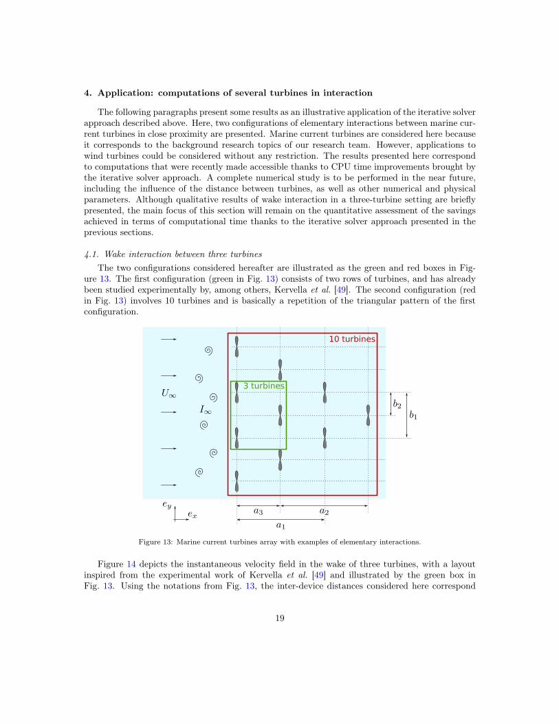
4.1. Wake interaction between three turbinesThe two configurations considered hereafter are illustrated as the green and red boxes in Fig-

ure 13. The first configuration (green in Fig. 13) consists of two rows of turbines, and has alreadybeen studied experimentally by, among others, Kervella et al. [49]. The second configuration (redin Fig. 13) involves 10 turbines and is basically a repetition of the triangular pattern of the firstconfiguration.

3 turbines

10 turbines

Figure 13: Marine current turbines array with examples of elementary interactions.

Figure 14 depicts the instantaneous velocity field in the wake of three turbines, with a layoutinspired from the experimental work of Kervella et al. [49] and illustrated by the green box inFig. 13. Using the notations from Fig. 13, the inter-device distances considered here correspond

19

to a3 “ 4D and b1 “ 2b2 “ 2D. The instantaneous velocity field was obtained at t « 28.2 s(physical time) in the unsteady computation, corresponding to 399 unsteady iterations of time stepdt “ 0.07066 s, using three meshes 5ˆ 5˚ from Table 1. The reader may refer to [5] for a discussionon how the time step is chosen. This computation corresponds to the coarsest mesh discretisation,and improvements in the quality of the results are expected in the near future. However, theseresults are still interesting qualitatively as many physical aspects are already observable even forthese discretisations, such as the wake interaction that is clearly visible in Fig. 14 where the wakeof the first row of turbines reaches the third turbine. As already discussed, a complete surveyincluding several turbine layouts, several inter-device distances and other physical parameters isscheduled in the near future. Comparison with the experimental work of Kervella et al. [49] willalso be considered.

y∗

x∗

-2

-1.5

-1

-0.5

0

0.5

1

1.5

2

-1 0 1 2 3 4 5 6 7 8 u∗

0.3

0.4

0.5

0.6

0.7

0.8

0.9

1

1.1

Figure 14: Numerical wake for the 3-turbine configuration (green in Fig. 13) at TSR “ 2. The inter-device distancesare a3 “ 4D and b1 “ 2b2 “ 1D using the notations from Fig. 13.

4.2. Assessment of CPU time savings using the present approachIn order to have an assessment of the CPU time savings obtained with the present approach,

the last five meshes of Table 1, corresponding to the longer hub with Nhubc “ 58, were tested

on the 3-turbine and 10-turbine configurations depicted in Fig. 13. The 3-turbine configurationcorresponds exactly to the one presented in Fig. 14. These meshes were chosen for two reasons:first because the longer hub corresponds to the real size of the turbine hub used in the experiments(see [5, 42]), and second because the mesh 5 ˆ 23˚ also corresponds to the larger number of meshelements. In the case of 10 turbines in interaction, this last mesh will be considered as a criticalcase with a 19,140ˆ 19,140 matrix system to be solved at each time step either by direct inversionor by iterative solve using the preconditioned Bi-CGSTAB method.

Table 5 presents the particle emission time for both configuration (with 3 and 10 turbines) anddifferent meshes. This total emission time ttot includes the time t1 spent by the matrix update(eq. (18)) and the emitted particle initialisation, the time t2 spent either by the system resolutionin the case of the use of Bi-CGSTAB or by the matrix inversion and matrix-vector multiplication forthe direct method case, and the time t3 spent by the computation of the right-hand-side (eq. (16)).These times were obtained from the first 10 iterations where an average was performed over thelast 9 values, the first iteration being discarded. An average over the first 100 iterations was alsoperformed without significant changes in the resulting values. Except for the computation of the

20

Mesh precond. Bi-CGSTAB Inversion

3 turb. t1 t2 t3 ttot t1 t2 t3 ttot

5ˆ 5˚ 3.2ˆ 10´3 3.1ˆ 10´3 3.0ˆ 10´3 9.4ˆ 10´3 4.4ˆ 10´3 4.6ˆ 10´2 3.2ˆ 10´3 5.3ˆ 10´2

5ˆ 7˚ 5.2ˆ 10´3 3.1ˆ 10´3 6.2ˆ 10´3 1.4ˆ 10´2 8.1ˆ 10´3 9.4ˆ 10´2 6.8ˆ 10´3 1.1ˆ 10´1

5ˆ 11˚ 1.3ˆ 10´2 3.7ˆ 10´3 1.6ˆ 10´2 3.2ˆ 10´2 1.9ˆ 10´2 2.8ˆ 10´1 1.6ˆ 10´2 3.1ˆ 10´1

5ˆ 15˚ 2.2ˆ 10´2 3.8ˆ 10´3 2.6ˆ 10´2 5.2ˆ 10´2 3.0ˆ 10´2 5.8ˆ 10´1 2.6ˆ 10´2 6.3ˆ 10´1

5ˆ 23˚ 4.8ˆ 10´2 4.8ˆ 10´3 6.0ˆ 10´2 1.1ˆ 10´1 6.3ˆ 10´2 3.5ˆ 10`0 6.0ˆ 10´2 3.6ˆ 10`0

10 turb. t1 t2 t3 ttot t1 t2 t3 ttot

5ˆ 5˚ 4.4ˆ 10´2 4.8ˆ 10´3 4.4ˆ 10´2 9.3ˆ 10´2 4.7ˆ 10´2 1.1ˆ 10`0 4.5ˆ 10´2 1.2ˆ 10`0

5ˆ 7˚ 7.2ˆ 10´2 7.0ˆ 10´3 7.4ˆ 10´2 1.5ˆ 10´1 7.8ˆ 10´2 3.0ˆ 10`0 7.5ˆ 10´2 3.2ˆ 10`0

5ˆ 11˚ 1.5ˆ 10´1 3.5ˆ 10´2 1.6ˆ 10´1 3.5ˆ 10´1 1.7ˆ 10´1 1.7ˆ 10`1 1.6ˆ 10´1 1.7ˆ 10`1

5ˆ 15˚ 2.6ˆ 10´1 5.1ˆ 10´2 2.8ˆ 10´1 5.9ˆ 10´1 3.4ˆ 10´1 4.4ˆ 10`1 2.8ˆ 10´1 4.4ˆ 10`1

5ˆ 23˚ 5.5ˆ 10´1 9.0ˆ 10´2 6.3ˆ 10´1 1.3ˆ 10`0 6.1ˆ 10´1 1.5ˆ 10`2 6.3ˆ 10´1 1.5ˆ 10`2

Table 5: Total emission time ttot (in seconds) and its decomposition for each mesh of Table 5. Both the developed pre-conditioned Bi-CGSTAB and the Direct approaches are presented for the 3-turbine and the 10-turbine configurations.

right-hand-side, where the time t3 increases with the number of emitted particles, the other timesremain nearly identical regardless of the global iteration in the unsteady computation.

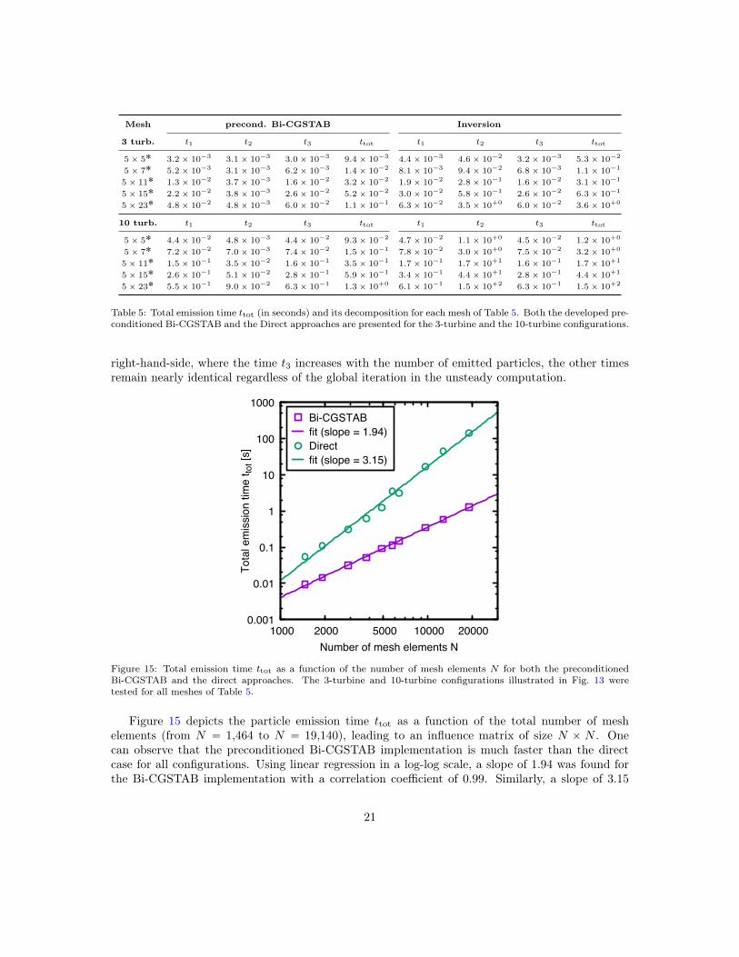
Figure 15: Total emission time ttot as a function of the number of mesh elements N for both the preconditionedBi-CGSTAB and the direct approaches. The 3-turbine and 10-turbine configurations illustrated in Fig. 13 weretested for all meshes of Table 5.

Figure 15 depicts the particle emission time ttot as a function of the total number of meshelements (from N “ 1,464 to N “ 19,140), leading to an influence matrix of size N ˆ N . Onecan observe that the preconditioned Bi-CGSTAB implementation is much faster than the directcase for all configurations. Using linear regression in a log-log scale, a slope of 1.94 was found forthe Bi-CGSTAB implementation with a correlation coefficient of 0.99. Similarly, a slope of 3.15

21

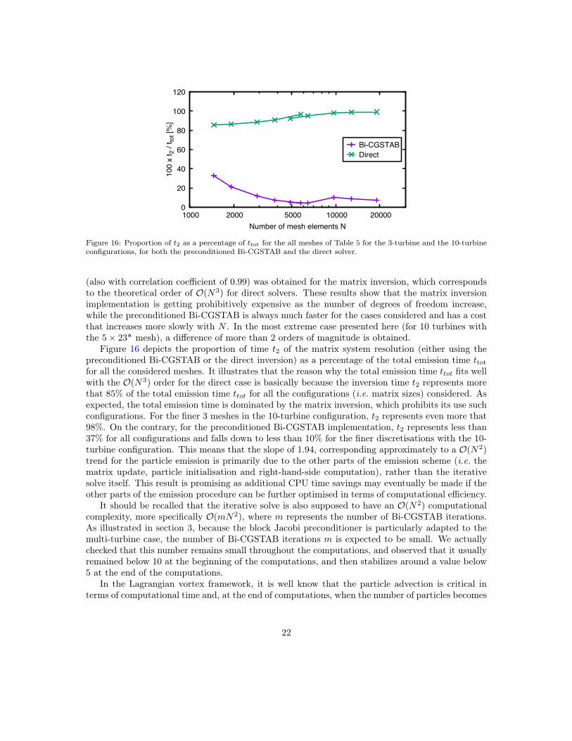
Figure 16: Proportion of t2 as a percentage of ttot for the all meshes of Table 5 for the 3-turbine and the 10-turbineconfigurations, for both the preconditioned Bi-CGSTAB and the direct solver.

(also with correlation coefficient of 0.99) was obtained for the matrix inversion, which correspondsto the theoretical order of OpN3q for direct solvers. These results show that the matrix inversionimplementation is getting prohibitively expensive as the number of degrees of freedom increase,while the preconditioned Bi-CGSTAB is always much faster for the cases considered and has a costthat increases more slowly with N . In the most extreme case presented here (for 10 turbines withthe 5ˆ 23˚ mesh), a difference of more than 2 orders of magnitude is obtained.

Figure 16 depicts the proportion of time t2 of the matrix system resolution (either using thepreconditioned Bi-CGSTAB or the direct inversion) as a percentage of the total emission time ttotfor all the considered meshes. It illustrates that the reason why the total emission time ttot fits wellwith the OpN3q order for the direct case is basically because the inversion time t2 represents morethat 85% of the total emission time ttot for all the configurations (i.e. matrix sizes) considered. Asexpected, the total emission time is dominated by the matrix inversion, which prohibits its use suchconfigurations. For the finer 3 meshes in the 10-turbine configuration, t2 represents even more that98%. On the contrary, for the preconditioned Bi-CGSTAB implementation, t2 represents less than37% for all configurations and falls down to less than 10% for the finer discretisations with the 10-turbine configuration. This means that the slope of 1.94, corresponding approximately to a OpN2q

trend for the particle emission is primarily due to the other parts of the emission scheme (i.e. thematrix update, particle initialisation and right-hand-side computation), rather than the iterativesolve itself. This result is promising as additional CPU time savings may eventually be made if theother parts of the emission procedure can be further optimised in terms of computational efficiency.

It should be recalled that the iterative solve is also supposed to have an OpN2q computationalcomplexity, more specifically OpmN2q, where m represents the number of Bi-CGSTAB iterations.As illustrated in section 3, because the block Jacobi preconditioner is particularly adapted to themulti-turbine case, the number of Bi-CGSTAB iterations m is expected to be small. We actuallychecked that this number remains small throughout the computations, and observed that it usuallyremained below 10 at the beginning of the computations, and then stabilizes around a value below5 at the end of the computations.

In the Lagrangian vortex framework, it is well know that the particle advection is critical interms of computational time and, at the end of computations, when the number of particles becomes

22

Figure 17: Emission time ttot compared with advection time for the first 130 iterations of a 10-turbine configurationusing 5ˆ 23˚ meshes.

very large as compared to the constant number of mesh elements, the emission procedure is expectedto represent only a minor fraction of total CPU time within a given unsteady iteration. This isgenerally true and this was the case for a single turbine configuration. However, this is generally nolonger the case for the 10-turbine configurations presented here. To illustrate this, Figure 17 depictsthe total emission time ttot for both the pre-conditioned Bi-CGSTAB and the direct solver comparedto the advection time for the first 130 iterations of the 10-turbine configuration using 5ˆ23˚ meshes.On this figure, it can be observed that the advection time is increasing with the number of iterations(or equivalently the physical time), which was expected because of the increasing number of emittedparticles, and hence of total particles, as the computation progresses. Additionally, one can observethat the total emission time for the direct approach never becomes lower than the advection time,even after 130 iterations where 120,832 particles are involved. At this stage, it is still the beginningof the wake interaction computation but it can be easily understood that the considered emissiontime will never become negligible and, although it may, after a large number of iterations, becomesmaller than the advection time, it will still represent a large amount of CPU time per iteration.On the contrary, with the proposed preconditioned Bi-CGSTAB implementation, the total emissiontime ttot always remains lower than the advection time, and rapidly becomes negligible with nearlyan order of magnitude after a 100 iterations. This last Figure 17 really confirms the need of such animplementation in order to undertake more accurate computations of several turbines in interaction.

5. Conclusion

The paper presents the recent numerical development carried out on unsteady 3D software [5]developed at LOMC in partnership with IFREMER. These developments were necessary in thecase of several turbines (marine or wind turbines) in order to reduce the computational cost ofsuch simulations. Indeed, a linear system needs to be solved at each time step in order to enforcethe boundary conditions on the turbine blades. When a single turbine is considered, the so-calledinfluence matrix is constant over time and can be inverted at the beginning of the computationand the inverse is stored. Solving the linear system then only consists of a single matrix-vectormultiplication. Accurate computations can be performed in such single turbine configurations as

23

presented in Pinon et al. [5]. However, when several turbines are considered, the influence matrix isnot constant. Mycek et al. [6] computed a two turbine configuration by the use of a direct matrixinversion at each time step. This direct matrix inversion technique was computationally expensiveand prohibits either the use of finer mesh discretisations or more complex turbines layouts.

An iterative approach was then decided in order to solve the linear system. Firstly, a precisecharacterisation of the influence matrix was necessary in order to chose the best implementation.The influence matrix is, by construction, neither sparse nor symmetric, despite the symmetry of thecontinuous formulation. This is due to the mesh itself (element surfaces and normals) which preventthe discrete influences from being symmetric. However, the defined matrices can be qualified as“close” to symmetry. Then, the matrices proved not to be diagonally dominant and some of themnot positive definite. Regarding the positive definition, some matrices finally showed to have asymmetric part with only a couple of negative eigenvalues preventing from a general positive definiteproperty.

Despite these properties, three iterative methods were tested. The Jacobi, the CG and theBi-CGSTAB methods were implemented keeping in mind that the Jacobi method is known to havea very slow convergence and that the CG is designed for symmetric matrices. The Jacobi andCG were used as a matter of comparison. Several turbine configurations were tested. In orderto emphasise the importance of the matrix elements representing the interaction between turbines(extra-diagonal blocks), configurations with small inter-distances were preferred. This does notexactly fits with real wind or marine current turbines arrays configuration, although shorter inter-device distances are expected for marine application. Of course, the results are applicable for longerinter-device distances.

After some numerical tests, the Bi-CGSTAB method proved to be the more efficient one wherethe simple Jacobi and the CG methods were failing for some configurations. Whatever the turbinesconfiguration, the Bi-CGSTAB method always obtained convergence with a normalised residualclose to machine precision after about a hundred iterations at most. However, both the Jacobi andthe CG methods hardly never reached a normalised residual lower than 10´3 after the same numberof iterations. And in most cases, they never achieved machine precision after 500 iterations.

As a matter of further improvement, a preconditioner was tested. A simple Jacobi pre-conditionerwas tested without much success. But the application of a block-Jacobi preconditioner always gaveaccurate results (below machine precision) after 5 iterations for the CG and 3 iterations for theBi-CGSTAB methods. It should be stressed that 5 iterations of the preconditioned CG is nearlyas computationally expensive as 3 iterations of the preconditioned Bi-CGSTAB. Nevertheless, be-cause the CG is not suited to non-symmetric matrices, the choice of the block-Jacobi preconditionedBi-CGSTAB algorithm was finally made.

Regarding application, the present study mainly focuses on numerical computations of interac-tions in a marine current turbine farm. Preliminary results on staggered configurations involving 3turbines, similarly to the configuration of Kervella et al. [49], as well as bigger cases with 10 turbines,are presented in terms of instantaneous wake velocity maps. The CPU time measurements clearlydemonstrate the improvements brought by the use of the preconditioned iterative solver insteadof the direct Gauss-Jordan inversion method previously used. These test cases give confidence inthe numerical tool, and show that computations of arrays with several turbines are closer to beingaccessible at reasonable computational cost.

24

Acknowledgment

The authors would like to thank Haute-Normandie Regional Council and Institut Carnot IFRE-MER Edrome for their financial supports for C. Carlier’s Ph.D. grant and “GRR Energie” programs.The authors also would like to thank the CRIANN (Centre Régional Informatique et d’ApplicationsNumériques de Normandie) for their available numerical computation resources.

[1] M. Hansen, J. Sørensen, S. Voutsinas, N. Sørensen, H. Madsen, State of the art in windturbine aerodynamics and aeroelasticity, Progress in Aerospace Sciences 42 (4) (2006) 285 –330. doi:http://dx.doi.org/10.1016/j.paerosci.2006.10.002.URL http://www.sciencedirect.com/science/article/pii/S0376042106000649

[2] A. Miller, B. Chang, R. Issa, G. Chen, Review of computer-aided numerical simulation inwind energy, Renewable and Sustainable Energy Reviews 25 (0) (2013) 122 – 134. doi:http://dx.doi.org/10.1016/j.rser.2013.03.059.URL http://www.sciencedirect.com/science/article/pii/S1364032113002189

[3] K.-W. Ng, W.-H. Lam, K.-C. Ng, 2002–2012: 10 years of research progress in horizontal-axismarine current turbines, Energies 6 (3) (2013) 1497–1526. doi:10.3390/en6031497.URL http://www.mdpi.com/1996-1073/6/3/1497

[4] M. J. Churchfield, Y. Li, P. J. Moriarty, A large-eddy simulation study of wake prop-agation and power production in an array of tidal-current turbines, Philosophical Trans-actions of the Royal Society of London A: Mathematical, Physical and Engineering Sci-ences 371 (1985) (2013) ref. 20120421. arXiv:http://rsta.royalsocietypublishing.org/content/371/1985/20120421.full.pdf, doi:10.1098/rsta.2012.0421.URL http://rsta.royalsocietypublishing.org/content/371/1985/20120421

[5] G. Pinon, P. Mycek, G. Germain, E. Rivoalen, Numerical simulation of the wake of marinecurrent turbines with a particle method, Renewable Energy 46 (0) (2012) 111 – 126. doi:10.1016/j.renene.2012.03.037.URL http://www.sciencedirect.com/science/article/pii/S0960148112002418

[6] P. Mycek, B. Gaurier, G. Germain, G. Pinon, E. Rivoalen, Numerical and experimental studyof the interaction between two marine current turbines, International Journal of Marine Energy1 (0) (2013) 70 – 83. doi:http://dx.doi.org/10.1016/j.ijome.2013.05.007.URL http://www.sciencedirect.com/science/article/pii/S2214166913000088

[7] J. Baltazar, J. A. C. Falcão de Campos, Hydrodynamic analysis of a horizontal axis marinecurrent turbine with a boundary element method, in: Proceedings of the ASME 27th Con-ference on Offshore Mechanics and Arctic Engineering (OMAE), ASME, 2008, pp. 883–893,Estoril, Portugal. doi:10.1115/OMAE2008-58033.URL http://link.aip.org/link/abstract/ASMECP/v2008/i48234/p883/s1

[8] T. McCombes, C. Johnstone, A. Grant, Unsteady wake modelling for tidal current turbines,IET Renewable Power Generation 5 (2011) 299–310(11).URL http://digital-library.theiet.org/content/journals/10.1049/iet-rpg.2009.0203

25

[9] B. Marichal, F. Hauville, Numerical calculation af an incompressible, inviscid three-dimensionalflow about a wind turbine with partial span pitch control, in: Société Roumaine de Mathéma-tique appliquées et Industrielles - Oraéda, Roumanie, 1994.

[10] S. G. Voutsinas, V. A. Riziotis, Dynamic stall and 3d effects, Tech. rep., National TechnicalUniversity of Athens - JOU2-CT93-0345 (1996).

[11] V. A. Riziotis, S. G. Voutsinas, Dynamic stall modelling on airfoils based on strong vis-cous–inviscid interaction coupling, International Journal for Numerical Methods in Fluids56 (2) (2008) 185–208. doi:10.1002/fld.1525.URL http://dx.doi.org/10.1002/fld.1525

[12] T. Sebastian, M. Lackner, Development of a free vortex wake method code for offshore floatingwind turbines, Renewable Energy 46 (0) (2012) 269 – 275. doi:http://dx.doi.org/10.1016/j.renene.2012.03.033.URL http://www.sciencedirect.com/science/article/pii/S0960148112002315

[13] M. S. Maza, S. Preidikman, F. G. Flores, Unsteady and non-linear aeroelastic analysis of largehorizontal-axis wind turbines, International Journal of Hydrogen Energy 39 (16) (2014) 8813– 8820. doi:http://dx.doi.org/10.1016/j.ijhydene.2013.12.028.URL http://www.sciencedirect.com/science/article/pii/S0360319913029613

[14] A. Leonard, Vortex methods for flow simulation, Journal of Computational Physics 37 (3)(1980) 289–335. doi:DOI:10.1016/0021-9991(80)90040-6.URL http://www.sciencedirect.com/science/article/B6WHY-4DD1RFV-1T/2/68d5c3a0ce2f03f137353c200b9df3e8

[15] D. G. Crighton, The kutta condition in unsteady flow, Annual Review of Fluid Mechanics17 (1) (1985) 411–445. arXiv:http://www.annualreviews.org/doi/pdf/10.1146/annurev.fl.17.010185.002211, doi:10.1146/annurev.fl.17.010185.002211.URL http://www.annualreviews.org/doi/abs/10.1146/annurev.fl.17.010185.002211

[16] D. O’Doherty, A. Mason-Jones, C. Morris, T. O’Doherty, C. Byrne, P. Prickett, R. Grosvenor,Interactions of marine turbines in close proximity, in: 9th European Wave and Tidal EnergyConference (EWTEC), 2011, Southampton, UK.

[17] P. Ploumhans, G. Winckelmans, Vortex methods for high resolution simulations of viscous flowpast bluff-bodies of general geometry, Journal of Computational Physics 165 (2000) 354–406.

[18] P. Ploumhans, G. Winckelmans, J. Salmon, A. Leonard, M. Warren, Vortex methods fordirect numerical simulation of three-dimensional bluff body flows: Application to the sphereat Re=300, 500 and 1000, J. Comput. Phys. 178 (2002) 427–463.

[19] P. Poncet, Analysis of an immersed boundary method for three-dimensional flows in vorticityformulation, Journal of Computational Physics 228 (19) (2009) 7268 – 7288. doi:http://dx.doi.org/10.1016/j.jcp.2009.06.023.URL http://www.sciencedirect.com/science/article/pii/S0021999109003465

26

[20] M. Malandain, N. Maheu, V. Moureau, Optimization of the deflated conjugate gradient algo-rithm for the solving of elliptic equations on massively parallel machines, Journal of Computa-tional Physics 238 (0) (2013) 32 – 47. doi:http://dx.doi.org/10.1016/j.jcp.2012.11.046.URL http://www.sciencedirect.com/science/article/pii/S0021999112007280

[21] J. R. Shewchuk, An introduction to the conjugate gradient method without the agonizing pain,Lecture note, Carnegie Mellon University (1994).URL http://www.cs.cmu.edu/~quakepapers/painless-conjugate-gradient.pdf

[22] H. A. van der Vorst, Bi-CGSTAB: a fast and smoothly converging variant of Bi-CG for thesolution of nonsymmetric linear systems, SIAM J. Sci. Statist. Comput. 13 (2) (1992) 631–644.doi:10.1137/0913035.URL http://dx.doi.org/10.1137/0913035

[23] P. Degond, S. Mas-Gallic, The weighted particle method for convection-diffusion equations.Part I: The case of an isotropic viscosity, Math. Comp. 53 (188) (1989) 485–507. doi:10.2307/2008716.URL http://dx.doi.org/10.2307/2008716

[24] J. Choquin, S. Huberson, Particles simulation of viscous flow, Computers & Fluids 17 (2)(1989) 397 – 410. doi:10.1016/0045-7930(89)90049-2.URL http://www.sciencedirect.com/science/article/pii/0045793089900492

[25] J. D. Eldredge, A. Leonard, T. Colonius, A general deterministic treatment of deriva-tives in particle methods, Journal of Computational Physics 180 (2) (2002) 686–709.doi:DOI:10.1006/jcph.2002.7112.URL http://www.sciencedirect.com/science/article/B6WHY-46G47HY-F/2/a01a8d80f16f9d8f1275850e03158789

[26] E. Rivoalen, S. Huberson, The particle strength exchange method applied to axisymmetricviscous flows, Journal of Computational Physics 168 (2) (2001) 519 – 526. doi:10.1006/jcph.2001.6712.URL http://www.sciencedirect.com/science/article/pii/S0021999101967129

[27] F.-J. Mustieles, L’équation de boltzmann des semiconducteurs. Étude mathématique et simu-lation numérique, Ph.D. thesis, École Polytechnique (1990).

[28] P. Degond, F. Mustieles, A deterministic approximation of diffusion equations using particles,SIAM J. on Scientific and Statistical Computing 11 (1990) 293–310.

[29] Y. Ogami, T. Akamatsu, Viscous flow simulation using the discrete vortex model—the dif-fusion velocity method, Computers & Fluids 19 (3-4) (1991) 433–441. doi:10.1016/0045-7930(91)90068-S.URL http://www.sciencedirect.com/science/article/pii/004579309190068S

[30] S. Kempka, J. Strickland, A method to simulate viscous diffusion of vorticity by convectivetransport of vortices at a non-solenoidal velocity, Technical Report SAND–93-1763, SandiaLaboratory (1993).URL http://www.osti.gov/energycitations/servlets/purl/10190654-dLAMwy/native/

27

[31] P. Mycek, G. Pinon, G. Germain, Élie Rivoalen, A self-regularising DVM–PSE method for themodelling of diffusion in particle methods, Comptes Rendus Mécanique 341 (9–10) (2013) 709– 714. doi:http://dx.doi.org/10.1016/j.crme.2013.08.002.URL http://www.sciencedirect.com/science/article/pii/S1631072113001137

[32] P. Mycek, G. Pinon, G. Germain, E. Rivoalen, Formulation and analysis of a diffusion-velocityparticle model for transport-dispersion equations, Computational and Applied Mathematics(2014) 1–27doi:10.1007/s40314-014-0200-5.URL http://dx.doi.org/10.1007/s40314-014-0200-5

[33] F. Hauville, Optimisation des méthodes de calculs d’écoulements tourbillonnaires instation-naires, Ph.D. thesis, Université du Havre (January 1996).URL http://tel.archives-ouvertes.fr/tel-00125000/PDF/These1996_FH.pdf

[34] L. M. Milne-Thomson, Theoretical Hydrodynamics, fifth edition Edition, Dover Books onPhysics Series, Dover, 1968.URL http://books.google.fr/books?id=cXcfyei9H4MC

[35] J. L. Hess, Calculation of Potential Flow about Arbitrary Three-Dimensional Lifting Bodies,Defense Technical Information Center, 1969.URL http://books.google.fr/books?id=NKPFOwAACAAJ

[36] J. L. Hess, Calculation of potential flow about arbitrary three-dimensional lifting bodies, Tech.Rep. MDC J5679-01, Douglas Aircraft Company, McDonnell Douglas Corporation (October1972).

[37] B. Cantaloube, C. Rehbach, Calcul des intégrales de la méthode des singularités, La Rechercheaérospatiale 1 (1986) 15–22.URL http://cat.inist.fr/?aModele=afficheN&cpsidt=7901335

[38] G. S. Winckelmans, A. Leonard, Contributions to vortex particle methods for the computationof three-dimensional incompressible unsteady flows, Journal of Computational Physics 109 (2)(1993) 247–273. doi:DOI:10.1006/jcph.1993.1216.URL http://www.sciencedirect.com/science/article/B6WHY-45P11X4-9/2/18db4eee303171d83ce200e0170c4543

[39] J. T. Beale, A. Majda, High order accurate vortex methods with explicit veloc-ity kernels, Journal of Computational Physics 58 (2) (1985) 188–208. doi:DOI:10.1016/0021-9991(85)90176-7.URL http://www.sciencedirect.com/science/article/B6WHY-4DDR2KW-47/2/a1fa01ee4805464c4e45e0a3dededa59

[40] G. Coulmy, Formulation des effets de singularités – seconde partie : Singularités en domainetridimensionnel, Notes et documents LIMSI 85-6, LIMSI (1988).

[41] J. Bousquet, Aérodynamique : Méthode des singularités, Collection La chevêche, CépaduèsEditions, 1990.URL http://books.google.fr/books?id=J8X3PAAACAAJ

28

[42] P. Mycek, B. Gaurier, G. Germain, G. Pinon, E. Rivoalen, Experimental study of the tur-bulence intensity effects on marine current turbines behaviour. Part I: One single turbine,Renewable Energy 66 (0) (2014) 729 – 746. doi:http://dx.doi.org/10.1016/j.renene.2013.12.036.URL http://www.sciencedirect.com/science/article/pii/S096014811400007X

[43] R. Malki, I. Masters, A. Williams, T. Croft, The influence on tidal stream turbine spac-ing on performance, in: 9th European Wave and Tidal Energy Conference (EWTEC), 2011,Southampton, UK.

[44] I. Masters, A. J. Williams, T. N. Croft, R. Malki, On the performance of axially aligned tidalstream turbines using a blade element disk approach, in: 2nd Oxford Tidal Energy Workshop,2013.

[45] V. Rokhlin, Rapid solution of integral equations of classical potential theory, Journal of Com-putational Physics 60 (2) (1985) 187–207.

[46] L. Greengard, V. Rokhlin, A fast algorithm for particle simulations, Journal of computationalphysics 73 (2) (1987) 325–348.

[47] N. Nishimura, Fast multipole accelerated boundary integral equation methods, Applied Me-chanics Reviews 55 (4) (2002) 299–324.

[48] Y. Liu, Fast multipole boundary element method: theory and applications in engineering,Cambridge university press, 2009.

[49] Y. Kervella, G. Germain, B. Gaurier, J.-V. Facq, T. Bacchetti, Mise en évidence del’importance de la turbulence aambiant sur les effets d’interaction entre hydroliennes, in: XII-Ièmes Journées Nationales Génie Côtier – Génie Civil, 2014.

29