istina : investigation of sensitivity tendencies and · istina - : investigation of sensitivity...

ISTINA - : Investigation of Sensitivity Tendencies and Inverse Numerical Algorithm advances in aerosol

remote sensing

B. Torres, O. Dubovik, D. Fuertes, and P. Litvinov

GRASP- SAS, LOA, Universite Lille-1, Villeneuve d'Ascq, France;

IDEAS+ Task 3 Cal/val meeting, 5 and 6 July 2016, ESRIN/ESA, Frascati, Italy

IDEAS WP 3380-1 - : Analysis of Numerical Inverse Algorithm Advances in Atmospheric Remote Sensing; WP 3380-2 - : Assessments of Sensitivity Tendencies in Aerosol Remote Sensing Experimental data;

IDEAS+ Task 3 Cal/val meeting, 5 and 6 July 2016, ESRIN/ESA, Frascati, Italy

IDEAS +

WP 3380-3 - : Introduction to assimilation and inverse modelling; WP 3380-4 - : Introduction to assimilation and inverse modelling;

GRASP: Generalized Retrieval of Aerosol and Surface Properties

lidar AERONET

laboratory

POLDER

MISR

AERONET

Surface reflectance

single scattering

shape

MERIS

SentineI -

4

GRASP

BRDF BPDF

open source

NUMERICAL INVERSION

Stat. optimized fitting of f* by f(ap) under a priori constraints

FORWARD MODEL

Simulates observations f(ap) for a given set of parameters ap

Retrieved parameters:

ap –describes optical properties of aerosol and surface

Observation definition:

Viewing geometry, spectral characteristics; coordinates, etc.

Input :

Observations f*

Inversion settings:

- description of error Δf*; - a priori constraints

f*

ap f(ap)

ap - final

General structure of the algorithm

INDEPENDENT MODULES !!!

GRASP

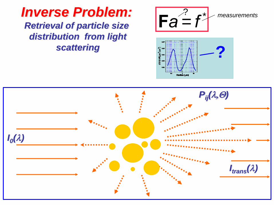
Inverse Problem: Retrieval of particle size

distribution from light

scattering

I0()

Pij()

Itrans()

?

Fa = f * measurements ?

⌢a = F

1

TC1

-1F1( )

-1

F1

TC1

-1f1

*

⌢ a = FTCf

-1F + Ca-1( )

-1

FTCf-1f * + Ca

-1 a*( )

⌢a = FTF+ gI( )

-1

FTf *

⌢a = FTC

f

-1F+gSTS( )-1

FTCf

-1f *( )

a

i

p+1= a

i

p f

i

*fi

pæ

èçç

ö

ø÷÷

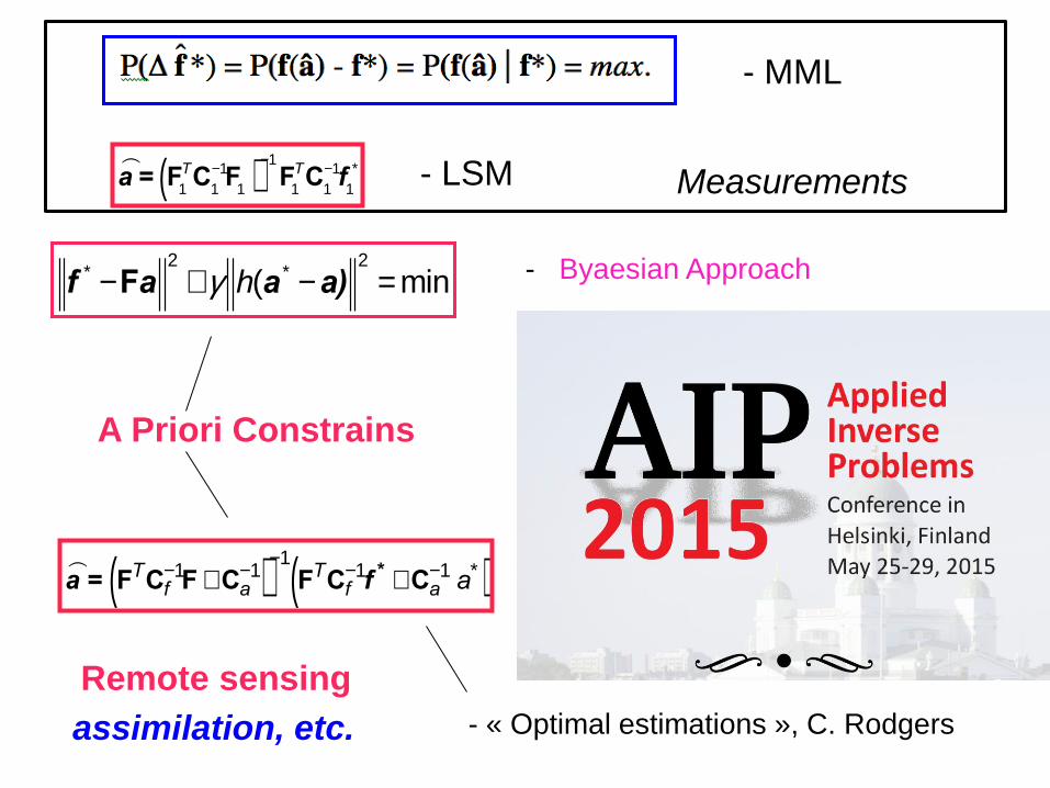
Which approach to use?

- MML

- LSM

- « Optimal estimations », C. Rodgers

- Kalman filter

- Tikhonov Regularization

- Phillips-Tikhonov-Twomey

- Twomey-Chahine

- Chahine

- Steepest Desent Method

Assimilation, 4DVR

SVD, gradient methods, etc.

⌢a = F

1

TC1

-1F1( )

-1

F1

TC1

-1f1

*

- MML

- LSM

f * -Fa

2

+g h(a* - a)2

= min - Byaesian Approach

A Priori Constrains

⌢ a = FTCf

-1F + Ca-1( )

-1

FTCf-1f * + Ca

-1 a*( )


Remote sensing

Measurements

assimilation, etc.

Base idea of inversion

f1

*

f2

*

æ

è

çç

ö

ø

÷÷

=F

11

F21

F12

F22

æ

è

çç

ö

ø

÷÷

a1

a2

æ

è

çç

ö

ø

÷÷

f1

*

f2

*

f3

*

æ

è

çççç

ö

ø

÷÷÷÷

=

F11

F12

F21

F22

F31

F32

æ

è

çççç

ö

ø

÷÷÷÷

a1

a2

æ

è

çç

ö

ø

÷÷

F

f *

a

⌢a = FTF( )

-1

FTf *

⌢a = F( )

-1

f *

- parameters of size distribution

F

f *

a

square

rectangular

Base idea of constrained

inversion

det FTF( ) ®0 FTF( )-1

- ???

What to do?


inversion


- ???

1

0

0

1

æ

èçç

ö

ø÷÷ = I - Diagonal matrix

great for inversion !!!


inversion


- ???

FTF( ) ® FTF + I( )

but det FTF + I( ) > 0 FTF + I( ) ¹ FTF( )

???


inversion


- ???

FTF( ) ® FTF +g I( )

and det FTF +g I( ) > 0 FTF +g I( ) » FTF( )

0


inversion


- ???

⌢a = FTF +g I( )

-1

FTf *

⌢a = FTF( )

-1

FTf *

0

Solution is

unique and

almost correct

!!!

⌢ a = FTCf

-1F + Ca-1( )

-1

FTCf-1f * + Ca

-1 a*( )

⌢a = FTF+ gI( )

-1

FTf *

⌢a = FTC

f

-1F+gSTS( )-1

FTCf

-1f *( )



- Kalman filter



⌢ap+1 =

⌢ap - t

pFTC-1F +g

p I( )

-1

FTC-1D lnf p - Levenberg - Marquardt

CONTENT

1. Introduction

2. Atmospheric remote sensing as an inverse problem 2.1 Interaction of radiation with the atmosphere

2.1.1 Single scattering of electromagnetic radiation

2.1.2 Multiple scattering effects

2.2 Main atmospheric components and their optical properties

2.2.1 Atmospheric gases and molecular scattering

2.2.2 Aerosols and clouds

2.2.3 Underlying surfaces: land and water

2.3 Typical inverse problems of remote sensing

2.3.1 Primary linear problems

2.3.2 Essentially non-linear problems

3. Linear system of equations 3.2 Matrix inversion solutions

3.3 Iterative linear solutions

3.4 Solutions of non-linear systems

3.5 Methods of constrained inversions, basic concept of overcoming solution instability

4. Statistical estimation concept 4.1 Solving system of equation in the presence of noise in the data

4.2 Method of Maximum Likelihood

4.3 Optimality of the Method of Maximum Likelihood

4.3.1 Cramer–Rao Inequality

4.3.2 Fisher matrix

4.3.3 Fisher definitions of information

“METHODS OF NUMERICAL INVERSION IN

ATMOSPHERIC REMOTE SENSING AND INVERSE

MODELING: AN INTRODUCTION”

5. Least Squares Method 5.1 Gaussian Distribution of Noise (Normal Central Theorem)

5.2 Formulation of the LSM as a minimization procedure

5.3 Estimation of the solution covariance matrix

5.4 Information content and its analysis

5.5 Estimations of linear functions of the retrieved parameters

6. Methods of constrained inversions 6.1 Ill-posed problem definition

6.2 Strategy of constrained inversions

6.2.1 General idea of using constraints for solving ill-posed problems

6.2.2 Smoothness a priori constraints, equations by Phillips–Tikhonov–Twomey

6.2.3 Solution constraints by means of using direct a priori estimates on unknown Kalman filter, Optimum estimations

by Rogers, Bayesian statistics approach

6.2.4 Methods for ensuring solution non-negativity and other diverse approaches 7. Including additional a priori information and Multi-Term Least Squares Method 7.1 Definition of Multi-Term LSM

7.2 Utilizing a priori estimates of unknowns

7.3 Utilizing a priori information about smoothness of the retrieved functions

7.4 Utilizing multiple a priori constraints simultaneously

7.5 Concept of statistically optimized “Multi-Pixel” Inversion

8. Optimized solution of non-linear system of equations 8.1 Optimization of solution of non-linear system in presence of noise

8.2 Gauss–Newton and Quasi-Newton iterations

8.3 Solution convergence, Levenberg–Marquardt iterations

8.4 Steepest-decent and other gradient methods

9. Limitation of “statistical estimation” optimization of inverse solution 9.1 Utilization of a priori constraints on solution non-negativity: linear regularization methods, non-linear Chahine and

Twomey–Chahine inversion procedures

9.2 Application of a priori constraints on solution non-negativity in the framework of statistical optimization formalism

9.3 Accounting for effect of “redundant observations”

10. General recommendations, remote sensing applications, the GRASP

algorithm

10.1 General recommendations for the inverse algorithm development

10.2 Satellite and ground-based atmospheric remote sensing

10.3 GRASP algorithm

10.4 Tropospheric aerosol remote sensing applications:

10.4.1 Retrieval of aerosol properties from measurements of aerosol extinction and angular singe scattering

10.4.2 Aerosol columnar properties retrieval from ground-based observations with sun-photometers

10.4.3 Aerosol columnar properties and surface reflectance retrieval from satellite multi-angular and polarimetric

observations

10.4.4 Retrieval of aerosol vertical profiles from active lidar observations

10.4.5 Enhanced retrieval of aerosol columnar and vertical properties from combined sun-photometer and lidar

ground-based observations

11. Introduction to assimilation and inverse modeling 11.1 Atmospheric chemistry transport modeling, equation of diffusion11.2 Assimilation and inverse modeling: gradient

solutions using adjoint operators

11.3 Utilization of diverse a priori constraints in assimilation and inverse modeling

11.3.1 Model forecast as an a priori estimate

11.3.2 Smoothness constraints on temporal and spatial variability of retrieved geofields

11.4 Retrieval of aerosol emission sources from remote sensing by inverse modeling

11.4.1 Retrieval of aerosol emission sources from MODIS observations by GOCART inverse modeling

11.4.2 Retrieval of aerosol emission sources from POLDER/PARASOL observations by GEOS-CHEM inverse

modeling

Multi-term LSM Multi-Pixel Solution:

av

an

an

ah

asph

aVc

abrdf ,1

abrdf ,2

abrdf ,3

abpdf

æ

è

ççççççççççççççççç

ö

ø

÷÷÷÷÷÷÷÷÷÷÷÷÷÷÷÷÷

gDW =

gD,1W

10 0 0 0 0 0 0 0 0

0 gD,2W

20 0 0 0 0 0 0 0

0 0 gD,3W

30 0 0 0 0 0 0

0 0 0 0 0 0 0 0 0 0

0 0 0 0 0 0 0 0 0 0

0 0 0 0 0 0 0 0 0 0

0 0 0 0 0 0 gD,4W

40 0 0

0 0 0 0 0 0 0 gD,5W

50 0

0 0 0 0 0 0 0 0 gD,6W

60

0 0 0 0 0 0 0 0 0 gD,7W

7

æ

è

çççççççççççççççç

ö

ø

÷÷÷÷÷÷÷÷÷÷÷÷÷÷÷÷

Sy

TSy=

Id

11

Id

12

Id

13

Id

21

Id

22

Id

23

Id

31

Id

32

Id

33

æ

è

ççççç

ö

ø

÷÷÷÷÷

0 0 0

0 0 0

0 0 0

æ

è

ççç

ö

ø

÷÷÷

0 0 0

0 0 0

0 0 0

æ

è

ççç

ö

ø

÷÷÷

0 0 0

0 0 0

0 0 0

æ

è

ççç

ö

ø

÷÷÷

Id

11

Id

12

Id

13

Id

21

Id

22

Id

23

Id

31

Id

32

Id

33

æ

è

ççççç

ö

ø

÷÷÷÷÷

0 0 0

0 0 0

0 0 0

æ

è

ççç

ö

ø

÷÷÷

0 0 0

0 0 0

0 0 0

æ

è

ççç

ö

ø

÷÷÷

0 0 0

0 0 0

0 0 0

æ

è

ççç

ö

ø

÷÷÷

Id

11

Id

12

Id

13

Id

21

Id

22

Id

23

Id

31

Id

32

Id

33

æ

è

ççççç

ö

ø

÷÷÷÷÷

æ

è

ççççççççççççççççççç

ö

ø

÷÷÷÷÷÷÷÷÷÷÷÷÷÷÷÷÷÷÷

; St

TSt=

Id

11

0 0

0 Id

11

0

0 0 Id

11

æ

è

ççççç

ö

ø

÷÷÷÷÷

Id

12

0 0

0 Id

12

0

0 0 Id

12

æ

è

ççççç

ö

ø

÷÷÷÷÷

Id

13

0 0

0 Id

13

0

0 0 Id

13

æ

è

ççççç

ö

ø

÷÷÷÷÷

Id

21

0 0

0 Id

21

0

0 0 Id

21

æ

è

ççççç

ö

ø

÷÷÷÷÷

Id

22

0 0

0 Id

22

0

0 0 Id

22

æ

è

ççççç

ö

ø

÷÷÷÷÷

Id

23

0 0

0 Id

23

0

0 0 Id

23

æ

è

ççççç

ö

ø

÷÷÷÷÷

Id

31

0 0

0 Id

31

0

0 0 Id

31

æ

è

ççççç

ö

ø

÷÷÷÷÷

Id

32

0 0

0 Id

32

0

0 0 Id

32

æ

è

ççççç

ö

ø

÷÷÷÷÷

Id

33

0 0

0 Id

33

0

0 0 Id

33

æ

è

ççççç

ö

ø

÷÷÷÷÷

æ

è


ö

ø

÷÷÷÷÷÷÷÷÷÷÷÷÷÷÷÷÷÷÷

.

Wx

= Sx

TSx; W

y= S

y

TSy; W

t= S

t

TSt;

43 parameters

Sy

TSy=

Id

11

Id

12

Id

13

Id

21

Id

22

Id

23

Id

31

Id

32

Id

33

æ

è

ççççç

ö

ø

÷÷÷÷÷

0 0 0

0 0 0

0 0 0

æ

è

ççç

ö

ø

÷÷÷

0 0 0

0 0 0

0 0 0

æ

è

ççç

ö

ø

÷÷÷

0 0 0

0 0 0

0 0 0

æ

è

ççç

ö

ø

÷÷÷

Id

11

Id

12

Id

13

Id

21

Id

22

Id

23

Id

31

Id

32

Id

33

æ

è

ççççç

ö

ø

÷÷÷÷÷

0 0 0

0 0 0

0 0 0

æ

è

ççç

ö

ø

÷÷÷

0 0 0

0 0 0

0 0 0

æ

è

ççç

ö

ø

÷÷÷

0 0 0

0 0 0

0 0 0

æ

è

ççç

ö

ø

÷÷÷

Id

11

Id

12

Id

13

Id

21

Id

22

Id

23

Id

31

Id

32

Id

33

æ

è

ççççç

ö

ø

÷÷÷÷÷

æ

è


ö

ø

÷÷÷÷÷÷÷÷÷÷÷÷÷÷÷÷÷÷÷

;

⌢a = F

1

TC1

-1F1( )

-1

F1

TC1

-1f1

*

⌢ a = FTCf

-1F + Ca-1( )

-1

FTCf-1f * + Ca

-1 a*( )

⌢a = FTF+ gI( )

-1

FTf *

⌢a = FTC

f

-1F+gSTS( )-1

FTCf

-1f *( )

a

i

p+1= a

i

p f

i

*fi

pæ

èçç

ö

ø÷÷


- MML

- LSM


- Kalman filter



- Twomey-Chahine

- Chanine

- Steepest Desent Method

f * -Fa

2

+g h(a* - a)2

= min

- Byaesian Approach

P ~ exp -1

2

(fi* -f i(a))2

iå

s2

æ

è

ç ç

ö

ø

÷ ÷

= max

Gaussian noise assumption:

P (f * - f(a)) = max

PDF(Likelihood function)

(fi* -f i(

⌢ a ))2 = min

iå

Maximum Likelihood Principle:

Least Squares Principle

LSM gives optimum solution:

sai

2 = (⌢ a i - areal )

2-Smallest !!! LSM - Optimality

noise system is redundant

noise can be accounted

2. Optimality of LSM:

1. if P (...) Gaussian, MML = MLS

Statistical Optimization

ÑY a( ) =¶Y a( )

¶ai

= 0, (i = 1,..,Na)

Y a( ) =1

2(f a( ) - f*)T C-1(f a( ) - f*) = min

f – Normal => a - Normal

<(Δg)2> = < g TΔã(g TΔã)T> =

= g TΔã(Δã)Tg = g TΔã g ≥ g TΔLSM g

- Cramer-Rao inequality

g - a characteristic linearly dependent on a (i.e. g =

g Ta, g is a vector of coefficients)

2. Shannon Information:

Fisher Information:

Information Quantity:

1.

h P ˆ C ( )( ) = -¶ 2

ln P ˆ C ( )¶ ˆ C

2

æ

è

ç ç

ö

ø

÷ ÷ ò P ˆ x ( )d ˆ x =

1

D ˆ C 2

min

h P ˆ C ( )( ) = - log2 P ˆ C ( )( )ò P ˆ C ( )dˆ x ® Nbits

Nbits- number of bits (binary digits) needed to represent the

number of distinct estimates that could have be obtained

Gauss Probability Function

P(C

)

<C>

<DC2>1/2

Nsymbols ~ 2Nbits

Information Quantity:

istina : investigation of sensitivity tendencies and · istina - : investigation of sensitivity...

Documents