Journal of Statistical Physics, Vol. 58, Nos. 5/6, 1990

Single-Cluster Monte Carlo Dynamics for the Ising Model

P. Tamayo, 1 R. C. Brower, 2 and W. Klein 3

Received July 27, 1989; revision received September 7, 1989

We present an extensive study of a new Monte Carlo acceleration algorithm introduced by Wolff for the Ising model. It differs from the Swendsen-Wang algorithm by growing and flipping single clusters at a random seed. In general, it is more efficient than Swendsen-Wang dynamics for d > 2, giving zero critical slowing down in the upper critical dimension. Monte Carlo simulations give dynamical critical exponents zw=0.33+0.05 and 0.44_+0.10 in d = 2 and 3, respectively, and numbers consistent with z w = 0 in d = 4 and mean-field theory. We present scaling arguments which indicate that the Wolff mechanism for decorrelation differs substantially from Swendsen Wang despite the apparent similarities of the two methods.

KEY W O R D S : algorithm; Wolff clusters.

Cluster acceleration; critical slowing down; Swendsen Wang algorithm; Fortuin-Kasteleyn mapping; Coniglio-Klein

1. I N T R O D U C T I O N

Considerable attention has been given in recent years to efficient Monte Carlo methods in statistical physics. Recently, Swendsen and Wang (l~ (SW) introduced a new dynamics which effectively reduces the dynamical expo- nent z and the effects of critical slowing down. This dynamics, based on the Fortuin-Kasteleyn map for site-bond percolation and the Potts model,/2'3) flips whole clusters. This increases the relaxation rate while preserving

l physics Department and Center for Polymer Studies, Boston University, Boston, Massachusetts.

2 Department of Electrical, Computer and Systems Engineering and Physics Department, Boston University, Boston, Massachusetts.

3 Physics Department and Center for Polymer Studies, Boston University, Boston, Massachusetts.

1083

0022-4715/90/0300-1083506.00/'0 �9 1990 Plenum Publishing Corporation

1084 Tarnayo et al.

detailed balance and ergodicity. Although this dynamics is useful and generalizations already exist, (4 7) there are still open questions about the dynamic universality classes (8) it introduces. ~

Here we study a single-cluster Monte Carlo algorithm introduced by Wolff (~~ for the O(N) spin models as a variation on the SW scheme for the Ising model. The main difference for the Ising case is that in each Monte Carlo step only one cluster is formed and flipped with probability 1. In the original SW algorithm all percolation clusters are formed and flipped with probability 1/2. This algorithm is an application to dynamics of the Leath cluster growth method. (1~) The single percolation cluster is grown starting from a site selected at random. The clusters formed are the same Coniglio-Klein droplets (3) used by SW dynamics, but they are sampled with an additional weight factor equal to the cluster volume. The effect of this procedure is to choose bigger clusters, which generally reduce auto- correlation times and increase the efficiency.

In this paper, we present numerical results for d = 2, 3, 4 and mean- field simulations and scaling arguments that give insight into the decorrela- tion mechanisms involved. Our main results are summarized in Table I.

2. S INGLE-CLUSTER M O N T E CARLO D Y N A M I C S

In a recent paper, Wolff considered two distinct ideas for generalizing Swendsen Wang cluster dynamics. One idea involved a new embedding scheme for the continuous spin O(N) models similar to one introduced for the ql 4 theory (6) and the other idea modified the method of updating the percolation clusters. It is this modified update procedure which we wish to study in the simplest case of the Ising model. We begin with a brief review of the basic formalism for cluster dynamics of the Ising model.

We will study relaxation rates by finite-size effects on hypercubic lattices of linear size L and volume L d in dimensions d = 2, 3, and 4. The standard Ising probability distribution is

1 I ] PI(Cri)=Zii exp K ~ ( a i ~ j - 1) (1) <i,j)

where K=J/kBT and J is the coupling constant. P~(~s) can also be expressed as a product over bonds,

1 PI(ai)= Z 1-[ [p6~,~j.~+(1--p)] (2)

( i , j )

where p = 1 - e 2K. The key step to constructing the cluster dynamics is to

Single-Cluster MC Dynamics for Ising Model 1085

consider a joint probability distribution for the Ising spins ai and site bond percolation variables nr

1 PJoint(Gi'Flij)--ZJoint 1-I [P(~ricrj, l~nij, l+(1--P)(~mj, O] (3) (i,j)

which has the property that summing over the percolation variables (n,j) gives the Ising model and summing over the Ising variables (ai) gives the so-called random percolation model,

1 PRC(nU)=~----qNc~~ [ I P [ I ( l - p ) (4)

Z - R C n 0 = I n 0 = 0

The factor qNclu~t is written correctly for a q-state Potts model, where Nclus t

is the number of clusters, although in the Ising model q-- 2. The Swendsen-Wang cluster dynamics operates on the joint model to

update the cluster distribution (or percolation variables) for fixed spins followed by an update of the spins for fixed bonds. In each percolation step the bonds are set (n o. = 1) with probability

Po = 1 - e -x(1 + ~J~ (5)

which results in the correct distribution of clusters. We define nc, the average number of clusters containing c up (or c down) spins on a lattice of size N. These distributions are analogous to the standard n~ distribution of pure q = 1 percolation, except that we do not drop the incipient infinite cluster. Hence the normalized cluster probability distribution is

P(c )= nC (6) N c l u s t

since Zc nc = Nc lus t . The SW dynamics updates all clusters drawn from this distribution, whereas WollTs dynamics consists of updating a single cluster drawn from the distribution

Iclnc P w o l f f ( c ) = ( 7 )

N

weighted by the volume of the cluster relative to the SW algorithm. In detail, the Wolff algorithm consists of the following steps:

1. Pick a site i o at random.

2. Grow a percolation cluster from i o by throwing bonds to nearest neighbors with probability Pio, j = 1 - exp[ - f l J (1 + O'i00"j)] , and continue iteratively until no new peripheral sites are generated.

1086 Tamayo et aL

3. Flip with probability one the spins in the cluster just formed, take measurements, and repeat the cycle.

The resulting dynamics is ergodic and obeys detailed balance. (1~ It differs in two respects from SW dynamics: (1) It flips a single a cluster at a time before repercolating the lattice and (2) it draws this cluster from the probability distribution Pwolff(c).

In order to compare Wolff's results with other, more conventional dynamics (Glauber, heat bath) or with SW, Wolff's Monte Carlo iteration time must be rescaled. One Wolff time step has a computational cost of the cluster size Icl, while the conventional update is proportional to the volume of the entire lattice N. Therefore, Wolff's autocorrelation time must be mul- tiplied by a factor ( [c [ ) /N, where

C2FI c (Icl)=Y~ Icl Pwol~(c)=Y N (8)

c c

By the Fortuin Kasteleyn mapping this quantity (Icl) for the random cluster model is proportional to the Ising susceptibility.

Thus, the relaxation times r~v measured in a Wolff dynamics simula- tion are rescaled according to

(Icl) , - - ~ w ( 9 ) r w - N

which with the finite-size scaling relations ( I c l ) ~ L `//v, N = L d, and r ~ L zw gives

Z w = Z'w - ( d - ~,/v) (10)

This Zw is the correct parameter to compare with the dynamical exponents of Swendsen-Wang, Zsw.

3. A N A L Y S I S A N D N U M E R I C A L RESULTS

In our computer simulations, we accumulate measurements of the internal energy, magnetization, and susceptibility at every time step. To estimate r~v, we compute the time autocorrelation function over samples of at least 3 x 10 5 steps. The autocorrelation function being considered

(A(O) A ( t ) ) - ( A ) 2 C( t )= ( A ) 2 - ( A ) 2 (11)

where the average is over the sampling time and A is the energy or suscep- tibility. T~v is determined from a linear fit of log C(t) to t in the region in which the long-time single exponential decay is seen.

Sing le -C lus te r M C Dynamics for Ising M o d e l

Table I a

1087

d = 2 d = 3 d = 4 Mean-field

7 1.75 1.25 1 1

v 1 0.629 �89 �89 d - y/v 0.25 1.01 2 2

Z~v 0.58 _+ 0.05 1.45 _+ 0.10 1.95 4- 0.15 1.90 _+ 0.15

z w 0.33 + 0.05 0.44 + 0.10 - 0 . 0 5 + 0.15 - 0 . 1 0 _+ 0.15

Zsw 0.35 0.75 - - 1

a The first three rows give the static exponents 7, v, and the rescaling shift. The next two rows

give our measured Wolf f exponents and its shifted values: z w = Z'w - ( d - 7 / v ) . The last row

gives the S w e n d s e n - W a n g exponents. {n

Statistical fluctuations in C(t) lead to errors in the calculation of r~v.(n 15) To estimate those errors, we split the data sample into several groups and recomputed r;v for each group. Each group is much longer than r~v. The error is computed using standard error analysis techniques. Values of r;v are computed for different lattice sizes at the critical point for the infinite lattice and an estimate for Z~v is obtained by finite-size scaling,

-c~ ~ ~v ~ L~v (12)

Fig. 1.

1.5

1.0

0.5

I . . . . I . . . . I '- ' I ' ' '

SW

0.0

1 2

Wolff ]

,, 2 t 3 4 5

d Dynamica l critical exponents z versus dimensional i ty for S w e n d s e n - W a n g and Wolf f

algorithms.

1088 Tamayo e t al.

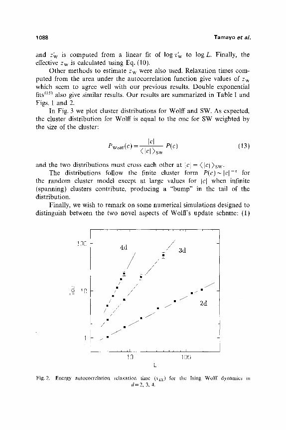
and Z~v is computed from a linear fit of log rw to log L. Finally, the effective Zw is calculated using Eq. (10).

Other methods to estimate Zw were also used. Relaxation times com- puted from the area under the autocorrelation function give values of Zw which seem to agree well with our previous results. Double exponential fits (15) also give similar results. Our results are summarized in Table I and Figs. 1 and 2.

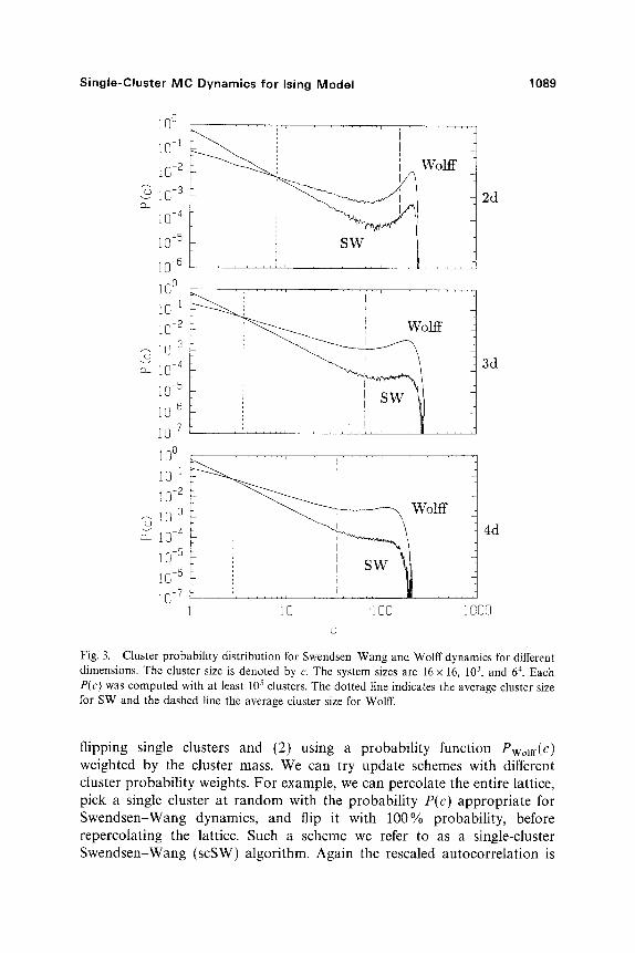
In Fig. 3 we plot cluster distributions for Wolff and SW. As expected, the cluster distribution for Wolff is equal to the one for SW weighted by the size of the cluster:

Icl Pwo]ff(c) - - P(c) (13) <lcl>sw

and the two distributions must cross each other at tc[ = (Icb)sw. The distributions follow the finite cluster form P ( c ) ~ l c l ~ for

the random cluster model except at large values for Ic[ when infinite (spanning) clusters contribute, producing a "bump" in the tail of the distribution.

Finally, we wish to remark on some numerical simulations designed to distinguish between the two novel aspects of Wolff's update scheme: (1)

100

o 10

4d

/ / I

/

/ / /

/ / �9

�9 /

// / / " / f

�9 / / / / /

. J

/// / 3d

J �9 J

J 2d

i , n n n , h i i n i a , i n n l

lO lOS L

Fig. 2. Energy autocorrelation relaxation time (tEE) for the Ising Wolff dynamics in d=2, 3, 4.

Single-Cluster M e Dynamics for Ising Model 1089

lO ~

10 1

!0 -2

l O - 3

10 -4

10 -5

10 -6

!0 o

I0 q

10 ~

~ l O 3

m l O 10-5

1@ ~ 10-7

10 0

lO -1

i@ -z !@ -3

o

i@ -4

1@ 5

10 6

10 _7

. . . . ! . . . . . . . . . . . i . . . . . . . - i I W o l f f

i

! S W i . . . . . . . . . S w .... 1 . . . . . .

i . . . . . . I . . . . . . .

. . . . . . . . . . . S W it ' ,

10 1@@

2d

3d

4d

1000

Fig. 3. Cluster probability distribution for Swendsen Wang and Wolff dynamics for different dimensions. The cluster size is denoted by c. The system sizes are 16 x 16, 10 3, and 6 4. Each P(c) was computed with at least 10 s clusters. The dotted line indicates the average cluster size for SW and the dashed line the average cluster size for Wolff.

flipping single clusters and (2) using a probability function Pwom-(c) weighted by the cluster mass. We can try update schemes with different cluster probability weights. For example, we can percolate the entire lattice, pick a single cluster at random with the probability P(c) appropriate for Swendsen-Wang dynamics, and flip it with 100% probability, before repercolating the lattice. Such a scheme we refer to as a single-cluster Swendsen-Wang (scSW) algorithm. Again the rescaled autocorrelation is

1090 Tamayo et' al.

defined by rescaling the measured r'scsw "~L z;~ by a factor <]c] >sw/N, where

<lcl>sw : ~ Icl n~ N (14) Nclust Nclust

Here <lcl>sw scales as L ~ so that the rescaled rscsw gives Zsosw = z'scsw - d.

It should be emphasized that, unlike Wolff's algorithm, there may be no way of actually finding these single clusters in O(Nclust) operations. Nonetheless, choosing single clusters from various probability distributions can help in analyzing the role of cluster sizes. Our present simulations give A~sw -- 0.17 _+ 0.10 and 0.45 _+0.15 for d = 2 and 3, respectively. Since the intervening percolation steps should act to further decorrelate clusters, the fact that our results are consistent with A~sw ~<Zsw might have been anticipated. Further interpretations should await more accurate data across a broader range of lattices sizes and probability distributions.

4. CONCLUSIONS

The data presented in the previous section demonstrate clearly that the Wolff algorithm has smaller decorrelation times in three and four dimensions than SW, and correspondingly smaller exponents (i.e., Z w < ZSW ).

In two dimensions, the exponents are equal (Zw -Zsw) within error bars. Morever, there may be finite-size effects visible in the curvature of the d-- 2 data of Fig. 2, which would imply a smaller Zw asymptotically.

To understand why Wolff dynamics can be faster than SW, we have measured the cluster size distribution for the SW and Wolff algorithms. It is obvious from Fig. 3 that one reason that the Wolff algorithm is more efficient than SW is that the mean size of the clusters flipped is significantly larger. Specifically, the method of choosing the Wolff clusters, i.e., choosing a cluster with a probability proportional to the number of spins in the cluster, is equivalent to multiplying the SW cluster distribution by the mean cluster size. For large clusters the size of the correlation length ~ thus results in a maximum of ~/v incipient infinite clusters per Monte Carlo time step rather than the one incipient infinite cluster per time step in SW. This restriction to one incipient infinite cluster per time step in SW is a consequence of the percolation definition of the flipped clusters.(16'1'3)

To understand the Wolff algorithm and how it differs from SW, we must consider the dynamics of the incipient infinite clusters and how the Wolff algorithm employs them to eliminate the correlations. In the SW algorithm we have argued (9) that the mechanism of domain wall diffusion,

Single-Cluster MC Dynamics for Ising Model 1091

which dominates the decorrelation mechanism in the Glauber algorithm, is retained. If the Wolff algorithm is using the incipient infinite cluster of size

to elimiate correlated domains, then it cannot eliminate them by domain wall diffusion. An alternate mechanism is the uniform thinning of large correlated domains in a (roughly) uniform manner.

If the incipient infinite clusters are independent, or correlated over a finite time, then one could describe the "thinning" decorrelation process in the Wolff algorithm as a directed walk in magnetization space with a step size equal to the mass of the incipient infinite cluster ~a-~. Here ~ is the correlation length,/~ is the order parameter exponent, (~6,3) v is the correla- tion length exponent, {16'3) and d is the dimension of space. To eliminate a domain of mass ~d requires ~d/~d-~/v = ~/v steps and hence a time which scales as ~2B/v.

For d~>4 the incipient infinite clusters are independent. This can be seen from the following argument. In infinite dimensions incipient infinite clusters with fractal dimension 4 will not interfere with each other. There- fore, one expects no correlation between large clusters, since they do not "see each other." This leads to a z~ ~ ~2B/~ and a renormalized Zw =0. Since Zw for d~> 4 should be the same as the infinite-dimension value, we expect Zw = 0 in d = 4. This is consistent with the data (see Table I).

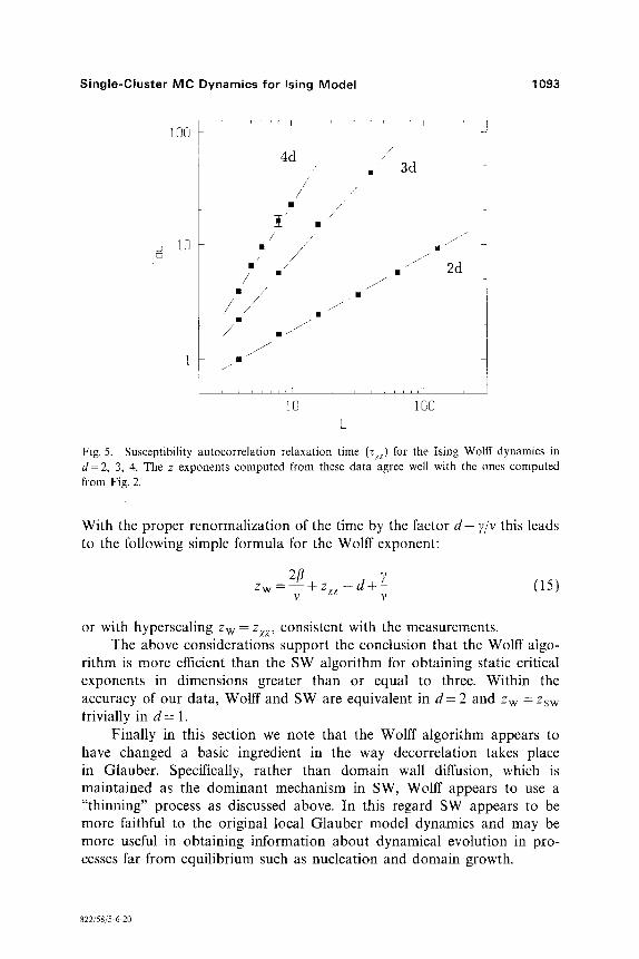
To support this argument, we have measured the time-dependent susceptibility-susceptibility correlation function (ZX) (Fig. 5). Since the mean cluster size is equivalent to the susceptibility, (m3) (XZ) will be proportional to the cluster-cluster correlations for clusters the size of 4. In d = 4 , <ZZ) decays exponentially, leading to the conclusion that there are only finite time correlations and that the clusters can be treated as independent.

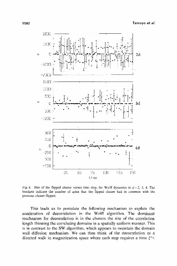
In addition, we have plotted in Fig. 4 the size of the "flipped cluster" for each unrenormalized time step. The y axis is the size of the cluster, with the sign denoting the direction of the flip, and the x axis is the time where one time unit corresponds to one cluster flip. The brackets about some of the points in the figure represent the number of spins that a particular cluster had in common with the previous cluster flipped in the opposite direction. This plot, consistent with Fig. 5, shows almost no correlation between large clusters in d = 4.

We have made the same cluster size-time plots for d = 2 and 3. The difference is striking. Clearly there is considerably more correlation between large clusters in 2 and 3 dimensions than there is in 4. This is supported by the measurement of (TJ~) in d = 2 and 3. As can be seen from Fig. 5, the relaxation time scales with the system size. Fitting the data to exponential decay, we extract a relaxation time that diverges as ~z~, where zzz = Zw within the accuracy of the data.

1092 Tamayo e t al,

2000

1000

0

iO00

-2000

1500

i000

500

0

-500

1000

!!!T.TT !! W.ii:.i! i.i~ii �9

l

T! TT. m ' i~.t "ii ';..

i; i ~iiiii i i

:

T I TT TTTT !T l- �9 T �9 " " � 9 1 4 9 1 4 9 �9 " �9 �9 �9 �9 . . ~, . . " ~ I I I ' I ' i ' I '~T 11"

�9 . T . . �9 TT. { . . . , T i �9 ae

2d

3d

(O

500

250

0

-250

-500

-750

.! 1 " i . �9 .

�9 "" v �9 I T

i i

25 50 75 100 125 t ime

4d

150

Fig. 4. Size of the flipped cluster versus time step, for Wolff dynamics in d= 2, 3, 4. The brackets indicate the number of spins that the flipped cluster had in common with the previous cluster flipped.

This leads us to pos tu la te the fol lowing mechan i sm to explain the acce le ra t ion of decor re la t ion in the Wolff a lgor i thm. The d o m i n a n t mechan i sm for decor re la t ion is in the clusters the size of the cor re la t ion length th inning the corre la t ing domains in a spat ia l ly uniform manner . This is in con t ras t to the SW algor i thm, which appears to ma in ta in the d o m a i n wall diffusion mechanism. We can then th ink of the deeor re la t ion as a d i rec ted walk in magne t i za t ion space where each step requires a t ime ~z~.

Single-Cluster MC Dynamics for Ising Modei 1093

i00

10

4d /

i

/

/ i /

�9 /

/

/ . / �9 / J "

J

,1

[]

J J

i

3d

m

..... 2d

, , E , , , 1 [ , , , L E , i r l

10 i00

Fig. 5. Susceptibility autocorrelation relaxation time (zxz) for the Ising Wolff dynamics in d= 2, 3, 4. The z exponents computed from these data agree well with the ones computed from Fig. 2.

With the proper renormalization of the time by the factor d - 7/v this leads to the following simple formula for the Wolff exponent:

Zw = - - + zx• - d + Z (15) V V

or with hyperscaling Zw = zx~, consistent with the measurements. The above considerations support the conclusion that the Wolff algo-

rithm is more efficient than the SW algorithm for obtaining static critical exponents in dimensions greater than or equal to three. Within �9 the accuracy of our data, Wolff and SW are equivalent in d = 2 and Zw -- Zsw trivially in d = 1.

Finally in this section we note that the Wolff algorithm appears to have changed a basic ingredient in the way decorrelation takes place in Glauber. Specifically, rather than domain wall diffusion, which is maintained as the dominant mechanism in SW, Wolff appears to use a "thinning" process as discussed above. In this regard SW appears to be more faithful to the original local Glauber model dynamics and may be more useful in obtaining information about dynamical evolution in pro- cesses far from equilibrium such as nucleation and domain growth.

822/58/5-6-20

1094 Tamayo et al.

A C K N O W L E D G M E N T S

We would like to acknowledge many useful conversa t ions with A. Sokal , A. Fer renberg , T. Ray, R. Swendsen, R. Edwards , H. Gould , A. Conigl io , N. Jan, R. Giles, and D. Stauffer. We also thank J. Leao from the Physics C o m p u t i n g Faci l i ty and Chip Cole from the Academic C o m p u t i n g Center at Bos ton Universi ty. This project was suppor t ed in par t by a g ran t from the Office of N a v a l Research.

R E F E R E N C E S

1. R. Swendsen and J. S. Wang, Phys. Rev. Lett. 58:86 (1987). 2. C. M. Fortuin and P. W. Kasteleyn, Physica 57:536 (1972). 3. A. Coniglio and W. Klein, J. Phys. A 13:2775 (1980). 4. F. Niedermayer, Phys. Rev. Lett. 61:2026 (1988). 5. R. G. Edwards and A. D. Sokal, Phys. Rev. D 38:2009 (1988); A. Sokal, Monte Carlo

methods in statistical mechanics: Foundations and new algorithms, Lecture Notes. 6. R. Brower and P. Tamayo, Phys. Rev. Lett. 62:1087 (1989). 7. T. Ray, P. Tamayo, and W. Klein, Phys. Rev. A 39:5949 (1989). 8. P. C. Hohenberg and B. Halperin, Rev. Mod. Phys. 49:435 (1977). 9. W. Klein, T. Ray, and P. Tamayo, Phys. Rev. Lett. 62:163 (1989).

10. U. Wolff, Phys. Rev. Lett. 62:361 (1989). 11. P. L. Leath, Phys. Rev. B 14:5046 (1976). 12. K. Binder, ed., Monte Carlo Methods in Statistical Physics (Springer-Verlag, 1979). 13. H. Gould and J. Tobochnik, Computer Simulation Methods (Addison-Wesley, 1988). 14. E. Stoll, K. Binder, and T. Schneider, Phys. Rev. B 8:3266 (1973). 15. S. Tang and D. P. Landau, Phys. Rev. B 36:567 (1987). 16. T. Ray and W. Klein, J. Star. Phys. 53:773 (1988).