is the cnmssm more credible than the cmssm?
TRANSCRIPT

Is the CNMSSM more credible than the CMSSM?
Andrew Fowlie∗
National Institute of Chemical Physics and Biophysics,
Ravala 10, Tallinn 10143, Estonia
(Dated: November 9, 2021)
AbstractWith Bayesian statistics, we investigate the full parameter space of the constrained “next-to-
minimal” supersymmetric Standard Model (CNMSSM) with naturalness priors, which were derived
in a previous work. In the past, most Bayesian analyses of the CNMSSM ignored naturalness of the
electroweak (EW) scale by making prejudicial assumptions for parameters defined at the EW scale.
We test the CNMSSM against the CMSSM with Bayesian evidence, which, with naturalness priors,
incorporates a penalty for fine-tuning of the EW scale. With the evidence, we measure credibility
with respect to all measurements, including the EW scale and LHC direct searches. We find that
the evidence in favor of the CNMSSM versus the CMSSM is “positive” to “strong” but that if one
ignores the µ-problem, the evidence is “barely worth mentioning” to “positive.” The µ-problem
significantly influences our findings. Unless one considers the µ-problem, the evidence in favor of
the CNMSSM versus the CMSSM is at best “positive,” which is two grades below “very strong.” We,
furthermore, identify the most probable regions of the CMSSM and CNMSSM parameter spaces
and examine prospects for future discovery at hadron colliders.
1
arX
iv:1
407.
7534
v2 [
hep-
ph]
10
Nov
201
4

I. INTRODUCTION
The Standard Model (SM) contains a well-known “hierarchy problem” [1, 2]. The problem
has two puzzling facets:(1) why is the magnitude of the electroweak (EW) scale much less
than the Planck scale, MZ � MP? and (2) why is the EW scale stable despite massive
quadratic corrections, ∆M2Z ∼M2
P?
Weak-scale supersymmetry (SUSY) [3–5] solves the “stability” aspect of the hierarchy
problem by positing a “mirror” of the SM fields with spins differing by one-half. Massive
quadratic corrections from scalars cancel with identical corrections from fermions (see e.g., [6–
8]). Because residual corrections are similar to the SUSY breaking scale, ∆M2Z ∼ M2
SUSY,
the SUSY breaking scale should be close to the EW scale [9, 10].
Minimal SUSY, however, aggravates the “magnitude” aspect of the hierarchy problem.
“Supersymmetrizing” the SM with minimal field content, the EW scale is function of a SUSY
breaking scale, mHu , and a SUSY preserving scale, µ,
1
2M2
Z ' −µ2 −m2Hu|EW (1)
where µ is protected from massive quadratic corrections by a supersymmetric non-
renormalization theorem but is unrelated to a symmetry breaking scale, whereas the
SUSY breaking up-type Higgs mass, m2Hu
, receives massive radiative corrections proportional
to the supersymmetric top (stop) mass, ∆m2Hu∼ m2
t.1
This is the “µ-problem” [11]. It would be preferable if the EW scale were a function
of only the SUSY breaking scale so that explaining the magnitude of the EW scale would
be equivalent to explaining the magnitude of the SUSY breaking scale, which presumably
originates from a hidden sector. This is realized with an extra gauge singlet superfield [12];
the µ-parameter is generated spontaneously by SUSY breaking parameters.
This picture is, however, spoiled by experimental results from the Large Hadron Collider
(LHC) that suggest that the SUSY breaking scale is not close to the EW scale, including
the measurement of the Higgs mass mh ' 126GeV [13–15] and the absence of SUSY in
ATLAS [16] and CMS [17] searches. In minimal supersymmetric models (see e.g., [6]),
m2h ' cos2 2βM2
Z + ∆m2h, (2)
1 In Eq. (1), m2Hu|EW is negative. The quantity m2
Huis a parameter in the soft-breaking Lagrangian; it is
not the square of a parameter.
2

where tan β = 〈Hu〉/〈Hd〉 and the loop-corrections
∆m2h =
3
4π2cos2 α y2tm
2t ln
(m2t
m2t
). (3)
Because mh ' 126GeV, the loop-corrections, ∆mh, and thus stop masses, mt, must be
appreciable. Heavy stops “poison” the prediction for the EW scale in Eq. (1). By contributing
radiatively to m2Hu
, heavy stops result in −m2Hu�M2
Z .
The separation between the SUSY breaking scale and the EW scale in “next-to-minimal”
models, however, could be smaller than that in minimal models. In “next-to-minimal” models
(see e.g., [18, 19]), there is an additional tree-level contribution to the Higgs mass;
m2h ' cos2 2βM2
Z + λ2v2 sin2 2β + ∆m2h, (4)
where λ originates from a cubic interaction in the superpotential and v ' 174GeV. The loop-
corrections and thus stop masses in “next-to-minimal” models could be smaller than those in
minimal models, because of the extra tree-level contribution to the Higgs mass [20–26].
Let us examine both facets of the hierarchy problem, including the µ-problem, in a
“next-to-minimal” and in a minimal SUSY model in light of LHC results. With Bayesian
statistics, we will calculate whether a “next-to-minimal” model is more credible than a
minimal model, and if so, we will quantify its superiority with Bayesian evidence. With the
Bayesian posterior density, we will find the most probable regions of their parameter spaces
in light of experimental data and Bayesian naturalness considerations. We will show that
the µ-problem significantly influences our findings.
II. MODELS
We consider two models, the CMSSM and the CNMSSM, defined below to clarify our
parameterization. Our notation is similar to that of Ref. [6].
A. CMSSM
Our minimal model is the Constrained Minimal Supersymmetric SM (CMSSM) [27–29].
The model’s superpotential is
WMSSM = uyuQHu − dydQHd − eyeLHd + µHuHd. (5)
3

The model’s soft-breaking Lagrangian at the Grand Unification (GUT) scale is
LMSSMsoft =− 1
2m1/2
(bb+ WW + gg + c.c.
)−m2
0
(Q†Q+ L†L+ ˜u˜u† + ˜d ˜d† + ˜e˜e† +H∗uHu +H∗dHd
)− A0
(˜uyuQHu − ˜dydQHd − ˜eyeQHd + c.c.
)− bHuHd + c.c.
(6)
Thus the model is described by five parameters: four SUSY breaking parameters,
m1/2, m0, A0, and b, (7)
and the µ-parameter in the superpotential.2 In a phenomenological parameterization of the
CMSSM, b and µ2 are traded for tan β and MZ via EW symmetry breaking conditions.
The CMSSM contains two Higgs doublets with eight real degrees of freedom. In EW
symmetry breaking, the W - and Z-bosons “eat” three degrees of freedom from the Higgs
doublets. The five remaining degrees of freedom are equivalent to five physical Higgs bosons:
a light SM-like Higgs, h, a heavy neutral Higgs, H, a heavy charged Higgs, H±, and a neutral
CP-odd Higgs, A.
After EW symmetry breaking, off-diagonal masses “mix” bino, wino and Higgsino fields
into mass eigenstates called “neutralinos,” χ0. The phenomenology of the four neutralinos is
rich. If the lightest neutralino is the lightest supersymmetric particle (LSP) and if it cannot
decay to SM particles, dark matter (DM) could be the lightest neutralino (see e.g., [30]).
B. CNMSSM
Our “next-to-minimal” model is the Constrained “Next-to-minimal” Supersymmetric SM
(CNMSSM or C(M+1)SSM) with an extra gauge singlet superfield, S (see e.g., [18, 19]). The
superpotential contains extra terms with the singlet superfield;
WNMSSM =WMSSM|µ=0 + λSHuHd +1
3κS3. (8)
The µ-term that was permitted in the MSSM, a singlet bilinear and a singlet tadpole are
forbidden by a discrete Z3 symmetry or classical scale invariance. Because the superpotential2 The CMSSM is also described by Yukawa couplings in the superpotential. We consider the Yukawa
couplings in the CMSSM and CNMSSM as “nuisance” parameters: model parameters that are not of
particular interest.
4

is protected by a non-renormalization theorem, such terms cannot be generated by radiative
corrections.
The model’s soft-breaking Lagrangian at the GUT scale is
LNMSSMsoft =LMSSM
soft |b=0
−m2SS∗S
− A0
(λSHuHd −
1
3κS3 + c.c.
).
(9)
Bilinear and tadpole, tS, terms are forbidden by a discrete Z3 symmetry. A tadpole term
would be problematical [31]; if S were a singlet under all symmetries, radiative corrections
from any heavy fields would result in t�M3Z . Each trilinear coupling in the soft-breaking
Lagrangian is proportional to the corresponding trilinear coupling in the superpotential in
analogy with the MSSM in which e.g., au = Auyu.
If the scalar field S obtains a non-zero vacuum expectation value (VEV), the discrete Z3
symmetry and classical scale invariance are spontaneously broken, but SUSY is preserved
as the vacuum expectation of the scalar potential remains zero, and an effective µ-term
µeff = λ〈S〉HuHd is spontaneously generated in Eq. (8). The magnitude of 〈S〉 is determined
from a symmetry breaking constraint, ∂V /∂S = 0.
That the discrete Z3 symmetry is spontaneously broken is problematic. During spontaneous
symmetry breaking, topologically stable field configurations, known as domain walls, would
form at the spatial boundaries of degenerate vacua. The spatial variation in the field between
the degenerate vacua represents a considerable energy density. Because domain walls could
dominate the energy density of the Universe, domain walls could spoil successful predictions
of inflation and nucleosynthesis.
The NMSSM’s additional gauge singlet superfield modifies the neutralino and Higgs
sectors of the MSSM with two on-shell fermionic and two on-shell scalar degrees of freedom.
The two scalar degrees of freedom result in two extra Higgs bosons and alter the mixing
angles between the physical Higgs bosons and the gauge eigenstates. In general, the NMSSM
Higgs-sector violates CP-symmetry at tree-level. If, however, complex phases are forbidden,
the Higgs sector respects CP. There are three CP-even neutral Higgs bosons, H1, H2 and
H3; two CP-odd neutral Higgs bosons, A1 and A2; and one charged Higgs boson, H±. Unlike
in the CMSSM, in the CNMSSM several Higgs bosons could be near the EW scale. The
observed Higgs boson need not be the lightest CP-even neutral Higgs boson in the CNMSSM.
5
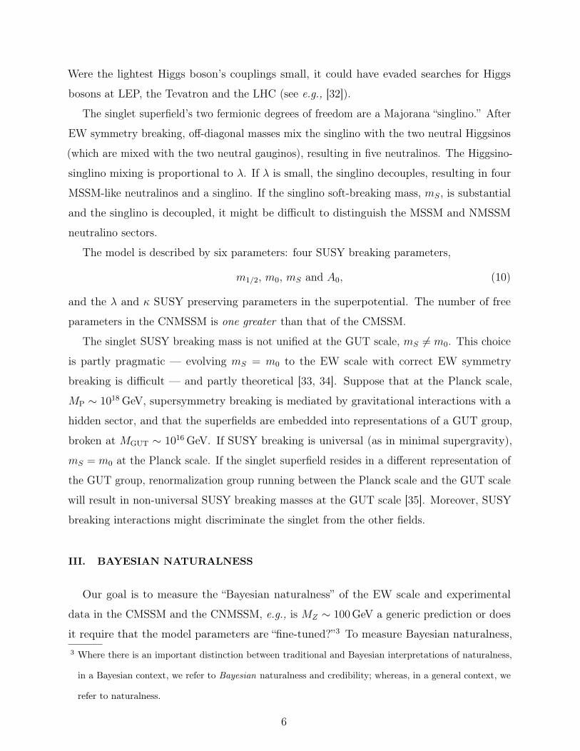
Were the lightest Higgs boson’s couplings small, it could have evaded searches for Higgs
bosons at LEP, the Tevatron and the LHC (see e.g., [32]).
The singlet superfield’s two fermionic degrees of freedom are a Majorana “singlino.” After
EW symmetry breaking, off-diagonal masses mix the singlino with the two neutral Higgsinos
(which are mixed with the two neutral gauginos), resulting in five neutralinos. The Higgsino-
singlino mixing is proportional to λ. If λ is small, the singlino decouples, resulting in four
MSSM-like neutralinos and a singlino. If the singlino soft-breaking mass, mS, is substantial
and the singlino is decoupled, it might be difficult to distinguish the MSSM and NMSSM
neutralino sectors.
The model is described by six parameters: four SUSY breaking parameters,
m1/2, m0, mS and A0, (10)
and the λ and κ SUSY preserving parameters in the superpotential. The number of free
parameters in the CNMSSM is one greater than that of the CMSSM.
The singlet SUSY breaking mass is not unified at the GUT scale, mS 6= m0. This choice
is partly pragmatic — evolving mS = m0 to the EW scale with correct EW symmetry
breaking is difficult — and partly theoretical [33, 34]. Suppose that at the Planck scale,
MP ∼ 1018 GeV, supersymmetry breaking is mediated by gravitational interactions with a
hidden sector, and that the superfields are embedded into representations of a GUT group,
broken at MGUT ∼ 1016 GeV. If SUSY breaking is universal (as in minimal supergravity),
mS = m0 at the Planck scale. If the singlet superfield resides in a different representation of
the GUT group, renormalization group running between the Planck scale and the GUT scale
will result in non-universal SUSY breaking masses at the GUT scale [35]. Moreover, SUSY
breaking interactions might discriminate the singlet from the other fields.
III. BAYESIAN NATURALNESS
Our goal is to measure the “Bayesian naturalness” of the EW scale and experimental
data in the CMSSM and the CNMSSM, e.g., is MZ ∼ 100GeV a generic prediction or does
it require that the model parameters are “fine-tuned?”3 To measure Bayesian naturalness,3 Where there is an important distinction between traditional and Bayesian interpretations of naturalness,
in a Bayesian context, we refer to Bayesian naturalness and credibility; whereas, in a general context, we
refer to naturalness.
6

we will utilize Bayesian statistics. Ref. [36–39] argued that naturalness and fine-tuning
arguments are Bayesian in nature. Let us briefly recapitulate this argument (see e.g., [39]).
In Bayesian statistics, probability is a numerical measure of our degree of belief in a
proposition, rather than the frequency at which outcomes occur in repeated trials. We
must calculate the probability that our model is correct, given experimental data, e.g., the
measured EW scale. By Bayes’ theorem, we may write this probability as a function of
the Bayesian evidence, Z ≡ p(data |model); our belief in the model prior to seeing the
experimental data, p(model); and an unknown normalization constant, p(data);
p(model | data) =p(data |model)× p(model)
p(data). (11)
To eliminate the normalization constant in Eq. (11),4 we consider the ratio of probabilities
for our two models, the CMSSM and the CNMSSM;p(CMSSM | data)
p(CNMSSM | data)︸ ︷︷ ︸Posterior odds, θ′
=p(data |CMSSM)
p(data |CNMSSM)︸ ︷︷ ︸Bayes-factor, B
× p(CMSSM)
p(CNMSSM)︸ ︷︷ ︸Prior odds, θ
. (13)
Our prior odds, θ, is a numerical measure of our relative belief in the CMSSM over the
CNMSSM, prior to seeing the experimental data. The Bayes-factor, B, updates our prior
odds, θ, with the experimental data, resulting in our posterior odds, θ′. Our posterior odds is
a numerical measure of our relative belief in the CMSSM over the CNMSSM, after seeing
the experimental data. The Bayes-factor is the ratio of the models’ evidences.
If the Bayes-factor is greater than (less than) one, the model in the numerator (denomi-
nator) is favored. The interpretation of Bayes-factors is somewhat subjective, though we
have chosen the Jeffreys’ scale, Table I, to ascribe qualitative meanings to Bayes-factors. If a
Bayes-factor is sufficiently large, all investigators will conclude that a particular model is
favorable, regardless of their prior odds for the models.
The Bayes-factor quantitatively incorporates a Bayesian interpretation of “naturalness” [9,
10, 42]. Consider the evidence Z = p(data |model) a function of the data normalized to
unity [43]. Natural models “spend” their probability mass near the obtained data, i.e., a large
fraction of their parameter space agrees with the data. Complicated models squander their4 Alternatively, we could assume that there exists a finite set of alternative models one of which is true, in
which case we could calculate the normalization constant;
p(data) =∑i
p(data |modeli)× p(modeli). (12)
7

Grade Bayes-factor, B Preference for model in numerator
0 B ≤ 1 Negative
1 1 < B ≤ 3 Barely worth mentioning
2 3 < B ≤ 20 Positive
3 20 < B ≤ 150 Strong
4 B > 150 Very strong
Table I: The Jeffreys’ scale for interpreting Bayes-factors [40, 41], which are ratios of evidences.
We assume that the favored model is in the numerator, though this could be readily inverted.
probability mass away from the obtained data. For example, the SM is unnatural because
its generic prediction for the EW scale is MZ ∼MP. See e.g., Ref. [39] for elaboration.
With Bayes’ theorem, it can be readily shown that the evidence is an integral over
the likelihood — the probability of obtaining data given a particular point in a model’s
parameter space, L(~x) ≡ p(data | ~x,model) — times the prior — our prior belief in the
model’s parameter space, π(~x) ≡ p(~x |model);
Z =
∫L(~x)× π(~x)
∏dx. (14)
A. Bayesian posterior
A probability density function (PDF) for the model’s parameter space in light of the
experimental data — the posterior — is a by-product of the calculation of the Bayesian
evidence. By Bayes’ theorem, the posterior density for a point ~x in a model’s parameter
space is
p(~x |model, data) =p(data | ~x, model)× p(~x |model)
p(data |model)
≡ L(~x)× π(~x)
Z .
(15)
The evidence, Z, is merely a normalization constant in this instance. The likelihood, L,updates our prior belief with experimental data, resulting in our posterior.
The posterior in Eq. (15) is a PDF of all of the model’s parameters. To find the PDF for
8

e.g., two of the model’s parameters, we “marginalize” the posterior;
p(x1, x2 |model, data) =
∫p(~x |model, data) dx3dx4 · · · (16)
Marginalization incorporates “fine-tuning.” If for fixed (x1, x2), few combinations of x3, x4, . . .
result in an appreciable posterior density, p(~x |model, data), the marginalized posterior at
(x1, x2) will be small. For further details, see e.g., Ref. [44].
IV. METHODOLOGY
Our calculation of the evidence from Eq. (14) requires two ingredients: our priors,
which contain our prior beliefs about the model’s parameter space, and our likelihood
function, which contains relevant experimental data. We supply our priors and our likelihood
functions to the nested sampling algorithm with importance sampling implemented in
(Py)MultiNest-3.4 [45, 46], which returns the models’ Bayesian evidences and posterior
PDFs.
This investigation is similar to that in Ref. [36, 37, 39, 47–49], in which the posterior PDF
is calculated for the CMSSM with naturalness priors, Ref. [50, 51], in which the posterior
PDF is calculated for the CNMSSM but without naturalness priors, and Ref. [24], in which a
naturalness prior is calculated for the CNMSSM. The posterior PDF for the CNMSSM with
naturalness priors and the Bayes-factor for the CNMSSM versus the CMSSM are, however,
absent in the literature.
A. Likelihood function
Our likelihood function includes data from relevant laboratory measurements:
(1) The measured Z-boson mass, MZ = 91.1876GeV [13], with a Dirac likelihood function.
(2) Measurements and searches for Higgs bosons at LEP, the Tevatron and the LHC
with a 2GeV theoretical uncertainty in the Higgs mass [52]. The likelihood is from
HiggsSignals-1.2.0 [53–57] with the “latest results” dataset (see Fig. 2 of Ref. [53]
for a summary of the experimental data).
9

HiggsSignals-1.2.0 confronts the whole Higgs sector — all Higgs bosons — with
data. We do not need to separately consider different interpretations of the SM-like
Higgs boson in the CNMSSM.
(3) The ATLAS-CONF-2013-047 [16] 0 leptons + 2-6 jets + MET search with a hard-cut on
the (m0, m1/2) 95% confidence limit. The (m0, m1/2) confidence limit is approximately
independent of (A0, tan β) [58–60] and the extra CNMSSM singlet superfield [51].
(4) The magnetic moment of the muon calculated with SuperIso-3.3 [61–63].
(5) B-physics rare decays — BR(Bs → µµ), BR(Bs → Xsγ) and BR(Bu → τν) —
calculated with SuperIso-3.3.
For the numerical values of the constraints, see Table II. We calculate mass spectra for the
CMSSM and CNMSSM with SOFTSUSY-3.4.1 [64, 65]. Our codes for the CNMSSM are
consistent with our codes for the CMSSM. Unfortunately, the precise Higgs mass calculation
in FeynHiggs-2.10.0 [66–69] is unavailable in the CNMSSM. We omit observables that we
cannot consistently calculate, e.g., EW precision observables.
We exclude DM experiments from our likelihood, e.g., the Planck measurement of the
DM density from the cosmic microwave background (CMB) [70] and the LUX search for
DM with an underground detector [71], because fine-tuning related to DM might cloud our
understanding of the fine-tuning of the EW scale. If we were to include DM experiments, we
would invoke particular DM annihilation mechanisms by fine-tuning the supersymmetric par-
ticle (sparticle) masses and the mixing angles between mass and gauge eigenstates. Including
DM experiments would, furthermore, require additional assumptions and uncertainties (see
e.g., [72]).
B. Priors
We pick “naturalness priors” [24, 36–39, 47–49] for the model parameters. That is, we
pick priors for the model parameters in the soft-breaking Lagrangian and superpotential at
the GUT scale and transform to parameters at the EW scale e.g., tan β, obtained after EW
symmetry breaking, with the appropriate Jacobian.
Traditionally, fine-tuning of the EW scale is measured with partial derivatives of the EW
scale with respect to Lagrangian parameters, e.g., the Barbieri-Giudice-Ellis measure [9, 10].
10

Quantity Experimental data, µ± σ Theory error, τ
MZ 91.1876GeV [13]
δaµ (28.8± 8.0)× 10−10 [13] 1.0× 10⁻¹⁰ [73]
BR(Bs → µµ) (3.2± 1.5)× 10−9 [13] 14% [74]
BR(Bs → Xsγ) (3.43± 0.22)× 10−4 [75] 0.21× 10⁻⁴ [76]
BR(Bu → τν) (1.14± 0.22)× 10−4 [75] 0.38× 10⁻⁴ [77]
ATLAS-CONF-2013-047 [16] search for SUSY in ∼ 20/fb at√s = 8TeV.
LHC, Tevatron and LEP Higgs searches. See Fig. 2 of Ref. [53].
Table II: Experimental data included in our likelihood function.
As discussed in e.g., Ref. [39], traditional fine-tuning measures of the EW scale approximate
naturalness priors; however, traditional fine-tuning measures lack a probabilistic meaning.
Naturalness priors are an “honest” prior choice. The (MZ , tan β) parameters are output
from the fundamental Lagrangian parameters. We are not ignorant of their origin. Our priors
ought to reflect that. Typical Bayesian analyses in the literature, e.g., Ref. [51, 78], pick a
linear prior for tan β and no explicit prior for µ. The implicit prior for µ in such analyses is
that µ is always such that MZ = 91.1876GeV [13], i.e.,
π(µ) ∝ δ(µ− µZ(m0,m1/2, A0, tan β, . . .)
), (17)
where µZ is the numerical value of µ resulting in the experimentally measured value of MZ
for particular input parameters. This is a “dishonest,” informative prior choice.
We pick logarithmic priors for the models’ soft-breaking and superpotential parameters,
because we are ignorant of their scale, but transform to tan β and MZ with an appropriate
Jacobian. Working with (MZ , tan β) as our input parameters, we are guaranteed to find
points with the correct EW scale. The Jacobian in the CMSSM results from trading
(µ2, b)→ (MZ , tan β);
J CMSSM =∂µ2
∂MZ
∂b
∂ tan β− ∂b
∂MZ
∂µ2
∂ tan β=
∂µ2
∂MZ
∂b
∂ tan β. (18)
The sign of the µ-parameter, signµ, is a discrete input parameter.
In the CNMSSM, we trade (m2S, κ)→ (MZ , tan β) resulting in the Jacobian
J CNMSSM =∂κ
∂MZ
∂m2S
∂ tan β− ∂m2
S
∂MZ
∂κ
∂ tan β. (19)
11
In addition, we trade signλ → signµeff. The sign of the singlet VEV, 〈S〉, is unphysical
and can be chosen to be always positive, such that signλ = signµeff. This transformation,
traditional in the literature, simply renames a parameter; there is no associated Jacobian.
We find our naturalness priors by recognizing that if π(~x) is a PDF, then
π(~f(~x)) = π(~x)× J where J =
∣∣∣∣det∂xi∂fj
∣∣∣∣ . (20)
Our naturalness priors for (MZ , tan β) in the CMSSM are
π(MZ , tan β) = π(µ2, b)× J CMSSM ∝ 1
bµ2× ∂µ2
∂MZ
∂b
∂ tan β. (21)
Similarly, our naturalness priors for (MZ , tan β) in the CNMSSM are
π(MZ , tan β) = π(m2S, κ)× J CNMSSM ∝ 1
m2Sκ× J CNMSSM. (22)
We implement such priors by scanning the models in their (MZ , tan β) parameterizations with
naturalness priors. We calculate the Jacobians with numerical differentiation by modifying
SOFTSUSY-3.4.1 and NMSSMSpec-4.2.1. The naturalness priors for the CNMSSM were
recently studied in Ref. [24].
Our prior ranges are in Table III. We pick SUSY breaking masses less than 20TeV;
Ref. [44, 79] indicate that the posterior PDF and evidence beyond 20TeV is insignificant. If
one wishes to enlarge our priors for the SUSY breaking masses beyond 20TeV, the evidence
can be scaled to correct the denominator in the evidence calculation in Eq. (24) (see e.g., [39]);
Z(Enlarged priors) = Z(Priors with MSUSY ≤ 20TeV)× Volume with MSUSY ≤ 20TeVVolume of enlarged priors
.
(23)
Because the Bayes-factor is a ratio of evidences, this correction cancels for the CMSSM
versus the CNMSSM.
We pick the CMSSM µ-parameter less than the Planck scale. By permitting µ�MSUSY,
we incorporate the µ-problem in our analysis. In the CNMSSM, the effective µ-parameter is
a function of the SUSY breaking scale. In the CMSSM, the µ-parameter could be far from
the SUSY breaking scale. If we picked µ ∼MSUSY in our priors for the CMSSM, we would
hide the µ-problem.
We assign zero prior probability to “unphysical” points, e.g., points that result in incorrect
EW symmetry breaking, an LSP which is not the lightest neutralino, or a Landau pole below
the GUT scale. In the CNMSSM, we minimize the occurrence of Landau poles below the
GUT scale in λ by choosing λ ≤ 4π at the GUT scale in our priors in Table III.
12

Parameter Distribution
CMSSM
m0 Log, 0.3, 20TeV
m1/2 Log, 0.3, 10TeV
A0 Flat, −20, 20TeV
µ Log, 1GeV, MP
b Log, 0.3, 20TeV
signµ ±1 with equal probability
CNMSSM
m0 Log, 0.3, 20TeV
m1/2 Log, 0.3, 10TeV
A0 Flat, −20, 20TeV
λ Log, 0.001, 4π
mS Log, 0.3, 20TeV
κ Log, 0.001, 4π
signµeff ±1 with equal probability
SM
mb(mb)MS Gaussian, 4.18± 0.03GeV [13]
mPolet Gaussian, 173.07± 0.89GeV [13]
1/αem(MZ)MS Gaussian, 127.944± 0.014 [13]
αs(MZ)MS Gaussian, 0.1196± 0.0017 [13]
Phenomenological
tanβ Effective, Eq. (21), 2, 62
MZ Effective, Eq. (21), 91.1876GeV [13]
Table III: Priors for the CMSSM and CNMSSM model parameters.
13

C. Evidence
Let us clarify the calculation of the Bayesian evidence. In the CMSSM, we wish to
calculate the evidence by picking priors in the (µ2, b) parameterization;
Z =
∫R(µ2, b)
dµ2db∫d · · · L(µ2, b, · · · )× π(µ2, b · · · )∫
R(µ2, b)dµ2db
∫d · · · π(µ2, b, · · · ) . (24)
The ellipses represent the model’s other parameters. The priors, π, are unnormalized, hence
the denominator. The region of integration, R(µ2, b), is the prior ranges in Table III.
We could compute the integral in the numerator of Eq. (24) with Monte Carlo (MC)
integration; however, because few points would predict the correct EW scale, finding modes
in the likelihood function would be time-consuming. If we change variables to (MZ , tan β),
we guarantee that points predict the correct EW scale;
Z =
∫R(MZ , tanβ)
dMZd tan β∫d · · · L(MZ , tan β, · · · )× π(µ2, b, · · · )× J∫
R(µ2, b)dµ2db
∫d · · · π(µ2, b, · · · ) . (25)
The change of variables introduces the Jacobian that we calculate for our naturalness priors.
For the change in the integration region to R(MZ , tan β), we make an approximation. We
pick R(MZ , tan β) to be the region in (MZ , tan β) in which the likelihood is appreciable.
The regions in (MZ , tan β) in which the likelihood is not appreciable cannot significantly
contribute to the integral. We trust that the original R(µ2, b) region spans at least that
region in (MZ , tan β).
For reproducibility, we note that if one includes naturalness priors in a “likelihood” supplied
to (Py)MultiNest-3.4, it returns
Z ′ =∫R(MZ , tanβ)
dMZd tan β∫d · · · L(MZ , tan β, · · · )× π(b, µ, · · · )× J∫
R(MZ , tanβ)dMZd tan β
∫d · · · π(· · · ) , (26)
i.e., without a Jacobian in the denominator. The difference between Eq. (25) and Eq. (26)
must be corrected by hand;
Z = Z ′ ×∫R(MZ , tanβ)
dMZd tan β∫R(µ2,b)
dµ2db π(µ2, b). (27)
In the CNMSSM, our calculation is similar.
14

V. RESULTS
A. Posterior
We inspect the posterior in the CMSSM and CNMSSM by plotting 1σ and 2σ credible
regions on marginalized two-dimensional planes. Our 1σ and 2σ credible regions are the
smallest regions that contain 68% and 95% of the posterior; the regions in which the posterior
is most dense. One can always draw credible regions; the existence and size of the credible
regions is not indicative of agreement with data or the absence of fine-tuning.
Let us compare the CMSSM and CNMSSM side-by-side, beginning with their (m0, m1/2)
planes in Fig. 1. The posterior favors gaugino masses as light as is permitted by the
exclusion contour from the LHC, approximately m1/2 & 0.5TeV; however, the 1σ credible
region extends to m1/2 . 6TeV. The 1σ credible region for the unified scalar mass spans
5TeV . m0 . 15TeV. The difference between the CNMSSM’s and the CMSSM’s (m0, m1/2)
planes is small; in the CNMSSM, m1/2 is slightly larger and m0 is slightly smaller than that
in the CMSSM.
Prima facie, that m0 & 5TeV is surprising; scalar masses closer to the EW scale, in e.g.,
the stau-coannihilation [80] and A-funnel [81] DM annihilation regions, are permitted by the
likelihoods, but excluded by the posterior. The discovery reaches in Fig. 1 from Ref. [44]
indicate that the√s = 14TeV LHC and a
√s = 33TeV High-Energy LHC (HE-LHC) might
struggle to discover the CMSSM or CNMSSM, but that a√s = 100TeV Very Large Hadron
Collider (VLHC) would probably discover the CMSSM or CNMSSM were nature described
by either model.
The posterior favors 5TeV . m0 . 15TeV because of “focusing” in the renormalization
group (RG) equations for the soft-breaking masses [82–84]. With focusing in the RG equations,
the up-type soft-breaking Higgs mass at the EW scale is similar to the EW scale,
mHu|EW ∼MZ , (28)
and is approximately independent of the initial values of the soft-breaking masses at the
GUT scale.5 The RG running of e.g., squark and slepton soft-breaking masses is not focused
to the EW scale; the squarks and sleptons could be much heavier than the EW scale. Regions
5 Focusing is not, however, a fixed point in the RG flow (see e.g., [83]).
15

0 5000 10000 15000 20000 25000m0 (GeV)
0
2000
4000
6000
8000
10000
m1/
2(G
eV)
Fowlie (2014)
CMSSMPosterior mean
2σ credible region
1σ credible region
VLHC 3000/fb
HE-LHC 3000/fb
LHC 3000/fb
LHC 300/fb
LHC 20/fb
(a) CMSSM.
0 5000 10000 15000 20000 25000m0 (GeV)
0
2000
4000
6000
8000
10000
m1/
2(G
eV)
Fowlie (2014)
CNMSSMPosterior mean
2σ credible region
1σ credible region
VLHC 3000/fb
HE-LHC 3000/fb
LHC 3000/fb
LHC 300/fb
LHC 20/fb
(b) CNMSSM.
Figure 1: The (m0, m1/2) planes of the (a) CMSSM and (b) CNMSSM showing the 68% (red) and
95% (orange) credible regions of the marginalized posterior. The 95% exclusion from
ATLAS-CONF-2013-047 [16] is shown with a solid line. The expected discovery reaches of future
hadron colliders from Ref. [44] are also shown with dashed lines.
of parameter space in which the up-type Higgs mass is focused generically predict the correct
EW scale via Eq. (1) without fine-tuning; they are natural. The modes in the posterior at
5TeV . m0 . 15TeV in Fig. 1 are “focus points.”
On the CMSSM’s (A0, tan β) plane in Fig. 2a, the 1σ credible region spans a wide range
of trilinear, |A0| . 20TeV, but a restricted range of tan β, tan β . 30 and tan β . 15 if
|A0| & 10TeV. This behavior is expected; large tan β is unnatural. By the derivatives in
the Jacobians in Eq. (21) and Eq. (22), our naturalness priors disfavor large tan β. Ref. [37]
explains this simply; from EW symmetry breaking conditions,
tan β ' m2Hu
+m2Hd
+ 2µ2
b
∣∣∣∣EW
. (29)
In the denominator, the radiative corrections to b from the RG flow are proportional to
µMSUSY, whereas the numerator is proportional to M2SUSY; rearranging,
MSUSY ∼ µ tan β. (30)
16
−15000 0 15000A0 (GeV)
0
15
30
45
60
tanβ
Fowlie (2014)
CMSSMPosterior mean
2σ credible region
1σ credible region
(a) CMSSM.
−15000 0 15000A0 (GeV)
0
15
30
45
60
tanβ
Fowlie (2014)
CNMSSMPosterior mean
2σ credible region
1σ credible region
(b) CNMSSM.
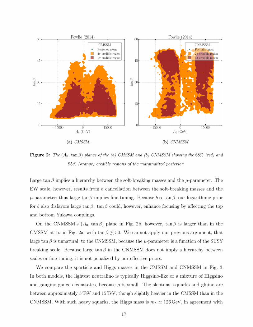
Figure 2: The (A0, tanβ) planes of the (a) CMSSM and (b) CNMSSM showing the 68% (red) and
95% (orange) credible regions of the marginalized posterior.
Large tan β implies a hierarchy between the soft-breaking masses and the µ-parameter. The
EW scale, however, results from a cancellation between the soft-breaking masses and the
µ-parameter; thus large tan β implies fine-tuning. Because b ∝ tan β, our logarithmic prior
for b also disfavors large tan β. tan β could, however, enhance focusing by affecting the top
and bottom Yukawa couplings.
On the CNMSSM’s (A0, tan β) plane in Fig. 2b, however, tan β is larger than in the
CMSSM at 1σ in Fig. 2a, with tan β . 50. We cannot apply our previous argument, that
large tan β is unnatural, to the CNMSSM, because the µ-parameter is a function of the SUSY
breaking scale. Because large tan β in the CNMSSM does not imply a hierarchy between
scales or fine-tuning, it is not penalized by our effective priors.
We compare the sparticle and Higgs masses in the CMSSM and CNMSSM in Fig. 3.
In both models, the lightest neutralino is typically Higgsino-like or a mixture of Higgsino
and gaugino gauge eigenstates, because µ is small. The sleptons, squarks and gluino are
between approximately 5TeV and 15TeV, though slightly heavier in the CMSSM than in the
CNMSSM. With such heavy squarks, the Higgs mass is mh ' 126GeV, in agreement with
17

χ01 χ
02 χ
03 χ
04 χ±1 χ±2 eL τ1 τ2 uL t1 t2 g H A H± h
Particle
0
5000
10000
15000
20000
25000
Mas
s(G
eV)
Fowlie (2014)
CMSSM2σ credible region
1σ credible region
Posterior mean
124.0
124.5
125.0
125.5
126.0
126.5
127.0
127.5
128.0
mh
(GeV
)(a) CMSSM.
χ01 χ
02 χ
03 χ
04 χ
05χ±1 χ±2 eL τ1 τ2 uL t1 t2 g h2 h3A1A2H± h
Particle
0
5000
10000
15000
20000
25000
Mas
s(G
eV)
Fowlie (2014)
CNMSSM2σ credible region
1σ credible region
Posterior mean
124.0
124.5
125.0
125.5
126.0
126.5
127.0
127.5
128.0
mh
(GeV
)
(b) CNMSSM.
Figure 3: Sparticle masses in the (a) CMSSM and (b) CNMSSM. The red and orange bars are the
68% and 95% credible regions for the sparticle masses. The green and blue bars are the 68% and
95% credible regions for the Higgs mass; note that the Higgs mass has a separate scale. The circles
are the posterior means.
experiment. In the CNMSSM, the Higgs with a mass of about 126GeV is always the lightest
Higgs. As anticipated, mh ' 126GeV is achieved in the CNMSSM with slightly lighter
sparticles than in the CMSSM, because of the CNMSSM’s additional tree-level contribution
to the Higgs mass in Eq. (4).
We further examine the Higgs mass in Fig. 4, in which we plot the one-dimensional PDF
for the Higgs mass in the CMSSM and in the CNMSSM. The PDF in the CMSSM and
CNMSSM are nearly identical.6 Whilst Eq. (4) indicates that the Higgs mass in the CNMSSM
ought to be heavier than that in the CMSSM, the similarity in the PDFs is unsurprising.
Our likelihood included a requirement that mh ∼ 126GeV.
Let us instead examine whether the additional tree-level contribution to the Higgs mass
in the CNMSSM in Eq. (4),
∆mh = λv sin 2β, (31)
is appreciable. This contribution is added in quadrature, m2h + ∆m2
h, weakening its impact.
We plot ∆mh and the relevant parameters, tan β and λ, in Fig. 5. The additional tree-level6 Minor differences in the PDF could result from statistical noise.
18

124.5 126.0 127.5 129.0mh (GeV)
0.00
0.25
0.50
0.75
1.00
Fowlie (2014)
CMSSMPosterior mean
Posterior PDF
2σ credible region
1σ credible region
(a) CMSSM.
124.5 126.0 127.5 129.0mh (GeV)
0.00
0.25
0.50
0.75
1.00
Fowlie (2014)
CNMSSMPosterior mean
Posterior PDF
2σ credible region
1σ credible region
(b) CNMSSM.
Figure 4: The predicted Higgs mass in the (a) CMSSM and (b) CNMSSM. The orange line is the
marginalized posterior PDF. The green and blue bars are the 68% and 95% credible regions for the
Higgs mass. The circles are the posterior means. So that the PDFs can be fairly compared, both
PDFs are normalized such that their integrals are identical.
contribution in the CNMSSM in Fig. 5a is negligible; with one tail at 1σ, ∆mh . 0.25GeV.
The smallness of this contribution stems from the smallness of λ in Fig. 5b; λ . 0.1 is favored,
although λ as large as 4π is permitted.
The smallness of λ was remarked upon in previous Bayesian studies of the CNMSSM [24,
50, 51], in which it was posited that small λ minimized the occurrence of tachyonic Higgs
bosons. Furthermore, Ref. [24] suggests that for mh ∼ 126GeV and tan β & 10, naturalness
priors might favor small λ (see e.g., Fig. 3 in Ref. [24]).
Ref. [19] remarks that if Aλ is large, increases in λ might decrease the Higgs mass. Because
we always select mh ∼ 126GeV, this behavior is difficult to study; however, Fig. 5c, a scatter
plot on the (λ,mh) plane, indicates that this behavior occurs. The highest Higgs mass
achieved decreases as λ is increased. We caution the reader that the scatter plot is misleading,
however, because the density of points cannot be resolved. There are many more points, and
19

0.0 0.6 1.2 1.8 2.4 3.0∆mh (GeV)
0.00
0.25
0.50
0.75
1.00
Fowlie (2014)
CNMSSMPosterior mean
Posterior PDF
2σ credible region
1σ credible region
(a) Additional tree-level contribution
to Higgs mass.
0.00 0.04 0.08 0.12 0.16 0.20λ
0
15
30
45
60
tanβ
Fowlie (2014)
CNMSSMPosterior mean
2σ credible region
1σ credible region
(b) (λ, tanβ) plane.
0.0 0.1 0.2 0.3 0.4 0.5λ
90
100
110
120
130
mh
(GeV
)
Fowlie (2014)
CNMSSMSamples with appreciable weight
(c) (λ,mh) plane.
Figure 5: (a) The additional tree-level contribution to Higgs mass in the CNMSSM. The orange
line is the marginalized posterior PDF. The green and blue bars are the 68% and 95% credible
regions. (b) The (λ, tanβ) plane in the CNMSSM showing the 68% (red) and 95% (orange) credible
regions of the marginalized posterior. (c) Samples with appreciable posterior weight scattered on the
(λ,mh) plane. The relationship between λ, tanβ and ∆mh is in Eq. (31).
much more posterior weight, with λ . 0.1. In fact, with one tail at 2σ, λ . 0.08.
With the Bayesian evidence, fine-tuning is a property of a “neighborhood” in a model’s
parameter space, i.e., the evidence in a “neighborhood” is a probability density multiplied
by a volume element. By itself, a probability density is not a well-defined property of an
individual point, because it is not e.g., invariant under reparameterizations. Ref. [85–87]
present individual points with small fine-tuning measures. We refrain from presenting such
points, because they have no particular probabilistic meaning.
B. Evidence
Let us recapitulate our aim. We wanted to find the Bayes-factor for the CNMSSM versus
the CMSSM. The Bayes-factor measures how our relative belief in the CNMSSM versus the
CMSSM ought to change in light of the experimental data. Bayesian naturalness of the EW
scale is automatically incorporated in the Bayes-factor. We interpret the Bayes-factor with
the Jeffreys’ scale in Table I.
20

If the Bayes-factor is greater than (less than) one, the CNMSSM (CMSSM) is favored.
The Bayes-factor was
B (CNMSSM/CMSSM) = 10+100−5 . (32)
The large uncertainty results from the evidence calculation in the CNMSSM.With a reasonable
computer time, (Py)MultiNest-3.4 found the CNMSSM’s evidence with an upper bound
one order of magnitude greater than its estimate and the CMSSM’s evidence to within a
factor of one half. These uncertainties could be reduced with extensive computing resources.
Fortunately, the uncertainty in the Bayes-factor corresponds to an uncertainty of a single
grade on the Jeffreys’ scale in Table I. The Bayes-factor is “positive” or “strong” evidence
in favor of the CNMSSM versus the CMSSM. “Positive” evidence is two grades below “very
strong” evidence and one grade above “barely worth mentioning.”
A factor of about 5 in this ratio, however, resulted from the difference in the prior volume
of µ in the CMSSM and κ in the CNMSSM in Table III;
ln(MP
1GeV
)ln(
4π0.001
) ≈ 5. (33)
This factor is related to the µ-problem (see e.g., [39]). Without this factor, the evidence in
favor of the CNMSSM versus the CMSSM is “barely worth mentioning” or “positive.” The
naturalness of the CNMSSM is overstated in the literature. The difference in the credibility
of the CNMSSM and CMSSM is “barely worth mentioning” or “positive,” unless one considers
the µ-problem. If one ignores the µ-problem, the evidence in favor of the CNMSSM is unlikely
to be “strong” and is certainly not “very strong.”
We anticipated that the CNMSSM would be more credible than the CMSSM, because
additional tree-level contributions to the Higgs mass in Eq. (4) might permit lighter stops.
Whilst the stops in the CNMSSM were slightly lighter than the stops in the CMSSM, the stops
were 3TeV . mt . 15TeV in each model (see Fig. 3). We found “barely worth mentioning”
to “positive” evidence that the agreement between generic predictions and experimental
data in the CNMSSM is better than that in the CMSSM, if one ignores the µ-problem, and
“positive” to “strong” evidence if one considers the µ-problem.
The final step, which we omit, is multiplying the Bayes-factor by one’s prior odds to find
one’s relative belief in the CNMSSM versus the CMSSM, in light of experimental data, i.e.,
the posterior odds in Eq. (13). When picking prior odds, one must discard knowledge of
the EW scale, all experimental data, the fact that the CNMSSM solves the µ-problem of
21

the CMSSM, and any other naturalness considerations that originate from knowledge of the
EW scale. To include such knowledge in one’s prior odds would be “double-counting;” it is
already included in the Bayes-factor.
Calculating Bayesian evidences is numerically challenging and we acknowledge that our
evidences suffered from substantial uncertainties. To help judge those uncertainties, we list
our MultiNest-3.4 settings in Table IV. We followed the recommendations in Ref. [88] for
an accurate calculation of the Bayesian evidence, with the exception of the stopping criteria
(the evidence tolerance) in the CNMSSM. Satisfying the stopping criteria recommended in
Ref. [88] in the CNMSSM would require extensive computing resources. As a consequence,
there is an appreciable uncertainty in the evidence in the CNMSSM, as already discussed.
CMSSM CNMSSM
Samples in posterior distribution 40 000 40 000
Total likelihood evaluations 400 000 1 100 000
Evidence tolerance 0.5 8
MultiNest v3.4 with gcc
Importance sampling True
Multimodal False
Constant efficiency False
Efficiency 1
Live points 4000
Table IV: Our settings for the MultiNest algorithm. For details, see the MultiNest
documentation [45].
C. Possible impact of DM
As mentioned in Sec. IVA, to avoid extra assumptions and sources of fine-tuning, we
omitted DM observables from our likelihood. One might wonder, however, how DM observ-
ables might impact our conclusions, were we to assume that the LSP accounted for all of the
DM in the Universe.
22

In the CNMSSM, because we find that in our results the singlino is decoupled, the singlino
is probably irrelevant to DM. We conjecture that DM observables could impact the posterior
PDF on the (m0, m1/2) plane in the CNMSSM and in the CMSSM. Common DM annihilation
mechanisms, such as coannihilation or resonances, preclude focusing of the EW scale, and
would be disfavored. Focus point regions in which the LSP is a fine-tuned bino-Higgsino
mixture could satisfy DM constraints [84]. Such regions would be favored.
It is unclear, however, how DM observables might impact the Bayes-factor, i.e., whether
DM might favor a particular model. Because the singlino is decoupled in the CNMSSM, in
each model, the most probable DM is a fine-tuned bino-Higgsino mixture. We find insufficient
reason to believe that such a fine-tuned mixture could be more readily achieved in a particular
model. As such, we conjecture that the inclusion of DM observables might not significantly
impact the Bayes-factor.
VI. CONCLUSIONS
We calculated the posterior PDF and evidence for the CNMSSM and the CMSSM with
naturalness priors, including relevant data from the LHC. Previous calculations of the
posterior PDF for the CNMSSM picked informative priors for (MZ , tan β) at the EW scale.
We picked “honest” priors for the model parameters in the Lagrangian and superpotential
at the GUT scale. Whilst such priors were calculated for the CNMSSM in Ref. [24], the
posterior PDF and evidence for the CNMSSM with such priors are absent in the literature.
We examined the credible regions of the CMSSM and CNMSSM, finding which regions of
parameter space were favored by Bayesian naturalness. Mechanisms that focus Higgs SUSY
breaking masses to the EW scale were favored. In each model, the SUSY breaking masses
were m1/2 . 8TeV and m0 . 15TeV, with squarks and sleptons ∼ 10TeV. The discovery
prospects at the LHC were limited; with 3000/fb of data, it is unlikely that the LHC could
discover either the CMSSM or the CNMSSM. Contrariwise, the HE-LHC would probably
discover the CMSSM or CNMSSM, were nature described by either model.
We computed the Bayes-factor for the CNMSSM versus the CMSSM. The calculation
involved moderate uncertainties that could be resolved with extensive computing resources.
We found that the evidence in favor of the CNMSSM versus the CMSSM is “positive” to
“strong” on the Jeffreys’ scale, but that if one ignores the µ-problem, the evidence is “barely
23

worth mentioning” to “positive.” “Positive” evidence is two grades below “very strong.” We
conclude that the credibility of the CNMSSM is perhaps overstated in the literature and that
the µ-problem must be considered in a comparison between the CNMSSM and CMSSM.
ACKNOWLEDGMENTS
This work was supported in part by grants IUT23-6, CERN+, and by the European Union
through the European Regional Development Fund and by ERDF project 3.2.0304.11-0313
Estonian Scientific Computing Infrastructure (ETAIS).
[1] E. Gildener, Phys.Rev. D14, 1667 (1976).
[2] L. Susskind, Phys.Rev. D20, 2619 (1979).
[3] A. Salam and J. Strathdee, Nucl.Phys. B76, 477 (1974).
[4] H. E. Haber and G. L. Kane, Phys.Rept. 117, 75 (1985).
[5] H. P. Nilles, Phys.Rept. 110, 1 (1984).
[6] S. P. Martin, (1997), arXiv:9709356 [hep-ph].
[7] H. Baer and X. Tata, Weak scale supersymmetry: From superfields to scattering events (Cam-
bridge University Press, 2006).
[8] M. Dine, Supersymmetry and string theory: Beyond the standard model (Cambridge University
Press, 2007).
[9] R. Barbieri and G. Giudice, Nucl.Phys. B306, 63 (1988).
[10] J. R. Ellis, K. Enqvist, D. V. Nanopoulos, and F. Zwirner, Mod.Phys.Lett. A1, 57 (1986).
[11] J. E. Kim and H. P. Nilles, Phys.Lett. B138, 150 (1984).
[12] P. Fayet, Nucl.Phys. B90, 104 (1975).
[13] J. Beringer et al. (Particle Data Group), Phys.Rev. D86, 010001 (2012).
[14] S. Chatrchyan et al. (CMS Collaboration), Phys.Lett. B716, 30 (2012), arXiv:1207.7235
[hep-ex].
[15] G. Aad et al. (ATLAS Collaboration), Phys.Lett. B716, 1 (2012), arXiv:1207.7214 [hep-ex].
[16] Search for squarks and gluinos with the ATLAS detector in final states with jets and missing
transverse momentum and 20.3 fb−1 of√s = 8 TeV proton-proton collision data, Tech. Rep.
24

ATLAS-CONF-2013-047, ATLAS-COM-CONF-2013-049 (CERN, 2013).
[17] S. Chatrchyan et al. (CMS Collaboration), JHEP 1406, 055 (2014), arXiv:1402.4770 [hep-ex].
[18] M. Maniatis, Int.J.Mod.Phys. A25, 3505 (2010), arXiv:0906.0777 [hep-ph].
[19] U. Ellwanger, C. Hugonie, and A. M. Teixeira, Phys.Rept. 496, 1 (2010), arXiv:0910.1785
[hep-ph].
[20] M. Bastero-Gil, C. Hugonie, S. King, D. Roy, and S. Vempati, Phys.Lett. B489, 359 (2000),
arXiv:hep-ph/0006198 [hep-ph].
[21] U. Ellwanger, G. Espitalier-Noel, and C. Hugonie, JHEP 1109, 105 (2011), arXiv:1107.2472
[hep-ph].
[22] M. Perelstein and B. Shakya, Phys.Rev. D88, 075003 (2013), arXiv:1208.0833 [hep-ph].
[23] S. King, M. Muhlleitner, R. Nevzorov, and K. Walz, Nucl.Phys. B870, 323 (2013),
arXiv:1211.5074 [hep-ph].
[24] D. Kim, P. Athron, C. Balázs, B. Farmer, and E. Hutchison, Phys. Rev. D 90, 055008 (2014).
[25] T. Gherghetta, B. von Harling, A. D. Medina, and M. A. Schmidt, JHEP 02, 032 (2013),
arXiv:1212.5243 [hep-ph].
[26] K. Agashe, Y. Cui, and R. Franceschini, JHEP 1302, 031 (2013), arXiv:1209.2115 [hep-ph].
[27] A. H. Chamseddine, R. L. Arnowitt, and P. Nath, Phys.Rev.Lett. 49, 970 (1982).
[28] R. L. Arnowitt and P. Nath, Phys.Rev.Lett. 69, 725 (1992).
[29] G. L. Kane, C. F. Kolda, L. Roszkowski, and J. D. Wells, Phys.Rev. D49, 6173 (1994),
arXiv:hep-ph/9312272 [hep-ph].
[30] J. Ellis and K. A. Olive, “Supersymmetric dark matter candidates,” in Particle Dark Matter:
Observations, Models and Searches, edited by G. Bertone (Cambridge University Press, 2010).
[31] U. Ellwanger, Phys.Lett. B133, 187 (1983).
[32] M. Carena, C. Grojean, M. Kado, and V. Sharma, “Status of Higgs physics,” in [13].
[33] C. Hugonie, G. Belanger, and A. Pukhov, JCAP 0711, 009 (2007), arXiv:0707.0628 [hep-ph].
[34] A. Djouadi, U. Ellwanger, and A. Teixeira, JHEP 0904, 031 (2009), arXiv:0811.2699 [hep-ph].
[35] N. Polonsky and A. Pomarol, Phys.Rev.Lett. 73, 2292 (1994), arXiv:hep-ph/9406224 [hep-ph].
[36] M. E. Cabrera, J. A. Casas, and R. Ruiz de Austri, JHEP 0903, 075 (2009), arXiv:0812.0536
[hep-ph].
[37] M. E. Cabrera, J. A. Casas, and R. Ruiz de Austri, JHEP 1005, 043 (2010), arXiv:0911.4686
[hep-ph].
25

[38] S. Fichet, Phys.Rev. D86, 125029 (2012), arXiv:1204.4940 [hep-ph].
[39] A. Fowlie, Phys.Rev. D90, 015010 (2014), arXiv:1403.3407 [hep-ph].
[40] H. Jeffreys, Theory of probability, 3rd ed. (Clarendon Press Oxford, 1961).
[41] R. E. Kass, Journal of the American Statistical Association 90, 773 (1995).
[42] A. Grinbaum, Foundations of Physics 42, 615 (2012), arXiv:0903.4055 [physics.hist-ph].
[43] D. J. C. MacKay, Bayesian Methods for Adaptive Models, Ph.D. thesis, California Institute of
Technology (1991).
[44] A. Fowlie and M. Raidal, Eur.Phys.J. C74, 2948 (2014), arXiv:1402.5419 [hep-ph].
[45] F. Feroz, M. Hobson, and M. Bridges, Mon.Not.Roy.Astron.Soc. 398, 1601 (2009),
arXiv:0809.3437 [astro-ph].
[46] J. Buchner, A. Georgakakis, K. Nandra, L. Hsu, C. Rangel, et al., Astron.Astrophys. 564, A125
(2014), arXiv:1402.0004 [astro-ph.HE].
[47] B. C. Allanach, Phys.Lett. B635, 123 (2006), arXiv:hep-ph/0601089 [hep-ph].
[48] B. C. Allanach, K. Cranmer, C. G. Lester, and A. M. Weber, JHEP 0708, 023 (2007),
arXiv:0705.0487 [hep-ph].
[49] M. E. Cabrera, J. A. Casas, and R. Ruiz de Austri, JHEP 1307, 182 (2013), arXiv:1212.4821
[hep-ph].
[50] D. E. Lopez-Fogliani, L. Roszkowski, R. Ruiz de Austri, and T. A. Varley, Phys.Rev. D80,
095013 (2009), arXiv:0906.4911 [hep-ph].
[51] K. Kowalska, S. Munir, L. Roszkowski, E. M. Sessolo, S. Trojanowski, and Y.-L. S. Tsai,
Phys.Rev. D87, 115010 (2013), arXiv:1211.1693 [hep-ph].
[52] B. C. Allanach, A. Djouadi, J. Kneur, W. Porod, and P. Slavich, JHEP 0409, 044 (2004),
arXiv:hep-ph/0406166 [hep-ph].
[53] P. Bechtle, S. Heinemeyer, O. Stål, T. Stefaniak, and G. Weiglein, Eur.Phys.J. C74, 2711
(2014), arXiv:1305.1933 [hep-ph].
[54] P. Bechtle, O. Brein, S. Heinemeyer, G. Weiglein, and K. E. Williams, Comput.Phys.Commun.
181, 138 (2010), arXiv:0811.4169 [hep-ph].
[55] P. Bechtle, O. Brein, S. Heinemeyer, G. Weiglein, and K. E. Williams, Comput.Phys.Commun.
182, 2605 (2011), arXiv:1102.1898 [hep-ph].
[56] P. Bechtle, O. Brein, S. Heinemeyer, O. Stål, T. Stefaniak, et al., PoS CHARGED2012, 024
(2012), arXiv:1301.2345 [hep-ph].
26

[57] P. Bechtle, O. Brein, S. Heinemeyer, O. Stål, T. Stefaniak, et al., Eur.Phys.J. C74, 2693 (2014),
arXiv:1311.0055 [hep-ph].
[58] B. C. Allanach, Phys.Rev. D83, 095019 (2011), arXiv:1102.3149 [hep-ph].
[59] P. Bechtle, B. Sarrazin, K. Desch, H. K. Dreiner, P. Wienemann, et al., Phys.Rev. D84, 011701
(2011), arXiv:1102.4693 [hep-ph].
[60] A. Fowlie, M. Kazana, K. Kowalska, S. Munir, L. Roszkowski, et al., Phys.Rev. D86, 075010
(2012), arXiv:1206.0264 [hep-ph].
[61] F. Mahmoudi, Comput.Phys.Commun. 178, 745 (2008), arXiv:0710.2067 [hep-ph].
[62] F. Mahmoudi, Comput.Phys.Commun. 180, 1579 (2009), arXiv:0808.3144 [hep-ph].
[63] F. Mahmoudi, Comput.Phys.Commun. 180, 1718 (2009).
[64] B. C. Allanach, Comput.Phys.Commun. 143, 305 (2002), arXiv:hep-ph/0104145 [hep-ph].
[65] B. Allanach, P. Athron, L. C. Tunstall, A. Voigt, and A. Williams, Comput.Phys.Commun.
185, 2322 (2014), arXiv:1311.7659 [hep-ph].
[66] S. Heinemeyer, W. Hollik, and G. Weiglein, Comput.Phys.Commun. 124, 76 (2000), arXiv:hep-
ph/9812320 [hep-ph].
[67] S. Heinemeyer, W. Hollik, and G. Weiglein, Eur.Phys.J. C9, 343 (1999), arXiv:hep-ph/9812472
[hep-ph].
[68] G. Degrassi, S. Heinemeyer, W. Hollik, P. Slavich, and G. Weiglein, Eur.Phys.J. C28, 133
(2003), arXiv:hep-ph/0212020 [hep-ph].
[69] M. Frank, T. Hahn, S. Heinemeyer, W. Hollik, H. Rzehak, et al., JHEP 0702, 047 (2007),
arXiv:hep-ph/0611326 [hep-ph].
[70] P. Ade et al. (Planck Collaboration), Astron.Astrophys. (2014), 10.1051/0004-6361/201321591,
arXiv:1303.5076 [astro-ph.CO].
[71] D. Akerib et al. (LUX Collaboration), Phys.Rev.Lett. 112, 091303 (2014), arXiv:1310.8214
[astro-ph.CO].
[72] H. Baer, V. Barger, and A. Mustafayev, JHEP 1205, 091 (2012), arXiv:1202.4038 [hep-ph].
[73] S. Heinemeyer, W. Hollik, and G. Weiglein, Phys.Rept. 425, 265 (2006), arXiv:hep-ph/0412214
[hep-ph].
[74] R. Ruiz de Austri, R. Trotta, and L. Roszkowski, JHEP 0605, 002 (2006), arXiv:hep-ph/0602028
[hep-ph].
[75] Y. Amhis et al. (Heavy Flavor Averaging Group), (2012), arXiv:1207.1158 [hep-ex].
27

[76] M. Misiak, H. Asatrian, K. Bieri, M. Czakon, A. Czarnecki, et al., Phys.Rev.Lett. 98, 022002
(2007), arXiv:hep-ph/0609232 [hep-ph].
[77] R. Trotta, F. Feroz, M. P. Hobson, L. Roszkowski, and R. Ruiz de Austri, JHEP 0812, 024
(2008), arXiv:0809.3792 [hep-ph].
[78] L. Roszkowski, E. M. Sessolo, and A. J. Williams, JHEP 1408, 067 (2014), arXiv:1405.4289
[hep-ph].
[79] K. Kowalska, L. Roszkowski, and E. M. Sessolo, JHEP 1306, 078 (2013), arXiv:1302.5956
[hep-ph].
[80] J. R. Ellis, T. Falk, and K. A. Olive, Phys.Lett. B444, 367 (1998), arXiv:hep-ph/9810360
[hep-ph].
[81] M. Drees and M. M. Nojiri, Phys.Rev. D47, 376 (1993), arXiv:hep-ph/9207234 [hep-ph].
[82] J. L. Feng, K. T. Matchev, and T. Moroi, Phys.Rev. D61, 075005 (2000), arXiv:hep-ph/9909334
[hep-ph].
[83] J. L. Feng and K. T. Matchev, Phys.Rev. D63, 095003 (2001), arXiv:hep-ph/0011356 [hep-ph].
[84] J. L. Feng, K. T. Matchev, and D. Sanford, Phys.Rev. D85, 075007 (2012), arXiv:1112.3021
[hep-ph].
[85] K. Kowalska, L. Roszkowski, E. M. Sessolo, and S. Trojanowski, JHEP 1404, 166 (2014),
arXiv:1402.1328 [hep-ph].
[86] A. Mustafayev and X. Tata, Indian J.Phys. 88, 991 (2014), arXiv:1404.1386 [hep-ph].
[87] H. Baer, V. Barger, D. Mickelson, and M. Padeffke-Kirkland, Phys.Rev. D89, 115019 (2014),
arXiv:1404.2277 [hep-ph].
[88] F. Feroz, K. Cranmer, M. Hobson, R. Ruiz de Austri, and R. Trotta, JHEP 1106, 042 (2011),
arXiv:1101.3296 [hep-ph].
28