SCANNING VOL. 35, 141–168 (2013)© Wiley Periodicals, Inc.

Is Scanning Electron Microscopy/Energy Dispersive X-raySpectrometry (SEM/EDS) Quantitative?

DALE E. NEWBURY* AND NICHOLAS W. M. RITCHIE

Surface and Microanalysis Science Division, National Institute of Standards and Technology, Gaithersburg,Maryland

Summary: Scanning electron microscopy/energy dis-persive X-ray spectrometry (SEM/EDS) is a widelyapplied elemental microanalysis method capable ofidentifying and quantifying all elements in the pe-riodic table except H, He, and Li. By following the“k-ratio” (unknown/standard) measurement proto-col development for electron-excited wavelength dis-persive spectrometry (WDS), SEM/EDS can achieveaccuracy and precision equivalent to WDS and atsubstantially lower electron dose, even when severeX-ray peak overlaps occur, provided sufficient countsare recorded. Achieving this level of performance isnow much more practical with the advent of the high-throughput silicon drift detector energy dispersive X-ray spectrometer (SDD-EDS). However, three mea-surement issues continue to diminish the impact ofSEM/EDS: (1) In the qualitative analysis (i.e., ele-ment identification) that must precede quantitativeanalysis, at least some current and many legacy soft-ware systems are vulnerable to occasional misidentifi-cation of major constituent peaks, with the frequencyof misidentifications rising significantly for minor andtrace constituents. (2) The use of standardless anal-ysis, which is subject to much broader systematic er-rors, leads to quantitative results that, while useful,do not have sufficient accuracy to solve critical prob-lems, e.g. determining the formula of a compound.(3) EDS spectrometers have such a large volume ofacceptance that apparently credible spectra can beobtained from specimens with complex topographythat introduce uncontrolled geometric factors thatmodify X-ray generation and propagation, resulting

†This article is a U.S. government work and, as such, is in the publicdomain in the United States of America.

*Address for reprints: Dale E. Newbury, Surface and Microanaly-sis Science Division, National Institute of Standards and Technology,Gaithersburg, MD 20899E-mail: dale.newbury@nist.gov

Received 10 May 2012; Accepted with revision 29 June 2012

DOI 10.1002/sca.21041Published online in Wiley Online Library (wileyonlinelibrary.com)

in very large systematic errors, often a factor of tenor more. SCANNING 00: 1–28, 2012. Published 2012Wiley Periodicals, Inc.†

Key words: elemental analysis, energy dispersiveX-ray spectrometry, EDS, scanning electronmicroscopy, SEM, silicon drift detector, SDD,quantitative analysis, X-ray microanalysis, X-rayspectrometry

Introduction

Scanning electron microscopy with energy disper-sive X-ray spectrometry (SEM/EDS) is an elemen-tal microanalysis technique widely applied across abroad range of the physical and biological sciences,engineering, technology, and forensic investigations(Goldstein et al., 2003). Electron-excited character-istic X-ray peaks provide identification and quantifi-cation for all elements of the periodic table, with theexceptions of H, He, and Li, that are present as majorconstituents (arbitrarily, a concentration C > 0.1 massfraction or 10 weight%), minor constituents (0.01 ≤C ≤ 0.1 mass fraction), and trace constituents (C <

0.01 mass fraction) to a limit of detection (CDL) typi-cally in the range 0.001–0.003 mass fraction depend-ing on the element of interest, the matrix in whichit resides, and the instrument operating conditions.With tens of thousands of SEMs equipped with EDSsystems operating worldwide, many thousands of ele-mental identifications and concentration determina-tions are reported daily. Qualitative and quantita-tive X-ray microanalysis techniques in the SEM haveevolved as a natural progression of the technique of“electron probe X-ray microanalysis (EPMA)” devel-oped by Castaing (’51). EPMA is a rigorous mea-surement method that follows strict requirements forspecimen preparation and for instrument operatingconditions, and EPMA quantitative analysis resultsare subject to a well-defined error budget that en-ables rigorous estimates of precision and accuracy

35: 141–168, 2013. †Published 2012Wiley Periodicals, Inc.

†This article is a U.S. government work and, as such, is in the public domain in the United States of America.

*Address for reprints: Dale E. Newbury, Surface and Microanaly-sis Science Division, National Institute of Standards and Technology, Gaithersburg, MD 20899E-mail: dale.newbury@nist.gov

Received 10 May 2012; Accepted with revision 29 June 2012

DOI 10.1002/sca.21041Published online 9 August 2012 in Wiley Online Library (wileyonlineli-brary.com)

142 SCANNING VOL. 35, 3 (2013)

(Goldstein et al., 2003). SEM/EDS is capable ofquantitative analysis with accuracy and precisionequivalent to wavelength dispersive spectrometry(WDS) analysis (Ritchie et al., 2012). However,SEM/EDS is often performed under much less con-trolled measurement conditions, especially with re-gard to the condition of the specimen and the locationof the beam on topographically complex surfaces. Areasonable question to ask is therefore: is SEM/EDSquantitative? This article will attempt to answer thisquestion with a review of the state of quantitative X-ray microanalysis as performed with SEM/EDS, be-ginning with a brief review of EPMA, which is widelyand justifiably regarded as the “gold standard” of el-emental microanalysis.

Development of Quantitative X-ray Microanalysis:Wavelength Dispersive X-ray Spectrometry

Quantitative electron-excited X-ray microanalysiswas first demonstrated by Castaing (’51) in the elec-tron probe X-ray microanalyzer (EPMA) that hedeveloped using WDS for X-ray intensity measure-ments. Castaing recognized that the efficiency of theWDS was a very complex function of photon energydue to the nature of the diffraction process, the needfor different diffraction crystals to cover the photonenergy range of analytical interest, and the variablesolid angle with photon energy, making the quanti-tative comparison of X-ray intensities between dif-ferent elements impractical due to the very largeuncertainties that resulted. To overcome this severelimitation, Castaing introduced a simple, elegantmeasurement solution: the “k-ratio” measurementprotocol in which the same X-ray peak was measuredfor the specimen (“spec”) and a standard (“std”) con-taining a known amount of that element under iden-tical instrumental conditions (generally in immediatesequence) to form a ratio of the X-ray intensities, Ix:

k = Ispec/Istd. (1)

Because the instrumental efficiency was identicalfor both measurements, this factor canceled quanti-tatively in the ratio. Castaing noted that this “k-ratio”was proportional to the ratio of mass concentrationsbetween the unknown and the standard. He devel-oped the physical basis for quantification by identify-ing a series of multiplicative “matrix correction fac-tors” applied to the k-ratio, which accounted for thecompositionally dependent effects of electron scatter-ing, electron energy loss (stopping power), primaryX-ray generation, X-ray absorption during propaga-tion through the material, and secondary X-ray gen-eration resulting from inner shell ionization by thephotoelectric absorption of the primary characteris-tic and bremsstrahlung (continuum) X-rays by atoms

of the sample. In its modern construction, the formulafor the calculation of relative concentrations has theform:

Cspec/Cstd = kZAF c, (2)

where Z is the “atomic number correction,” A is the“absorption correction,” and F and c are the “sec-ondary fluorescence corrections” for characteristic(F) and bremsstrahlung or continuum (c) radiation.As presented in Equation (2), Castaing’s approachseparates the instrumental measurement science ofthe k-ratio from the physical description of the gen-eration and propagation of X-rays embodied in thematrix corrections.

The WDS separates the X-ray photon energies onthe basis of Bragg diffraction from a crystal or artifi-cial layered material, a process that is sharply definedin angle. To maximize collected intensity, the WDSis constructed as a focusing device whose transmis-sion efficiency depends critically on precise position-ing of the X-ray source (the focused electron-beamimpact on the specimen), the diffracting crystal, andthe X-ray detector (gas ionization chamber). The fo-cusing properties of the WDS (mounted in the so-called “vertical geometry”) are so sharply defined atthe specimen that a few micrometers displacementof the specimen along the optic axis from the ideallevel causes a significant loss in measured intensity.Reproducible WDS measurement of X-ray intensi-ties requires precise specimen positioning, a conditionachieved in the EPMA by means of a fixed opticalmicroscope with an extremely shallow depth-of-focuspositioned to be in exact focus at the same positionas the WDS. Moreover, to satisfy the extremely lim-ited WDS focal volume as the specimen was movedlaterally, it was recognized that the specimen was re-quired to be optically flat. A flat surface was alsofound to be critical because Equation (2) implicitlyrequires that the only reason that the X-ray intensityfor an element differs between the specimen and thestandard is that the composition is different. Geomet-rical structures such as scratches with dimensions onthe micrometer scale similar to the electron interac-tion volume can significantly modify the generationand/or propagation of X-rays and introduce a largeand unpredictable error component (Yakowitz, ’68;Goldstein et al., 2003). WDS microanalysts quicklylearned that the only useful X-ray measurements werecareful measurements with a well-prepared, opticallypolished specimen/standard suite.

The accuracy achievable by WDS analysis fol-lowing the k-value measurement protocol with ma-trix corrections is illustrated by the relative errorhistogram in Figure 1 (Yakowitz, ’75). To constructthis histogram, materials of known composition(determined by independent bulk chemical analysis)that were demonstrated to be homogeneous on a

D. E. Newbury and N. W. M. Ritchie: Quantitative SEM/EDS analysis 143

Fig 1. Error distribution for quantitative X-ray microanalysiswith WDS k-ratio measurements and ZAF matrix corrections(NBS/NIST 1975 model; after Yakowitz, ’75).

micrometer scale (as determined with extensive sam-pling by electron-beam X-ray measurement) were an-alyzed with the method of Equation (2) using pureelements and simple compounds (e.g., FeS2 for S) asstandards. The k-ratios were measured to a high de-gree of precision (σ rel ≈ 0.5% or less) so that the ran-dom counting statistics portion of the error budgetis a small component of the distribution in Figure 1,which mostly depends on the systematic errors inher-ent in the particular matrix correction procedure ap-plied. All of the elements measured for Figure 1 werepresent as major constituents. The relative errors forFigure 1 were calculated as

Relative error = [(Measured − True)/True] × 100%.

(3)

By this definition, a positive relative error repre-sents overestimation of the true (reference) concen-tration while underestimating produces a negativerelative error. The error distribution in Figure 1 isapproximately symmetrical about zero relative errorand can be described as having a standard devia-tion of 2.5% relative error, so that approximately 95%of the analytical results fall within ±5% relative ofthe true value. Subsequent development of the ma-trix correction procedures by numerous workers overthe ensuing 50 years have further narrowed this errordistribution (e.g., Pouchou and Pichoir, ’91) so that

a reasonable estimate of current performance fromtheir work is that 95% of analyses should fall within±2.5% relative of the true value.

Development of Quantitative X-ray Microanalysis:Energy Dispersive X-ray Spectrometry with Si(Li)-EDS

The development by the radiation detectioncommunity in the 1960s of the semiconductorenergy dispersive X-ray spectrometer (EDS) basedon lithium-drifted silicon thick-crystal technology[Si(Li)-EDS] led to the first implementation of sucha device on an electron-beam column by Fitzgeraldet al., (’68). EDS provided an important advance overWDS because the entire excited X-ray spectrum froma threshold of ∼100 eV (current performance) tothe Duane–Hunt limit of the X-ray bremsstrahlungset by the incident electron-beam energy (maximumvalue typically 30 keV) was now recorded in everyEDS measurement. Having the complete X-ray spec-trum enabled a full qualitative analysis to identify theelements present at every analyzed location. The timepenalty for complete WDS scanning of the entirephoton energy range of interest is such that, evenwith modern highly automated computer-controlledWDS systems, it is not common practice to performa full qualitative analysis at every location sampledby the electron beam. EDS thus enabled a new levelof qualitative microanalysis whereby the analyst didnot risk failure in fully identifying major and minorconstituents that might be encountered unexpectedlywithin a heterogeneous material, a situation that fre-quently exists given the microstructural complexityof many unknowns.

Quantitative EDS analysis following the k-ratioprotocol was quickly demonstrated through the ef-forts of numerous researchers, including Reed andWare (’72), Schamber (’73), Lifshin et al. (’75),Fiori et al. (’76), and numerous others. Accurate ex-traction of characteristic peak intensities from thebresmsstrahlung background and from modest peakinterferences was demonstrated through tools suchas spectral filtering followed by multiple linear leastsquares (MLLS) fitting with experimentally measuredpeak references (Schamber, ’73). An example is givenin Table I (Newbury, 2000) of such an analysis of

TABLE I Analysis of NIST Standard Reference Material 482 (Cu–Au alloys) with Si(Li)-EDS and NIST-NIH DTSA (concentrationsin mass fraction)

Cu (SRM value) Analysis Rel error (%) Au (SRM value) Analysis Rel error (%) Raw analytical total

0.198 0.198 ± 0.0022 0.0 0.801 0.790 ± 0.0023 −1.4 0.9880.396 0.399 ± 0.0017 +0.8 0.603 0.594 ± 0.0027 −1.5 0.9930.599 0.605 ± 0.0014 +1.0 0.401 0.402 ± 0.0033 +0.2 1.0070.798 0.797 ± 0.0013 − 0.1 0.201 0.199 ± 0.0043 −1.0 0.996

1 − σ error in composition based upon net peak counts propagated through the matrix corrections; beam energy = 20 keV; CuKα

and AuLα; standards: pure Cu and Au (Newbury, 2000).

144 SCANNING VOL. 35, 3 (2013)

Fig 2. Comparison of k-ratios for Si, Ti, and Ba measured by WDS and SDD-EDS (Ritchie et al., 2012).

the National Institute of Standards and Technology(NIST) Cu–Au Alloy Standard Reference Material482 (Microanalysis Alloys) using Si(Li)-EDS spec-tra processed with the NIST-NIH Desktop Spec-trum Analyzer (DTSA) software (Fiori et al., ’92)with MLLS and the “NIST ZAF” atomic number-absorption-fluorescence matrix correction procedure(Myklebust et al., ’79). The relative errors for all eightconcentration determinations are less than 2% rela-tive, which fit well within the WDS relative error dis-tribution of Figure 1, and the analytical totals rangefrom 98.8% to 100.7%.

Recent Advances in Quantitative X-ray Microanalysis:Energy Dispersive X-ray Spectrometry with SDD-EDS

The emergence of the silicon drift detector en-ergy dispersive spectrometer (SDD-EDS) with its en-hanced peak stability and greatly improved through-put compared to Si(Li)-EDS has provided thebasis for an advance in analytical capability that chal-lenges one of the long standing assumptions aboutEDS compared to WDS (Struder et al., ’98; Newbury,

2005a). Because of its relatively poor spectral resolu-tion by a factor of ten or more, EDS has always beenconsidered to be inadequate for quantitative micro-analysis in critical situations when severe characteris-tic X-ray peak interference occurs. It has recently beendemonstrated that SDD-EDS with MLLS peak fit-ting can match WDS for intensity (k-ratio) measure-ments even when severe peak interference occurs formajor and minor constituents (Ritchie et al., 2012).High-count SDD-EDS spectra with five million ormore integrated spectral counts can be recorded inpractical measurement times of approximately 100 swith a conservative detector counting strategy (e.g., adead time of approximately 10%), which can serveas robust peak references for MLLS peak fitting.By comparison, Si(Li)-EDS spectra measured for thesame time at the same spectrometer resolution at 30%dead time contain approximately 100,000 counts. Ap-plying these statistically robust SDD-EDS peak ref-erences to MLLS peak fitting of similar high-countspectra of unknowns, X-ray peak intensities can beaccurately extracted from the X-ray continuum back-ground and from severely interfering peaks. An exam-ple is shown in Figure 2 for the interference of the Ba

D. E. Newbury and N. W. M. Ritchie: Quantitative SEM/EDS analysis 145

Fig 3. Extraction of k-ratios from spectra synthesized byadding experimentally measured pure element (Mo, Pb) andbinary compound (FeS2) spectra with DTSA-II spectrum mathtools followed by MLLS peak fitting with different experimen-tally measured spectra as peak references.

L3-M5 (Lα)–Ti K-L3 (Kα) peaks, which are separatedby 41 eV. A direct comparison was made of SDD-EDSand WDS k-ratios measured at the same locations forSi, Ti, and Ba on benitoite (BaTiSi3O9), barium ti-tanate (BaTiO3), and a series of Si–Ti–Ba glasses withvarious Ba/Ti ratios. The EDS spectra were processedwith the recently developed NIST DTSA-II softwareengine (Ritchie, 2011). The k-ratios measured withSDD-EDS and WDS are consistent within countingstatistics, even with a Ba/Ti mass fraction ratio above20:1.

These interference studies can be extended indi-rectly to other peak interference systems for whichsuitable microscopically homogeneous materials arenot available by using experimentally measured spec-tra of standards, which are then added in combina-tions using the spectrum calculator tools in DTSA-II.These summed spectra are then subjected to DTSA-II MLLS fitting using different standard spectra toserve as peak references. Examples of the results areshown in Figure 3 for the S K (2.307 keV), MoL2.293 keV, and PbM (2.346 keV). All three spectrawere combined, and then the S K intensity was de-creased successively to 0.5, 0.2, 0.1, 0.05, 0.02, and0.01 of the original level. The k-ratios recovered byMLLS fitting show excellent correspondence over thefull range, with only a 12% relative error in the k-ratiofor S K at a 100:1 reduction in intensity with inter-ference from both MoL and PbM. A similar studyis shown in Figure 4 for AgL-ThM, which not onlyfeatures a separation of only 12 eV (AgLα = 2.984keV; ThMα = 2.996 keV) for the principal peaks, butthe full AgL-family and ThM-family peak structuresoverlap over an extended energy range as seen in thesuperimposed spectra. The errors are somewhat larger

Fig 4. Extraction of k-ratios from Ag-Th spectra synthesizedby adding experimentally measured pure element spectra withDTSA-II spectrum math tools followed by MLLS peak fit-ting with different experimentally measured spectra as peakreferences.

in this extreme overlap case, reaching a 28% relativeerror in the k-ratio for an Ag/Th ratio of 100:1. Theseresults suggest that high-count SDD-EDS spectra canprovide access even with severe overlaps to the uppertrace concentration range (i.e., C > 0.001 mass frac-tion, 0.1 weight%).

The k-ratio measurement is the key step in achiev-ing quantitative X-ray microanalysis by EDS withequivalent performance, in terms of the error his-togram, to WDS. No matter which of the variousmatrix correction procedures is applied, accurate con-centration results depend upon starting with accuratek-ratio measurements. Thus, being able to duplicateWDS k-ratios on elemental mixtures with stronglyinterfering peaks means that the same level of quan-titative microanalysis accuracy available with WDScan now be achieved with SDD-EDS for major, mi-nor, and upper trace level constituents. Further workis currently underway to better define the lower levelof concentration that is practical with SDD-EDS, es-pecially when peak interference occurs. Of course, asthe concentration is lowered within the trace range,eventually a level will be reached where WDS is supe-rior to SDD-EDS because of its superior resolutionand its unique capability through the diffraction pro-cess of restricting the detector dead time to only thenarrow energy band of the photons of interest, ex-cluding dead time contributions from high-intensitypeaks of major constituent elements. However, for awide range of X-ray microanalysis problems involvingmajor, minor, and upper trace level constituents, care-fully following the k-ratio measurement protocol withSDD-EDS combined with control of the specimengeometry can provide robust, high confidence, andaccurate results.

146 SCANNING VOL. 35, 3 (2013)

Fig 5. Schematic illustration of the effect of local topographyon the X-ray path length to the detector. S = X-ray path lengthwithin specimen along detector axis; ψ = EDS detector takeoffangle, measured above the horizontal plane.

“Best Practices” EDS Quantitative X-RayMicroanalysis

To achieve optimum results, the analyst must beaware of his/her responsibilities to perform robustSEM/EDS measurement science. While a completelist of “best practices” for EDS quantitative X-raymicroanalysis must include specific procedures appro-priate to the particular SEM/EDS system in use, it isuseful to consider the most important general issues.

The Condition of the Specimen

Early in the history of the development of quantita-tive X-ray microanalysis, it was realized that a criticalissue affecting the error budget concerned the con-dition of the specimen surface. A “0th” assumptionof the model for quantitative X-ray microanalysis ex-pressed in Equation (2) is that the only reason the X-ray intensity measured for the unknown differs fromthe intensity measured for the standard is that thecomposition is different, and no other factor affectsthe X-ray intensity. “Geometric effects” are variationsin the local specimen topography that modify the elec-tron interactions such as backscattering, which affectstotal X-ray generation and the depth distribution. Asillustrated schematically in Figure 5, geometric ef-fects arising from local topographic structures suchas ridges and scratches, even fine-scale features withmicrometer dimensions similar to that of interactionvolume, can lead to strong changes in X-ray emis-sion, since photoelectric X-ray absorption follows anexponential law.

I/I0 = exp[−(μ/ρ)ρs], (4)

where I0 is the starting intensity, I is the intensityafter passage through a path s, (μ/ρ) is the mass

TABLE II Effect of surface condition on variability of measuredX-ray intensity

Surface AuMα σ AuLα σ

condition C.V. (%) (%) C.V. (%) (%)

600 grit SiC 8.6 0.13 1.8 0.31500 nm Al2O3 0.7 0.13 1.1 0.31100 nm Al2O3 0.46 0.13 0.42 0.31

Beam energy = 20 keV; 20 measurement locations; σ = singlepoint counting statistic = n1/2/n; C.V. = coefficient of variation= (σ distribution/mean) × 100%; data from Yakowitz (’68).

absorption coefficient for the particular composition,and ρ is the density. Low-energy photons below 4 keVin energy are especially susceptible to such absorptionpath length effects.

The issue of what constitutes a sufficiently flatspecimen to avoid geometric effects was consideredby Yakowitz (’68), who examined the impact of sur-face roughness on the variance in the measured X-ray intensity for various pure metals and alloys byinterrupting the metallographic grinding and polish-ing sequence after each step. Table II derived fromhis work shows the effects of specimen topographyon measured WDS X-ray intensity after three differ-ent polishing stages as observed on pure gold, whichprovides both high-energy (AuLα = 9.711 keV) andlow-energy (AuMα = 2.123 keV) characteristic X-raypeaks for simultaneous measurement. Comparison ofthe coefficient of variation for a suite of 20 fixed-beamlocation measurements with the single measurementcounting statistic showed that the specimen topog-raphy of the 600 grit (U.S. grading) surface signifi-cantly affected the measured intensity for both thehigh- and low-energy peaks, with the coefficient ofvariation greater by a factor of 6–60 than the relativestandard deviation of the peak count. For the 500-nmdiameter (nominal) alumina polish, the coefficient ofvariation was reduced to approximately three timesthe precision of the single measurement for the high-energy peak, while the 100-nm diameter (nominal)alumina polish was needed to achieve this correspon-dence for the low-energy peak. If even lower photonenergies are considered, especially below 1 keV, thensurface topography should be reduced further, to anamplitude below 20 nm, to minimize the influence oftopographic effects.

Operation of the EDS System

Before commencing any EDS microanalysis cam-paign, the analyst should follow an established check-list with careful attention to the measurement scienceof EDS operation:

D. E. Newbury and N. W. M. Ritchie: Quantitative SEM/EDS analysis 147

1. Choosing the EDS time constant (resolution): Be-fore the starting of any EDS measurement cam-paign, the choice of the EDS amplifier time con-stant (a generic term that may be locally knownas “shaping time,” “processing time,” “resolu-tion,” “count rate range,” “1–6,” etc.) should bechecked. There are usually at least two settings,one that optimizes resolution (at the cost of X-raythroughput) and one that optimizes throughput(at the cost of resolution). Confirming the desiredchoice of the time constant is absolutely criticalwhen the EDS system is in a multiuser environ-ment, since the previous user may have altered thisparameter.

2. Choosing the solid angle of the EDS: The solidangle � of a detector with an active area A ata distance r from the specimen is

� = A/r2. (5)

If the EDS is mounted on a movable arm that canalter the detector-to-specimen distance, then theuser must select a specific value for this distance forconsistency with archived standard spectra if theseare to be used in quantitative analysis procedures.Because of the exponent on the distance parameterr in Equation (5), a small error in r propagates to amuch larger error in the solid angle and thereforein the measured intensity.

3. Selecting a beam current that produces an accept-able level of system dead time: X-rays are generatedrandomly in time with an average rate determinedby the flux of electrons striking the specimen. TheEDS system can measure only one X-ray photon ata time so that it is effectively unavailable if anotherphoton arrives while the system is “busy” measur-ing the first photon, causing the second photon tobe excluded from measurement and effectively lost(depending on the progress in measuring the firstphoton when the second photon arrives, the firstphoton measurement may be excluded as well). Anautomatic correction function measures the timethat the detector is busy, and to compensate forpossible photon loss during this “dead time,” ad-ditional time is added at the conclusion of the user-specified time so that all measurements are madeon the basis of the same “live time” so as to achieveconstant dose. The level of activity of the EDS isreported to the user as a percentage “dead time,”which increases as the beam current increases. Thedead-time correction circuit can correct the mea-surement time over the full dead-time range to 60%or higher (Note that as a component of a qual-ity measurement system, the dead-time correctionfunction should be periodically checked by system-atically changing the beam current and compar-ing the measured X-ray intensity with predicted).However, as the dead time increases and the arrival

rate of X-rays at the EDS increases, “coincidenceevents” can occur when two X-rays enter the EDSspaced so closely in time that the pulse inspectionfunction will not recognize the two X-rays as dis-tinct events. Such coincidence creates a sum of thetwo photon energies, which results in an anoma-lous event incorrectly placed in the EDS spectrum(energy histogram). The coincidence event can in-volve any combination of characteristic and back-ground photons, but the distortion of the spec-trum that results from coincidence is most easilyobserved when two characteristic X-ray photonscombine to produce a “coincidence peak.” Thiseffect is illustrated in Figure 6 for a sequence ofspectra measured at increasing dead time showingthe ingrowth of a series of coincidence peaks asthe dead time increases. With the long pulses ofthe Si(Li) EDS technology, the pulse inspectionfunction was effective in minimizing coincidenceeffects to dead times in the range 20–30%. Withthe much shorter pulses of the SDD-EDS technol-ogy, the pulse inspection function is less effective,requiring dead times in the range of 10% to mini-mize coincidence peaks. Even with this restrictionon dead time, the SDD-EDS is still a factor often or more faster than Si(Li)-EDS for the sameresolution. In summary, as a critical step in estab-lishing a quality measurement strategy, the beamcurrent (for a specific EDS solid angle) should beselected to yield a dead time of approximately 25%[for SiLi)-EDS] or 10% [for SDD-EDS] on a targetwhere the excitation creates a high X-ray flux, suchas pure Al or Si. This beam current can then beused for all measurements with reasonable expec-tation that the dead time will be within acceptablelimits.

4. Performing the EDS energy calibration: If the en-ergy calibration is not correct, then the X-raypeaks will appear in the wrong locations, and allforms of peak identification can be expected tosuffer increased failures, and the subsequent peakintensity measurement may also be subject to in-creased error. The calibration procedure should beperformed according to the manufacturer’s speci-fications, the test spectrum (spectra) for this pro-cedure should be archived, and the dated recordof the calibration parameters stored as basic partof a best practices quality assurance plan. Sincecalibration usually makes use of two widely sepa-rated peaks, e.g. AlKα,β and CuKα, CuLα,β andCuKα, etc., the calibrated EDS should be checkedfor the peak accuracy for intermediate energies,e.g. TiKα and FeKα, as well as for peaks outsideof the calibration energy range: e.g. low photonenergy peaks such as C K and O K where non-linear behavior can occur, as well as high photonenergy peaks, e.g. PbLα.

148 SCANNING VOL. 35, 3 (2013)

Fig 6. (A) SDD-EDS spectrum of NIST SRM 470 (glass K412) at a throughput of 6.5 kHz and a dead time of 1% (logarithmicdisplay). (B) SDD-EDS spectra of SRM 470 (glass K412) over a wide range of throughput/dead time: from 6.5 kHz and 1% deadtime; to 1157 kHz and 66% dead time. Note the ingrowth of the coincidence peaks such as 2MgK, 2AlK, 2SiK, etc.

5. Recording adequate counts in the spectrum: Theconfidence of peak identification in qualitativeanalysis and the precision of quantitative EDS X-ray microanalysis benefit by increasing the numberof measured X-ray counts recorded in the spec-trum. What constitutes an adequate number ofX-ray counts depends on the particular analyt-ical task. For a precise peak intensity measure-ment, the analyst might seek to record sufficientcounts in a characteristic peak of interest abovethe local background so that the relative standarddeviation is lowered to a desired precision, e.g.σ rel = 1%, which corresponds to 10,000 countsabove background. To detect a peak, it is commonpractice to consider that the detectable level (limitof detection) is established when the characteristicintensity integrated over the channels that define

the peak exceeds three times the square root ofthe background intensity in those channels. Effec-tively, this is the background that would be mea-sured in a blank, which corresponds to a mate-rial composed of the same major/minor elementswithout the element of interest. In EDS micro-analysis practice a suitable blank is not usuallyavailable, so this background for the peak win-dow is usually estimated for the measured spec-trum either by background modeling constrainedby measurements of the background in nearby re-gions where no peaks are observed or by MLLSfitting of the peak region. The minimum level forquantitative analysis, the so-called determinationlimit, is defined as a level that exceeds the standarddeviation of the background by at least a factor often (Currie, ’68).

D. E. Newbury and N. W. M. Ritchie: Quantitative SEM/EDS analysis 149

The Software Tools

The modern SEM/EDS X-ray microanalysis sys-tem is typically implemented with a powerful, flexible,and extremely useful set of software tools to collect,interpret, and quantify X-ray spectra. These softwaretools have been developed by commercial vendorsthrough many years of effort by numerous scientistsand software engineers. Throughout its history, theEDS microanalysis instrumentation field has been atthe forefront of incorporating into the laboratory thelatest developments in computer hardware and soft-ware as well as employing algorithms based uponthe continually improving understanding of the un-derlying physical basis of electron-excited X-ray gen-eration, propagation, and detection. By making useof such commercial software tools for EDS spectralaccumulation and the NIST-NIH DTSA or NISTDTSA-II software engines for MLLS peak fittingwith matrix corrections for quantitative analysis, theexcellent analytical performance presented in TableI and Figures 2–4 was achieved by carefully follow-ing the EDS k-ratio protocol. Virtually all commer-cial software platforms allow similar implementationof the k-ratio/matrix correction protocol, meaningthat this level of analytical accuracy and precisionshould be available to all users of modern X-ray mi-croanalysis systems. However, it must be emphasizedthat the analyst must recognize his/her responsibil-ity to be a critical user of the software tools, under-standing the limits of the particular analytical sys-tem at hand and not acting as an unquestioning con-sumer of the apparent authority of a slickly formattedoutput.

Challenges to SEM/EDS Credibility

The Perception of Quantitative X-ray Microanalysiswith EDS

Despite the long history of SEM-EDS X-ray mi-croanalysis, EDS quantitative analysis has gener-ally been considered inferior to WDS quantitativeanalysis when highly reliable concentration resultsare needed. There appear to be at least three rea-sons for this state of affairs across the microanalysiscommunity:

1. reliance on automatic peak identification for qual-itative analysis and failure to recognize incorrectelemental assignments, which can occur even at themajor constituent level but which are a frequentproblem for minor and trace level constituents;

2. the domination of quantitative EDS microanalysisby standardless analysis procedures with broaderand often undefined error histograms; and

3. the use of SEM/EDS to measure X-ray spectraof specimens with uncontrolled geometry (size,shape, local inclination), which introduces unchar-acterized “geometric” errors with a magnitudemuch more significant than those noted above inthe discussion of the surface finish of an ideal spec-imen. Indeed, the errors introduced by extremespecimen geometry can be so large as to render thequantitative analysis results virtually meaningless.

4. If the promise of the extraordinary quantitativeX-ray microanalysis achievements demonstratedabove by high-count SDD-EDS are to be real-ized across the SEM microanalysis community, itis critical to understand these issues and developprocedures to address the problems.

Is SEM/EDS Qualitative?

Before quantitative analysis by SEM/EDS can beattempted, the critical first step of qualitative analysismust be considered. Qualitative SEM/EDS analysisis the assignment of elements to the characteristicX-ray peaks recognized in the EDS spectrum. Oftenconsidered to be a trivial problem, achieving robust,high-confidence qualitative EDS analysis is, in fact,a challenge even at the level of major constituents,but the level of difficulty increases greatly as the con-centration level decreases into the minor and tracelevels. Virtually all qualitative EDS analysis is per-formed with a software tool variously called “auto-matic peak identification,” “peak ID,” or a similarname. When invoked, automatic peak identificationapplies a mathematical algorithm to locate and mea-sure the photon energy of the characteristic peaksin the spectrum and then assigns elemental labelsfrom a database of elemental X-ray energy informa-tion. Given the longevity of SEM/EDS systems andthe on-going technical evolution of commercial au-tomatic peak identification products currently in use,users may encounter various types of peak locationstrategy and mathematical rigor. Other differences areencountered concerning the degree of incorporationof X-ray physics information such as the occurrenceof more than one X-ray family for an element or theextent to which minor X-ray family members within apeak series are considered. All of these factors bear onthe success of the peak identification. While a power-ful and useful tool, the automatic peak identificationsoftware should be considered to be only a startingsuggestion, which the careful, skeptical analyst willinspect manually to determine which elemental as-signments are valid. Obviously, a quantitative analysisbased upon a faulty assignment of elemental identi-ties is worthless. As with all software systems, thereare usually critical choices of parameters for whichthe user is responsible.

150 SCANNING VOL. 35, 3 (2013)

Choosing automatic peak identification softwareparameters

Before considering the performance of automaticpeak identification, several cautions must be raisedconcerning user-selectable parameters, which againcomprise “best practices” issues.

1. Peak threshold criterion: A user-selectable thresh-old criterion on the size of a peak relative tothe background counting statistics limits peaksto be considered for identification (alternatively,this parameter may be stated as a “minimum ac-ceptable concentration” for identification). Thethreshold criterion influences the concentrationlevel at which genuine peaks in the spectrum areconsidered in the final identification. Peaks cor-responding to trace or even minor constituentsmay be ignored depending on the threshold set-ting. The threshold parameter can also influencethe time during the spectral accumulation at whicha peak identification solution is first displayed.If the parameter is set too low, the peak detec-tion algorithm may trigger on statistical fluctu-ations in the background, creating false peaksand an apparent elemental identification solutionthat is not be stable. An example of this phe-nomenon is shown in Figure 7 for a sample ofiron, where the identifications of small “peaks”in the specimen (W, P, Pd, Ag, Ca, and La inFig. 7(A)) change markedly (Zn, As, Al, Au, andLa in Fig. 7(B)) with only a 10% change in the in-tegrated count. In fact, all of these apparent traceelements are manifestations of the statistical fluc-tuations in the continuum being misinterpreted aspeaks by the peak-finding algorithm, with the ex-ception of the La peak, common to both spec-tra, which is actually a misinterpretation of theFeKα Si-escape peak (6.400 − 1.740 = 4.66 keV;LaLα = 4.641keV). Unfortunately, some analystsmay be misled by the perceived authority of a soft-ware supplied solution, leading them to terminatethe spectral accumulation too early and thus to“freeze in” an incorrect peak identification solu-tion. It is thus important to be sure that sufficientcounts have been accumulated to achieve a stablepeak identification solution before proceeding toinspect the elemental results manually.

2. Editing the allowed elements: At least some com-mercial automatic peak identification systems al-low the user to delete certain elements from con-sideration in the final peak identification solu-tion because these elements are subject to frequentmisidentification with that particular software sys-tem. Some of these systems even set default lists of“forbidden elements” that the user must activelyact to defeat if these elements are to be consideredby the automatic peak identification tool. An ex-

Fig 7. (A) Si(Li)-EDS spectrum of iron showing apparenttrace element peaks marked by automatic peak identificationduring the spectrum accumulation. (B) Same spectrum afteronly 10% more counting time; note almost complete change inthe trace elements with the exception of La (actually the FeKα

escape peak).

ample of such a list embedded in a current softwarepackage is shown in Figure 8. Deleting elementsfrom consideration is an extremely bad idea sincethis action only serves to cover up failings in thepeak identification software, and this practice in-troduces the real hazard that if any of the “forbid-den” elements is actually present in the specimen itwill inevitably be ignored because it resides in theexclusion list.

3. Editing the allowed X-ray family members: Simi-larly, some automatic peak identification softwaresystems permit the user to disregard certain minorX-ray family members that occur with low relativeintensity, such as the (Ll (L3-M1), Lη (L2-M1), Mζ

(M4,5-N2,3), and M2-N4. Again, this exclusion ofinformation from consideration is likely to lead

D. E. Newbury and N. W. M. Ritchie: Quantitative SEM/EDS analysis 151

Fig 8. Example of a list of “forbidden” elements (element symbols grayed out) set as a default in a current software version.

to mistakes in peak identification. These low rel-ative intensity family members actually producedetectable peaks that are well separated in energyfrom those of the principal family members, espe-cially when the element in question is present as amajor constituent. The danger is that if these mi-nor family peaks are excluded from consideration,either from the database used for automatic iden-tification or from the “KLM” lines used to aidmanual qualitative analysis, then the unmarkedpeak(s) are likely to be assigned to an incorrectelement that will be interpreted as occurring at theminor or trace level.

Peak misidentificationThe careful analyst must be aware that even with

“best practices” EDS operation and optimum choicesmade for the parameters listed above, there remainsa significant possibility that peak misidentificationmay occur, even for major constituents that pro-duce the highest relative intensity peaks in the spec-trum and even with high counts (greatly in excessof 10,000 counts) in those peaks. Previous studieshave reported egregious peak misidentifications formajor constituents despite careful energy calibrationand high spectrum counts, such as BrLα,β misidenti-fied as AlKα,β, and PbMα,β misidentified as S Kα,β(Newbury 2005b). Table III lists some of the partic-ular element pairs or multiplets that have been ob-served to produce peak misidentifications even at thelevel of major constituents. (Note: this list may not becomplete). For older peak identification proceduresthat employed a peak-finding algorithm to locate asingle channel to represent a peak and a lookup ta-ble of peak channel energies to locate matching val-ues, it has been estimated that such egregious ele-mental misidentifications occur for approximately 3–5% of major constituent identifications when the en-tire periodic table (excluding H, He, and Li) must beconsidered. However this estimate is somewhat mis-

TABLE III Combinations of elements and characteristic peakfamilies likely to produce misidentifications

Photon energyrange (keV) Element (energy)

0.390–0.395 N K (0.392); ScL (0.395)0.510–0.525 O K (0.523); V L (0.511)0.670–0.710 F K (0.677); FeL (0.705)0.845–0.855 NeK (0.848); NiL (0.851)1.00–1.05 NaK (1.041); ZnL (1.012); PmM (1.032)1.20 to1.30 MgK (1.253); AsL (1.282); TbM (1.246)1.45–1.55 AlK (1.487); BrL (1.480); YbM (1.521)1.70 to1.80 SiK (1.740); RbL (1.694); SrL (1.806); TaM

(1.709); W M (1.774)1.90 to1.99 Y L (1.922); OsM (1.910)2.00–2.05 PK (2.013); ZrL (2.042); PtM (2.048)2.10–2.20 NbL (2.166); AuM (2.120); HgM (2.191)2.28–2.35 S K (2.307); MoL (2.293); PbM (2.342)2.40–2.45 TcL (2.424); BiM (2.419)2.60–2.70 ClK (2.621); RhL (2.696)2.95–3.00 ArK (2.956); AgL (2.983); ThM (2.996)3.10–3.20 CdL (3.132); U Mα (3.170)3.25–3.35 K Kα (3.312); InLα (3.285); U Mβ (3.336)4.45–4.55 TiKα (4.510); BaLα (4.467)

Note this is only a partial list; more problematic elementalcombinations are likely to be encountered.

leading, since the misidentification problem is nota random occurrence. For example, a system thatmisidentifies the BrL peak as AlK is highly likelyto make this mistake for all Br-containing speci-mens. More recently developed peak identificationsoftware procedures that use the entire peak shapewith MLLS fitting compared against library refer-ences and that also incorporate the physical rules forpeak occurrence (e.g., K–L and L–M relationshipsfor certain elements) have reduced the misidentifica-tion problem, but current work demonstrates that thisvery serious problem has not been eliminated fromall current automatic peak identification software.Examples of peak misidentification blunders for ma-jor constituents with a current software system are

152 SCANNING VOL. 35, 3 (2013)

TABLE IV EDS analysis of a high Tc superconductor crystal by standards-based k-ratio/ZAF and by two commercial standardlessquantitative analysis protocols (concentrations in mass fraction)

Method Y Rel Ba Rel Cu Rel Cu Formulaerr (%) err (%) err (%) peak

True 0.133 0.412 0.286 YBa2Cu3O7−xk-ratio/ZAF 0.138 +3.8 0.411 − 0.2 0.281 − 1.7 CuKα YBa2Cu3O6.8Standardless 1 0.173 +30 0.400 − 2.9 0.267 − 6.6 CuKα Y2Ba3Cu4O10Standardless 1 0.158 +19 0.362 − 12 0.316 +10.5 CuL Y2Ba3Cu6O12Standardless 2 0.165 +24 0.387 − 6.1 0.287 +0.35 CuKα Y2Ba3Cu5O11Standardless 2 0.168 +26 0.395 − 4.1 0.276 − 3.5 CuL Y4Ba6Cu9O21

k-ratio/ZAF: NIST-NIH Desktop Spectrum Analyzer with multiple linear least squares peak fitting; standards for k-ratio/ZAF:Y (element); Ba (NIST K309 glass); Cu (element); E0 = 20 keV.

Fig 9. (A) SDD-EDS spectrum of KBr showing misidentification of BrL as AlK. (B) SDD-EDS spectrum of NIST glass K240showing misidentification of ZrL as PtM.

presented in Figure 9, showing that some of theegregious problems observed in the 2005 study, e.g.AlK-BrL and ZrL-PtM, are still occurring. Someunexpected new problems are also observed, e.g. inFigure 10(A) the PbM- and L-family peaks are prop-

erly labeled in a sample of pure Pb, but in Figure 10(B)for a multielement glass containing a major lead con-stituent (C = 0.417 or 41.7 weight%) the PbM-familyis labeled with a combination of S K and TcL while theprominent PbL peaks are completely ignored. This is

D. E. Newbury and N. W. M. Ritchie: Quantitative SEM/EDS analysis 153

Fig 10. (A) SDD-EDS spectrum of high-purity Pb, showing correct labeling of the principal PbM and PbL peaks, but incorrectlabeling of PbM4,5-N2,3 (Mζ ) as W M and PbM2-N4 as CdL. (B) SDD-EDS spectrum of NIST glass K230 showing misidentificationof PbM as S K and TcL while ignoring the high-energy Pb L-family X-ray peaks.

a surprising observation, since the misadventures ofautomatic peak identification in any particular soft-ware system were found to be at least consistent inthe earlier studies (Newbury 2005b, 2007, 2009). Theinconsistency on pure lead and lead as a major con-stituent is therefore especially troubling. Note thatthe misidentification of Tc instead of Pb is especiallysuspicious since Tc is a highly radioactive artificiallysynthesized element (as is Pm), but remarkably thedefault list of “forbidden elements” for this partic-ular automatic peak identification software system,

illustrated in Figure 8, allows Tc while suppressingfrom consideration quite reasonable elements such asSr, Br, and Nb.

The frequency of misidentifications by all gener-ations of automatic peak identification software in-creases as the concentration of constituents dropsinto the minor and trace range (Newbury 2007,2009). The problem of correctly identifying traceconstituent peaks with high confidence and reli-ability is so difficult that some commercial sys-tems are actually internally constrained to avoid any

154 SCANNING VOL. 35, 3 (2013)

identification in the trace range by ignoring peakswith a low peak-to-background, leaving this diffi-cult and often critical characterization problem to theanalyst.

Best practice in qualitative X-ray microanalysisMajor constituents. The automatic peak identifica-tion software provides results that are a useful firststep, but the analyst must review each proposed ele-mental assignment. To avoid being misled by an egre-gious mistake from automatic peak identification ofa major constituent, the careful analyst will alwaysconfirm the suggested peak assignments by perform-ing manual peak identification using the availablecomputer-aided analysis tools (e.g., KLM markers,peak fitting tools, etc.). Such software tools for man-ual identification must be further augmented by theuser’s understanding of the basic physics of X-ray pro-duction, propagation, and detection, which may notbe incorporated in the automatic peak identificationsoftware. It is critical to know which characteristicpeaks are available for a particular element at a givenbeam energy (excitation energy) and which can be ac-cessed by modifying the beam energy within the limitsof the SEM. A good strategy to begin a qualitativeanalysis is to select an incident beam energy of 20keV, which will provide adequate excitation for peakswith photon energies as high as 12 keV. The confi-dence that can be assigned to a tentative elementalidentification increases greatly when more than oneX-ray peak or families of peaks can be identified. Forelements with atomic numbers below 15 (phospho-rus), only the Kα (K-L3) X-ray peak will be availablefor identification since the Kβ (K-M) for low-Z el-ements is either nonexistent, very low relative inten-sity, or not resolvable from Kα with EDS. Startingwith sulfur, and depending on the resolution perfor-mance of the EDS, additional family members willbe resolved, e.g. Kβ, and for higher Z elements, theL-shell and M-shell X-ray families become available.The presence of K-shell X-rays above 4 keV for anelement, e.g. TiKα, means that a corresponding L-shell X-ray is also excited and detectable. Similarly,L-shell X-rays above ∼4.5 keV, e.g. BaLα, means thatthe corresponding M-shell X-ray peaks are also avail-able. Studying the EDS spectra of pure elements andsimple binary compounds measured over a range ofbeam energies is extremely helpful for developing apractical understanding of this critical X-ray physics,which despite its value is not necessarily embedded inautomatic peak identification software as the exam-ples above demonstrate.

� With the practical knowledge gained from studyingX-ray spectra, the analyst can also develop strategyto choose the beam energy to deal with especially

difficult peak identification problems by ensuringadequate excitation for the peaks of interest, andpossibly by choosing a more appropriate beam en-ergy to optimize the measurement. Such strategyis especially important when complex specimenscontaining elements of low, intermediate and highatomic number are to be measured. A strategy ofrepeated measurements with two or more beam en-ergies may be required. For example, a higher beamenergy may be appropriate to excite an additionalX-ray families for elements of intermediate andhigh atomic number to increase the degree of con-fidence in the peak identification as noted above.However, an understanding of X-ray absorptionis important when dealing with low photon en-ergy peaks (E < 1 keV). Low-energy photons sufferhigher relative absorption compared with photonswith E > 1 keV, so that the depth of X-ray produc-tion in the target, which depends on the incidentbeam energy, can strongly influence the measuredrelative X-ray peak heights. Such high-absorptionsituations can be so severe as to lead to the ap-parent loss of even major constituents when theyare represented only by low-energy peaks. This sit-uation is illustrated for C in SiC measured withE0 = 20 keV in Figure 11(A). C in Si representsa high-absorption situation because the Si L-shellabsorption edges at ∼100 eV are located below theenergy of the C K characteristic X-ray at 282 eV.At E0 = 20 keV, the self-absorption of the C in SiCreduces its intensity relative to the Si peak so muchso that when the vertical display range is limitedby the height of the Si peak, the C K peak is notvisible as a distinct peak. The SiC specimen mightbe mistakenly interpreted as pure Si. Increasing theescape of C X-rays requires lowering the beam en-ergy, so that with E0 = 3 keV, the C K X-ray peakbecomes readily apparent in Figure 11(B) as a ma-jor constituent.

Minor/trace constituents. The most challengingpeak identification problem is that of achieving a ro-bust level of confidence in identifying minor (0.01 ≤C ≤ 0.1 mass fraction) and trace level (C < 0.01 massfraction) constituents. Minor/trace constituent iden-tification requires a careful, systematic approach thatemphasizes comprehensive spectral study. First, eachmajor constituent must be identified and all princi-pal and minor X-ray family members of that elementas well as all associated spectral artifacts (Si-escapepeaks, coincidence peaks) must be located before pro-ceeding to identify any remaining low relative inten-sity peaks as arising from minor constituents andeventually trace constituents. Examples of peak iden-tification mistakes at the minor/trace level observedwith current software products include

D. E. Newbury and N. W. M. Ritchie: Quantitative SEM/EDS analysis 155

Fig 11. (A) Si(Li)-EDS spectrum of SiC with a beam energyof 20 keV. (B) Si(Li)-EDS spectrum of SiC with a beam energyof 3 keV.

1. Identifying false low level peaks by misinterpret-ing random statistical variations in the X-raybremsstrahlung, as shown in Figure 7.

2. Failure to correctly assign minor X-ray familymembers of an identified major constituent is oftenfollowed by mislabeling those minor peaks as anincorrect element(s), as illustrated by the spectrumof pure Pb in Figure 10(A), where the PbM4,5-N2,3

(Mζ ) is mislabeled as W M and the PbM2-N4 asCdL.

3. Escape peaks and coincidence peaks are com-monly misinterpreted by automatic peak identi-fication systems because the rules governing theseartifacts may not be embedded in the software pro-cedures. Examples of misidentification of peak co-

incidence commonly encountered include the AlKcoincidence identified as trace Ag and SiK coinci-dence identified as trace Sn shown in Figure 12(A)and (B). The misidentification of the Si escape peakis illustrated in Figure 13 for CrKα (5.411 keV),where the escape peak at 3.674 keV is misidenti-fied as Ca K-L3 (Kα) (3.690 keV). Note also themisinterpretation of the Cr K-shell sum peaks asBiL and SeL in this same spectrum.

The degree of confidence that can be placed in anelemental assignment inevitably declines as the con-centration of a constituent decreases into the minorand trace ranges. The number of recognizable peaksavailable to make the identification is diminished be-cause of the reduced counts in the minor X-ray familymembers. Improving the confidence in minor/traceconstituent identification can only be achieved by in-vesting longer spectral accumulation times to greatlyincrease the X-ray counts for low relative intensitypeaks. With the new class of SDD-EDS detectors,large spectral integrals can be accumulated within ac-ceptable time periods, e.g. 500 s or less to make pos-sible more reliable minor/trace constituent analysis.However, the much faster pulses of the SDD-EDSlead to significant coincidence peak problems as il-lustrated in Figure 2. There is thus a conflict betweenthe desire for high integral spectrum counts, obtainingthose high counts as quickly as possible by exploit-ing the full throughput of SDD-EDS, and obtainingspectra with minimal artifacts. The SDD-EDS pulsecoincidence problem leads to such significant spec-tral artifacts that it is recommended that throughputbe restricted to dead time below 10% unless carefulstudy of spectra justifies higher throughput, e.g. coin-cidence may occur, but not in the region of the spec-trum where the true minor/trace constituent peaks ofinterest occur.

Standardless Quantitative Analysis

The second major issue affecting the status ofEDS as a reliable quantitative analysis method isthe widespread, indeed dominant, use of “standard-less” quantitative analysis procedures. Probably 95%or more of the concentration results reported bySEM/EDS analysts are now derived from commer-cial “standardless” analysis software. The “standard-less” protocol is an extremely attractive “one-button”procedure for use in the SEM/EDS measurementenvironment that apparently requires little interven-tion by the analyst. The EDS spectrum provides si-multaneous (in energy, not time) measurement ofthe entire X-ray spectrum as excited in the SEM,in principle capturing all of the information neededfor comprehensive compositional analysis in a single

156 SCANNING VOL. 35, 3 (2013)

Fig 12. (A) SDD-EDS spectrum of Al with a beam energy of 20 keV showing misidentification of the Al coincidence peak as AgL.(B) SDD-EDS spectrum of Si with a beam energy of 20 keV showing misidentification of the Si coincidence peak as SnL.

measurement. The standardless analysis protocolonly requires the list of elements to be analyzed, whichis typically and often automatically supplied by thepeak identification software, the incident beam en-ergy and the emergence angle of the X-rays above thesurface (the so-called X-ray “takeoff” angle). Basedupon libraries of stored information, the relative X-ray intensities of the various elemental peaks are con-verted into relative concentrations and these valuesare scaled to unity (100 weight%), often with oxy-gen calculated indirectly by the method of assumedstoichiometry of the cations rather than measureddirectly. Scaling to unity is needed to put the finalvalues on a sensible basis, a direct requirement be-cause of the loss of electron dose information cor-related between the actual measurement conditionsand the reference database. Thus, the analytical total

in standardless procedures must inevitably total unity,even if a major constituent is inadvertently lost fromthe qualitative analysis. Two distinct classes of “stan-dardless” analysis exist: (1) “first principles" and (2)“remote standards.” Newbury et al. (’95) examinedboth classes of standardless analysis in a study thatinvolved quantitatively analyzing a suite of knownmaterials, including NIST Standard Reference Ma-terials, Research Materials, binary compounds, andhomogeneous alloys and glasses, to develop error his-tograms for standardless analysis similar to that ofFigure 1 for the WDS k-ratio protocol and ZAF ma-trix corrections. In that study, only X-ray peaks withphoton energies above 0.93 keV (CuL) were consid-ered, all constituents were present at major or highminor concentrations, and oxygen when present wastreated by the method of assumed stoichiometry.

D. E. Newbury and N. W. M. Ritchie: Quantitative SEM/EDS analysis 157

Fig 13. SDD-EDS spectrum of Cr with a beam energy of 20 keV showing misidentification of the Si-escape peak of CrK as CaKand the Cr coincidence peaks as BiL and SeK.

“First principles” standardless analysis“First principles” standardless analysis uses phys-

ical descriptions of the generation, propagation, anddetection of X-rays along with databases of physicalconstants such as ionization cross sections, the depthdistribution of ionization, fluorescence yields, massabsorption coefficients, the structure and thicknessdimensions of the X-ray detector, etc., to effectivelycompare intensities of X-ray peaks measured at dif-ferent photon energies. The accuracy of this methoddepends greatly on the availability and reliability ofmany physical constants as well as having an accuratemodel of the detection efficiency as a function of pho-ton energy, since the efficiency no longer cancels as itdoes in the k-ratio protocol described above. The firstprinciples model (Standardless Miracle) embedded inNIST-NIH Desktop Spectrum Analyzer was exam-ined in the 1995 study and the error histogram shownin Figure 14 was obtained (Newbury et al., ’95). Thiserror histogram is roughly symmetrical about zerorelative error, but the error bins are 10% relative wide,a factor of ten greater than the scale of the error his-togram of Figure 1 for the k-ratio protocol with ZAFmatrix corrections. The standard deviation of the firstprinciples standardless error histogram is such thatthe error range spans ±50% relative to capture 95%of the analyses. This broad error range is most likelycaused by uncertainties in many of the models andthe necessary parameters for X-ray generation, andlimitations in modeling the detector efficiency as afunction of photon energy. In the k-ratio protocolwhere each characteristic X-ray peak measured forthe unknown is compared with the same X-ray peakfrom a standard, accurate knowledge of the physicalbasis of X-ray generation is much less important than

Fig 14. Relative error histogram for a “first principles” stan-dardless analysis protocol (“Standardless Mircacle” in NIST-NIH Desktop Spectrum Analyzer; Newbury et al., ’95).

it is for standardless analysis where different X-raypeaks must be directly compared.

“Remote standards” standardless analysisMost commercial software implementations of

standardless analysis probably follow the “remotestandards” protocol (“probably” is used here becausethese methods are usually “black box” software pro-vided to the user without detailed documentation).Strictly speaking, the “remote standards” protocol isnot a true standardless procedure but a method totransfer a carefully measured library suite of stan-dard intensities to the local SEM/EDS measure-ment environment. The suite of known standards, e.g.pure elements and stoichiometric binary compounds

158 SCANNING VOL. 35, 3 (2013)

Fig 15. Relative error histogram for a commercial standard-less analysis protocol (Newbury et al., ’95).

(which are converted by appropriate matrix elementcalculations into equivalent pure element intensi-ties), is measured at several beam energies and at aconsistent dose (beam current × live time) with awell-characterized EDS for which the efficiency as afunction of photon energy is known. The resultingdatabase of remotely measured elemental intensitiesmust be adjusted to the local EDS photon efficiencyfor the particular peak(s) of interest through a detec-tor efficiency transfer calculation usually constrainedby a comparison of the X-ray continuum measuredon a “pure” continuum spectrum such as that fromhigh-purity carbon, which is minimally affected bythe C K characteristic peak. If the local measurementis made with a beam energy different from those rep-resented in the database, then the database standardintensity is adjusted using a model for the energydependence of X-ray generation constrained by theknown values in the database. Similarly, if the stan-dard intensity is required for an element not repre-sented in the database, then the needed value is againestimated with a physical equation for X-ray genera-tion constrained by the measured values for elementswith similar atomic numbers. Because the local doseis not taken into account in this method, the analyti-cal total must again be normalized to unity. Figure 15presents a relative error histogram for a commercialsoftware implementation of “standardless” analysisthat was acknowledged by the vendor to follow theremote standards protocol. Again the relative errorhistogram is approximately symmetrical, but the er-ror bins are a factor of five wider than the error binsin Figure 1. The standard deviation for this remotestandards standardless error histogram is such thatthe error range spans ±25% relative to capture 95%of the analyses.

There is nothing wrong with utilizing a standard-less analysis protocol providing the eventual user of

the analytical results understands the full implica-tions of the contribution to the measurement uncer-tainty budget that arises from whatever quantitativeanalysis protocol is used. However, the error contri-bution of the quantitative analysis procedure is oftennot mentioned to the final user of the data becausethe analyst may be unaware of its magnitude. Com-mercial standardless analysis software may be sup-plied without this important information (a carefulpurchaser would be very wise to ask for this infor-mation from a prospective vendor). Instead, the onlyexplicit contribution to the uncertainty budget thatis consistently reported is the measurement precisionfor each element, which is related to the number ofX-ray counts accumulated in the characteristic peakof interest and is readily calculable. With reasonablepatience by the analyst, the single measurement pre-cision can often be reduced to 0.5% relative or less(i.e., 40,000 counts in the integrated peak above back-ground), in a measurement time of 100 s, especiallywith the high-throughput SDD-EDS. While achiev-ing excellent measurement precision is important foroptimizing the performance of spectral fitting proce-dures and for comparing measurements at differentlocations in the specimen, the overall uncertainty bud-get for the measurement is dominated by the muchlarger contribution from the quantification method,even in the case of the EDS k-ratio/ZAF protocol.Considering the error distribution for “remote stan-dards” standardless analysis in Figure 15, what is theconsequence of relative errors in the range ±25%on the utility of final results? Consider that the an-alyst’s problem is to determine the formula of a com-pound. Table IV gives the results of the analysis ofa YBa2Cu3O7−x single crystal as performed with theEDS k-value/ZAF matrix corrections protocol andwith two different commercial standardless analysisprocedures, all with oxygen calculated by means ofassumed stoichiometry. For the standardless proce-dures, analysis with CuKα peak as well as with CuLpeak was tested. The errors for the three elements werewithin ±4% relative for the EDS k-value/ZAF proto-col, which results in the integer formula YBa2Cu3O6.8

that closely matches the result from independent neu-tron scattering crystallography measurements. Whilesome of the errors for Ba and Cu with standardlessanalysis protocols are less than 5% relative, the errorfor Y is consistently large, with the result that the for-mulae deduced from the standardless EDS analysisdiffer significantly from the correct value.

Standardless analysis, both the first principles andremote standards methods, is a subject of inten-sive continuing research (e.g., Duncumb et al., 2001;Statham 2002, 2006) and there has undoubtedly beenmuch progress since the 1995 study described above.It can be hoped that eventually standardless pro-cedures will match the performance of the EDS

D. E. Newbury and N. W. M. Ritchie: Quantitative SEM/EDS analysis 159

TABLE V Standardless analysis of sulfide minerals with a current commercial standardless analysis protocol (concentrations inmass fraction)

DerivedMineral Metal Rel err (%) S Rel err (%) formula

Troilite (FeS) 0.629 −1.1 0.371 +1.8 FeSCovellite (CuS) 0.764 +15 0.236 −30 Cu3S2Sphalerite (ZnS) 0.762 +14 0.239 −28 Zn3S2

k-value/matrix corrections protocol. However, theanalyst should not assume that the standardlessprocedure available in even the latest commercialsoftware is free from the significant errors seen inFigure 15. Table V gives results from a current(2011), recently updated version of a commercialstandardless analysis protocol applied to the anal-ysis of metal sulfide minerals. These materials werecomounted in the same block and the SDD-EDSspectra were recorded in succession so the perfor-mance of the spectrometer was identical during themeasurement sequence. The analysis of the mete-oritic mineral troilite resulted in sufficiently smallerrors that the correct formula, FeS, could be de-duced from the concentrations. However, the analysisof the minerals covellite (CuS) and sphalerite (ZnS)resulted in such large relative errors that incorrectformulae result. These analytical results are part ofan on-going comprehensive study updating the 1995evaluation by testing current standardless analysissoftware.

Uncontrolled Specimen Geometry

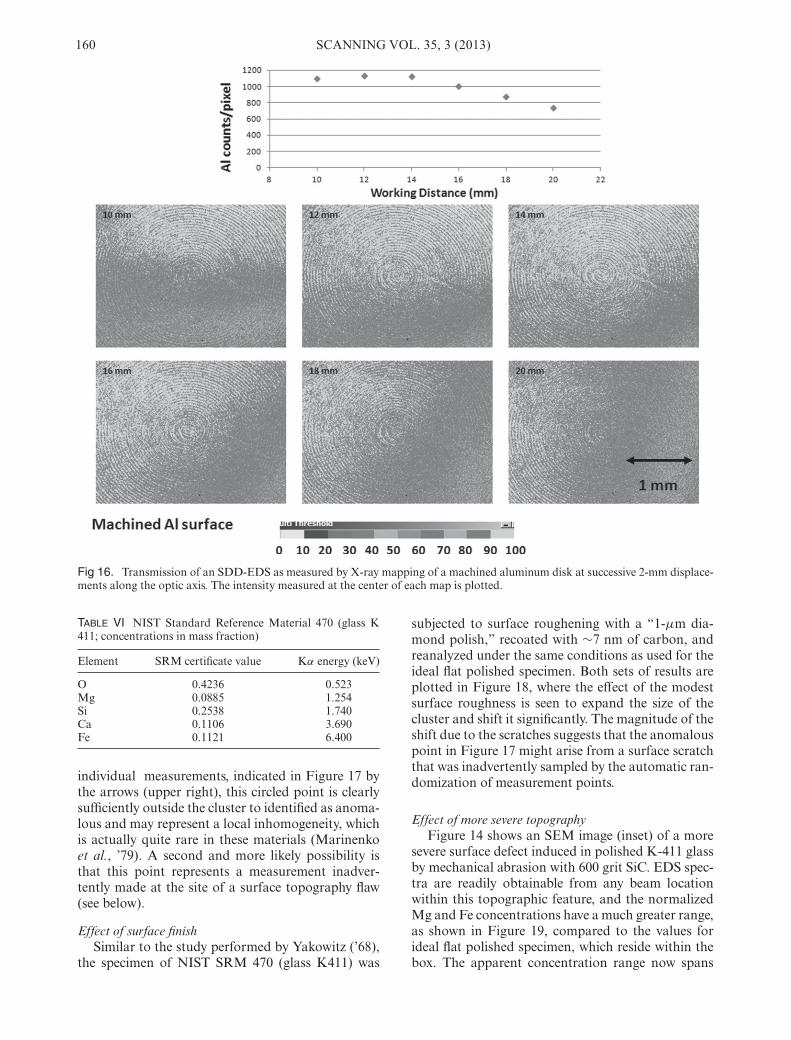
The third component that leads to questionableEDS analysis, and probably the factor with the high-est practical impact on the credibility of quantitativeSEM/EDS, is the lack of control of the specimen ge-ometry. As described above, the focusing properties ofWDS are so sharply defined that precise positioningof a very flat specimen is necessary for useful, repro-ducible X-ray intensities to be measured. Deviationsfrom the ideal focus location of only a few microm-eters along the optic axis and tens of micrometerslaterally cause significant decreases in X-ray inten-sities. The nonfocusing EDS is not subject to suchconstraints. Even with a properly mounted collima-tor, the EDS acceptance volume at the specimen hasdimensions of millimeters along all three axes. Thevolume of transmission for a particular SDD-EDS isshown in Figure 16, where a series of Al X-ray mapstaken at positions spaced by 2 mm along the opticaxis (for a detector optimized for a 10-mm workingdistance) are shown, along with a plot of the intensityat the center of each map. Over a total displacementof 1 cm, the center intensity varies by less than 30%,

and the lateral variation is generally less than 25%over a displacement of 2 mm. Such a large accep-tance volume means that EDS X-ray spectra can beobtained from rough, topographic objects at beamlocations where the generation of X-rays is substan-tially affected by the local specimen topography dueto modification of electron penetration and backscat-tering effects caused by the local thickness and theinclination to the beam. Specimen topography canhave even greater impact on the measured X-ray spec-trum. The target shape and dimensions can modifythe local X-ray absorption path to the detector sothat it deviates significantly from the ideal absorptionpath assumed in the quantification models appropri-ate to a flat specimen placed at carefully controlledelectron-beam incidence and X-ray takeoff angles.The collective result of these complex “geometric ef-fects” is to modify the measured X-ray intensities, of-ten quite substantially, from what would be measuredfor the ideal flat specimen properly located. One ofthe basic assumptions of quantitative microanalysisprocedures, for both standards-based and standard-less procedures alike, is that only composition affectsthe X-ray intensities. When this condition is violated,very large errors, far exceeding what is expected froman error histogram such as Figure 1 or Figure 15, canoccur.

To demonstrate the impact of such geometric fac-tors, a series of tests has been performed on NISTSRM 470 (K411 glass), the composition of whichis given in Table VI. K411 provides a range of X-ray energies from the energetic FeKα peak at 6.400keV, which is relatively unabsorbed to the low-energyMgKα peak at 1.254 keV, which is sensitive to ab-sorption effects. The dispersion of results from analy-sis with the NIST DTSA-II software engine of K411in the form of an ideal flat polished specimen isshown in Figure 17. A beam energy of 20 keV wasused, and the standards were Mg (element), Si (ele-ment), Ca (SRM glass K-412), and Fe (element), andthe results were normalized for direct comparison inthe following studies. The mean of the 20 measure-ments lies within +1.8% relative of the SRM valuefor Fe and −1.0% relative of the SRM value for Mg.Both the Fe and Mg results cluster within a rangeof approximately 1% relative, with one exception (cir-cled). Considering the concentration precision of the

160 SCANNING VOL. 35, 3 (2013)

Fig 16. Transmission of an SDD-EDS as measured by X-ray mapping of a machined aluminum disk at successive 2-mm displace-ments along the optic axis. The intensity measured at the center of each map is plotted.

TABLE VI NIST Standard Reference Material 470 (glass K411; concentrations in mass fraction)

Element SRM certificate value Kα energy (keV)

O 0.4236 0.523Mg 0.0885 1.254Si 0.2538 1.740Ca 0.1106 3.690Fe 0.1121 6.400

individual measurements, indicated in Figure 17 bythe arrows (upper right), this circled point is clearlysufficiently outside the cluster to identified as anoma-lous and may represent a local inhomogeneity, whichis actually quite rare in these materials (Marinenkoet al., ’79). A second and more likely possibility isthat this point represents a measurement inadver-tently made at the site of a surface topography flaw(see below).

Effect of surface finishSimilar to the study performed by Yakowitz (’68),

the specimen of NIST SRM 470 (glass K411) was

subjected to surface roughening with a “1-μm dia-mond polish,” recoated with ∼7 nm of carbon, andreanalyzed under the same conditions as used for theideal flat polished specimen. Both sets of results areplotted in Figure 18, where the effect of the modestsurface roughness is seen to expand the size of thecluster and shift it significantly. The magnitude of theshift due to the scratches suggests that the anomalouspoint in Figure 17 might arise from a surface scratchthat was inadvertently sampled by the automatic ran-domization of measurement points.

Effect of more severe topographyFigure 14 shows an SEM image (inset) of a more

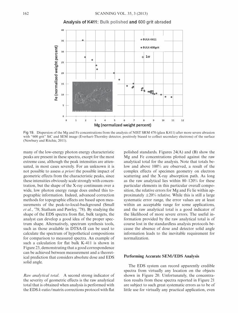
severe surface defect induced in polished K-411 glassby mechanical abrasion with 600 grit SiC. EDS spec-tra are readily obtainable from any beam locationwithin this topographic feature, and the normalizedMg and Fe concentrations have a much greater range,as shown in Figure 19, compared to the values forideal flat polished specimen, which reside within thebox. The apparent concentration range now spans

D. E. Newbury and N. W. M. Ritchie: Quantitative SEM/EDS analysis 161

Fig 17. Dispersion of the Mg and Fe concentrations from the analysis of NIST SRM 470 (glass K411) in the ideal flat, polishedform. Beam energy = 20 keV. 1 − σ counting statistics expressed as a concentration uncertainty are shown. Note outlier point(circled; Newbury and Ritchie, 2011).

Fig 18. Dispersion of the Mg and Fe concentrations from the analysis of NIST SRM 470 (glass K411) after abrasion with “1-μmdiamond” polish (Newbury and Ritchie, 2011).

an order of magnitude for Mg and a factor of threefor Fe.

This study was extended to include additional spec-imen geometries, including deep surface holes, micro-scopic particles, and macroscopic fragments, exam-ples of which are shown in Figure 20. The summaryof the Mg and Fe concentration results is shown inFigure 21, in which the concentration range for Mgspans a factor of 40 and that for Fe spans a factorof ten.

Diagnostics of geometric effects on quantitative analysisShape of the X-ray continuum. There are obvious in-dications of the impact of geometric effects on quanti-tative analysis, which the careful analyst can observe.Figure 22 shows selected examples of the K-411 spec-tra from various locations on macroscopic shards.Compared to the polished flat, bulk K-411, the shardspectra show very pronounced deviations in the shapeof the X-ray continuum background below a photonenergy of approximately 5 keV. It is worth noting that

162 SCANNING VOL. 35, 3 (2013)

Fig 19. Dispersion of the Mg and Fe concentrations from the analysis of NIST SRM 470 (glass K411) after more severe abrasionwith “600 grit” SiC and SEM image (Everhart-Thornley detector, positively biased to collect secondary electrons) of the surface(Newbury and Ritchie, 2011).

many of the low-energy photon energy characteristicpeaks are present in these spectra, except for the mostextreme case, although the peak intensities are atten-uated, in most cases severely. For an unknown it isnot possible to assess a priori the possible impact ofgeometric effects from the characteristic peaks, sincethese intensities obviously scale strongly with concen-tration, but the shape of the X-ray continuum over awide, low photon energy range does embed this to-pographic information. Indeed, advanced correctionmethods for topographic effects are based upon mea-surements of the peak-to-local-background (Smallet al., ’78; Statham and Pawley, ’78). By studying theshape of the EDS spectra from flat, bulk targets, theanalyst can develop a good idea of the proper spec-trum shape. Alternatively, spectrum synthesis tools,such as those available in DTSA-II can be used tocalculate the spectrum of hypothetical compositionsfor comparison to measured spectra. An example ofsuch a calculation for flat bulk K-411 is shown inFigure 23, demonstrating that a good correspondencecan be achieved between measurement and a theoret-ical prediction that considers absolute dose and EDSsolid angle.

Raw analytical total. A second strong indicator ofthe severity of geometric effects is the raw analyticaltotal that is obtained when analysis is performed withthe EDS k-ratio/matrix corrections protocol with flat

polished standards. Figures 24(A) and (B) show theMg and Fe concentrations plotted against the rawanalytical total for the analysis. Note that totals be-low and above 100% are observed, a result of thecomplex effects of specimen geometry on electronscattering and the X-ray absorption path. As longas the raw analytical lies within 80–120% for theseparticular elements in this particular overall compo-sition, the relative errors for Mg and Fe lie within ap-proximately ±20% relative. While this is still a largesystematic error range, the error values are at leastwithin an acceptable range for some applications,and the raw analytical total is a good indicator ofthe likelihood of more severe errors. The useful in-formation provided by the raw analytical total is ofcourse lost in the standardless analysis protocols be-cause the absence of dose and detector solid angleinformation leads to the inevitable requirement fornormalization.

Performing Accurate SEM/EDS Analysis

The EDS system can record apparently crediblespectra from virtually any location on the objectsshown in Figure 20. Unfortunately, the concentra-tion results from these spectra reported in Figure 21are subject to such great systematic errors as to be oflittle use for virtually any practical application, even

D. E. Newbury and N. W. M. Ritchie: Quantitative SEM/EDS analysis 163

Fig 20. SEM images (Everhart-Thornley detector, positively biased to collect secondary electrons) of the various topographicfeatures created with NIST SRM 470 (glass K-411; Newbury and Ritchie, 2011).

Fig 21. Plot of Mg and Fe concentrations analyzed for NIST SRM 470 (glass K-411) in all of the specimen topography formstested (Newbury and Ritchie, 2011).

164 SCANNING VOL. 35, 3 (2013)

Fig 22. Comparison of spectra of K-411 glass from flat polished bulk and from shards of various sizes (Newbury and Ritchie,2011).

Fig 23. Comparison of K-411 spectra as measured and as simulated with NIST DTSA-II; absolute calculation based upon electrondose and SDD-EDS solid angle (Newbury and Ritchie, 2011).

broadly classifying the results into major, minor, andtrace categories. The large acceptance volume of theEDS simply makes it too easy to record spectral in-formation that is severely compromised by specimengeometry effects. As commonly practiced throughoutthe microanalysis community, standardless analysiswill then convert those severely compromised spec-tra into severely compromised elemental concentra-tions, which will nevertheless add up to unity andwhich, with modest patience during spectrum accu-mulation, can be accompanied by a precision esti-mate that may be well below 1% relative, giving falsehope to the unwary. With such poor measurement sci-ence taking place, it should therefore not be surprisingthat SEM/EDS standardless quantitative microanal-ysis has a poor reputation compared to quantitativeWDS quantitative microanalysis with standards andZAF/φ(ρZ) matrix corrections, which by its very na-ture demands rigorous measurement science and forwhich the raw analytical total provides a strong indi-

cation of deviations from proper measurement con-ditions.

This unfortunate situation does not have to exist.As demonstrated by the results presented in Table I,it has been possible for at least 30 years to obtainhighly reliable, quantitative microanalyses with EDSby following the k-ratio measurement protocol withthe same care and rigor as is commonly done for WDSk-ratio measurements. With the advent of SDD-EDS,precision and accuracy comparable to that of WDScan be obtained with the k-ratio protocol, even forsevere peak overlaps.

The procedure to achieve high-reliability quanti-tative X-ray microanalysis by SEM-EDS has the fol-lowing steps:

1. Use carefully prepared unknowns and standardspolished to a surface roughness below 50 nm, andpreferably below 20 nm if characteristic peakswith photon energies below 1 keV are to be

D. E. Newbury and N. W. M. Ritchie: Quantitative SEM/EDS analysis 165

Fig 24. (A) Normalized concentration of iron versus the raw analytical total for K-411 in various geometric forms. The verticalarrow emphasizes the range of Fe-concentration that occurs within the span of the horizontal arrow, which covers an analyticaltotal between 80% and 120% (Newbury and Ritchie, 2011). (B) Normalized concentration of magnesium versus the raw analyticaltotal for K-411 in various geometric forms. The vertical arrow emphasizes the range of Mg-concentration that occurs within thespan of the horizontal arrow, which covers an analytical total between 80% and 120% (Newbury and Ritchie, 2011).

analyzed. (The polished surface should not bechemically etched, since etching can substantiallymodify the near-surface composition that is sam-pled by electron-excited X-ray spectrometry.)

2. Measure the unknowns and standards under con-trolled, reproducible electron dose as confirmedby repeated specimen current measurements dur-

ing the analytical campaign. (A stage Faraday cupand a high-performance picoammeter to unam-biguously measure beam current are indispens-able tools for establishing high-quality standards-based quantitative analysis.) If a beam currentmeasurement is not possible, then the integratedfull-spectrum intensity of a standard repeatedly

166 SCANNING VOL. 35, 3 (2013)

measured during the measurement sequence canbe used for an internal normalization if the beamcurrent drifts.

3. Measure the unknowns and standards with consis-tent specimen positioning to maintain a consistentdetector takeoff angle and detector solid angle.To achieve this condition in an SEM environmentthat lacks a positioning aid, such as the fixed-focusoptical microscope of the EPMA, for precise loca-tion of the specimen along the optic axis relative tothe X-ray detector, the unknowns and standardsshould be comounted so that only lateral transla-tion is required to move between them.

4. Establish a quality assurance protocol for EDSoperation that includes regular energy calibrationand consistent choice of user-selectable softwareparameters (e.g., time constant, energy per chan-nel) and hardware parameters (e.g., adjustableEDS position).

5. The strategy for optimum EDS operation mustbe carefully considered. As demonstrated above,it is very desirable to record high-count spectra ofstandards and unknowns to enable accurate andprecise measurement of characteristic peak inten-sities. To obtain such high counts, it is temptingto operate at high dead time to maximize spec-tral counts per unit of clock time, but as shown inFigure 6, the ingrowth of coincidence peaks as afunction of dead time creates a serious artifact thatcompromises accurate measurement of the parentpeak(s) as well as possibly interfering with peaks ofminor/trace constituents. The proper dead time touse depends on the particular detector, but a con-servative counting strategy would be to choose abeam current for the particular detector solid an-gle that yields a maximum dead time of ∼25% forSi(Li)-EDS and ∼10% for SDD-EDS on the mosthighly excited standard or unknown. This partic-ular beam current/EDS solid angle combinationshould then form the basis for future measure-ments if a library of archived standards is to beestablished.

6. For quantitative analysis, choose the EDS k-ratioprotocol with MLLS intensity measurement of thek-ratio followed by matrix corrections that is avail-able in virtually all commercial microanalysis soft-ware systems. If the software provides access tomore than one matrix correction schemes, seek tounderstand their relative strengths and weaknessesso as to make the optimal choice for the particularsuite of elements under examination. For a morecomplete examination of the impact of the choiceof the matrix correction model, the CITZAF soft-ware engine of Armstrong (1995) provides a com-prehensive collection of the available matrix cor-rection procedures. The user can take the set ofk-values determined by his/her local commercial

software engine and input these k-values to theCITZAF engine to examine the dispersion of cal-culated concentration values that result from vir-tually all possible models.

7. The analytical total from the k-value/matrix cor-rection procedure provides valuable informationand should be examined for every analysis. Devi-ations from a mass fraction total of unity can re-veal a missing element as well as the operation ofunexpected geometric factors or pathological ef-fects, such as contamination layers. If the analystchooses to use a standardless analysis procedure,the analytical total is lost as a tool.

8. It is incumbent on the analyst who chooses to usestandardless analysis to seek to understand the sys-tematic error distribution that the particular pro-cedure produces. If this information is not avail-able from the originator of the procedure, then theanalyst must assess the systematic errors by testingknown materials of similar composition to the un-knowns. Otherwise, it is prudent to assume that theerror distribution is probably similar to that shownin Figure 15 rather than that shown in Figure 1.

9. The commercial quantitative analysis program willcertainly provide some measure of the precision.The analyst should seek to understand what sta-tistical measure is reported. Goldstein et al. (2003)provide an explicit calculation of the standard de-viation of the concentration value, σ C, taking intoaccount the four sources of variance in the k-ratiomeasurement (the characteristic peak count andthe background count for both the unknown inthe numerator of the k-ratio and for the standardin the denominator). This value of σ C enables de-termination of a confidence interval around thecalculated concentration value for each element.

Conclusion

Is SEM/EDS quantitative? The answer can be aresounding Yes! Quantitative EDS analysis followingthe k-ratio protocol can match WDS for the accuracyand precision with which the characteristic X-ray in-tensities are measured with a dose that is lower by afactor of 3–60 depending on the particular instrumentconfiguration, even when severe peak overlap occursand a large concentration ratio (>20:1) exists for themutually interfering peaks. When these k-ratios aresubjected to matrix corrections to determine concen-tration values, the results show a distribution of rel-ative errors such that a conservative estimate is that95% of the concentrations fall within ±5% relative ofthe correct value. However, there are no shortcuts tothe protocol that can be made without compromisingthis performance. The measurement rigor demandedby the k-ratio protocol must be carefully followed,

D. E. Newbury and N. W. M. Ritchie: Quantitative SEM/EDS analysis 167

including the preparation of a highly polished sur-face for the unknowns and standards and control ofall measurement parameters to ensure that the in-tensities determined for the unknown and the stan-dard(s) are measured under identical (or scalable)conditions.

Unfortunately, SEM/EDS is vulnerable to at leastthree significant measurement challenges that canseverely degrade the analytical results. (1) Auto-matic peak identification software can occasionallymisidentify even major peaks, and the frequency ofmisidentification increases as the concentration levelsdecrease from major to minor to trace. The carefulanalyst will always confirm the peak identificationsuggested by the automatic software before proceed-ing to perform quantitative analysis. (2) Standardlessquantitative analysis procedures can produce usefulconcentration values, but the distribution of relativeerrors for standardless techniques is generally broaderthan that for the k-ratio/matrix correction protocolby a factor as high as five. Such an error distribu-tion is still useful as long as the user of the analyticalresults is provided with a proper error budget that in-cludes an estimate of the precision from the countingstatistics of the various measured intensities and anestimate of the systematic error from the performanceof the matrix correction method, which determinesaccuracy. (3) The ease with which EDS spectra can bemeasured from rough objects with complex topogra-phy frequently leads analyses of spectra from speci-men locations which may be severely compromised bylarge modifications to the electron scattering, X-raygeneration, and X-ray propagation as compared to aflat, bulk target placed at known angles to the beamand the EDS. The resulting systematic errors intro-duced by geometric effects can be orders of magni-tude greater than the errors associated with quantifi-cation by either k-ratio/matrix correction proceduresor standardless analysis.

Despite the increasing level of sophistication of thesoftware tools that support EDS X-ray microanaly-sis, which are now often advertised as being capableof one button operation for elemental identificationand quantification with results written directly to a re-port, such automatic analysis cannot yet replace theunderstanding, critical interpretation, and experiencebrought to EDS microanalysis problem solving by theanalyst. A major conclusion of this article is to assertthe vital requirement that the analyst must considerthe computer-aided analysis software only as a set oftools to be used with extreme care while recognizinghis/her responsibility to properly interpret the resultsfor the final report. Thus, it is critical to understandthe limitations of performance of EDS microanalysisand not surrender to the apparent authority of theresult on the computer screen or written directly intoan elaborate report.

References

Armstrong JT. 1995. CITZAF: a package of correction pro-grams for the quantitative electron microbeam X-ray anal-ysis of thick polished materials, thin films and particles.Microb Anal 4:177–200.

Castaing R. 1951. Applications of electron beams to a methodof local chemical and crystallographic analysis. Paris: Uni-versity of Paris.

Currie LA. 1968. Limits for qualitative detection and quanti-tative determination. Anal Chem 40:586–593.

Duncumb P, Barkshire I, Statham P. 2001. Improved X-rayspectrum simulation for electron microprobe analysis. Mi-crosc Microanal 7:341–355.

Fiori CE, Myklebust RL, Heinrich KFJ, Yakowitz H. 1976.Prediction of continuum intensity in energy-dispersive X-ray microanalysis. Anal Chem 48:172–176.

Fiori CE, Swyt CR, Myklebust RL. 1992. Desktop spectrumanalyzer (DTSA), a comprehensive software engine forelectron-excited X-ray spectrometry. National Institute ofStandards and Technology (NIST)—National Institutesof Health (NIH), United States, Patent 5,299,138 (March29, 1994). Gaithersburg, MD: Standard Reference DataProgram, NIST.

Fitzgerald R, Keil K, Heinrich K. 1968. Solid-state energy-dispersion spectrometer for electron-microprobe X-rayanalysis. Science 159:528–530.

Goldstein JI, Newbury DE, Joy DC, Lyman CE, Echlin P,Lifshin E, Sawyer L, Michael J. 2003. Scanning electronmicroscopy and X-ray microanalysis. 3rd ed. New York:Springer.

Lifshin E, Ciccarelli MF, Bolon RB. 1975. X-ray spectral mea-surement and interpretation. In: Goldstein JI, YakowitzH, Newbury DE, Lifshin E, Colby JW, Coleman JR, ed-itor. Practical scanning electron microscopy. New York:Plenum. p. 263.

Marinenko RB, Heinrich KFJ, Ruegg FC. 1979. Micro-homogeneity of NBS standard reference materials, NBSresearch materials, and other related samples, NBS specialpublication 260–65. Washington, DC: U.S. Department ofCommerce/National Bureau of Standards.

Myklebust RL, Fiori CE, Heinrich KFJ. 1979. FRAME C: acompact procedure for quantitative energy-dispersive elec-tron probe X-ray analysis. National Bureau of StandardsTechnical Note 1106. Washington, DC: National Bureauof Standards.

Newbury DE. 2000. Energy-dispersive spectrometry. In: Kauf-mann EN et al., editor. Methods in materials research.New York: John Wiley & Sons. p 11d.1.1–11d.1.25

Newbury DE. 2005a. X-ray spectrometry and spectrum imagemapping at output count rates above 100 kHz with a silicondrift detector on a scanning electron microscope. Scanning27:227–239.

Newbury DE. 2005b. Misidentification of major constituentsby automatic qualitative energy dispersive X-ray mi-croanalysis: a problem that threatens the credibility ofthe analytical community. Microsc Microanal 11:545–561.

Newbury DE. 2007. Mistakes encountered during automaticpeak identification in low beam energy X-ray microanaly-sis. Scanning 29:137–151.

Newbury DE. 2009. Mistakes encountered during automaticpeak identification of minor and trace constituents inelectron-excited energy dispersive X-ray microanalysis.Scanning 31:1–11.

Newbury DE, Ritchie NWM. 2011. Is scanning elec-tron microscopy/energy dispersive X-ray spectrometry(SEM/EDS) quantitative? Effects of specimen shape.SPIE Proc 8036:803601-1–803602-16.

Newbury DE, Swyt CR, Myklebust RL. 1995. ‘Stan-dardless’ quantitative electron probe microanalysis with

168 SCANNING VOL. 35, 3 (2013)

energy-dispersive X-ray spectrometry: is it worth the risk?Anal Chem 67:1866–1871.

Pouchou J-L, Pichoir F. 1991. Quantitative analysis of ho-mogeneous or stratified microvolumes applying the model“PAP.” In: Heinrich KFJ, Newbury DE, editors. Electronprobe quantitation. New York: Plenum. p 31.

Reed SJB, Ware NG. 1972. Escape peaks and internal fluores-cence in X-ray spectra recorded with lithium drifted silicondetectors. J. Phys. E: Sci. Inst. 5:582–583.

Ritchie NWM. 2011. Standards-based quantitfication inDTSA-II—part 1. Microsc Today 19:30–36.

Ritchie NWM, Newbury DE, Davis J. 2012. EDS measure-ments of X-ray intensity at WDS precision and accu-racy using a silicon drift detector. Microsc Microanal.In press.

Schamber FC. 1973. A new technique for deconvolution ofcomplex X-ray energy spectra. In: Proc. 8th National Con-ference on Electron Probe Analysis. New Orleans, LA:Electron Probe Analysis Society of America. p 85.

Small JA, Heinrich KFJ, Fiori CE, Myklebust RL, NewburyDE, Dillmore MF. 1978. The production and characteri-zation of glass fibers and spheres for microanalysis. Scan-ning Electron Microsc. 1978 I:445–454.

Statham P. 2002. Limitations to accuracy in extracting charac-teristic line intensities from X-ray spectra. J Res Natl InstStand Technol 107:531–546.

Statham P. 2006. Pile-up correction for improved accuracyand speed of X-ray analysis. Microchim Acta 155:289–294.

Statham PJ, Pawley JB. 1978. A new method for par-ticle X-ray micro-analysis based on peak to back-ground measurements. Scanning Electron Microsc I:469–478.

Struder L, Fiorini C, Gatti E, Hartmann R, Holl P, Krause N,Lechner P, Longoni A, Lutz G, Kemmer J, Meidinger N,Popp M, Soltau H, van Zanthier C. 1998. High resolutionnon dispersive X-ray spectroscopy with state of the artsilicon detectors. Mikrochim Acta Suppl 15:11–19.

Yakowitz H. 1975. Methods of quantitative analysis. In: Gold-stein JI, Yakowitz H, Newbury DE, Lifshin E, ColbyJW, Coleman JR, editors. Practical scanning electron mi-croscopy. New York: Plenum. p 338.

Yakowitz H. 1968. Fifty years of progress in metallographictechniques, ASTM—special technical publication 430,Vol. 430. Philadelphia, PA: American Society of Testingand Materials. p 383.