irrigation & drainage systems engineering · irrigation, drainage, engineering hydrology, and...

Irrigation & Drainage Systems Engineering- Open Access uses online manuscript submission, review and tracking systems for quality and quick review processing. Submit your manuscript at : http://www.omicsonline.org/submission/

OMICS Publishing Group5716 Corsa Ave., Suite 110, Westlake, Los Angeles, CA 91362-7354, Email: [email protected], USAPhone: +1- 650-268-9744; Fax: +1-650-618-1414, Toll free: +1-800-216-6499

http://www.omicsgroup.org/journals/idsehome.php

Irrigation & Drainage Systems Engineering

ISSN:

YU Jing-quanZhejiang University

China

D De WrachienState University of

Milan, Italy

Mark E. GrismerUniversity of California

Davis, USA

Frank T.C. TsaiLouisiana State University, USA

Bahaa Khalil McGill University

Canada

Joachim QuastLimnic and Hydrologi-cal Studies Muenche-

berg, Germany

Gary P. MerkeleyUtah State University

Utah, USA

William F. RitterUniversity of Dela-ware Newark, USA

Ximing Cai University of Illinois at Urbana-Champaign

Urbana, USA

Salme TimmuskUppsala BioCenter

Sweden

Kamel Al-zboonAl-Huson University

College , Jordan

Jiming JinUtah State

University,Utah, USA

Luciano MateosInstituto de Agricultura

Spain

Kaveh MadaniUniversity of Central Florida Florida, USA

Fidelia NnadiUniversity of Central Florida, Florida, USA

Dingbao Wang University of Central

Florida, Orlando, USA

Richard V. Scholtz IIIUniversity of Florida

USA

Giulio LorenziniUniversity of Parma

Italy

Linus ZhangLund University

Sweden

M. S M. Abu-Salama National Water

Research Center Egypt

Zhi Zhou National University of Singapore, Singapore

Naresh SinghalUniversity of Auckland

New Zealand

A T ToosiLincoln University

New Zealand

V Di Federico Università di Bologna

Italy

M Mohammadian University of Ottawa

Canada

Irrigation & Drainage Engineering covers all phases of irrigation, drainage, engineering hydrology, and related water

management subjects, such as watershed management, weather modification, water quality, groundwater, and surface water. The journal emphasizes new developments and results of research, as well as case studies and practical applications of engineering.

Irrigation & Drainage Systems Engineering is an open access scientific journal which is peer-reviewed. It publishes the most exciting researches with respect to the subjects of assessment of irrigation and drainage systems. This is freely available online journal which will be soon available as a print. techniques.

Open Access

Raju et al., 1:12http://dx.doi.org/10.4172/scientificreports.576

Research Article Open Access

Open Access Scientific ReportsScientific Reports

Open Access

Volume 1 • Issue 12 • 2012

Keywords: Tarai region; Representative hydraulic conductivity; Geometric mean; Weibull distribution; Drain spacing

NotationsK: hydraulic conductivity

Ks: saturated hydraulic conductivity

kgm: representative hydraulic conductivity-geometric mean

kagm: representative hydraulic conductivity-average of arithmetic mean and geometric mean

k50%: representative hydraulic conductivity-at 50% level of Weibull probability method

k80%: representative hydraulic conductivity-at 80% level of Weibull probability method

IntroductionSaturated hydraulic conductivity (Ks) affects the technical and

economic feasibility of large-scale subsurface drainage projects. It’s measurement in the field is costly, time-consuming, and relatively cumbersome, chiefly as hydraulic conductivity (k) exhibits a large spatial variability. So it becomes difficult to find accurate representative values to correctly predict drain spacing in the design of drainage system. The knowledge of Ks for a specific soil is very important as the saturated hydraulic conductivity is used to compute the velocity in which water can move toward and into the drain lines above and below the water table. The saturated hydraulic conductivity of the surface soil and sub-soil recognized as the most critical hydraulic parameter based on its application in various water management activities and groundwater control systems. The saturated soil hydraulic conductivity is one of the most relevant variables in the studies of water and solute movement in the soil.

Drainage can be provided either by surface or subsurface methods or both in combination depending on the prevailing conditions in the area. But it is well known that, the ideal system of drainage, which would secure the maximum benefit with the minimum overall cost, is

*Corresponding author: M. Mohan Raju, Asst Executive Engineer, Irrigation and Command Area Development (Projects Wing) Department, Govt of Andhra Pradesh, India, E-mail: [email protected]

Received November 29, 2012; Published December 22, 2012

Citation: Raju MM, Kumar A, Bisht D, Kumar Y, Sarkar A (2012) Representative Hydraulic Conductivity and its Effect of Variability in the Design of Drainage System. 1:576 doi:10.4172/scientificreports.576

Copyright: © 2012 Raju MM, et al. This is an open-access article distributed under the terms of the Creative Commons Attribution License, which permits unrestricted use, distribution, and reproduction in any medium, provided the original author and source are credited.

AbstractHydraulic conductivity of the soil is an essential and invariably used parameter in all drain spacing equations.

Soil properties in general and hydraulic conductivity in particular vary spatially even within the field. For the purpose of drainage design, a representative value of hydraulic conductivity is required and it can be estimated by conventional statistical techniques. The other important point in drainage design is the knowledge of the soil profile. In many drainage system designs, the soil is considered as homogeneous while in most cases it is stratified. In the present study a representative value of hydraulic conductivity has been estimated by different statistical methods like geometric mean, average of arithmetic and geometric mean and probability method (at 50% and 80% level) for the agricultural drainage design in an experimental field of homogeneous soil profile with steady state and unsteady state drainage conditions. The study had a good agreement with the study of former researchers and drainage theories.

Representative Hydraulic Conductivity and its Effect of Variability in the Design of Drainage SystemM. Mohan Raju1*, Anil Kumar2, Dinesh Bisht3, Yogendra Kumar4 and Archana Sarkar5

1Irrigation and Command Area Development (Projects Wing) Department, Govt. of Andhra Pradesh, Andhra Pradesh, India2Department of Soil and Water Conservation Engineering, College of Technology, G B Pant University of Agriculture and Technology, Pantnagar-263145, India.3Department of Applied Sciences and Humanities, School of Engineering and Technology, ITM University, Gurgaon, India4Department of Irrigation and Drainage Engineering, College of Technology, G B Pant University of Agriculture and Technology, Pantnagar-263145, Uttarakhand, India5National Institute of Hydrology (Ministry of Water Resources, Govt of India), Roorkee-247667, Uttarakhand, India

a system of subsurface drainage pipes because it saves a considerable area of land that may be consumed in the traditional system drains. The main parameters to be considered for a subsurface drainage are determination of appropriate depth and drain spacing. Since it is not easy to make specific recommendations for depth and spacing for all situations due to the complex nature of soil and climatic conditions, hence pertinent soil parameters must be determined first and fed to appropriate theories to arrive at the required spacing. A number of drainage theories for designing subsurface drainage systems have been developed by different research workers. However, there are large variations in drain spacing calculations from these theories. The adoption of theoretically sound and practically valuable method of design for an area needs critical evaluation of the different theories with field data. In the present study area few experimental works were conducted [1] to investigate the applicability of existing theories and to recommend the specific theory for the area.

Keeping the above in view the present study was taken up to design the drainage spacing by taking representative hydraulic conductivities such as geometric mean, average of arithmetic and geometric mean, and Weibull probability distribution method at 50% and 80% level for twelve locations of an experimental site located in the university experimental field of G B Pant University of Agriculture and Technology, Pantnagar, India. The hydraulic conductivities of 12 locations estimated by Hooghoudt method were collected from [2] study, used for the current study.

http://dx.doi.org/10.4172/scientificreports.576


Page 2 of 7


Review of LiteratureBouwer and Jackson [3] found that the geometric mean yields

the most representative hydraulic conductivity value by conducting electric model tests.

Bentley et al. [4] studied the variability and its effect of hydraulic conductivity ‘k’ on the drawdown of water table between drains using finite element method and stated that the average of arithmetic and geometric mean yields the best representative value of hydraulic conductivity.

Moustafa and Yomota [5] worked in the Nile Command Area of Egypt within an area of 1470 ha by taking 61 locations having a square grid of 500 m for the experimentation and the study revealed that the soil and water properties are highly affected spatially by sub surface drainage. The study, before and after the installation of sub surface drainage showed a spatial correlation range increment of 29% (approximately) and doubled relative saturated heterogeneity.

Moustafa [6] studied the estimation of saturated hydraulic conductivity and its spatial variability to develop a model to assess the representative value of saturated hydraulic conductivity in the large scale sub surface drainage design. The research was carried out in seven different soils of Egypt and a model with the help of geostatistics involving simple correlation was developed to estimate representative values of Ks and tested statistically in field data of one Nile Delta soil and one Nile Valley soil. The research resulted with a practically valuable model for the assessment/estimation of the representative value of Ks that could be used in the design of a drainage system. The research also stated the Ks may affect the design of drain spacing by -27 to 3%

and over estimate the required sample size by about 76% if the spatial variability of Ks is neglected.

Teshome [2] studied the ground water behavior, groundwater quality and soil-water parameters for drainage design of drainage experimental plot at G. B. Pant University of Agriculture and Technology, Pantnagar, India by considering the soil as homogenous, two layered and three layered profile. He also studied the spatial variability of hydraulic conductivity of the above said experimental field and suggested representative hydraulic conductivities based on the method of arithmetic mean and probability method at 50% probability level.

Sepaskhah and Ataee [7] developed a method using geostatistics concepts for estimating a rapid and reliable representative value of Ks for the south-western Iran from limited in situ measurements for the design of drainage system with the consideration of spatial variability of Ks. In the research, variance of geometric means of the measured Ks values was used as second independent variable.

Material and MethodsStudy area

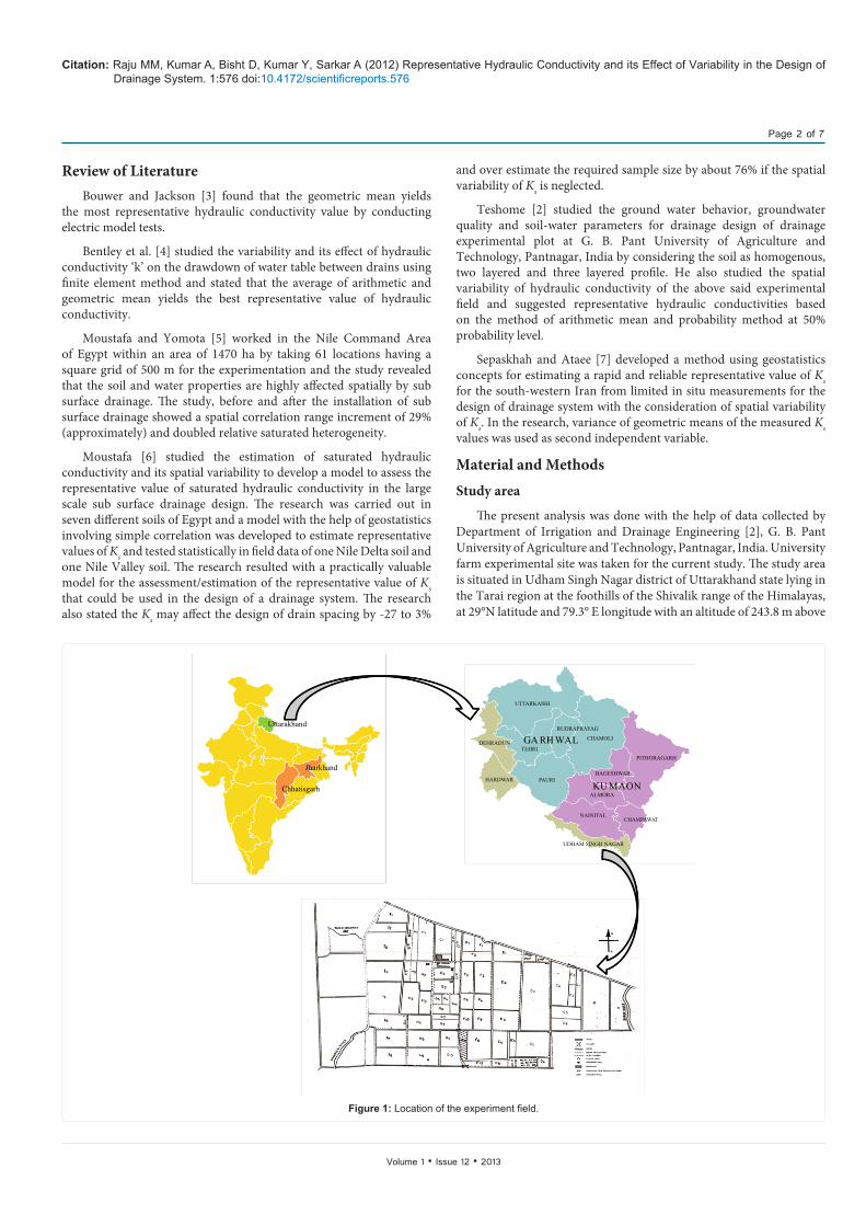
The present analysis was done with the help of data collected by Department of Irrigation and Drainage Engineering [2], G. B. Pant University of Agriculture and Technology, Pantnagar, India. University farm experimental site was taken for the current study. The study area is situated in Udham Singh Nagar district of Uttarakhand state lying in the Tarai region at the foothills of the Shivalik range of the Himalayas, at 29°N latitude and 79.3° E longitude with an altitude of 243.8 m above

Uttarakhand

DEHRADUN

UTTARKASHI

RUDRAPRAYAG

TEHRI

PAURIHARDWAR

CHAMOLI

PITHORAGARH

BAGESHWAR

ALMORA

NAINITALCHAMPAWAT

UDHAM SINGH NAGAR

GA RH WAL

KU MAON

Jharkhand

Chhatisgarh

Figure 1: Location of the experiment field.



Page 3 of 7


mean sea level. The climate is humid and subtropical of an average annual rainfall of 1400 mm. The experimental field was surrounded by drainage along the south, by a river in the west, by cultivated land in the east, and by a farm road in the north. The area of the site was 2.5 ha and it had not been under cultivation for several years because of water logging problem. During the month of December, it was even difficult to enter the farm machinery into the field (Figure 1).

The present chapter deals with the generally used drainage design steady state (homogeneous soil profile) solutions and unsteady state (homogeneous soil profile) solutions.

Determination of representative hydraulic conductivity

The methods used to obtain representative hydraulic conductivity in the present study were geometric mean, average of arithmetic mean and geometric mean, Weibull distribution plotting positions at 50% and 80% level. The plotting position for the Weibull distribution was given by

( 1)=

+mP

N (1)

Where

P=probability of occurrence of ‘k’ corresponding to rank ‘m’

m=rank number in the descending order of ‘k’ values

N=total number of ‘k’ values obtained in the field

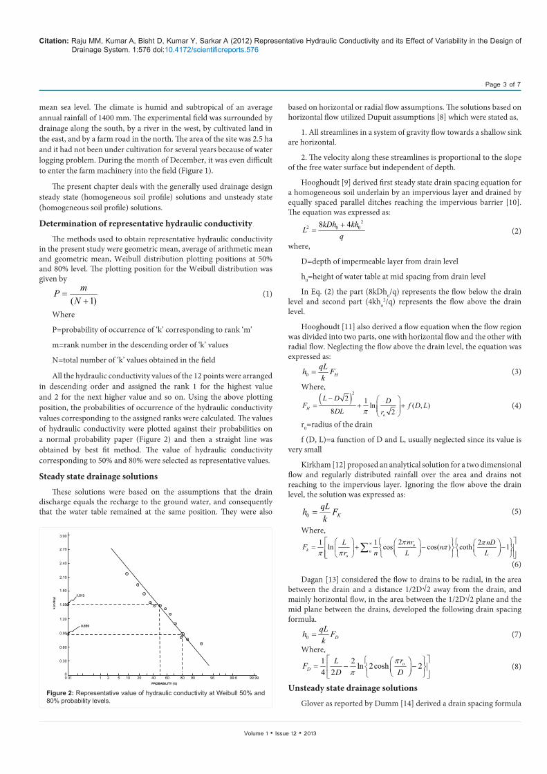
All the hydraulic conductivity values of the 12 points were arranged in descending order and assigned the rank 1 for the highest value and 2 for the next higher value and so on. Using the above plotting position, the probabilities of occurrence of the hydraulic conductivity values corresponding to the assigned ranks were calculated. The values of hydraulic conductivity were plotted against their probabilities on a normal probability paper (Figure 2) and then a straight line was obtained by best fit method. The value of hydraulic conductivity corresponding to 50% and 80% were selected as representative values.

Steady state drainage solutions

These solutions were based on the assumptions that the drain discharge equals the recharge to the ground water, and consequently that the water table remained at the same position. They were also

based on horizontal or radial flow assumptions. The solutions based on horizontal flow utilized Dupuit assumptions [8] which were stated as,

1. All streamlines in a system of gravity flow towards a shallow sink are horizontal.

2. The velocity along these streamlines is proportional to the slope of the free water surface but independent of depth.

Hooghoudt [9] derived first steady state drain spacing equation for a homogeneous soil underlain by an impervious layer and drained by equally spaced parallel ditches reaching the impervious barrier [10]. The equation was expressed as:

22 0 08 4+

=kDh kh

Lq (2)

where,

D=depth of impermeable layer from drain level

h0=height of water table at mid spacing from drain level

In Eq. (2) the part (8kDho/q) represents the flow below the drain level and second part (4kho

2/q) represents the flow above the drain level.

Hooghoudt [11] also derived a flow equation when the flow region was divided into two parts, one with horizontal flow and the other with radial flow. Neglecting the flow above the drain level, the equation was expressed as:

0 = HqLh Fk

(3)

Where,( )2

2 1 ln ( , )8 2π

− = + +

H

o

L D DF f D LDL r

(4)

r0=radius of the drain

f (D, L)=a function of D and L, usually neglected since its value is very small

Kirkham [12] proposed an analytical solution for a two dimensional flow and regularly distributed rainfall over the area and drains not reaching to the impervious layer. Ignoring the flow above the drain level, the solution was expressed as:

0 = KqLh Fk

(5)

Where,21 1 2ln cos cos( ) coth 1π ππ

π π∞ = + − −

∑ ok n

o

nrL nDF nr n L L

(6)

Dagan [13] considered the flow to drains to be radial, in the area between the drain and a distance 1/2D√2 away from the drain, and mainly horizontal flow, in the area between the 1/2D√2 plane and the mid plane between the drains, developed the following drain spacing formula.

0 = DqLh Fk

(7)

Where, 1 2 ln 2cosh 24 2

ππ

= − −

oD

rLFD D

(8)

Unsteady state drainage solutions

Glover as reported by Dumm [14] derived a drain spacing formula

.

.

.

. ..

.

...

.

.. .

.

3.00

2.70

2.40

2.10

1.80

1.50

1.20

0.90

0.60

0.30

00 01 1 2 5 10 20 40 60 80 90 96 99.6 99.99

PROBABILITY (%)

1.513

0.859

k (m

/day

)

Figure 2: Representative value of hydraulic conductivity at Weibull 50% and 80% probability levels.



Page 4 of 7


for unsteady state flow between two parallel ditches from the following differential equation.

2

2 µ∂ ∂=

∂∂h hkD

tx (9)

where,

kD=transmissivity of the aquifer

x=horizontal distance from a reference point (e.g. ditch)

μ=drainable pore space

t=time

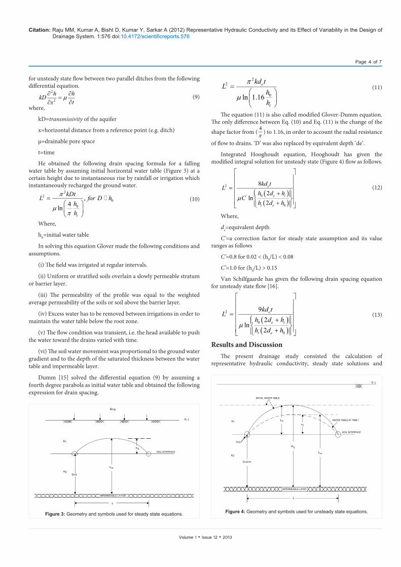
He obtained the following drain spacing formula for a falling water table by assuming initial horizontal water table (Figure 3) at a certain height due to instantaneous rise by rainfall or irrigation which instantaneously recharged the ground water.

22

00

,4ln

π

µπ

= t

kDtL for D hhh

� (10)

Where,

h0=initial water table

In solving this equation Glover made the following conditions and assumptions.

(i) The field was irrigated at regular intervals.

(ii) Uniform or stratified soils overlain a slowly permeable stratum or barrier layer.

(iii) The permeability of the profile was equal to the weighted average permeability of the soils or soil above the barrier layer.

(iv) Excess water has to be removed between irrigations in order to maintain the water table below the root zone.

(v) The flow condition was transient, i.e. the head available to push the water toward the drains varied with time.

(vi) The soil water movement was proportional to the ground water gradient and to the depth of the saturated thickness between the water table and impermeable layer.

Dumm [15] solved the differential equation (9) by assuming a fourth degree parabola as initial water table and obtained the following expression for drain spacing.

22

0ln 1.16

π

µ=

e

t

kd tL

hh

(11)

The equation (11) is also called modified Glover-Dumm equation. The only difference between Eq. (10) and Eq. (11) is the change of the

shape factor from ( 4π

) to 1.16, in order to account the radial resistance

of flow to drains. ‘D’ was also replaced by equivalent depth ‘de’.

Integrated Hooghoudt equation, Hooghoudt has given the modified integral solution for unsteady state (Figure 4) flow as follows.

( )( )

2

0'

0

82

ln2

µ

= + +

e

e t

t e

kd tL

h d hC

h d h

(12)

Where,

de=equivalent depth

C’=a correction factor for steady state assumption and its value ranges as follows

C’=0.8 for 0.02 < (h0/L) < 0.08

C’=1.0 for (h0/L) > 0.15

Van Schilfgaarde has given the following drain spacing equation for unsteady state flow [16].

( )( )

2

0

0

92

ln2

µ

= + +

e

e t

t e

kd tL

h d hh d h

(13)

Results and DiscussionThe present drainage study consisted the calculation of

representative hydraulic conductivity, steady state solutions and

R=q

K1

K2

G. L

SOIL INTERFACE

D=d

h m

h 0

L

IMPERMEA BLE LA YER

Figure 3: Geometry and symbols used for steady state equations.

H

G. L

INITIAL WATER TABLE

WATER TABLE AT TIME t

SOIL INTERFACE

TILE

K1

K2

D=d=H

IMPERMEABLE LAYER

L

h m

h t

h 0

0

Figure 4: Geometry and symbols used for unsteady state equations.



Page 5 of 7


S. No Location Hydraulic conductivity (k)

Geometric mean of ‘k’

Average of arithmetic and geometric mean of ‘k’

k at 50% weibull probability level

k at 80% weibull probability level

1 B3 1.598

1.342 1.381 1.513 0.859

2 F3 1.7913 B9 1.1774 F9 1.5515 B13 0.8826 F13 0.8257 B18 1.4758 F18 1.9709 B22 1.56310 F22 1.37111 B27 0.67012 F27 2.158

Table 1: Hydraulic conductivities of different locations of experimental field.

S. No EquationsHydraulic

conductivity (m/day)

Spacing (m)q=0.02 m/day

% variation in spacing with respect to spacing with arithmetic mean ‘k’

Spacing (m)q=0.007 m/

day

% variation in spacing with respect to spacing with

arithmetic mean ‘k’Remarks

1

Hooghoudt (1937)1

22 0 08 4+

=kDh kh

Lq

kgm=1.342kagm=1.381k50%=1.513k80%=0.859

14.2014.3915.0711.35

-2.61-1.30+3.36-22.15

24.0024.3325.4619.20

-2.60-1.26+3.33-22.10

2Hooghoudt (1940)

0 = H

qLh Fk

kgm=1.342kagm=1.381k50%=1.513k80%=0.859

11.3011.2111.748.70

-19.86-20.50-16.74-38.3

19.0419.3220.2515.16

-21.20-20.00-61.15-37.22

FH = 2.970/5.034FH = 3.070/5.105FH = 3.220/5.336FH = 2.460/4.050

3Kirkham (1958)

0 = K

qLh Fk

kgm=1.342kagm=1.381k50%=1.513k80%=0.859

11.1211.2511.848.68

-1.160.00

+5.24-22.84

19.6019.8820.8715.39

+0.77+2.21+7.30-20.87

FK = 3.017/4.890FK = 3.060/4.962FK = 3.194/5.178FK = 2.474/3.986

4Dagan (1965)

0 = D

qLh Fk

kgm=1.342kagm=1.381k50%=1.513k80%=0.859

10.8612.5113.158.60

-3.04+11.70+17.41-23.21

18.8620.6121.5014.90

-2.78+6.24

+10.82-23.20

FD = 3.089/5.083FD = 2.759/4.781FD = 2.876/5.026FD = 2.500/4.120

Table 2: Steady state drain spacing solutions using different representative hydraulic conductivities.

S. No Equations Hydraulic conductivity (m/day) Spacing (m) % variation in spacing with respect to spacing with arithmetic mean ‘k’ Remarks

1

Glover (1954)2

20

ln(1.27 )= e

t

kd tL

hh

π

µ

kgm=1.342kagm=1.381k50%=1.513k80%=0.859

18.7018.9319.8114.93

+0.54+1.77+6.50-19.73

de=0.490de=0.490de=0.490de=0.490

2

Glover – Dumm (1960)

22

0

ln(1.16 )= e

t

kd tL

hh

π

µ

kgm=1.342kagm=1.381k50%=1.513k80%=0.859

19.8420.2021.1015.87

-0.30+1.51+6.03-20.25

de=0.490de=0.491de=0.492de=0.490

3

Integrated Hooghoudt (1963)

2 e

0

0

8 d t(2 )

' ln(2 )

= + +

e t

t e

kL

h d hC

h d hµ

kgm=1.342kagm=1.381k50%=1.513k80%=0.859

25.0032.0033.3225.24

+7.07+37.04+42.70+8.09

de=0.490de=0.500de=0.500de=0.490

4

Van Schilfgaarde (1964)

2 e

0

0

9 d t(2 )

ln(2 )

= + +

e t

t e

kL

h d hh d h

µ

kgm=1.342kagm=1.381k50%=1.513k80%=0.859

31.5030.3631.7723.81

+3.80+0.03+4.70-21.55

de=0.500de=0.500de=0.500de=0.490

Table 3: Unsteady state drain spacing solutions using different representative hydraulic conductivities.



Page 6 of 7


unsteady state solutions by considering the soil profile as homogeneous, isotropic upto a depth 150cm below the ground level. In the method of calculation of representative hydraulic conductivity statistical methods like geometric mean, average of arithmetic and geometric mean and Weibull probability distribution method plotting positions at 50% and 80% level were adopted (Table 1). The common parameters for the steady state were taken as D=0.5m, r0=0.05 m, h0=0.5 m and for unsteady state as h0=1.20 m, ht=0.70 m, r0=0.1 m, t=2 days and μ=0.048. The drainage coefficient 0.02 m/day suggested by Sewa Ram [1] for Tarai region of Uttarakhand and the most generalized drainage coefficient 0.007 m/day suggested by International Institute for Land Reclamation and Improvement, Wageningen, The Netherlands for most of the selected equations under all conditions were used in the study of steady state solutions. The representative hydraulic conductivities used in this study were 1.342 (geometric mean), 1.381 (average of arithmetic mean and geometric mean), 1.513 (probability method at 50% level), and 0.859 (probability method at 80% level).

In the steady state drainage design [9,11-13] theories and in the unsteady state drainage design Glover, Dumm [15], Integrated Hooghoudt (1963) and Schilfgaarde [16] theories were used for drainage spacing calculations. Wide spacings were obtained by Hooghoudt [9] and narrow spacings were obtained by Hooghoudt, Kirkham and Dagan theories in steady state drainage design [11-13] (Table 2), whereas in the case of unsteady state drainage design wide spacings were obtained by Integrated Hooghoudt (1963) and Van Schilfgaarde [16] theories and narrow spacings were obtained by Glover (1954) and Glover-Dumm [15] theories (Table 3).

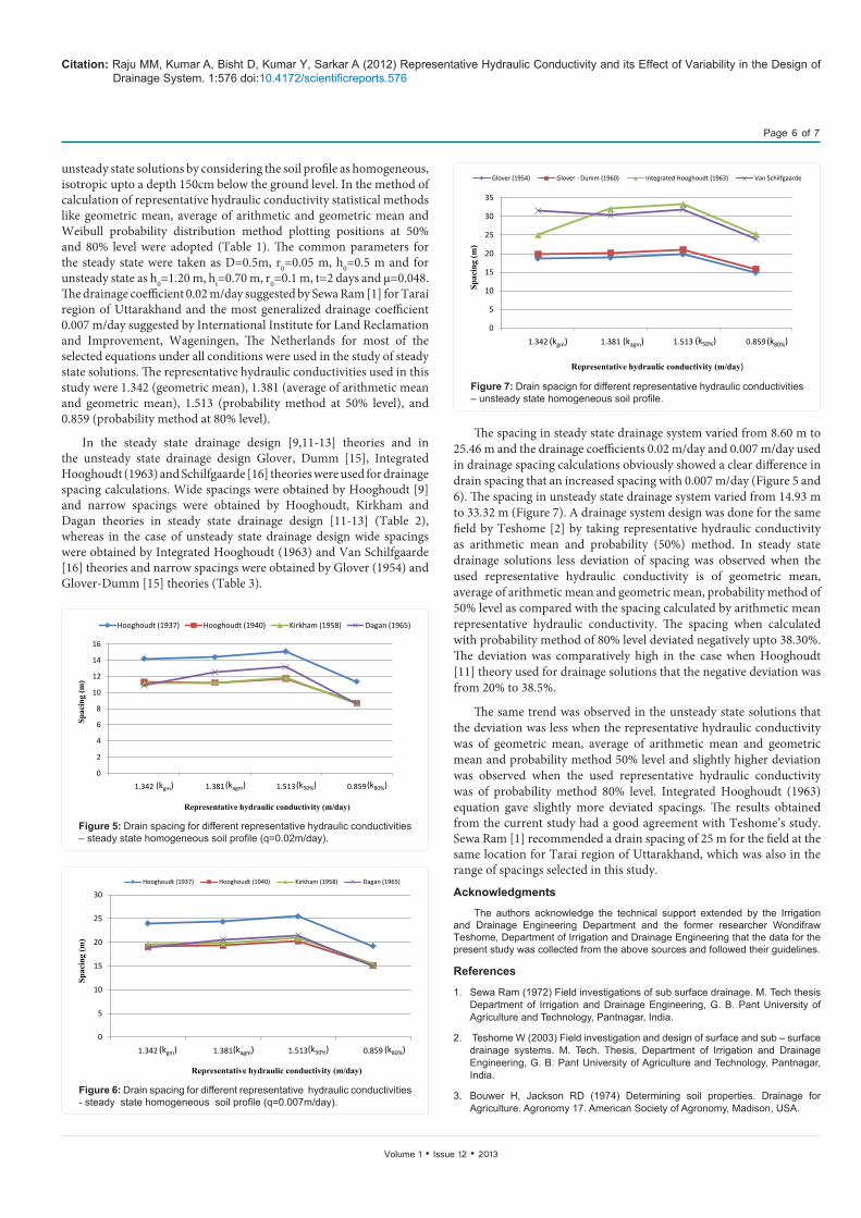
The spacing in steady state drainage system varied from 8.60 m to 25.46 m and the drainage coefficients 0.02 m/day and 0.007 m/day used in drainage spacing calculations obviously showed a clear difference in drain spacing that an increased spacing with 0.007 m/day (Figure 5 and 6). The spacing in unsteady state drainage system varied from 14.93 m to 33.32 m (Figure 7). A drainage system design was done for the same field by Teshome [2] by taking representative hydraulic conductivity as arithmetic mean and probability (50%) method. In steady state drainage solutions less deviation of spacing was observed when the used representative hydraulic conductivity is of geometric mean, average of arithmetic mean and geometric mean, probability method of 50% level as compared with the spacing calculated by arithmetic mean representative hydraulic conductivity. The spacing when calculated with probability method of 80% level deviated negatively upto 38.30%. The deviation was comparatively high in the case when Hooghoudt [11] theory used for drainage solutions that the negative deviation was from 20% to 38.5%.

The same trend was observed in the unsteady state solutions that the deviation was less when the representative hydraulic conductivity was of geometric mean, average of arithmetic mean and geometric mean and probability method 50% level and slightly higher deviation was observed when the used representative hydraulic conductivity was of probability method 80% level. Integrated Hooghoudt (1963) equation gave slightly more deviated spacings. The results obtained from the current study had a good agreement with Teshome’s study. Sewa Ram [1] recommended a drain spacing of 25 m for the field at the same location for Tarai region of Uttarakhand, which was also in the range of spacings selected in this study.

Acknowledgments

The authors acknowledge the technical support extended by the Irrigation and Drainage Engineering Department and the former researcher Wondifraw Teshome, Department of Irrigation and Drainage Engineering that the data for the present study was collected from the above sources and followed their guidelines.

References

1. Sewa Ram (1972) Field investigations of sub surface drainage. M. Tech thesis Department of Irrigation and Drainage Engineering, G. B. Pant University of Agriculture and Technology, Pantnagar, India.

2. Teshome W (2003) Field investigation and design of surface and sub – surface drainage systems. M. Tech. Thesis, Department of Irrigation and Drainage Engineering, G. B. Pant University of Agriculture and Technology, Pantnagar, India.

3. Bouwer H, Jackson RD (1974) Determining soil properties. Drainage for Agriculture. Agronomy 17. American Society of Agronomy, Madison, USA.

0

2

4

6

8

10

12

14

16

1.342 1.381 1.513 0.859

Hooghoudt (1937) Hooghoudt (1940) Kirkham (1958) Dagan (1965)

Spac

ing

(m)

(kgm)

Representative hydraulic conductivity (m/day)

(kagm) (k50%) (k80%)

Figure 5: Drain spacing for different representative hydraulic conductivities – steady state homogeneous soil profile (q=0.02m/day).

0

5

10

15

20

25

30

1.342 1.381 1.513 0.859

Hooghoudt (1937) Hooghoudt (1940) Kirkham (1958) Dagan (1965)

Spac

ing

(m)


(kgm) (kagm) (k50%) (k80%)

Figure 6: Drain spacing for different representative hydraulic conductivities - steady state homogeneous soil profile (q=0.007m/day).

0

5

10

15

20

25

30

35

1.342 1.381 1.513 0.859

Glover (1954) Glover - Dumm (1960) Integrated Hooghoudt (1963) Van Schilfgaarde


Spac

ing

(m)

(kgm) (kagm) (k50%) (k80%)

Figure 7: Drain spacign for different representative hydraulic conductivities – unsteady state homogeneous soil profile.



Page 7 of 7


4. Bentley WJ, Skaggs RW, Parsons JE (1989) The effect of variation in hydraulic conductivity on water table drawdown. Technical bulletin, North Corolina Agricultural Research Service, North Corolina State University, Releigh, NC, USA.

5. Moustafa MM, Yomota A (1998) Use of a covariance variogram to investigate influence of subsurface drainage on spatial variability of soil-water properties. Agricultural Water Management 37: 1-19.

6. Moustafa MM (2000) A geostatistical approach to optimize the determination of saturated hydraulic conductivity for large-scale subsurface drainage design in Egypt. Agr Water Manage 42: 291-312.

7. Sepaskhah AR, Ataee J (2004) A Simple Model to determine Saturated Hydraulic Conductivity for Large-scale Subsurface Drainage. Biosystems Engineering 89: 505-513.

8. Luthin, JN (1970) Drainage Engineering, Wiley Eastern Private Limited, New Delhi, India.

9. Hooghoudt SB (1937) Contributions to the knowledge of some physical quantities of the ground, Determination of permeability in soils of the second sort, theory and application of quantitative inundation of water in shallow aquifers, particularly in relation to drainage and infiltration issues. Encrypt Landb, Ent. Algemeene country printing, The Hauge 43: 515-707.

10. Van der Ploeg RR, Kirkham MB, Marquardt M (1999) The Colding Equation for Soil Drainage: Its Origin, Evolution, and Use. Soil Science Society Am Journal 63: 33-39.

11. Hooghoudt SB (1940) Contributions to the knowledge of some physical quantities of the ground, Algemeene consideration of the problem of detailed drainage and infiltration by the middle of parallel loop income drains, ditches, canals and ditches. Encrypt Landb, Ent Algemeene Country Printing, The Hauge 46: 515-707.

12. Kirkham D (1958) Seepage of steady rainfall through soil into drains. Transactions of American Geophysics Union 39: 892-908.

13. Dagan G (1965) Steady drainage of a two-layered soil. Journal of Irrigation and Drainage Division, Proceedings of the ASCE 91: 51–64.

14. Dumm LD (1954) Drain spacing formula: New formula for determining depth and spacing of subsurface drins in irrigated lands. Agr Eng 10: 726–730.

15. Dumm LD (1960) Validity and Use of the Transient-flow Concept in Subsurface Drainage. American Society of Agricultural Engineers, USA.

16. Schilfgaarde JV (1963) Design of tile drainage for falling water tables. Journal of Irrigation and Drainage Division 89: 1-12.

http://books.google.co.in/books/about/The_Effect_of_Variation_in_Hydraulic_Con.html?id=g5uMtgAACAAJ&redir_esc=y

http://www.sciencedirect.com/science/article/pii/S0378377498000468



https://www.soils.org/publications/sssaj/abstracts/63/1/SS0630010033

http://books.google.co.in/books/about/Validity_and_Use_of_the_Transient_flow_C.html?id=qnWlGwAACAAJ&redir_esc=y

http://cedb.asce.org/cgi/WWWdisplay.cgi?12933


irrigation & drainage systems engineering · irrigation, drainage, engineering hydrology, and...

Documents