IO FOR EXPORT(S)∗

Monika Mrazova†

University of Geneva,

CEPR and CESifo

J. Peter Neary‡

University of Oxford,

CEPR and CESifo

October 1, 2019

Abstract

We provide an overview and synthesis of recent work on models of monopolistic

competition with heterogeneous firms in international trade, paying particular atten-

tion to competition effects, pass-through, selection effects, and linking distributions of

firm characteristics and outcomes. A recurring theme is that CES preferences are ex-

tremely convenient for deriving analytic results, but also extremely restrictive in their

theoretical and empirical implications. We introduce the class of “constant-response

demand functions” to describe some related families of demand functions that provide

a unifying principle for much recent work that explores alternatives to CES demands.

Keywords: Heterogeneous Firms; Pass-Through; Quantifying Effects of Globalization; Super- and

Sub-Convexity; Supermodularity.

JEL Classification: F12, L11, F23

∗This is a revised version of a plenary lecture presented at EARIE 2018, the 45th Annual Conference ofthe European Association for Research in Industrial Economics, Athens, September 2018. We are gratefulto participants on that occasion, at the Research Workshop on International Trade in Villars, Switzerland,the 2019 IEE Research Day in Geneva, a conference on International Economic Integration in Tubingen, the2019 CESifo Area Conference on Global Economy in Munich, ERWIT 2019 in London, SAET 2019 in Ischia,the 2019 Hitotsubashi Summer Institute in Tokyo, ETSG 2019 in Bern, and a seminar at University CollegeDublin. We also thank the editor, Paul Heidhues, two referees, Paolo Bertoletti, Luis Cabral, ToshihiroOkubo and John Vickers, for helpful comments and discussions. Monika Mrazova thanks the Fondation deFamille Sandoz for funding under the “Sandoz Family Foundation - Monique de Meuron” Programme forAcademic Promotion. Peter Neary thanks the European Research Council for funding under the EuropeanUnion’s Seventh Framework Programme (FP7/2007-2013), ERC grant agreement no. 295669.†Geneva School of Economics and Management (GSEM), University of Geneva, Bd. du Pont d’Arve 40,

1211 Geneva 4, Switzerland; e-mail: monika.mrazova@unige.ch.‡Department of Economics, University of Oxford, Manor Road, Oxford OX1 3UQ, UK; e-mail: pe-

ter.neary@economics.ox.ac.uk.

1 Introduction

In this paper we aim to provide an overview of recent research in international trade, from the

perspective of the theory of industrial organization (henceforth IO). There are two aspects to

this perspective, mirroring the two different interpretations of our title. On the one hand, we

are interested in “IO for Exports”: what is the structure of export markets?; how does that

structure affect which firms export?; does trade fosters competition?; and a host of other

similar questions. On the other hand, we want to think about “IO for Export”: which IO

models are used in trade? As is well-known, the answer to the latter question is not any of

the many varieties of oligopoly used in IO itself, but rather the monopolistically competitive

model of Chamberlin (1933), as formalized by Dixit and Stiglitz (1977); especially with

Constant-Elasticity-of-Substitution (CES) preferences, introduced as a special case by Dixit

and Stiglitz (1977), brought to center stage by Dixit and Norman (1980) and Krugman

(1980) among many others, and extended to firm heterogeneity by Melitz (2003). Ironically,

though monopolistic competition originated in IO, it is used relatively rarely there, so it

could be described as “IO for export only.”1

While monopolistic competition is by far the dominant paradigm in international trade,

it is by no means the only approach. First there is a large literature on “strategic” trade

policy, dating from the 1980s, that uses off-the-shelf IO models of oligopoly to address

standard issues of trade policy, mostly at the level of a single industry.2 Second, there

have been some attempts to explore the implications of oligopoly in general equilibrium for

trade questions, both of the traditional kind such as trade patterns, gains from trade and

pricing-to-market,3 and also with applications to topics such as cross-border mergers and

1See Neary (2003b) for further discussion. Of course, studies of monopolistic competition, in both CESand non-CES cases, are not completely absent from IO. Examples include advanced textbook treatments byAnderson et al. (1992) and Vives (1999), as well as studies of existence by Pascoa (1993) and Pascoa (1997),and of optimality by Kuhn and Vives (1999).

2See Brander (1995) for an overview, and Mrazova (2011) and Mrazova et al. (2013), for applications totrade agreements.

3See, for example, Neary (2003a), Atkeson and Burstein (2008), Neary (2016), Gaubert and Itskhoki(2018), and Nocke and Schutz (2018).

multi-product exporters.4 Finally, there is a small literature on the theory of superstar firms

that compete oligopolistically, while coexisting with a monopolistically competitive fringe.5

However, there are good reasons why the monopolistically competitive paradigm has

remained dominant in trade. The availability of large data sets on exporting firms, and

the desire to allow for entry and exit and to take account of general-equilibrium feedbacks

to and from factor markets, make bespoke modelling of individual sectors infeasible, and a

“one-size-fits-all” approach to the choice of market structure very convenient.

Two general themes emerge from our analysis, one old, one new. First, the widespread

assumption of CES preferences, implying demand functions that are log-linear in price,

is extremely convenient for deriving analytic results, but also extremely restrictive in its

theoretical and empirical implications. Second, we introduce the class of “constant-response

demand functions” to describe some related families of parametric demand functions that

imply a constant absolute or relative response of some firm-level variable to an exogenous

change in marginal cost. As we shall see, this class of demands, all of which nest the CES

case, provides a unifying principle for much recent work, including our own, that explores

alternatives to CES demands.6

The plan of the paper is as follows. Section 2 introduces the basic underlying model

and an approach to comparing different demand functions that we use throughout. It also

discusses recent evidence that questions a key implication of CES preferences. Each of the

four subsequent sections considers a substantive question, and asks, which demand functions

arise naturally in trying to answer it? As we show, each question can be formulated in

terms of a constant response of a target function to a change in costs, and so we are led

to seeking demand functions that are consistent with such a constant response. Section 3

considers the central topic of competition effects, and shows that the CES demand function

4See, for example, Neary (2007), Eckel and Neary (2010) and Eckel et al. (2015).5See, for example, Neary (2010), Shimomura and Thisse (2012), Parenti (2018), and Cabral (2018).6For other approaches to going “beyond CES,” see Zhelobodko et al. (2012), Bertoletti and Epifani (2014),

Parenti et al. (2017), Dhingra and Morrow (2019), and Matsuyama and Ushchev (2017). For the most part,these papers consider non-parametric families of demand functions, whereas in this paper we focus on familieswith explicit functional forms.

3

is a key benchmark in categorizing them, both at the firm level in the cross-section and in

general equilibrium when the economy responds to exogenous shocks. Section 4 considers

the issue of how cost changes are passed through to goods prices, and introduces the Bulow-

Pfleiderer (B-P) and Constant-Proportional-Pass-Through (CPPT) demand functions that

correspond to constant rates of absolute and proportional pass-through respectively. Sec-

tion 5 turns to consider the central topic of selection effects, and introduces the Constant-

Elasticity-of-Marginal-Revenue (CEMR) demand functions that provide a natural reference

point for understanding them. Section 6 explores the relationship between the distribution

of firm productivity, on the one hand, and the distributions of the level and growth rate of

sales, on the other; and it introduces the Constant-Revenue-Elasticity-of-Marginal-Revenue

(CREMR) demand functions that arise naturally in this context. Finally, Section 7 provides

an overview of the constant-response demand functions introduced in earlier sections, and

introduces a general demand function that nests three of them. Section 8 concludes. Proofs

and further details can be found in our other papers: Mrazova and Neary (2017) for Sec-

tions 2, 3 and 4, Mrazova and Neary (2019) for Section 5, and Mrazova et al. (2015) for

Section 6.

2 Preliminaries

2.1 A Core Model

We begin by presenting a simple core model of a monopoly firm. This serves to introduce

the notation and setting that we will use throughout the remainder of the paper.

Consider a monopoly firm facing an inverse demand function p(x), giving price as a

strictly decreasing function of firm output x. This is consistent with monopolistic competi-

tion where the firm takes the “perceived” demand function as given. In general equilibrium,

the demand function has extra arguments: we will see examples of that later. As for technol-

ogy, we adopt the simplest specification popularized by Dixit and Stiglitz (1977): all firms

4

incur a fixed cost f, often assumed to be constant across firms, and a constant marginal

cost of production c.7 Profit maximization therefore implies simple first- and second-order

conditions:

p+ xp′ = c and 2p′ + xp′′ < 0 (1)

In words, marginal revenue must equal marginal cost, and marginal revenue must be declining

in output at the optimum. It will prove convenient to write these conditions in terms of two

key demand parameters:

ε(x) ≡ − p(x)

xp′(x)> 0 and ρ(x) ≡ −xp

′′(x)

p′(x)(2)

Here ε(x) is the demand elasticity and ρ(x) the convexity of demand; these are unit-free

measures of the slope and curvature of the demand function, respectively. Reexpressing the

first- and second-order conditions in (1) in terms of these parameters yields, first, a simple

expression linking the price-cost margin or markup, p/c, to the elasticity of demand, and,

second, a restriction that convexity must be less than two:

p

c=

ε

ε− 1and ρ < 2 (3)

2.2 Demand Functions and Demand Manifolds

Throughout the paper, we will see many different parametric forms of demand function, and

it is desirable to have some way of comparing them. As is foreshadowed in the previous

section, for many questions of interest only the elasticity and convexity of demand matter.

Hence it makes sense, following Mrazova and Neary (2017), to illustrate different demand

7Dixit and Stiglitz should not be held responsible for the widespread use of CES preferences: theypresented them only as an example, albeit with the unique implication of constrained efficiency (see theirSection I), and each of them is on record as expressing reservations about them: see Dixit (2004) and Stiglitz(2004). However, they deserve credit for popularizing, and perhaps making respectable, the very simplef, c technology. Ironically, this is another example of IO for export only: it is now ubiquitous in trade,whereas more complicated cost functions are often used in the IO literature.

5

0.0

1.0

2.0

3.0

4.0

-2.0 -1.0 0.0 1.0 2.0 3.0

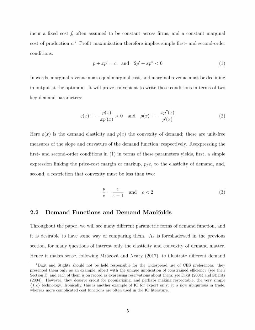
Figure 1: The Admissible Region in Convexity-Elasticity Space

functions in the space of these two parameters, as in Figure 1. The shaded area represents

the admissible region implied by the restrictions in equation (3): at a profit-maximising

equilibrium, a monopoly firm must be at a point on its demand function where the elasticity

is greater than one, and the convexity is less than two.8

The space illustrated in Figure 1 may seem unfamiliar at first, so it is desirable to have

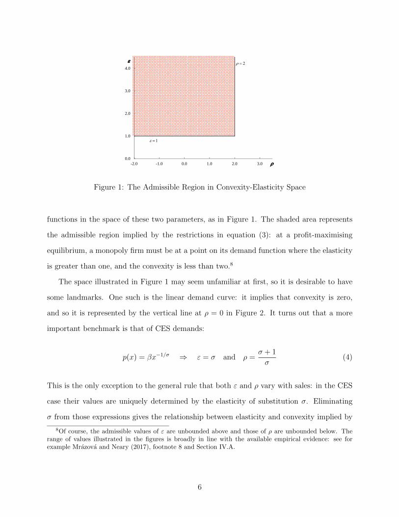
some landmarks. One such is the linear demand curve: it implies that convexity is zero,

and so it is represented by the vertical line at ρ = 0 in Figure 2. It turns out that a more

important benchmark is that of CES demands:

p(x) = βx−1/σ ⇒ ε = σ and ρ =σ + 1

σ(4)

This is the only exception to the general rule that both ε and ρ vary with sales: in the CES

case their values are uniquely determined by the elasticity of substitution σ. Eliminating

σ from those expressions gives the relationship between elasticity and convexity implied by

8Of course, the admissible values of ε are unbounded above and those of ρ are unbounded below. Therange of values illustrated in the figures is broadly in line with the available empirical evidence: see forexample Mrazova and Neary (2017), footnote 8 and Section IV.A.

6

CES demands:

ε =1

ρ− 1(5)

This relationship is illustrated by the curve labelled “CES” in Figure 2; it ranges from an

asymptotically infinite value of ε as ρ approaches one to a value of ε equal to one when ρ

equals two. Each point on this curve represents a particular CES demand function corre-

sponding to a particular value of σ; for example, the point ρ = 2, ε = 1, just on the

boundary of the admissible region, corresponds to the Cobb-Douglas special case.

0.0

1.0

2.0

3.0

4.0

-2.0 -1.0 0.0 1.0 2.0 3.0

Linear

CARA

LES

CES

Translog

Figure 2: Demand Manifolds for Some Common Demand Functions

The linear and CES demand functions are not the only ones that can be illustrated in

(ρ, ε)-space. As shown in Mrazova and Neary (2017), any demand function can be illustrated

in this space by a smooth curve, which they call the “demand manifold” corresponding to

the demand function. (The only exception is CES demands, where as we have seen the

manifold is a single point.) Figure 2 illustrates the manifolds for three other widely-used

demand functions: the negative exponential or CARA (“constant absolute risk-aversion”)

system, the Stone-Geary LES (“linear expenditure system”), and the translog (which from a

firm’s perspective is observationally equivalent to the “Almost Ideal” system of Deaton and

7

Muellbauer (1980)).9 (Explicit expressions are in Appendix B.)

There are a number of advantages to considering demand functions through the lens

of their manifolds. First, different demand functions can be directly compared with each

other. For example, Figure 2 shows that, despite their very different origins and system-

wide properties, all three of CARA, LES and translog demands have properties at the firm

level that are midway between those of linear and CES demands. In particular, for a given

demand elasticity they are all less convex than CES demands, though they are more so than

linear demands.

Second, demand manifolds make it possible to relate assumptions about demand directly

to comparative statics properties: we will see examples of this later. Finally, though the

location of a demand function in (x, p)-space is affected by the values of all its parameters,

the location of its manifold in (ρ, ε)-space is often unaffected by, or invariant to, the values of

these parameters. Mrazova and Neary (2017) call this property “manifold invariance”, and

provide necessary and sufficient conditions for it to hold. Not all demand functions exhibit

this property with respect to some of their parameters, far less to all of them. The latter is

true of the CES for example: the CES point-manifold is invariant with respect to changes in

the level parameter β but not to changes in the elasticity of substitution σ. However, many

demand functions have manifolds that are invariant to some of their parameters, and some

(including all those other than the CES in Figure 2) have manifolds that are invariant to

all of them. This makes it much easier to think about the implications of different demand

assumptions using the demand manifold than the demand function itself, since the latter is

never invariant to any parameter changes.

9The non-CES demand functions whose manifolds are shown in Figure 2 have been explored in monopo-listic competition with heterogeneous firms by a number of authors. Melitz and Ottaviano (2008) considerlinear demands; Behrens and Murata (2007) CARA demands; Simonovska (2015) the LES; and Feenstraand Weinstein (2017) the translog.

8

2.3 Evidence on Variable Markups

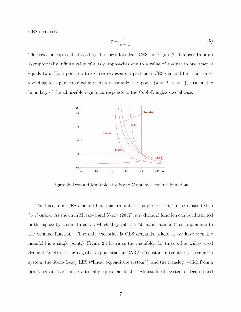
Of the demand functions in Figure 2, the CES is by far the most widely-used in international

trade. However, it makes implausible empirical predictions, in particular that markups

are always the same, and depend only on the preference parameter σ: p/c = σ/(σ − 1).

International trade economists have always been uneasy with these implications, even more

so in recent years as persuasive evidence against them has become available.

PRICES, MARKUPS, AND TRADE REFORM 493

FIGURE 4.—Distribution of marginal costs and markups in 1989 and 1997. Sample only in-cludes firm–product pairs present in 1989 and 1997. Outliers above and below the 3rd and 97thpercentiles are trimmed.

higher markups. The results indicate that firms offset the beneficial cost reduc-tions from improved access to imported inputs by raising markups. The overalleffect, taking into account the average declines in input and output tariffs be-tween 1989 and 1997, is that markups, on average, increased by 12.6 percent.This increase offsets almost half of the average decline in marginal costs, andas a result, the overall effect of the trade reform on prices is moderated.52

Although tempting, it is misleading to draw conclusions about the pro-competitive effects of the trade reform from the markup regressions in Col-umn 3 of Table IX. The reason is that one needs to control for the impacts of

52These results are robust to controlling India’s de-licensing policy reform; see Table A.I in theSupplemental Material.

(a) India, 1989 and 1997 (b) Chile, 2001-2007

Figure 3: Empirical Evidence on Markup DistributionsSources: De Loecker et al. (2016) and Lamorgese et al. (2014)

A key reference is De Loecker et al. (2016), who calculate markups for a sample of Indian

firms without making prior assumptions about market structure or the form of demand.

Figure 3(a) from their paper shows that the distribution of markups is very far from being

concentrated at a single value. A possible explanation is that such markup heterogeneity

arises from aggregation across sectors with different elasticities of substitution. However,

Figure 3(b) from Lamorgese et al. (2014), who use data on Chilean firms, show that hetero-

geneity persists when the data are disaggregated by sector. This evidence clearly rejects the

hypothesis of monopolistic competition with CES preferences. One way to allow for variable

markups is to retain CES preferences but assume an oligopolistic market structure as in

Atkeson and Burstein (2008). In this paper we explore instead how non-CES preferences in

9

monopolistic competition have been used to throw light on a variety of substantive questions

in international trade.

3 Competition Effects

The first substantive topic we wish to discuss is that of competition effects. The term

“competition effects” can be used in two different senses in this context.10 On the one hand,

it can refer to the fact that markups vary across firms in the cross-section. On the other

hand, it can refer to the fact that any exogenous shock to industry equilibrium affects firms

indirectly by changing the competitive environment in which they operate, in addition to its

direct effect on individual firms. As we will see, CES demands are a key reference point for

competition effects in both senses: with CES demands, competition effects do not arise in

the cross section, while, in response to a change in market size, the direct effect of the shock

on firm profits is exactly offset by the induced general-equilibrium competition effect.

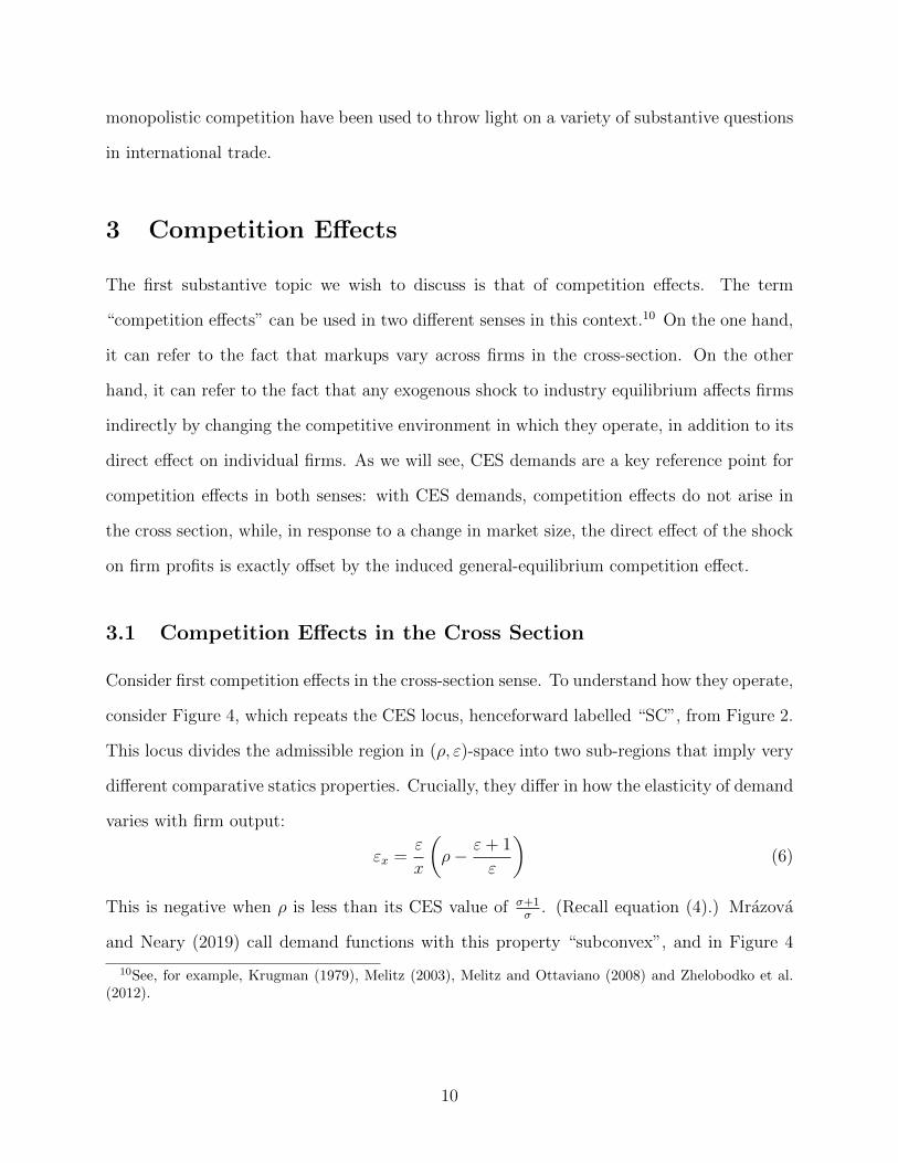
3.1 Competition Effects in the Cross Section

Consider first competition effects in the cross-section sense. To understand how they operate,

consider Figure 4, which repeats the CES locus, henceforward labelled “SC”, from Figure 2.

This locus divides the admissible region in (ρ, ε)-space into two sub-regions that imply very

different comparative statics properties. Crucially, they differ in how the elasticity of demand

varies with firm output:

εx =ε

x

(ρ− ε+ 1

ε

)(6)

This is negative when ρ is less than its CES value of σ+1σ

. (Recall equation (4).) Mrazova

and Neary (2019) call demand functions with this property “subconvex”, and in Figure 4

10See, for example, Krugman (1979), Melitz (2003), Melitz and Ottaviano (2008) and Zhelobodko et al.(2012).

10

0.0

1.0

2.0

3.0

4.0

-2.0 -1.0 0.0 1.0 2.0 3.0

SC

Sub-Convex Super-Convex

Figure 4: The Sub- and Super-Convex Regions

they are represented by the set of points in the region to the left of the SC locus.11 When

the demand curve exhibits this property, larger firms face a lower elasticity of demand and

hence have higher markups in the cross section, and all firms enjoy higher profit margins

as they move down their demand curves over time. (The arrows in the figure indicate how

elasticity changes as firm output rises.) In the converse case, of superconvexity, all these

properties are reversed. However, subconvexity is theoretically more plausible, both on

introspective grounds (see Marshall (1920));12 and also in that it leads to more plausible

predictions (see Dixit and Stiglitz (1977) and Krugman (1979)). Hence we can conclude

that CES demands rule out competition effects, and subconvex demands are necessary and

11Formally, subconvexity is a local property, and is defined as log p(x) being concave in log x at a point.Mrazova and Neary (2019) show that this property is equivalent to those stated in the text. It is possible forthe same demand function, with given parameters, to be subconvex for some levels of output and superconvexfor others. (For an example, see Mrazova and Neary (2017), Online Appendix B10.) However, this propertyis rare, at least as far as most widely-used demand functions is concerned. Moreover, as the argument inthe text shows, the manifold implied by such a demand function must be horizontal at the point where itcrosses the SC locus, since it is falling in output to the left and rising to the right: see the horizontal arrowsin Figure 4.

12In Chapter 3 of Book 4 of his Principles, Marshall introduced his “law of demand” – in modern parlance,demand curves slope downwards – while in Chapter 4 he introduced what he called “the general law ofvariation of the elasticity of demand”: “The elasticity of demand is great for high prices, and great, or atleast considerable, for medium prices; but it declines as the price falls; and gradually fades away if the fallgoes so far that satiety level is reached.” Hence the property is sometimes called “Marshall’s Second Law ofDemand.”

11

sufficient for monopolistic competition to exhibit the empirically plausible case where larger

firms have higher markups.

3.2 Competition Effects of a Globalization Shock

Consider next the second sense of competition effect: the general-equilibrium effect of an

exogenous shock on the competitive environment faced by all firms. An important and

interesting example of this is the effects of globalization, in the sense of an increase in the

size of the global economy.

To see how competition effects arise following a globalization shock, we need to go beyond

the “firm’s eye view” we have adopted so far, and consider the determination of industry

equilibrium.13 Also, since we want to allow for firms to sell in many markets, we distinguish

for the first time between their total output y and the amount they sell to an individual

consumer x. Following Krugman (1979), we take the simplest setting, where all consumers

are identical, there are L of them in each country, and the world consists of k identical

countries, so y = kLx. In addition, though this is not needed for all our results, it is

convenient to assume that preferences are additively separable, so the demand function for a

typical good is given implicitly by the consumer’s first-order condition u′(x) = λp, where λ

is the marginal utility of income.14 With these assumptions, we can write the ex-post profits

of a typical firm as follows:

π(c−, λ−, k

+) ≡ max

y

(p(y, λ, k)− c

)y where p(y, λ, k) = λ−1u′(y/kL) (7)

In previous sections we considered the demand function from a firm’s perspective only. Now

13This section is based on Mrazova and Neary (2017), Section III.B. See also Zhelobodko et al. (2012),Bertoletti and Epifani (2014), Mrazova and Neary (2014), and Bache and Laugesen (2015).

14Writing the demand for each good as p(y, λ, k), a function of its own quantity consumed, a single demand-side aggregate λ, and the exogenous shock k, corresponds to generalized additive separability, introducedby Pollak (1972). Our results, up to and including equation (10) below, hold in this case, though theirinterpretation is simpler when, as in (11), we specialize to additive separability, which implies that λ equalsthe marginal utility of income.

12

we want to solve explicitly for the industry equilibrium, so we need to consider demand

determinants additional to their sales. In (7) these are k, the exogenous globalization shock,

equal to the number of identical countries in the world, and λ, the marginal utility of income

under additive separability, which plays the role of the level of competition in the industry.

This is exogenous to each firm, but is determined endogenously in industry equilibrium by

the free-entry condition, which requires that an entrant has zero expected value. Denoting

by v(λ, k) the expected value of firm profits, this can be written as follows:

v(λ−, k

+) ≡∫ c

c

v(c, λ, k)g(c) dc = fe, v(c, λ, k) ≡ max (0, π(c, λ, k)− f) (8)

Here g(c) is the distribution of firm marginal costs. Prospective firms know this but do not

know their own marginal cost ex ante; to find that out they have to pay a sunk entry cost

fe in order to make a draw from the distribution. This sunk cost must therefore equal the

expected return to sampling from g(c), which with rational expectations and risk neutrality

equals v(λ, k).

We can solve for the effects of globalization on every firm’s profits by totally differentiating

(7):

d log π(c, λ, k)

d log k=∂ log π(c, λ, k)

∂ log k︸ ︷︷ ︸(M)

+∂ log π(c, λ, k)

∂ log λ

d log λ

d log k︸ ︷︷ ︸(C)

(9)

where the change in the level of competition is determined in turn by (8):

d log λ

d log k= −∂ log v(λ, k)

∂ log k

/∂ log v(λ, k)

∂ log λ(10)

Equation (9) shows that globalization is a double-edged sword from the perspective of firms.

On the one hand it has a market-size effect, given by (M), which tends to raise each firm’s

profits. On the other hand it has a competition effect, given by (C): because all firms’ profits

rise at the initial level of competition, the latter must increase to ensure that the expected

value of a firm remains equal to the fixed cost of entry; this in turn tends to reduce each firm’s

13

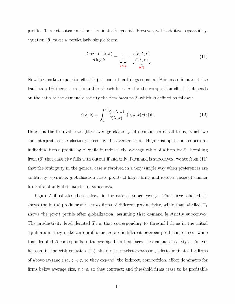
profits. The net outcome is indeterminate in general. However, with additive separability,

equation (9) takes a particularly simple form:

d log π(c, λ, k)

d log k= 1︸︷︷︸

(M)

− ε(c, λ, k)

ε(λ, k)︸ ︷︷ ︸(C)

(11)

Now the market expansion effect is just one: other things equal, a 1% increase in market size

leads to a 1% increase in the profits of each firm. As for the competition effect, it depends

on the ratio of the demand elasticity the firm faces to ε, which is defined as follows:

ε(λ, k) ≡∫ c

c

v(c, λ, k)

v(λ, k)ε(c, λ, k)g(c) dc (12)

Here ε is the firm-value-weighted average elasticity of demand across all firms, which we

can interpret as the elasticity faced by the average firm. Higher competition reduces an

individual firm’s profits by ε, while it reduces the average value of a firm by ε. Recalling

from (6) that elasticity falls with output if and only if demand is subconvex, we see from (11)

that the ambiguity in the general case is resolved in a very simple way when preferences are

additively separable: globalization raises profits of larger firms and reduces those of smaller

firms if and only if demands are subconvex.

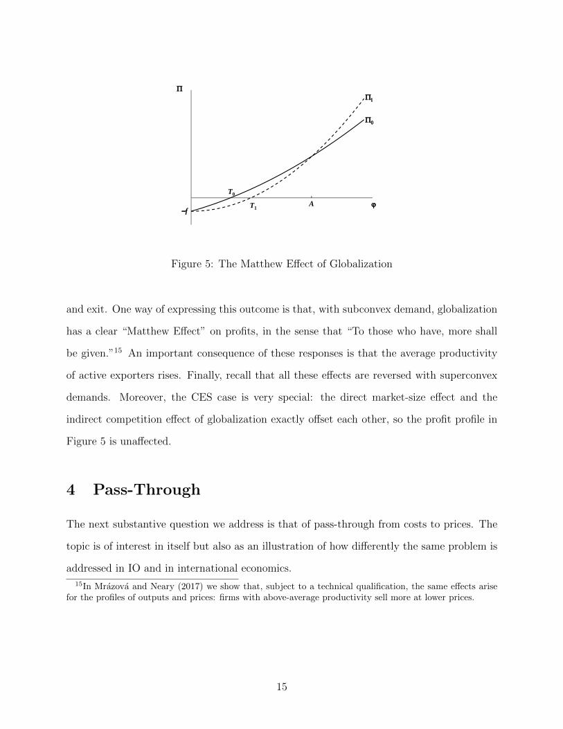
Figure 5 illustrates these effects in the case of subconvexity. The curve labelled Π0

shows the initial profit profile across firms of different productivity, while that labelled Π1

shows the profit profile after globalization, assuming that demand is strictly subconvex.

The productivity level denoted T0 is that corresponding to threshold firms in the initial

equilibrium: they make zero profits and so are indifferent between producing or not; while

that denoted A corresponds to the average firm that faces the demand elasticity ε. As can

be seen, in line with equation (12), the direct, market-expansion, effect dominates for firms

of above-average size, ε < ε, so they expand; the indirect, competition, effect dominates for

firms below average size, ε > ε, so they contract; and threshold firms cease to be profitable

14

T0

AT1f

Figure 5: The Matthew Effect of Globalization

and exit. One way of expressing this outcome is that, with subconvex demand, globalization

has a clear “Matthew Effect” on profits, in the sense that “To those who have, more shall

be given.”15 An important consequence of these responses is that the average productivity

of active exporters rises. Finally, recall that all these effects are reversed with superconvex

demands. Moreover, the CES case is very special: the direct market-size effect and the

indirect competition effect of globalization exactly offset each other, so the profit profile in

Figure 5 is unaffected.

4 Pass-Through

The next substantive question we address is that of pass-through from costs to prices. The

topic is of interest in itself but also as an illustration of how differently the same problem is

addressed in IO and in international economics.

15In Mrazova and Neary (2017) we show that, subject to a technical qualification, the same effects arisefor the profiles of outputs and prices: firms with above-average productivity sell more at lower prices.

15

4.1 Pass-Through in Industrial Organization

The archetypical pass-through question posed in industrial organization is both simple and

important: if marginal cost rises by a euro, by how much will a profit-maximizing firm

raise its price; i.e., how large is dp/dc? The answer is easy to calculate from the first-order

condition in (1):16

p+ xp′ = c ⇒ dp

dc=

1

2− ρ(13)

Thus a shock to costs is passed through to prices by more the more convex is the demand

function. Moreover, the threshold for full, or “euro-for-euro”, pass-through is that the degree

of convexity is exactly one:

dp

dc− 1 =

ρ− 1

2− ρ= 0 (14)

Demand functions implying constant pass-through are members of the Bulow-Pfleiderer

family, due to Bulow and Pfleiderer (1983):17

p(x) = β(x

1−κκ + γ

), β

1− κκ

< 0 (15)

This implies a constant pass-through coefficient equal to κ: dp/dc = κ. Special cases of

this include linear demand, with convexity ρ equal to zero and a constant pass-through of

κ = 1/2; and log-linear direct demand, p(x) = β′(log x + γ′), corresponding to a limiting

case of (15) with exactly one-for-one pass-through, κ = 1.18 The latter demand function

has convexity ρ equal to one, and so is the demand function implied by the condition in

(14) holding globally. In general, values of κ > 1 and ρ > 1 correspond to log-convex direct

demand, and values of κ < 1 and ρ < 1 to log-concave demand.

16This condition can be found in Cournot (1838), p. 79, which even allows for variable marginal cost. Seealso Bontems (2019).

17This demand function is more familiar when written, in the notation of Bulow and Pfleiderer, as p =α−βxδ, when δ 6= 0, and p = α−β log x. We write it differently to facilitate comparison with other demandfunctions to be introduced later.

18The limit has κ→ 1, β →∞, and γ → −1. To see this, set β = β′ κ1−κ and γ = γ′ 1−κκ − 1 and evaluate

the limit when κ→ 1, using for example a limited expansion.

16

4.2 Pass-Through in International Economics

Pass-through is also widely studied in international economics, both pass-through from tariffs

to domestic prices in international trade, and pass-through from exchange rates to domestic

prices in international monetary economics. However, the approach is totally different from

that in industrial organization: compare for example Gopinath and Itskhoki (2010) with

Weyl and Fabinger (2013), both important papers that refer to large literatures but have

only a single reference in common.19 It is not merely the answers that differ between the two

fields, but the questions too. In IO the focus is on absolute or euro-for-euro pass-through as

we have seen, whereas in international economics the question posed relates to proportional

pass-through: how large is d log p/d log c? Both approaches make perfect sense in their

respective contexts: IO scholars are typically analysing the effects of a cost or tax change on

a single industry, whereas in international economics the focus is on a change in policy or

exchange rates at the economy-wide level. The first question is a partial-equilibrium one, so

it is natural to work with absolute changes, whereas the second is a general-equilibrium one,

mandating a focus on relative prices and proportional changes. However, it is important to

understand the differences between the two.

Once again, the expression for proportional pass-through can be derived from the first-

order condition (1):

d log p

d log c=ε− 1

ε

1

2− ρ(16)

Unlike the corresponding term for absolute pass-through, (13), this depends on the elasticity

of demand as well as its convexity. So, the threshold for full (100%) proportional pass-

through is:

d log p

d log c− 1 =

ερ− ε− 1

2− ρ= 0 (17)

This is equivalent to the demand function taking the CES form, as we have already seen

that only in that case is the ratio p/c constant. (To show this explicitly, substitute for the

19The papers cite 41 and 86 references respectively, of which only Atkeson and Burstein (2008) is commonto both.

17

convexity of CES demand from (4) into (17).) This suggests that pass-through will be more

than 100% if and only if the demand function at the initial equilibrium is more convex than

a CES demand function. We will return to this below.

We saw in the previous sub-section that an important benchmark is the Bulow-Pfleiderer

demand family, which implies constant absolute pass-through. So it is natural to ask if there

are demand functions other than the CES that imply constant proportional pass-through

(CPPT): d log p/d log c = κ, κ 6= 1. The answer to this question is the CPPT family,

introduced in Mrazova and Neary (2017):20

p(x) =β

x

(x

κ−1κ + γ

) κκ−1

, β > 0, κ 6= 1 (18)

This family also has the property that it implies a constant proportional response of markups

to marginal costs: d log(p/c)/d log c = κ− 1.

4.3 Comparing Absolute and Proportional Pass-Through

Casual inspection suggests that the CPPT demand functions in (18) are very different from

the Bulow-Pfleiderer demands in equation (15). However, it is difficult to compare the two

directly: they have different functional forms with three parameters each. Instead, we use

the approach introduced in Section 2.2 of comparing the demand manifolds implied by the

demand functions. This also allows us to compare visually the conditions that imply constant

absolute and proportional pass-through.

By calculating the convexity of the Bulow-Pfleiderer demand function in equation (15),

we can show that the implied demand manifold is given by:

ρ(ε) = 2− 1

κ(19)

which is independent of ε. Similarly, by calculating both the elasticity and convexity of the

20The parameter γ must be strictly positive to ensure that the elasticity of demand exceeds one.

18

CPPT demand function in equation (18), the implied demand manifold is given by:

ρ(ε) = 2− 1

κ

ε− 1

ε(20)

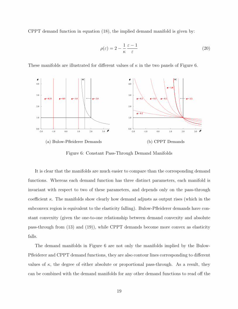
These manifolds are illustrated for different values of κ in the two panels of Figure 6.

0.0

1.0

2.0

3.0

4.0

-2.0 -1.0 0.0 1.0 2.0 3.0

SC

= 1.0 = 0.5 = 0.33 = 2.0

(a) Bulow-Pfleiderer Demands

0.0

1.0

2.0

3.0

4.0

-2.0 -1.0 0.0 1.0 2.0 3.0

= 0.5

= 0.1

= 0.3 = 0.2 = 2.5

= 1.0

SC

(b) CPPT Demands

Figure 6: Constant Pass-Through Demand Manifolds

It is clear that the manifolds are much easier to compare than the corresponding demand

functions. Whereas each demand function has three distinct parameters, each manifold is

invariant with respect to two of these parameters, and depends only on the pass-through

coefficient κ. The manifolds show clearly how demand adjusts as output rises (which in the

subconvex region is equivalent to the elasticity falling). Bulow-Pfleiderer demands have con-

stant convexity (given the one-to-one relationship between demand convexity and absolute

pass-through from (13) and (19)), while CPPT demands become more convex as elasticity

falls.

The demand manifolds in Figure 6 are not only the manifolds implied by the Bulow-

Pfleiderer and CPPT demand functions, they are also contour lines corresponding to different

values of κ, the degree of either absolute or proportional pass-through. As a result, they

can be combined with the demand manifolds for any other demand functions to read off the

19

rates of pass-through implied by those demands. For example, recalling the CARA, LES

and translog demand manifolds in Figure 2, we can see that all three imply a higher level of

absolute pass-through for large firms; LES demands imply a constant rate of proportional

pass-through for all firms, equal to 0.5, whereas CARA demands imply that the rate of

proportional pass-through decreases with firm size, and translog demands imply that it

increases.

5 Selection Effects

We turn next to one of the most distinctive and novel features of models with heterogeneous

firms: their ability to predict which firms will select into which activities. Consider first

the question of which firms will choose to export. Here the key prediction of the Melitz

(2003) model is that more productive firms select into exporting. It turns out that this is

an extremely robust result. It requires only that ex post profits π are decreasing in c, which

must be true in all models of this kind. To see this, write the maximized value of operating

profits as follows:

π(τ, c) ≡ maxx

π(x, τ, c), π(x, τ, c) = (p(x)− τc)x (21)

where τ is an iceberg trade cost: τ units must be produced and shipped to the export market

in order for one unit to arrive. For simplicity, assume that π(τ, c) is continuous in τ, c.

Differentiating (21) and invoking the envelope theorem, we can see that operating profits

are unambiguously decreasing in c:

πc = πc = −τx < 0 (22)

This result is independent of the form of the demand function; in particular, it is not sensitive

to whether demands are CES or not. Hence, ranking firms by their productivity, or inverse

20

marginal cost, unambiguously predicts their ranking by total profits, Π = π − f . So there

must be a unique threshold level of productivity, with all firms more productive than the

threshold choosing to export and all those less productive choosing not to.

1c1Ec 1

Fc

First-OrderSelection Effects

1Sc

Second-OrderSelection Effects

FDIExportsExit

E

F

fF

fE

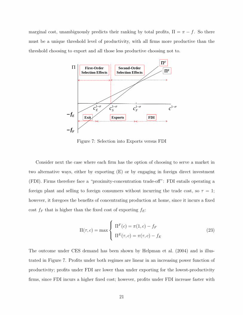
Figure 7: Selection into Exports versus FDI

Consider next the case where each firm has the option of choosing to serve a market in

two alternative ways, either by exporting (E) or by engaging in foreign direct investment

(FDI). Firms therefore face a “proximity-concentration trade-off”: FDI entails operating a

foreign plant and selling to foreign consumers without incurring the trade cost, so τ = 1;

however, it foregoes the benefits of concentrating production at home, since it incurs a fixed

cost fF that is higher than the fixed cost of exporting fE:

Π(τ, c) = max

ΠF (c) = π(1, c)− fF

ΠE(τ, c) = π(τ, c)− fE(23)

The outcome under CES demand has been shown by Helpman et al. (2004) and is illus-

trated in Figure 7. Profits under both regimes are linear in an increasing power function of

productivity; profits under FDI are lower than under exporting for the lowest-productivity

firms, since FDI incurs a higher fixed cost; however, profits under FDI increase faster with

21

productivity because FDI incurs lower access costs; and the two profit schedules intersect

only once as shown.21 As the lower set of labels indicates, there is now three-way selection,

with the least efficient firms not serving the market as before, firms of intermediate efficiency

exporting, and the most efficient firms engaging in FDI.

However, Mrazova and Neary (2019) show that this predicted selection pattern is less

robust than that for the choice between exporting or not. To see why, consider the upper

set of labels in Figure 7. These categorise productivity levels not in terms of their predicted

outcomes but in terms of the choices they offer to firms. Low-productivity firms, with costs

higher than cS (represented by points to the left of c1−σS in the figure), face the same choice

as before: FDI is not profitable, so the only decision they face is whether to export or not.

Mrazova and Neary (2019) call the outcomes of such a decision a “first-order selection effect”:

firms face a choice between one activity, exporting, whose profits vary with productivity, and

another, not exporting, whose profits are the same for all firms. This is in contrast to the

“second-order selection effect” that arise from the choices of high-productivity firms with

costs lower than cS. For such firms both exports and FDI are profitable, and their profitability

in both modes varies with productivity. Hence, the conventional sorting, where more efficient

firms select into FDI, is only guaranteed if the two curves have a single intersection as in

Figure 7. With a slight abuse of terminology we will refer to this configuration as the

single-crossing property.22

When might we expect the single-crossing property to hold? One consideration which

suggests that second-order selection effects may be less robust than first-order ones comes

from Appendix A. We show there that CES demands are the only case in which variable

profits are a power function of marginal cost, and so total profits are affine in a simple

21To ensure that both exports and FDI are observed we require that the two curves intersect in the positivequadrant, which is equivalent to the “freeness” of trade (the variable trade cost adjusted by the degree ofsubstitutability) being greater than the ratio of fixed costs: τ1−σ > fE/fF .

22In the language of monotone comparative statics, the condition for ΠE and ΠF to have only a singleintersection is that the function ΠF (c)−ΠE(τ, c) is single crossing from above. For details see Mrazova andNeary (2019). For further background on monotonic comparative statics, see Milgrom and Roberts (1990)and Vives (1990).

22

transformation of productivity as in Figure 7. Thus, with demands other than CES, we need

to establish whether the single-crossing property holds and so whether the second-order

selection effects will be as illustrated in Figure 7.

Checking directly whether the single-crossing property holds in any particular application

is not easy. However, it is easy to check for an important sufficient condition. Recall that π

is continuous in c, and assume also that the two profit functions ΠF and ΠE have different

slopes at any point where they intersect. Given this, the single-crossing property is equivalent

to ΠF being steeper than ΠE at any productivity level where they intersect, the configuration

shown in Figure 7. This suggests a sufficient condition for second-order selection effects which

is much easier to check: if ΠF is steeper than ΠE at every level of productivity, then single

crossing must hold. This condition is equivalent to πc(1, c) < πc(τ, c) at every value of c,

which, provided π is twice differentiable in (τ, c), is equivalent to a restriction on its second

derivative: πcτ is positive, or π(τ, c) is supermodular in (τ, c). A necessary and sufficient

condition for πcτ > 0 can be found in turn by differentiating (22) with respect to τ :

πcτ = −x− τ ∂x∂τ

= −x(

1 +d log x

d log c

)(24)

Hence π(τ, c) is supermodular in τ, c if and only if −d log x/d log c > 1; i.e., if and only if

the elasticity of output with respect to marginal cost is greater than one in absolute value.

(In what follows we denote this by “EMR” since it is also the elasticity of output with

respect to marginal revenue.) To understand this condition, note that supermodularity is a

restriction on a second derivative, that is, on a difference in differences: not whether higher

trade costs reduce profits, but whether they do so by less for lower-productivity firms. The

final term on the right-hand side of (24) shows that they are more likely to do so the more

elastic is the volume sold to an increase in costs. Offsetting this is the first term, equal to

one: this reflects the fact that higher trade costs reduce profits by less for a firm that is

selling less to begin with. Whether or not supermodularity obtains depends on the balance

23

between these two forces.

An alternative way of writing the condition for supermodularity in (24) allows us to

illustrate it in demand-manifold space. It can be expressed in terms of demand parameters

by noting that it equals the elasticity of demand times the elasticity of price with respect to

marginal cost, already given in (16) above:

−d log x

d log c= ε

d log p

d log c=ε− 1

2− ρ(25)

Supermodularity therefore requires that the following expression be positive:

−(

1 +d log x

d log c

)=ε+ ρ− 3

2− ρ(26)

Thus, from (24), selection into FDI by large firms is only guaranteed if the EMR is greater

than one in absolute value, which from (26) is equivalent to the demand function being

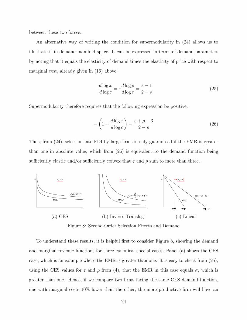
sufficiently elastic and/or sufficiently convex that ε and ρ sum to more than three.

p

x

MR(x)

0tc

/1)( xxp

(a) CES

0tc

(b) Inverse Translog

p

x

MR(x)

0tc

xxp )(

(c) Linear

Figure 8: Second-Order Selection Effects and Demand

To understand these results, it is helpful first to consider Figure 8, showing the demand

and marginal revenue functions for three canonical special cases. Panel (a) shows the CES

case, which is an example where the EMR is greater than one. It is easy to check from (25),

using the CES values for ε and ρ from (4), that the EMR in this case equals σ, which is

greater than one. Hence, if we compare two firms facing the same CES demand function,

one with marginal costs 10% lower than the other, the more productive firm will have an

24

output more than 10% higher than the less productive one. This helps explain the result of

Helpman et al. (2004), which exhibits another example of the Matthew Effect: in this case,

more efficient firms enjoy higher profits when they engage in FDI.

Panel (c), by contrast, shows the case of linear demands, which is an example where the

EMR is less than one for larger firms. Intuitively, for such large firms the additional trade

cost they must pay if they export is small, since their production cost is low to begin with,

and trade costs are proportional to production costs; moreover it reduces their sales very

little, since the marginal revenue curve is not steep. Hence, supermodularity fails for larger

firms under linear demands, and it can be shown that the largest ones will indeed exhibit

reverse selection effects, choosing to export rather than to engage in FDI.

Finally, Panel (b) shows a knife-edge case with the property that the EMR equals one.

As a result, the proximity-concentration trade-off yields the same outcome for all firms

irrespective of their productivity: the ΠX and ΠF curves in Figure 7 are parallel. Hence,

no firms will find it profitable to engage in FDI since it incurs a higher fixed cost, and so

no selection will be observed. Mrazova and Neary (2019) show that this demand function

is the inverse translog, p(x) = β′

x(log x + γ′). It is a limiting case of a family of demand

functions that exhibit a constant EMR: d log x/d log c = −κ. Mrazova et al. (2015) call this

the “CEMR” family:23

p(x) =β

x

(x

κ−1κ + γ

)β(κ− 1) > 0 (27)

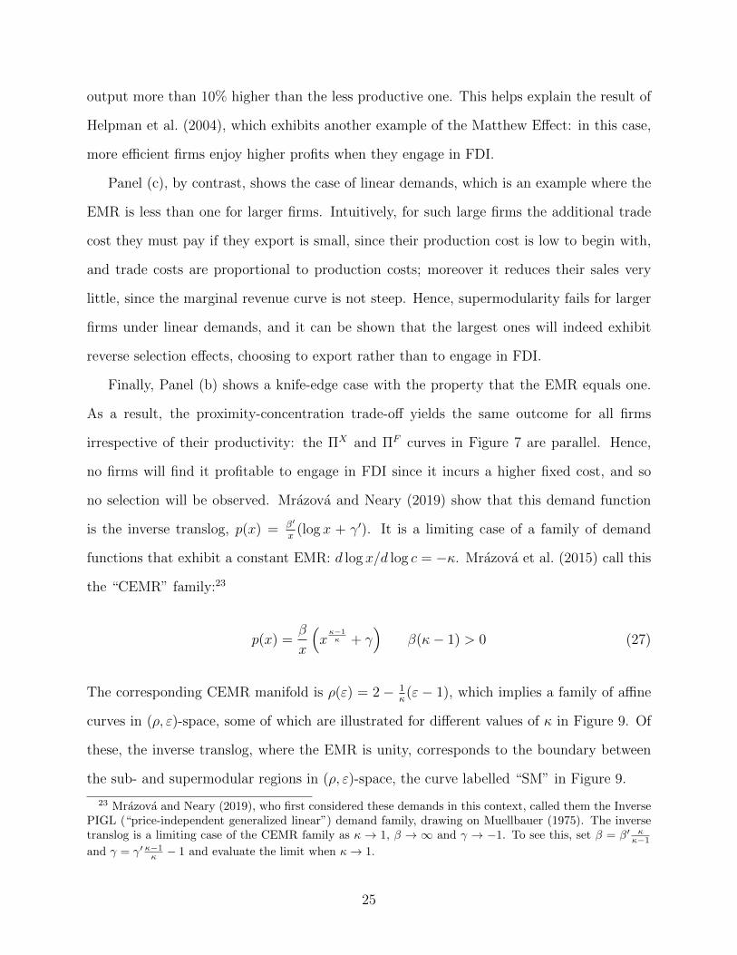
The corresponding CEMR manifold is ρ(ε) = 2− 1κ(ε− 1), which implies a family of affine

curves in (ρ, ε)-space, some of which are illustrated for different values of κ in Figure 9. Of

these, the inverse translog, where the EMR is unity, corresponds to the boundary between

the sub- and supermodular regions in (ρ, ε)-space, the curve labelled “SM” in Figure 9.

23 Mrazova and Neary (2019), who first considered these demands in this context, called them the InversePIGL (“price-independent generalized linear”) demand family, drawing on Muellbauer (1975). The inversetranslog is a limiting case of the CEMR family as κ → 1, β → ∞ and γ → −1. To see this, set β = β′ κ

κ−1and γ = γ′ κ−1κ − 1 and evaluate the limit when κ→ 1.

25

0.0

1.0

2.0

3.0

4.0

-2.0 -1.0 0.0 1.0 2.0 3.0

SM

SC

= 4 = 1 = 2

= 0.25

= 0.5

Figure 9: CEMR Demand Manifolds

6 Linking Productivity and Sales Distributions

The final substantive topic we want to discuss goes to the heart of firm heterogeneity in

models of monopolistic competition. It concerns the relationship between the shape of the

underlying distribution assumed for firm productivities, and the shape of the predicted dis-

tribution of firm outcomes, whether the level or the rate of growth of output or sales.24

There is a relatively small number of results of this kind. First is the canonical result in

the field, due to Helpman et al. (2004) and Chaney (2008): in the Melitz (2003) model of

heterogeneous firms, if firm productivities follow a Pareto distribution and demands are CES,

then firm sales must also follow a Pareto distribution. Second, going beyond the canonical

result, Head et al. (2014) retain the assumption that demands are CES, and show that if

firm productivities follow a Lognormal distribution instead of a Pareto then firm sales must

also follow a Lognormal distribution. This result is important as there is abundant evidence

that the distribution of firm sales is approximately Pareto for the “long tail” of large firms,

but is more closely approximated by a Lognormal distribution for the whole population of

firms, especially smaller ones: see, for example, Bee and Schiavo (2018).25

24This section draws on Mrazova et al. (2015).25Some authors have explored models of heterogeneous firms with other productivity distributions, includ-

ing generalizations or combinations of the Lognormal and Pareto such as mixtures of thin- and fat-tailed

26

Both these results share two features. First, they assume CES demands, and so imply

that all firms have the same markups which do not vary over time. Second, they exhibit a

property that Mrazova et al. (2015) call “self-reflection”: the distribution predicted for the

endogenous random variable takes the same form as, or “reflects,” the distribution assumed

for the exogenous random variable. Self-reflection is an attractive property: for example, it is

desirable to understand in what circumstances the analytically tractable Pareto distribution

can be used for both productivity and sales.26 Hence, it is desirable to know whether there

are demand functions other than the CES that are consistent with this property.

Mrazova et al. (2015) show that the answer to this question is “yes” by deriving conditions

for self-reflection of two distributions, where the firm-level variables are linked by a functional

relationship. They introduce a class of distributions, the “Generalized Power Function”

(GPF) class, that nests many well-known families of distributions, including the Pareto,

Lognormal and Frechet. They then show that, if the distributions of both variables are

members of the same family in this class, it then follows that the relationship between

the two variables must take a simple power-law form. Moreover, these three conditions

are necessary and sufficient for each other in the sense that any two imply the third. In

the present context, the variables of interest are productivity and sales revenue, so the

requirement for self-reflection is that sales revenue is a power-law function of productivity.

Since productivity is the inverse of marginal cost, this is equivalent to a constant elasticity

of sales revenue with respect to marginal cost: d log r/d log c = −κ. Of course, marginal

cost equals marginal revenue in equilibrium, so this condition can also be expressed as a

“Constant Revenue Elasticity of Marginal Revenue,” whence the acronym “CREMR”.

The next step is to derive the demand functions that exhibit the CREMR property. It is

straightforward to express the elasticity in terms of ε and ρ, using the fact that r(x) = xp(x)

Pareto or piecewise Lognormal-Pareto distributions, although these are typically not analytically tractable.See, for example, Luttmer (2007), Eaton et al. (2011), Edmonds et al. (2012), and Nigai (2017).

26Mrazova et al. (2015) show that self-reflection is also necessary and sufficient for models of monopolisticcompetition to exhibit Gibrat’s Law, the classic result due to Gibrat (1931) that a firm’s rate of growthshould be independent of its size.

27

and the expression for the elasticity of output with respect to marginal cost from (25):

d log r

d log c=ε− 1

ε

d log x

d log c= − (ε− 1)2

ε(2− ρ)(28)

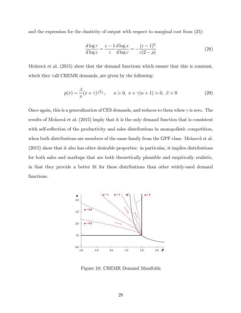
Mrazova et al. (2015) show that the demand functions which ensure that this is constant,

which they call CREMR demands, are given by the following:

p(x) =β

x(x+ γ)

κκ+1 , κ > 0, x+ γ(κ+ 1) > 0, β > 0 (29)

Once again, this is a generalization of CES demands, and reduces to them when γ is zero. The

results of Mrazova et al. (2015) imply that it is the only demand function that is consistent

with self-reflection of the productivity and sales distributions in monopolistic competition,

when both distributions are members of the same family from the GPF class. Mrazova et al.

(2015) show that it also has other desirable properties: in particular, it implies distributions

for both sales and markups that are both theoretically plausible and empirically realistic,

in that they provide a better fit for these distributions than other widely-used demand

functions.

0.0

1.0

2.0

3.0

4.0

-2.0 -1.0 0.0 1.0 2.0 3.0

= 0.2

= 0.5

= 1 = 5 = 2 SC

Figure 10: CREMR Demand Manifolds

28

Finally, we can calculate the CREMR demand manifold, which is given by the following:

ρ(ε) = 2− 1

κ

(ε− 1)2

ε(30)

Figure 10 illustrates some examples of this for different values of κ. Once again, these

are very different from the demand manifolds for standard demand functions, as shown in

Figure 2.

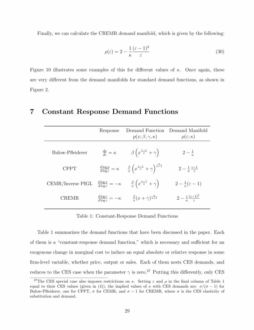
7 Constant Response Demand Functions

Response Demand Function Demand Manifoldp(x; β, γ, κ) ρ(ε;κ)

Bulow-Pfleiderer dpdc

= κ β(x

1−κκ + γ

)2− 1

κ

CPPT d log pd log c

= κ βx

(x

κ−1κ + γ

) κκ−1

2− 1κε−1ε

CEMR/Inverse PIGL d log xd log c

= −κ βx

(x

κ−1κ + γ

)2− 1

κ(ε− 1)

CREMR d log rd log c

= −κ βx(x+ γ)

κκ+1 2− 1

κ(ε−1)2

ε

Table 1: Constant-Response Demand Functions

Table 1 summarizes the demand functions that have been discussed in the paper. Each

of them is a “constant-response demand function,” which is necessary and sufficient for an

exogenous change in marginal cost to induce an equal absolute or relative response in some

firm-level variable, whether price, output or sales. Each of them nests CES demands, and

reduces to the CES case when the parameter γ is zero.27 Putting this differently, only CES

27The CES special case also imposes restrictions on κ. Setting ε and ρ in the final column of Table 1equal to their CES values (given in (4)), the implied values of κ with CES demands are: σ/(σ − 1) forBulow-Pfleiderer, one for CPPT, σ for CEMR, and σ − 1 for CREMR, where σ is the CES elasticity ofsubstitution and demand.

29

demands imply constant responses to costs of more than one of these variables, and each of

the four demand functions in Table 1 allows for variable markups if and only if γ is non-zero.

The explicit expressions for the different demand functions given in the third column

of the table are suggestive. Yet even though they are written in ways that makes them as

comparable as possible, their behavior relative to each other is not immediately obvious. It

is easier to compare their properties using their manifolds, as shown in the fourth column,

and as illustrated in Figures 6, 9, and 10. While each demand function depends on three

parameters, each of the manifolds depends only on κ, the parameter that measures the

response of the variable in question to the change in marginal cost. Thus, as we have seen in

previous sections, each manifold is a locus of values of ε and ρ which ensure that the relevant

response to an increase in marginal cost is constant.

Except for the Bulow-Pfleiderer case, the other three demand functions in Table 1 have

manifolds that are mostly quite different from those of the better-known and more widely-

used demand functions shown in Figure 2. If we concentrate on the subconvex case, we

can see that these demand functions allow for much more concavity than most widely-used

demands. This is especially true for firms that are small and relatively unresponsive to

shocks (i.e., for high values of ε and low values of κ). Mrazova et al. (2015) point out that

this ability to allow small firms to face very concave demand may be why CREMR demands

give a better fit to both sales and markups than other demand systems. By contrast, for

larger firms (i.e., for lower values of ε), Bulow-Pfleiderer demands have constant convexity by

construction, whereas the others become steadily more convex: CPPT and CEMR asymptote

to Cobb-Douglas, and CREMR to a general CES with elasticity of demand σ equal to κ+ 1.

While the manifolds in Table 1 are invariant with respect to the other two demand

parameters β and γ, this does not imply that these have no role. Consider first the non-

CES parameter γ: its sign is a key determinant of whether a given demand function is

sub- or superconvex. More specifically, if, for a given value of κ, a demand function can be

either sub- or superconvex, then it is superconvex if and only if γ is positive. Table 3 in

30

Appendix C illustrates the possible configurations in detail. As for the parameter β, its role

in these demand functions is similar to the one it plays in the CES itself: it affects only the

level of demand, and is taken as given by firms, but is determined endogenously in general

equilibrium. We saw in Section 3 how this gives rise to competition effects. In general, any

exogenous shock to an industry equilibrium will have both a direct effect on individual firms

and an indirect competition effect working through the free entry condition and the demand

function. As we saw in Section 3, the competition effect operates in a particularly simple

way when demand is generated by additively separable preferences, since it affects only β,

which is inversely proportional to the marginal utility of income. Finally, a further role

played by the β parameter arises if we want to move from demands to preferences. All of the

demand functions in Table 1 can be integrated to get the corresponding preference system,

which allows us to solve for the endogenous value of β. This is relatively straightforward

when cross-price effects take a simple form, as in the case of additive separability or Kimball

preferences. (Mrazova et al. (2015) discuss this further for CREMR demands.) Hence, these

demand functions can be used in explicit calculations of the general-equilibrium welfare

effects of policy and other shocks.

Finally, in both theoretical and empirical applications it may be convenient to work with

demand functions that nest some or all of the families in Table 1. By introducing just one

extra parameter we can write a generalized constant-response demand function that nests

the CPPT, CEMR and CREMR cases.28 This takes the following form:

p(x) =β

x(xα + γ)θ (31)

It is obvious by inspection that this nests the CPPT, CEMR and CREMR demand functions.

Moreover, we can check that it implies a constant proportional response to a change in

28We can introduce yet one further parameter to write a generalized demand function that nests allfour cases in Table 1. However, whereas the constant response implied by Bulow-Pfleiderer demands is anabsolute one, we focus here on nesting the three demand functions (CPPT, CEMR and CREMR) that implya constant proportional response to costs of a variable that we can also nest by a general constant responsefunction implied by (31).

31

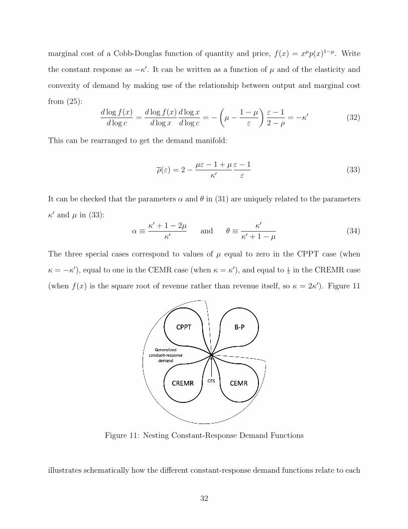
marginal cost of a Cobb-Douglas function of quantity and price, f(x) = xµp(x)1−µ. Write

the constant response as −κ′. It can be written as a function of µ and of the elasticity and

convexity of demand by making use of the relationship between output and marginal cost

from (25):

d log f(x)

d log c=d log f(x)

d log x

d log x

d log c= −

(µ− 1− µ

ε

)ε− 1

2− ρ= −κ′ (32)

This can be rearranged to get the demand manifold:

ρ(ε) = 2− µε− 1 + µ

κ′ε− 1

ε(33)

It can be checked that the parameters α and θ in (31) are uniquely related to the parameters

κ′ and µ in (33):

α ≡ κ′ + 1− 2µ

κ′and θ ≡ κ′

κ′ + 1− µ(34)

The three special cases correspond to values of µ equal to zero in the CPPT case (when

κ = −κ′), equal to one in the CEMR case (when κ = κ′), and equal to 12 in the CREMR case

(when f(x) is the square root of revenue rather than revenue itself, so κ = 2κ′). Figure 11

Figure 11: Nesting Constant-Response Demand Functions

illustrates schematically how the different constant-response demand functions relate to each

32

other: all except Bulow-Pfleiderer demands are nested by (31), and the CES is the only

demand function that is nested by all.29

8 Conclusion

In this paper we have reviewed and extended recent work by ourselves and others on mo-

nopolistic competition in benchmark models of international trade.30 We have concentrated

on the implications of such models for a number of important results, including competi-

tion effects, pass-through, selection effects, and the size distribution of firms. One unifying

principle we have emphasized is that the assumption of CES preferences and demands yields

enormous analytical tractability, but also has very restrictive and often counter-factual impli-

cations. In a CES world, competition effects take a very simple form: all firms have the same

markup, and globalization shocks leave the distribution of profits across firms unchanged;

pass-through from costs to prices is always exactly 100%; larger firms always select into

activities with lower access costs; and the distributions of productivity and sales typically

exhibit the same form. A second unifying principle that we have highlighted is the class

of constant-response demand functions that provide a parsimonious suite of alternatives to

the CES case. Each of these functions adds a single parameter to the CES, so avoiding the

counter-factual prediction of constant markups, while preserving one or other of its key prop-

erties. Given the dominance of monopolistic competition in trade, these demand functions

provide a route to more realistic modelling and empirical work. Moreover, the generalized

constant-response demand function that we introduced in Section 7 will hopefully prove

helpful in giving a unified perspective on the different individual constant-response functions

and in understanding how they relate to each other.

29Matsuyama and Ushchev (2017) illustrate in a similar way links between non-parametric homotheticdepartures from CES.

30As already mentioned, we have not discussed trade under oligopoly, which provides an alternative expla-nation for the evidence of variable markups cited in Section 2.3. (See, for example, Neary (2003, 2016) andAtkeson and Burstein (2008).) Nor have we discussed the extensive recent literature in trade that uses cali-bration methods to quantify the effects of exogenous shocks, often in CES-based frameworks. (See Costinotand Rodrıguez-Clare (2014) for an overview.)

33

The fact that the monopolistically competitive paradigm has become the dominant one

in international trade may seem surprising from an IO perspective. However, there are good

reasons for this. The availability of large data sets on exporting firms, and the desire to take

account of general-equilibrium feedbacks between goods and factor markets, make a “one-

size-fits-all” approach to the choice of market structure very convenient. This is despite the

fact that it is sure to miss much of the supply-side specificity on which IO economists tend

to focus, including industry-specific features such as limit pricing in some industries but not

in others, differences in fixed costs, the role of learning-by-doing, etc. Moreover, as we have

shown, relaxing the assumption of CES preferences in monopolistic competition makes its

view of firms more realistic and its predictions more flexible.

Of course, while leaving the comfort zone of CES goes part of the way to a more realistic

view of imperfectly competitive markets, it raises new problems. To paraphrase Tolstoy

(1878), CES demand functions are all alike, every non-CES demand function is non-CES in

its own way.31 The CES benchmark is sure to retain a central place in this field, both because

of its tractability and also because it alone exhibits all the constant-response properties that

we have discussed.

In conclusion, we have already noted some ironies in the selective way in which inter-

national trade has borrowed from industrial organization in how it models firms in open

economies. In particular, Dixit and Stiglitz proposed using additively separable preferences

as a way of modelling product differentiation, and viewed CES preferences as just a special

illustrative case; whereas it is the latter that has become the workhorse model for exploring

a huge range of issues in trade. There is a further irony. The substantive issue Dixit and

Stiglitz addressed was the efficiency of the market equilibrium, and in particular whether

an unregulated monopolistically competitive market would lead to too many or too few va-

rieties, and to firms that are too large or too small relative to the social optimum. This

issue has not been addressed much in trade, but in recent years there has been a revival of

31From the opening sentence of Anna Karenina: “Happy families are all alike; every unhappy family isunhappy in its own way.”

34

interest in it: see for example Feenstra and Kee (2008) and Dhingra and Morrow (2019). In

ongoing work with Mathieu Parenti (see Mrazova et al. (2015)) we show how the tools from

Section 6 above can be used to throw light on this issue.

Appendices

A Constant Response of Profits Demand Functions

We would like to characterize the demand functions with the property that operating profits

have a constant proportional response to marginal cost: d log πd log c

= κ. We know that this holds

in the CES case, where π = Bc1−σ.32 To find the necessary condition for this property, note

that, since π = (p− c)x, we have in general:

d log π = d log (p− c) + d log x (35)

Equation (25) gives the proportional response of output to changes in marginal cost, d log x/d log c.

The next step is to consider d log (p− c). Consider first d (p− c). From the firm’s first-order

condition this equals d (−xp′) = −p′dx− xp′′dx = − (p′ + xp′′) dx. Hence:

d log (p− c) =d (−xp′)−xp′

=(p′ + xp′′) dx

xp′=p′ + xp′′

p′d log x = (1− ρ) d log x (36)

Collecting terms gives, from (25) and (35):

d log π

d log c=d log (p− c)d log c

+d log x

d log c= (2− ρ)

d log x

d log c= − (ε− 1) (37)

32Here B is exogenous from the firm’s perspective, but it depends on the price index and on aggregateincome, and so is endogenous in general equilibrium. See, for example, Melitz (2003), equation (4).

35

Clearly the CES case is the only one that yields a constant value of this. Hence CES de-

mands are necessary and sufficient for a constant proportional response of operating profits

to marginal cost. This in turn implies that there is no other demand function which guar-

antees that profits are affine in a power-law transformation of costs, so we must seek other

conditions, such as supermodularity of the profit function in production and trade costs, to

be sure that second-order selection effects follow the same pattern as they do in the CES

case.

B Manifolds for Some Common Demand Functions

Demand Function Demand Manifold

CARA x(p) = γ + δ log p ρ(ε) = 1ε

Stone-Geary/LES p(x) = βγx+1

ρ(ε) = 2ε

Translog/AI x(p) = 1p

(γ + δ log p) ρ(ε) = 3ε−1ε2

Table 2: Some Common Demand Functions and Their Manifolds

Table 2 gives some common demand functions and their manifolds, as illustrated in Figure 2.

Further details are given in Mrazova and Neary (2017). As elsewhere in the paper, the

demand functions are written from the perspective of an individual firm in monopolistic

competition. They also depend on aggregate expenditure and on indices of the prices of

all goods, including the good in question; these are taken as given by the firm, since it is

of measure zero, and are subsumed into the demand parameters. (See Dixit and Stiglitz

(1993) for further discussion.) All three manifolds are invariant with respect to these other

variables. To take a specific example, Stone-Geary demands are more familiar when written

as: x(i) = α(i) + (p(i))−1(I −

∫i′∈Ω

p(i′)α(i′)di′), which, when γ = (−α(i))−1 and β =

36

γ(I −

∫p(i′)α(i′)di′

), is equivalent to the expression in Table 2. The latter expression is the

special case of the CPPT demands from (18) when κ = 1/2.

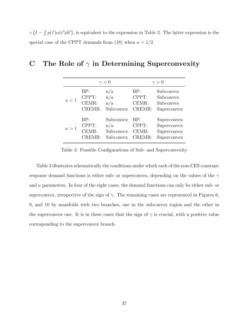
C The Role of γ in Determining Superconvexity

γ < 0 γ > 0

κ < 1

BP: n/a BP: SubconvexCPPT: n/a CPPT: SubconvexCEMR: n/a CEMR: SubconvexCREMR: Subconvex CREMR: Superconvex

κ > 1

BP: Subconvex BP: SuperconvexCPPT: n/a CPPT: SuperconvexCEMR: Subconvex CEMR: SuperconvexCREMR: Subconvex CREMR: Superconvex

Table 3: Possible Configurations of Sub- and Superconvexity

Table 3 illustrates schematically the conditions under which each of the non-CES constant-

response demand functions is either sub- or superconvex, depending on the values of the γ

and κ parameters. In four of the eight cases, the demand functions can only be either sub- or

superconvex, irrespective of the sign of γ. The remaining cases are represented in Figures 6,

9, and 10 by manifolds with two branches, one in the subconvex region and the other in

the superconvex one. It is in these cases that the sign of γ is crucial, with a positive value

corresponding to the superconvex branch.

37

References

Anderson, S. P., A. De Palma, and J.-F. Thisse (1992): Discrete Choice Theory of

Product Differentiation, Cambridge, MA: MIT Press.

Arkolakis, C. (2010): “Market Penetration Costs and the New Consumers Margin in

International Trade: Appendix,” web appendix, Yale University.

——— (2016): “A Unified Theory of Firm Selection and Growth,” Quarterly Journal of

Economics, 131, 89–155.

Atkeson, A. and A. Burstein (2008): “Pricing-to-Market, Trade Costs, and Interna-

tional Relative Prices,” American Economic Review, 98, 1998–2031.

Bache, P. A. and A. Laugesen (2015): “Monotone Comparative Statics for the Industry

Composition,” Working Paper, Aarhus University.

Bee, M. and S. Schiavo (2018): “Powerless: Gains from Trade when Firm Productivity

is not Pareto Distributed,” Review of World Economics, 154, 15–45.

Behrens, K. and Y. Murata (2007): “General Equilibrium Models of Monopolistic

Competition: A New Approach,” Journal of Economic Theory, 136, 776–787.

Bertoletti, P. and P. Epifani (2014): “Monopolistic Competition: CES Redux?” Jour-

nal of International Economics, 93, 227–238.

Bontems, P. (2019): “Not Too Costly: How Cost Flexibility Influences Firm Behavior,”

presented to ETSG 2019, Bern, Switzerland.

Brander, J. A. (1995): “Strategic Trade Policy,” in G.M. Grossman and K. Rogoff (eds.):

Handbook of International Economics, Volume 3, Amsterdam: Elsevier.

Bulow, J. I. and P. Pfleiderer (1983): “A Note on the Effect of Cost Changes on

Prices,” Journal of Political Economy, 91, 182–185.

38

Cabral, L. M. (2018): “Standing on the Shoulders of Dwarfs: Dominant Firms and Inno-

vation Incentives,” CEPR Discussion Paper No. 13115.

Chamberlin, E. H. (1933): The Theory of Monopolistic Competition: A Re-Orientation

of the Theory of Value, Cambridge, Mass: Harvard University Press.

Chaney, T. (2008): “Distorted Gravity: The Intensive and Extensive Margins of Interna-

tional Trade,” American Economic Review, 98, 1707–1721.

Costinot, A. and A. Rodrıguez-Clare (2014): “Trade Theory with Numbers: Quan-

tifying the Consequences of Globalization,” in G. Gopinath, E. Helpman and K. Rogoff

(eds.): Handbook of International Economics, Elsevier, 197–261.

Cournot, A. (1838): Recherches Sur les Principes Mathematiques de la Theorie des

Richesses, Paris: Gratiot.

De Loecker, J., P. K. Goldberg, A. K. Khandelwal, and N. Pavcnik (2016):

“Prices, Markups and Trade Reform,” Econometrica, 84, 445–510.

Deaton, A. and J. Muellbauer (1980): “An Almost Ideal Demand System,” American

Economic Review, 70, 312–326.

Dhingra, S. and J. Morrow (2019): “Monopolistic Competition and Optimum Product

Diversity under Firm Heterogeneity,” Journal of Political Economy, 127, 196–232.

Dixit, A. and V. Norman (1980): Theory of International Trade, Cambridge University

Press.

Dixit, A. K. (2004): “Some Reflections on Theories and Applications of Monopolistic Com-

petition,” in S. Brakman and B.J. Heijdra (eds): The Monopolistic Competition Revolution

in Retrospect, Cambridge: Cambridge University Press, 123-133.

Dixit, A. K. and J. E. Stiglitz (1977): “Monopolistic Competition and Optimum

Product Diversity,” American Economic Review, 67, 297–308.

39

——— (1993): “Monopolistic Competition and Optimum Product Diversity: Reply [to Yang

and Heijdra],” American Economic Review, 83, 302–304.

Eaton, J., S. Kortum, and F. Kramarz (2011): “An Anatomy of International Trade:

Evidence from French Firms,” Econometrica, 79, 1453–1498.

Eckel, C., L. Iacovone, B. Javorcik, and J. P. Neary (2015): “Multi-Product Firms

at Home and Away: Cost- versus Quality-Based Competence,” Journal of International

Economics, 95, 216–232.

Eckel, C. and J. P. Neary (2010): “Multi-Product Firms and Flexible Manufacturing

in the Global Economy,” Review of Economic Studies, 77, 188–217.

Feenstra, R. and H. L. Kee (2008): “Export Variety and Country Productivity: Esti-

mating the Monopolistic Competition Model with Endogenous Productivity,” Journal of

International Economics, 74, 500–518.

Feenstra, R. C. and D. E. Weinstein (2017): “Globalization, Markups, and U.S.

Welfare,” Journal of Political Economy, 125, 1040–1074.

Gaubert, C. and O. Itskhoki (2018): “Granular Comparative Advantage,” mimeo.,

University of California at Berkeley.

Gibrat, R. (1931): Les inegalites economiques: applications d’une loi nouvelle, la loi de

l’effet proportionnel [Economic Inequalities: Applications of a New Law, the Law of Pro-

portionate Effect], Librairie du Recueil Sirey.

Gopinath, G. and O. Itskhoki (2010): “Frequency of price adjustment and pass-

through,” Quarterly Journal of Economics, 125, 675–727.

Head, K., T. Mayer, and M. Thoenig (2014): “Welfare and Trade Without Pareto,”

American Economic Review, Papers and Proceedings, 104, 310–316.

40

Helpman, E., M. J. Melitz, and S. R. Yeaple (2004): “Export Versus FDI with

Heterogeneous Firms,” American Economic Review, 94, 300–316.

Krugman, P. (1980): “Scale Economies, Product Differentiation, and the Pattern of

Trade,” American Economic Review, 70, 950–959.

Krugman, P. R. (1979): “Increasing Returns, Monopolistic Competition, and Interna-

tional Trade,” Journal of International Economics, 9, 469–479.

Kuhn, K.-U. and X. Vives (1999): “Excess Entry, Vertical Integration, and Welfare,”

RAND Journal of Economics, 30, 575–603.

Lamorgese, A., A. Linarello, and F. Warzynski (2014): “Free Trade Agreements

and Firm-Product Markups in Chilean Manufacturing,” Tech. rep., Aarhus University.

Luttmer, E. G. (2007): “Selection, Growth, and the Size Distribution of Firms,” Quarterly

Journal of Economics, 122, 1103–1144.

Marshall, A. (1920): Principles of Economics, An Introductory Volume, Eighth Edition,

London: Macmillan.

Matsuyama, K. and P. Ushchev (2017): “Beyond CES: Three Alternative Classes of

Flexible Homothetic Demand Systems,” HSE Working Paper BRP 172/EC/2017, National

Research University Higher School of Economics.

Melitz, M. J. (2003): “The Impact of Trade on Intra-Industry Reallocations and Aggregate

Industry Productivity,” Econometrica, 71, 1695–1725.

Melitz, M. J. and G. I. Ottaviano (2008): “Market Size, Trade, and Productivity,”

Review of Economic Studies, 75, 295–316.

Milgrom, P. and J. Roberts (1990): “The Economics of Modern Manufacturing: Tech-

nology, Strategy, and Organization,” American Economic Review, 80, 511–528.

41

Mrazova, M. (2011): “Trade Agreements when Profits Matter,” Discussion Paper, De-

partment of Economics, University of Surrey.

Mrazova, M. and J. P. Neary (2014): “Together at Last: Trade Costs, Demand Struc-

ture, and Welfare,” American Economic Review, Papers and Proceedings, 104, 298–303.

Mrazova, M. and J. P. Neary (2017): “Not So Demanding: Demand Structure and

Firm Behavior,” American Economic Review, 107, 3835–3874.

——— (2019): “Selection Effects with Heterogeneous Firms,” Journal of the European Eco-

nomic Association, 17, 1294–1334.

Mrazova, M., J. P. Neary, and M. Parenti (2015): “Sales and Markup Dispersion:

Theory and Empirics,” revised June 2019.

Mrazova, M., D. Vines, and B. Zissimos (2013): “Is the GATT/WTO’s Article XXIV

bad?” Journal of International Economics, 89, 216–232.

Muellbauer, J. (1975): “Aggregation, Income Distribution and Consumer Demand,” Re-

view of Economic Studies, 42, 525–543.

Neary, J. P. (2003a): “Globalization and Market Structure,” Journal of the European

Economic Association, 1, 245–271.

——— (2003b): “Monopolistic Competition and International Trade Theory,” in S. Brak-

man and B.J. Heijdra (eds.): The Monopolistic Competition Revolution in Retrospect,

Cambridge University Press, 159-184.

——— (2007): “Cross-Border Mergers as Instruments of Comparative Advantage,” Review

of Economic Studies, 74, 1229–1257.

——— (2010): “Two and a Half Theories of Trade,” The World Economy, 33, 1–19.

42

——— (2016): “International Trade in General Oligopolistic Equilibrium,” Review of Inter-

national Economics, 24, 669–698.

Nigai, S. (2017): “A Tale of Two Tails: Productivity Distribution and the Gains from

Trade,” Journal of International Economics, 104, 44–62.

Nocke, V. and N. Schutz (2018): “Oligopoly in International Trade: An Aggregative

Games Approach,” presented to EARIE 2018, Athens.

Parenti, M. (2018): “Large and Small Firms in a Global Market: David vs. Goliath,”

Journal of International Economics, 110, 103–118.

Parenti, M., P. Ushchev, and J.-F. Thisse (2017): “Toward a Theory of Monopolistic

Ccompetition,” Journal of Economic Theory, 167, 86–115.

Pascoa, M. R. (1993): “Noncooperative Equilibrium and Chamberlinian Monopolistic

Competition,” Journal of Economic Theory, 60, 335–353.

——— (1997): “Monopolistic Competition and Non-Neighboring Goods,” Economic Theory,

9, 129–142.

Pollak, R. A. (1972): “Generalized Separability,” Econometrica, 40, 431–453.

Shimomura, K.-I. and J.-F. Thisse (2012): “Competition Among the Big and the

Small,” RAND Journal of Economics, 43, 329–347.

Simonovska, I. (2015): “Income Differences and Prices of Tradables: Insights from an

Online Retailer,” Review of Economic Studies, 82, 1612–1656.

Stiglitz, J. E. (2004): “Reflections on the State of the Theory of Monopolistic Compe-

tition,” in S. Brakman and B.J. Heijdra (eds): The Monopolistic Competition Revolution

in Retrospect, Cambridge: Cambridge University Press, 134-148.

43

Tolstoy, L. (1878): Anna Karenina, translated by Rosemary Edmonds, Harmondsworth,

Middlesex: Penguin Classics, 1954.

Vives, X. (1990): “Nash Equilibrium with Strategic Complementarities,” Journal of Math-

ematical Economics, 19, 305–321.

——— (1999): Oligopoly Pricing: Old Ideas and New Tools, Cambridge, Mass.: MIT Press.

Weyl, E. G. and M. Fabinger (2013): “Pass-Through as an Economic Tool: Principles

of Incidence under Imperfect Competition,” Journal of Political Economy, 121, 528–583.

Zhelobodko, E., S. Kokovin, M. Parenti, and J.-F. Thisse (2012): “Monopolistic

Competition: Beyond the Constant Elasticity of Substitution,” Econometrica, 80, 2765–

2784.

44