Investigation of tropospheric arcticaerosol and mixed-phase clouds using

airborne lidar technique

Dissertation

zur Erlangung des akademischen GradesDoktor der Naturwissenschaften (Dr. rer. nat.)

in der Wissenschaftsdisziplin Physik der Atmosphare

eingereicht an derMathematisch-Naturwissenschaftlichen Fakultat

der Universitat Potsdam

vonIwona Sylwia Stachlewska

Stiftung Alfred-Wegener-Institut fur Polar- und MeeresforschungForschungsstelle Potsdam, Telegrafenberg 43A, 14473 Potsdam

Potsdam, November 2005

I dedicate this piece of work to my beloved parents and siblings...My mother, Teresa, who taught me to fence through my life, win, lose but never

give up. My father, Henryk, who taught me a hard brave work as a way to exceedlimits of impossible. My sisters, Ola, Gosia and Agata, and brothers, Piotr, Micha�land Arek, who taught me that self-realisation comes through sharing and giving.

Contents

1 Introduction 31.1 Importance of aerosols and clouds . . . . . . . . . . . . . . . . . . . . . . . 31.2 Aerosols and clouds in the Arctic . . . . . . . . . . . . . . . . . . . . . . . . 51.3 Measurement techniques of aerosols and clouds . . . . . . . . . . . . . . . . 7

1.3.1 Lidar as a vital tool for atmospheric studies . . . . . . . . . . . . . . 81.3.2 Optical and microphysical parameter retrieval from lidar signals . . 8

2 Arctic field campaigns 102.1 Scientific activities during ASTAR 2004 . . . . . . . . . . . . . . . . . . . . 11

2.1.1 Airborne activities . . . . . . . . . . . . . . . . . . . . . . . . . . . . 122.1.2 Ground based, satellite and modelling activities . . . . . . . . . . . . 15

2.2 Scientific activities during SVALEX 2005 . . . . . . . . . . . . . . . . . . . 19

3 AWI lidars for measurements during Arctic field campaigns 203.1 The stationary Koldewey Aerosol Raman Lidar KARL . . . . . . . . . . . . 203.2 The new Airborne Mobile Aerosol Lidar AMALi . . . . . . . . . . . . . . . 20

3.2.1 Optical assembly . . . . . . . . . . . . . . . . . . . . . . . . . . . . . 213.2.2 Transmitting system . . . . . . . . . . . . . . . . . . . . . . . . . . . 223.2.3 Receiving and detecting system . . . . . . . . . . . . . . . . . . . . . 233.2.4 Data acquisition system . . . . . . . . . . . . . . . . . . . . . . . . . 243.2.5 AMALi end-products and their applications . . . . . . . . . . . . . . 25

4 Data evaluation schemes and error sources discussion 274.1 Backscatter lidar techniques . . . . . . . . . . . . . . . . . . . . . . . . . . . 284.2 Backscatter lidar equation . . . . . . . . . . . . . . . . . . . . . . . . . . . . 294.3 Diverse approaches for the elastic backscatter lidar retrieval . . . . . . . . . 30

4.3.1 Solution for an aerosol rich homogeneous atmosphere (slope methodapproach) . . . . . . . . . . . . . . . . . . . . . . . . . . . . . . . . . 30

4.3.2 Solution for aerosol rich heterogenious atmosphere (Klett approach) 314.3.3 Solution for a heterogenious atmosphere with aerosol rich and aerosol

free layers (Klett-Fernald approach) . . . . . . . . . . . . . . . . . . 314.4 Ansmann approach for inelestic backscatter lidar retrieval . . . . . . . . . . 334.5 Two-stream approach for elastic backscatter lidar retrieval and estimation

of lidar instrumental constants . . . . . . . . . . . . . . . . . . . . . . . . . 344.5.1 Retrieval of extinction, backscatter and lidar ratio profiles . . . . . . 344.5.2 Estimation of lidar instrumental constants . . . . . . . . . . . . . . . 36

4.6 Iterative Klett approach for airborne elastic backscatter lidar retrieval . . . 374.7 Direct retrieval of aerosol microphysical parameters . . . . . . . . . . . . . . 38

5 Lidar data analysis and applications 395.1 Meteorological situation during the ASTAR 2004 and SVALEX 2005 cam-

paigns . . . . . . . . . . . . . . . . . . . . . . . . . . . . . . . . . . . . . . . 395.1.1 MODIS imagery . . . . . . . . . . . . . . . . . . . . . . . . . . . . . 395.1.2 ECMWF operational analysis . . . . . . . . . . . . . . . . . . . . . 405.1.3 Radiosonde observations . . . . . . . . . . . . . . . . . . . . . . . . . 425.1.4 NOAA HYSPLIT trajectories . . . . . . . . . . . . . . . . . . . . . . 435.1.5 FLEXPART long-range pollution transport . . . . . . . . . . . . . . 445.1.6 ECMWF operational analysis for 19 May 2004 . . . . . . . . . . . . 485.1.7 The mixed-phase cloud study of ASTAR 2004 . . . . . . . . . . . . . 50

1

5.2 Intercomparison of AMALi and KARL lidars operated in the zenith-aimingground based configuration . . . . . . . . . . . . . . . . . . . . . . . . . . . 50

5.3 Variability of the particle extinction coefficient over the Kongsfjord obtainedfrom the horizontally-aiming ground based AMALi measurements . . . . . . 52

5.4 The two-stream inversion of the airborne nadir-aiming AMALi and zenith-aiming ground based KARL data . . . . . . . . . . . . . . . . . . . . . . . . 535.4.1 Estimation of the AMALi and KARL instrumental constants . . . . 535.4.2 Calculation constrains and errors of the two-stream AMALi and

KARL retrievals . . . . . . . . . . . . . . . . . . . . . . . . . . . . . 545.4.3 Comparison of the two-stream AMALi and KARL retrieval to the

Raman KARL retrieval . . . . . . . . . . . . . . . . . . . . . . . . . 555.5 The iterative Klett backward algorithm for inversion of the nadir-aiming

airborne AMALi lidar data . . . . . . . . . . . . . . . . . . . . . . . . . . . 565.5.1 The discussion of the uncertainties of the iterative airborne inversion 575.5.2 The application of the iterative airborne inversion for the calibrated

’along-flight’ backscatter coefficient calculation . . . . . . . . . . . . 575.6 Clean and polluted Arctic air and their characteristic properties . . . . . . . 60

5.6.1 General situation during ASTAR 2004 and SVALEX 2005 . . . . . . 605.6.2 Background aerosol load at ASTAR campaign . . . . . . . . . . . . . 625.6.3 Increased aerosol load at SVALEX campaign . . . . . . . . . . . . . 63

5.7 Estimation of the temporal progress of the Arctic Haze event during SVALEXcampaign . . . . . . . . . . . . . . . . . . . . . . . . . . . . . . . . . . . . . 65

5.8 Investigation of the occurence of the humid layers over Ny-Alesund . . . . . 685.9 Aerosol variability in the Foehn-like gap area during ASTAR campaign . . 70

5.9.1 The categorisation of the lidar backscatter ratio profiles . . . . . . . 705.9.2 Comparison of the lidar backscatter profiles with output of a local

scale dispersion model EULAG . . . . . . . . . . . . . . . . . . . . . 725.10 Observations of mixed-phase clouds with alternated AMALi and in-situ

instrumentation . . . . . . . . . . . . . . . . . . . . . . . . . . . . . . . . . . 745.10.1 New aerosol-cloud investigations aspects during ASTAR 2004 . . . . 755.10.2 The in-situ instrumentation . . . . . . . . . . . . . . . . . . . . . . . 755.10.3 The observations of could system in Storfjorden . . . . . . . . . . . . 765.10.4 The remote sampling with AMALi . . . . . . . . . . . . . . . . . . . 775.10.5 The in-situ sampling with cloud microphysics instrumentation . . . 795.10.6 The comparison of the remote and in-situ particle backscatter and

extinction retrievals . . . . . . . . . . . . . . . . . . . . . . . . . . . 81

6 Conclusions and Outlook 836.1 Comments on the aerosol and clouds studies described in the frame of this

work . . . . . . . . . . . . . . . . . . . . . . . . . . . . . . . . . . . . . . . . 836.2 Recommendations for further research . . . . . . . . . . . . . . . . . . . . . 88

7 Acknowledgements 89

2

1 Introduction

1.1 Importance of aerosols and clouds

AerosolsAny non-molecular atmospheric constituent floating in the atmosphere, i.e. dust, water

droplets, ice crystals, smoke and related to the immission and emission small particlesreleased into the atmosphere are defined as aerosol (Friedlander [1], Seinfeld [2]). For theminimum stability of the atmosphere of one hour the size of the aerosol particles is limitedroughly to 10−3 − 102 μ. Particles below that size are defined as clusters or small ions,and beyond as coarse dust and precipitation elements (rain, snow, hail).

The aerosol particles are generated through physical, chemical and biological processesin the atmosphere with three different source types: the Bulk-to-Particle-Conversion BPC(liquid or solid material division into particles - mineral dust, sea salt, plant debries,pollen), the Gas-to-Particle-Conversion GPC (condensable vapours leading to a new par-ticle nucleation or condentional growth of existing particles), and the combination of thesetypes by the high temperature combustion processes (soot, supersaturated vapours).

The physical and chemical characteristics of aerosols with respect to their numberconcentrations depend on the aerosol type and varies from 105 − 106 cm−3 for urban,103 − 104 cm−3 non-urban continental, 102 − 5 ·102 cm−3 remote marine, 102 − 104 cm−3

Arctic winter, and 100 − 103 cm−3 Arctic summer aerosol.The multimodal size distribution of aerosols depend on the existence of the small Aitken

particles of the nucleation mode of 0.001 − 0.1μ diameter (nucleation and condensationfrom gaseous phase fast depleted by Brownian difussion), the accumulation mode particlesof 0.1 − 1 μ (removal-resistant congregation due to inefficience of atmospheric cleansingprocesses) and the coarse mode particles of a size larger than 1 μ (largest particles fastdepleted preferentially by initial impaction on obstacles or gravitational sedimentation).

The shape and the chemical composition of aerosol types is strongly dependent onthe particle sources, the physical processes (coagulation, hygroscopic growth, supersatura-tion) and the chemical transformations (oxidation of trace gases, surface/particle material,dissolved gases and particulate matter).

Main particle sink processes are due to dry deposition (gravitational sedimentation,Brownian thermal diffussion), wet deposition (in-cloud scavenging due to nucleation, Brow-nian diffusion and coalescence or sub-cloud scavenging due to Brownian diffusion and coa-lescence), and cloud deposition (interception of cloud/fog droplets with surface structure).

The aerosol global vertical and horizontal distribution is very inhomogeneous andstrongly dependent on meteorological conditions and orography. The horizontal distribu-tion in the lower troposphere reflects, mainly due to the relatively short aerosol lifetimesfrom few days to a week, the geographical locations of sources and sink processes. Thevertical distribution is characterised by strong variations in the first 2 - 3 kilometers in thelower troposphere. Above, homogenious distribution with a gradual decrease in concen-tration towards the tropopause of aloft of BPC-sourses and rather constant concentrationsof GPC-sources in upper troposphere can be expected.

CloudsThe cloudy atmosphere constitutes a multicomplex multiphase atmospheric system, as

geseous species, atmospheric particulate and liquid droplets coexist at one time.The spatial and temporal scale involved in clouds multiphase physical processes leading

to the mass exchange between different phases (emission, dry/wet decomposition, gas-to-particle conversion, nucleation, condensation, evaporation, dissolution, aerosol capture byfalling droplets, precipitation formation) varies from molecular processes (few Angstrom/ microsecond ) to synoptic meteorology (tousends of kilometers / days).

3

Clouds form mainly by homogenious nucleation (condensation of liquid droplets fromwater vapour molecules at the supersaturation levels over 100 %), by heterogenious nucle-ation (condensation of water vapour onto atmospheric aerosol particles - Clouds NucleationCentres CCN, at the supersaturation levels attained in the atmosphere of less than 1 %),and by convective uplift of moist air accompanied by adiabatic expansion and cooling.

The chemical composition of clouds depends on the gaseous species and aerosols incor-porated into cloud droplets by the mentioned nucleation scavenging (most efficient), byother aerosol particle scavenging mechanisms (attachment to clouds droplets by Brown-ian motion, phoretic effects, collisional capture), by the scavenging of the gaseous speciesin cloud droplets, by the dissolution of the trace gases in cloud water (mainly oxidationreactions of sulfur compounds in water cloud by H2O2, O2, O3 and nitrogen by OH), andby the gas phase reactions between interstital air and the droplets.

All these physical processes and chemical transformations might occur independentlyor simultaneously (Liou [3], Young [4]).

Additionally, at the temperatures below the freezing point of water supercooled dropletsoccur, as at −10◦C (≈ 200 cm−3) only one droplet in a million is normally frozen. How-ever, the ice particles are initially generated by freezing of these supercooled droplets or bycondensation of water vapour on the nuclei directly from the gas phase (less efficient). Theprobability of the generation of the ice particles within clouds increases with the furtherdecrease of their temperature, so that at −40◦C the clouds consists practically entirelyof ice particles. The mixed-phase clouds consisting of both ice particles and supercooleddroplets are highly unstable due to the air slightly undersaturated with respect to waterand the air slightly oversaturated with respect to ice. This results in an ice crystal growby sublimation at the expense of the liquid phase.

For the warm liquid-phase precipitation the condensation process alone is too slow (thegrowth rate of cloud droplet by molecular diffusion of water vapour is inversly proportionalto the size of the water droplet) to enable production of large enough droplets which couldeventually precipitate. However, the collisions and coalescence of particles (usually grownon the largest CCN’s) produce largest droplets with a settling velocilty counterbalancingthe uprising motion within the cloud, what makes them fall and, by coliding with smallerdroplets on their path, form the rain droplets.

The cold ice-phase cloud precipitation (Wegener-Bergeron-Findeisen process) startswith the ice particle growth by water deposition, then an increase of the particle sizeincreases riming (collisions with supercooled droplets which freeze onto them) and aggre-gation (collisions of ice particles with each other) until the particles start to fall throughthe cloud, where further growth results only from collisions. The falling ice particles pro-duce a solid precipitation of the hail and snow or a precipitation of the rain droplets (fallthrough warm layers were ice crystals can melt).

Finally, the water with its gaseous and particulate trace compounds are removed fromthe atmosphere due to the precipitation by in-cloud scavenging of gas and particles andtheir deposition in precipitation elements or by below-cloud scavenging occuring by theincorporation of gases and aerosol particles in the volumne of the air swept by fallingprecipitation elements.

Aerosols and clouds effects on climate - modelling aspectsSince in the atmosphere both aerosol and clouds particles can scatter and absorb the

long and short range radiation, and emit the long range radiation, it is well recognised,that they can have great influence on weather and climate (Hobbs [5]), Kondratyev [6]).

Clouds have a major influence on the entire atmosphere by their effect on the hydrolog-ical cylce by scattering of incoming solar radiation (albedo effect) and absorbing outgoinginfrared radiation (greenhouse effect), as well as by their effect on the atmospheric photo-chemistry (alterations of actinic flux relative to cloudless conditions).

4

Aerosols affect climate directly through sunlight attenuation, as they reflect it backinto space, thus reducing the amount of energy reaching the surface, and through absorb-ing sunlight and infrared radiation, increasing local heating and effecting the way heatis radiated back into space, or/and indirectly, through influence on the cloud formationprocesses, as they act as condensation nuclei that form clouds and change their propertieseffecting clouds particulate morphology, diameter, size distribution and scattering char-acteristics, and through affecting precipitation efficiency of liquid-, ice- and mixed-phaseclouds, as for example large concentrations of small droplets in aerosol contamianted warmclouds tend to make them more reflective, inhibit rainfall and prolong cloud lifetimes.

Already ten years ago, the Intergovernmental Panel on Climate Change II (IPCC 1995[7]) identified the direct and indirect effects of tropospheric aerosols as a key uncertaintiesfor the prediction of the future global climate, mainly due to not very well known extent ofaerosols influence and relative contribution of manmade aerosols as compared to naturallyoccurring aerosols, as well as aerosol-cloud interaction processes.

In fact, the quantification of aerosol radiative forcing is complex enough, due to therelatively short atmospheric aerosol lifetime resulting in a high spatial and temporal vari-ability of aerosol mass and particle number concentration. Even more, the quantificationof aerosols indirect radiative forcing, as in addition also complicated aerosol influenceson cloud processes (dependent on cloud-phase) must be accurately modelled. The lowertroposphere with highly dynamic aerosol-cloud interaction processes results in a strongvariability of the atmospheric states and makes the modelling of their radiative effectseven more difficult. Hence, often simplyfing (or not even including) of the aerosols and/orclouds parametrisation in climate models is foretaken, though an existence of a gap be-tween observed global temperature changes and what models predict when aerosols arenot included are known.

The Intergovernmental Panel on Climate Change III (IPCC 2001 [8]) reported on aconsiderable progress in understanding the effects of aerosols on radiative balances in theatmosphere, due to, mainly, an increase of a variety of aerosol/cloud related field studies atdifferent locations all over the globe, a variety of aerosol networks and satellite observationsover large regions or globally, an improved instrumentation for the chemical compositionmeasurements, and an improvement of the models interpolating and extrapolating theavailable data on aerosol/clouds properties onto a regional and global scale.

At the same time IPCC 2001 stressed an urgent need for well resolved, both spatiallyand temporally and in all areas of the globe, information on the microphysical and opticalproperties of aerosols and clouds, whereby the most important are: the size distributionof particles with respect to shape and content (scattering function, asymmetry factor, andice/water content in clouds), the size change with relative humidity, the complex refractiveindex, the particle solubility, the type of aerosols (natural/anthropogenic), and the mixingratio of different types of particles.

1.2 Aerosols and clouds in the Arctic

Arctic contribution to climate changeThe IPCC 2001 estimates for the future climate show further and largest warming

over the Arctic. The Arctic Climate Impact Assessment (ACIA 2004 [9]) highlighted theobserved climate warming trends: increase of annual temperatures of 1-3◦C in the last 50years, increased river discharge and earlier occurence of spring peak of river flows, reducedsalinity and density of North Atlantic Ocean, 10% decline of snow cover over the past30 years, precipitation increase of 8% on average over the past century with more rain inautum and winter, thawing permafrost in recent decades, later freeze-up and earlier break-up of ice covering lakes and rivers, readuced of 1-3 weeks ice season in North Amarica and

5

western Eurasia, melting of Alaskan glaciers and Greenland ice sheet, retreate by 15-20%of sea-ice cover over last 30 years, and a sea level rise of 10-20 cm during the past century.

Overall, ACIA 2004 defined three major mechanisms by which the Arctic can con-tribute to additional Earth’s climate change: alternations in surface reflectivity, changesof ocean circulation patterns and increase of greenhouse gas emissions. Although fewtimes mentioned, there was no attempt to assess on the poorly understood aerosol effectson Arctic climate.

Generally, the role of the direct and indirect aerosol effects in the Arctic and Antarcticis often underestimated or even neglected, due to an assumption that they do not signif-icantly influence the climate on a global scale, because of the low solar elevation at highlatitudes and the fact that the polar regions represent a small part of the Earth’s surface.However, significant regional radiative effects may occure as the polar regions represent asensitive ecosystems, highly susceptible to even small changes in the local climate. Alsothe Arctic conditions of, usually, high surface albedo (snow/ice) and low solar elevationssignificantly alter interaction between solar radiation and aerosol/clouds with respect tothe lower latitudes, for a given aerosol distribution, the specific optical properties may beenhanced in the polar regions.

Also studies of climate change due to clouds in climatically pivotal Arctic area to assesswhether and how they do affect the global climate are necessary. Such studies requireinvestigations on the cloud areal coverage, the changes of cloud radiative properties withaltitude, the changes in area, type and phase of cloud, the indirect effect of aerosols oncloud formation and the influence of the clouds on the ice pack modification.

Climate impact of Arctic aerosol - Arctic HazeThe Arctic aerosol radiative properties and aerosol-cloud interactions with respect to

natural and anthropogenic aerosol sources have been focused mainly on the Arctic Hazephenomenon (Barrie [10], Heintzenberg [11], Shaw [12]).

During the transition form winter and early spring season into summer the atmospherictransport pattern changes (i.e. the arctic front expanded strongly over a large fractionof Northern Hemisphere in winter weakens and moves towards polar latitudes) causingvariations in the flux of trace gases and particles into the Arctic reservoirs. In summerthe Arcitc is practically free of antropogenic aerosol since the atmospheric circulationpatterns protect the high latitudes from long-range transport of air masses and, hence,magnitude of aerosol loads represent the natural background conditions typical for sea saltand biological aerosol.

The strong intrusions of polluted air masses from lower latitudes during Arctic Hazeevents occur mostly during late winter and spring. The haze aerosols are transportedat different levels in the troposphere to the high Arctic latitudes from industrial areasin Europe, Siberia and North America. Due to the stable atmospheric conditions, lowcloud cover and low precipitation during late winter and early spring in the Arctic thisaerosol can be trapped in the troposphere even for a month, while during the summertimethe strongest build up due to the highest pollution removal-rate occures (Bodhaine andDutton [13]).

The Arctic Haze particles can be characterised as a submicron size (power-law relation-ship with exponent about 1.5), well-aged (dominating strong, well-defined accumulationmode of removal-resistant aerosols with the absence of the smallest and largest particles),with substantial fraction due to sulfate (cooling effect) and soot (locally warming ecffect)(Jaeschke et al. [14], Charlson and Wigley [15]).

The strong interaction of Arctic Haze pollution with the sunlight (similar size of hazeparticles and wavelength of major radiant energy around 500nm), as well as the strongabsorption of the Sun’s shortwave radiation by the soot particles enhances the potentialof haze to alter the radiation budget by cooling or warming of the atmosphere depending

6

on the altitude of such aerosol intrusions (Penner et al. [16]).Additionally, the existence of the Arctic Haze particles in the atmosphere can influence

the nucleation processes (Aalto et al. [17]) and the mixed-phase clouds properties and eventhe precipitation.

Difficulties of characterisation of the Arctic aerosols and cloudsThe characteristic for the Arctic atmospheric dynamics almost laboratory-like polluted-

to-clean aerosol transition during Springtime makes it particularily interesting and usefulfor the aerosol and cloud invesigations and modelling of themselfs or their interaction.However, difficulties occur due to extremaly scant, restricted to the boundary layer at afew locations, information on the Arctic aerosols and clouds properties needed for theircharacterisation.

The full assessment can be accomplished only by collaborative studies on Arctic aerosol-cloud-climate interactions by combining the experimental data on aerosols/clouds proper-ties obtained from the local stations, field campaigns, satellite measurements (Treffeisen etal. [18], Yamanouchi et al. [19]) applied together with a sophisticated, especially designedfor the Arctic purpose models (Dethloff et al. [20], Rinke at al. [21]), with improved forthe polar conditions parametrisation of both aerosols and coluds processes (temperature,humidity).

1.3 Measurement techniques of aerosols and clouds

The actual, both in time and space, highly variable properties of clouds and aerosol parti-cles, i.e. the number density (the amount of particles per volume), the microphysical prop-erties (size distribution, refractive index and shape) and the height distribution are difficultto measure directly but they can be principially derived from aerosol optical propertiesmeasurements. Additionally, creation, advection and distribution of aerosols/pollutantsare highly dynamic and conventional monitoring methods, even if performed at all stationsin the Arctic, are not able to satisfy the needs providing rather sparse data on the spatialand temporal aerosol distribution.

In-situ measurements as point monitors at the ground level give only locally repre-sentative information on the aerosol and yield no information about the vertical distribu-tion of aerosols such as differences between the boundary layer and the free troposphere.The airborne in-situ measurements cannot sample all interesting layers simultaneously.Balloon-borne sensors give a vertical profile but provide only poor temporal and spatialresolution of the measurements.

Remote sensing instrumentation can be used for obtaining measurements in hazardousor difficult to reach regions without disturbing the measured atmospheric states and, thusprovide a fast and inexpensive probing of large volumes and hence a large volume averagesrobust to local fluctuations (Jensen [22]).

However, the passive remote sensing data obtained using Sun or Star photometersfor the aerosols optical depth measurements does not provide the vertical resolution eitherand additionally makes the measurements strongly dependent on natural light sources andtime of day. Also satellite passive remote sensors have poor vertical resolution and thoughcovering most parts of the Earth they are often of high uncertainty over land (where themain aerosol sources are) and over poles (due to albedo problems).

In both cases cloud cover can prevent aerosol observations resulting in a strong goodweather bias for the photometer measurements performed for cloud-free atmosphere onlyand high uncertainty of satellite measurements due to the clouds interpolation for the daily,weekly averages. Additionally, the Arctic applications of satellite retrievals for the aerosoloptical thickness require the improvement of present algorithms (von Hoyningen-Huene etal. [23]) for high latitudes and low sun elevations.

7

The combination of satellite, balloon-borne and ground based in-situ and remote pas-sive observations allows, to some degree, a determination of the spatial extension of theaerosol states. However, to complement these observations vertically resolved aerosol dataare needed. Therefore, the applications of one of the active remote sensing techniques forthe studies of the atmospheric properties, namely the use of the lidar technique (Collis[24]) to measure aerosols concentration in different parts of the atmosphere is wildely used(Bosenberg and Matthias et al. [25]). The remote vertically and horizontally resolved lidardata can successfully complement other ground based or airborne in-situ measurementsand validate remote satellite based observations and remote active and passive groundbased observations.

1.3.1 Lidar as a vital tool for atmospheric studies

The active laser remote sensing, independent of natural light sources and time of day, al-lows to measure atmospheric contaminations spatially resolved over distances and altitudesof several kilometres.

The lidar (an acronym from LIght Detection and Ranging) uses the same principleas radar but it is based on scattering phenomenon of light (Measures [26]). Changeof the first two letters in the name of radar results in the shift from the radio wavesto the visible region waves, decreasing by many orders of magnitude the wavelength ofelectromagnetic radiation and, at the same time, increasing by the same rate the resolutionof the system enabling detection of objects as small as molecules of gaseous species presentin the atmosphere. Use of a pulsed laser as a light source enables an increase in both thesensitivity, due to the high energy of emitted pulses, and spatial resolution, due to veryshort time of their duration, so that the measurements of very low aerosol concentrationsand the determination of a range from the lidar instrument to a target aerosol in differentparts of the atmosphere are possible. The time for the light to travel out to the targetand back to the lidar is thereby used to determine the range to the target.

Hence, the lidars can provide high resolution information on existence, reflectance,range, direction, and depolarisation of the target aerosols in the atmosphere in form of aline integral, average and profile data, as well as 2/3-dim coverage and spectrum data allas a function of time. High quality aerosol lidar data are characterised by reduced sensi-tivity to background light, high intensity (high signal-to-noise ratio), control, knowledgeand small dynamic range of the stimulating target atmosphere signal. Improvement ofthe quality and reliability of the systems can be characterised by many parameters, likesensitivity, resolution, range and dimensions.

Lidars, installed on the ground, ship, car, aircraft or even satellite platforms, areused for tracking variety of aerosol particles as well as to investigate and map industrialsmoke, dust, rain and clouds, trace gases and are applied also for temperature, wind, andturbulence measurements.

The most common and the simplest backscattering lidar system uses a non-tunablelaser, considerably simplifying its construction and operation, a telescope mirror, and adetector. The lidar signal is due to extinction of the lidar beam in the atmosphere and theLorentz-Mie (mainly) scattering on particles, such as aerosols and dust. Relatively highcross-section value for this type of scattering allows easy signal detection and makes thesimple backscattering lidars very valuable tools for aerosol distribution observations.

1.3.2 Optical and microphysical parameter retrieval from lidar signals

The aerosol microphysical parameters (particle index of refraction and size distribution),can be obtained, by solving a mathematically ill-posed inversion problem (Bockmann [27]),

8

from the optical parameters (extinction and backscatter coefficients) derived from lidarmeasurements.

Any simple elastic backscatter lidar signal gives a qualitative impression about thevertical distribution of aerosol in the atmosphere but independent retrievel of both opticalparameters from the recorded signals is not possible.

The standard calculations (Klett [28] and Klett [29]) depend on two guessed values; thecalibration reference value and the ratio of particle extinction and backscatter coeficients(lidar ratio). The guess of the latter one, usually a not well known property of theatmosphere varying greatly with aerosol size and its chemical compositionis, is especiallyproblematic.

Hence, the additional independent information on the extinction coefficient has to beprovided to improve the calculations, usually, done by inclusion of an inelastic Raman-shifted detection line in the lidar system (Ansmann et al. [30]). The two-stream inversionapproach, requiring usage of two elastic backscatter lidars aiming into opposite directionsprovides it either (Kunz [31], Hughes and Paulson [32], Stachlewska at al. [33]). Thismethod seems suitable also for the spaceborne lidar data evaluation and validation (Cuestaand Flamant [34]).

The determination, of lidar instrumental constant in case when one of the lidars ob-serves an aerosol poor layer (Stachlewska and Ritter [35]) opens new aspects for lidar dataevaluation, as it allows the microphysical parameters inversion by direct implementationof the lidar signals without necessity of extinction and backscatter retrieval.

The airborne nadir aiming lidar evaluation schemes suffer from difficulty to provide thecalibration value during the flight, as the wind-generated aerosol particles near-sea/landsurface are usually highly variable. The calibration of retrieved results can be done onlyif calibration instrumentation is available onboard. With known lidar constant the air-borne retrieval at any point of flight duration is possible by using pure lidar signals only(Stachlewska et al. [36])

Estimation of atmospheric aerosols and mixed-phase clouds effects on climate usinglidar technique alone does not help. The models need an information on many parameters,some not provided by lidar measurements at all, as for example the absorption coefficient.Hence, only combining comprehensive in-situ and remote, ground based, airborne andsatellite observations can extend the output of the experiments to a required accuracyby the regional model large temporal and spatial scale (Fortmann [37], Rinke et al. [21],Treffeisen et al. [38]).

9

2 Arctic field campaigns

To reduce the uncertainties for the prediction of the future global climate a considerableprogress in understanding the direct and indirect effects of aerosols and clouds on radiativebalances in the atmosphere has been made due to a variety of international field campaigns,providing a process-level understanding and a descriptive understanding of the aerosolsand clouds of various types at different conditions and regions.

During the Aerosol Characteristic Experiments the remote oceanic conditions (ACE 1)Bates et.al [39], the intermittently polluted marine environments (ACE 2) Raes et al. [40],the continental conditions over Lindenberg Aerosol Characteristic Experiment (LACE)Ansmann et al. [41], and the highly polluted conditions during the Indian Ocean Exper-iment (INDOEX) Ramanathan et al. [42] were investigated. The tropospheric aerosolproperties characteristic was obtained during the Interhemispheric Differences in CirrusProperties from Anthropogenic Emissions campaign (INCA) Minikin et al. [43]. Duringthe same campaign the cirrus clouds propertis and aerosol-cirrus interaction were studiedGayet et al. [44], Immler and Schrems [45], Karcher and Strom [46], Seifert et al. [47].The tropical cirrus clouds were investigated during the Cirrus Regional Study of TropicalAnvils and Cirrus Layers - Florida Area Cirrus Experiment (CRYSTAL-FACE) McGillat al. [48] The microphysical and radiative properties of stratocumulus clouds were in-vestigated during the European Cloud and Radiation Experiment (EUCREX 1989-1996)Raschke et al. [49], Pawlowska et al. [50] and during the ACE 2 Cloudy Column closureexperiment Brenguier et al. [51], Menon et al. [52]. The mixed-phase tropospheric cloudsin western part of north Pacific region during the Japanese Cloud and Climate Study(JACCS 1991-1999) Hayasaka et al. [53], Gayet et al. [54], Asano et al. [55].

Lately, it is recognised that there may be significant regional radiative effects of aerosolsand clouds in the polar regions, due to their great susceptibility to even small changes inthe local, regional and global climate (ACIA 2004 [9]). Hence, the results from fieldexperiments carried out at low latitudes are difficult to transfer to polar regions and thereis an urgent need to conduct specific measurement programs in the polar regions.

The studies of the Arctic aerosol radiative properties and aerosol-cloud interactionswith respect to natural and anthropogenic aerosol sources focused mainly on the opticalproperties of the Arctic Haze phenomenon studied within projects such as the Arctic GasAerosol Sampling Program (AGASP) Schnell [56] and the Arctic Study of TroposphericAerosols (ASTAR 2000) (Yamanouchi [19], Treffeisen et al. [18] and Treffeisen et al.[38]), The International Arcitc Ocean Expedition (IAOE) using the Swedish icebreakerODIN (Leck et al. [57]) and the few of the Arctic Experiments (AREX) using the Polishresearch ship OCEANIA (Zielinski and Patelski [58]) provided detailed information onthe boundary layer aerosols in the central European Arctic during summer. The ArcticAirborne Measurement Program (AAMP) focused on the spatial distribution of tracegases and aerosols related to stratospheric-tropospheric exchange and the polar vortex(Yamanouchi [59]).

The investigations of the Arctic clouds and their effect on the Arctic climate by pro-viding the characterisation of the microphysics of mixed-phase, pure liquid and ice crystalsclouds was in the focus of the Mixed-Phase Arctic Cloud Experiment (M-PACE) Verlinde[60], Aramov et al. [61], Yannuzzi [62]. The same issues together with an additional fo-cus on study of the aerosol-cloud interactions and their influence on the cloud-radiationinteraction were one of the goals of the Arctic Study of Tropospheric Aerosols Clouds andRadiation campaign (ASTAR 2004).

However, only few of these experiments had the capability to provide a set of observa-tions of aerosol and clouds radiative properties needed to assess the present and the futureimpact on the Arctic climate by changes in aerosol and clouds properties.

10

2.1 Scientific activities during ASTAR 2004

The main focus of the international Arctic Study of Tropospheric Aerosols, Clouds andRadiation (ASTAR, see http://www.awi-potsdam.de/www-pot/astar/) projects is the as-sessment of the direct and indirect impact of Arctic aerosol on climate by providing anobservational over-determined data set of physical, chemical and optical properties oftropospheric aerosol and the cloud microphysical properties necessary to improve the as-sessment of the aerosol effects on the Arctic radiative balance by utilizing unique aircraftinstrumental payloads, addressing both aerosol and cloud measurements, combined withground based and satellite observations and by using appropriate modeling tools. Suchcoordinated research activities in polar regions are essential to extend the experimentalobservations to a larger temporal and spatial scale and thereby to provide data sets ofvariable necessary for the employment in the regional atmospheric climate modeling.

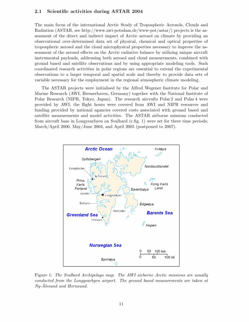
The ASTAR projects were initialised by the Alfred Wegener Institute for Polar andMarine Research (AWI, Bremerhaven, Germany) together with the National Institute ofPolar Research (NIPR, Tokyo, Japan). The research aircrafts Polar 2 and Polar 4 wereprovided by AWI, the flight hours were covered from AWI and NIPR resources andfunding provided by national agancies covered costs associated with ground based andsatellite measurements and model activities. The ASTAR airborne missions conductedfrom aircraft base in Longyearbyen on Svalbard (c.fig. 1) were set for three time periods;March/April 2000, May/June 2004, and April 2005 (postponed to 2007).

Figure 1: The Svalbard Archipelago map. The AWI airborne Arctic missions are usuallyconducted from the Longyearbyen airport. The ground based measurements are taken atNy-Alesund and Hornsund.

11

The ASTAR 2000 campaignThe main goals of the ASTAR 2000 were the airborne measurements of the aerosol pa-

rameters of climate relevance (extinction coefficient, absoprtion coefficients, and scatteringphase function) and creation of the Arctic Aerosol Data Set (AADS) for future applicationfor climate impact studies by using the AWI regional climate model HIRHAM (Dethloffet al. [20]), as well as the comparison of these results with the ground based Raman lidarand the SAGE II satellite instrumentation (Treffeisen at al. [63]). The Polar 4 aircraftmeasurements were performed form Longyearbyen, while the simultaneous ground basedmeasurements in Ny-Alesund.

During the campaign new systems were used, like the ground based Raman lidar(Schumacher [64]), the star photometer (Herber at al. [65]), the tethered balloon, andan onboard absorption photometer. For the Arctic spring, 18 extinction profiles cover-ing background and various Arctic Haze conditions were collected with the Polar 4 and12 extinction profiles were obtained close to Ny-Aalesund with additional ground basedmeasurements. Based on these measurements the tropospheric Arctic aerosols and theirclimate impact was analysedwith the HIRHAM model (Rinke et al. [21]).

The ASTAR 2004 and 2005 campaignsFor both ASTAR 2004 and 2005 campaigns, 160 - 200 flight hours were allocated to

be shared by both involved aircrafts Polar 2 and Polar 4. However, due to an accidentof the Polar 4 aircraft during hard landing at the British Rothera Base at the AntarcticPeninsula in January 2005, the last campaign was postponed until April 2007.

During both missions three major issues are approached. Firstly, in May/June 2004typical clean Arctic summer conditions with characteristic sea salt and mineral aerosolloads protected from long range transport of polluted air. Secondly, in April 2007 typicalArctic Haze event of strong intrusion of an antropogenic origin polluted air mass from lowerlaltitudes during winter conditions and a transition into the clean Arctic summer. Thirdly,the combination of results from both measurement periods for the determination of ananthropogenic influence on the radiative balance including the cloud formation processes.

The list of participating institutes separated according to the type of activities duringASTAR 2004 campaign is presented in figure 2.

In the frame of both of these campaigns the Lidar Group of AWI Potsdam contributeshigh quality measurements of tropospheric aerosols, using an especially for this purpose de-signed Airborne Mobile Aerosol Lidar (AMALi) integrated on board of the Polar 2 researchaircraft (Stachlewska et al. [66]), providing information on the existence, backscatter anddepolarisation of the vertical and horizontal extent of Arctic aerosols and/or mixed-phaseclouds of low optical densities.

2.1.1 Airborne activities

The Polar 2 and Polar 4 airborne operations were carried out from Longyearbyen startingon 7 May 2004. The scientific routine flight operation with both aircrafts started on May18 and finished on June 10. All flights were carried out without any unusual occurrencesproviding 120h 20 min of measurement data.

The scientific equipment installed onboard was certified, according to the Germanregulations for aircraft operation, by DLR officials after approval of documents describingthe scientific aim, measuring principle and technical description including the instrumentscheme with a list of all devices where their size, weight, centre of gravity and requiredpower consumption were specified. Also the calculations for the stability proof, the locationplan of all components and cables inside the aircraft’s cabin and wings, the block diagram

12

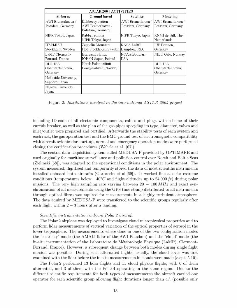
Figure 2: Institutions involved in the international ASTAR 2004 project

including ID-code of all electronic components, cables and plugs with scheme of theircurcuit breaker, as well as the plan of the gas pipes specyfing its type, diameter, valves andinlet/outlet were prepared and certified. Afterwards the stability tests of each system andeach rack, the gas operation test and the EMC ground test of electromagnetic compatibilitywith aircraft avionics for start-up, normal and emergency operation modes were performedclosing the certification procedures (Wehrle et al. [67]).

The central data acquisition system called MEDUSA-P provided by OPTIMARE andused originally for maritime surveillance and pollution control over North and Baltic Seas(Zielinski [68]), was adapted to the operational conditions in the polar environment. Thesystem measured, digitlised and temporarily stored the data of most scientific instrumentsinstalled onboard both aircrafts (Garbrecht et al.[69]). It worked fine also for extremeconditions (temperatures below −40◦C and flight altitudes up to 24.000 ft) during polarmissions. The very high sampling rate varying between 20 − 100 MHz and exact syn-chronisation of all measurements using the GPS time stamp distributed to all instrumentsthrough optical fibres was aquired for measurements in a highly turbulent atmosphere.The data aquired by MEDUSA-P were transferred to the scientific groups regularly aftereach flight within 2 − 3 hours after a landing.

Scientific instrumentation onboard Polar 2 aircraftThe Polar 2 airplane was deployed to investigate cloud microphysical properties and to

perform lidar measurements of vertical variation of the optical properties of aerosol in thelower troposphere. The measurements where done in one of the two configuration modesthe ’clear-sky’ mode (the AMALi lidar of the AWI-Potsdam) and the ’cloud’ mode (thein-situ instrumentation of the Laboratoire de Meteorologie Physique (LaMP), Clermont-Ferrand, France). However, a subsequent change between both modes during single flightmission was possible. During such alternated flights, usually, the cloud cover was firstexamined with the lidar before the in-situ measurements in clouds were made (c.cpt. 5.10).

The Polar 2 performed 13 lidar flights and 11 cloud physics flights, with 6 of themalternated, and 3 of them with the Polar 4 operating in the same region. Due to thedifferent scientific requirements for both types of measurements the aircraft carried oneoperator for each scientific group allowing flight durations longer than 4h (possible only

13

for the Arctic configuration with wheel operation) at the maximum flight altitude set to3 km (10.000 ft) due to lack of oxygen breathing system onboard.

Three racks installed perpendicularly to the axis of the aircraft were imployed, withthe first two reserved for the LaMP instrumentation and the AMALi lidar, while thethird one contained the AWI meteorological and radiation sensors and the MEDUSA-P acquisition unit. The CO - analyser was installed next to the lidar Optical Assemblymounted at the opening in the front section of the cabin. The lidar operational range waslimited to 2.5 km with respect to eye-safety of observers on the ground (c.cpt. 3). Othersecurity features as a laser emergency switch, a labelling of the laser, a key off-switch,and screws secured with safety wires had to be employed. The lidar was connected to theaircraft power distribution by 5 plugs (3 x 220V , 2 x 28 V ) compatible with the aircraft’sstandard provided by OPTIMARE. The data acquisition and storage was done with a lidarnotebook. The lidar data backup by MEDUSA-P was not provided, however, the timestamp (RS 232 with 1Hz), the online GPS data and (after each flight) an ASCII-data fileof navigation and basic meteorology were provided. An overview of the instrumentationonboard the Polar 2 aircraft is presented in figure 3.

Figure 3: Instrumentation onboard Polar 2 during ASTAR 2004 campaign

The AWI’s AMALi lidar (c.cpt. 3), was operated without any problems during all 13flight delivering about 25h of lidar measurements. The extended observations taken atdifferent days covered: the aerosol boundary layer and clouds over Isfjorden, Kongsfjorden,Advantdalen, and Storfjorden, few cross-sections over sea along NW-SE off the Svalbardcoast line with wave-driven aerosol structures and aerosol gradients between different airmasses, different aerosol content over ice and open water and the local dust plume overAdventdalen and Isfjorden. During two flights over Kongsfjorden and Storfjorden lidarmeasurements were partly combined with in-situ aerosol profile measurements taken byPolar 4 aircraft. One flight, partly combined with measurements at the Polish researchstation in Hornsund, was dedicated to investigations of air masses along the west andeast coast offshore Sorkappland. Additionaly, several combined measurements betweenthe AMALi lidar and the stationary KARL lidar over Koldewey station in Ny-Alesundwere performend. The detailed information on each of the ASTAR 2004 AMALi flightscan be found in Stachlewska and Neuber [70].

The LaMP’s in-situ instrumentations (c.cpt. 5.10.2) used for the measurements of themicrophysical and optical properties of cloud particles provided characterisation of the

14

mixed-phase of the Arctic clouds, with special focus on the investigation of the differentice crystal shape confined to distinct zones of the cloud systems. The cloud instrumen-tation worked fine during all flights except for May 29, when heavy icing of the PolarNephelometer occurred while measuring in a supercooled stratocumulus deck. Severalalternated measurements with AMALi dedicated to investigations of clouds structures off-shore the west coast of Prins Karls Forland, Albertland and in the Storfjorden allowed forthe feseability study of the depolarisation effects in lidar signals due to presence of the icecrystals in the sampled cloud areas (c.cpt. 5.10). One of the alternated AMALi/LaMPflights combined with an aerosol in-situ measurement from Polar 4 was dedicated to thestudy of the activation of aerosol particles to cloud droplets and ice crystals.

Scientific instrumentation onboard Polar 4 aircraftThe scientific equipment of the Polar 4 aircraft was used to investigate the physical,

chemical and optical properties of aerosol throughoutthe whole troposphere under clearsky conditions. Polar 4 performed 25 aerosol flights carrying equipment of three differentscientific groups onboard, each with an operator, which restricted flight duration to amaximum of 2 h 45 min. The operation up to 8 km (24.000 ft) with the oxygen breathingsystem onboard was possible.

The instrumentation onboard Polar 4 aircraft consisted of aerosol remote and in-situinstrumentation, and a standard meteorological and radiation imstrumentation (c.fig. 4).Four racks were employed: the first one, installed parallel to the axis of the aircraft, wasreserved for the DLR-IPA instrumentation, while the next three, installed perpendicu-larly to the axis of the aircraft, were reserved each for the ITM/MISU, the NIPR, andthe MEDUSA-P with the AWI radiation units, respectively. The sunphotometerand theCO2-system were installed in the front part of the cabin. In order to reduce the powerconsumption onboard, the DLR-IPA and ITM/MISU instruments shared one pump fortheir inlets (the DLR-IPA FSSP-100 probe was kept as a backup system only), and theflow rate required by the NIPR inlet was reduced to 10 l min−1, values comparable withITM/MISU and DLR-IPA inlets. The MEDUSA-P online meteorological data (especiallyan on-line true air speed indicator) were required by all systems, while the time stampwas not.

Both of the AWI instruments (sunphotometer and ozone analyzer), and the NIPRpayloads worked without trouble, with exception of the latter one during the iceing eventon May 29. The ITM/MISU and the DLR-IPA payloads worked fine, except on May 24when two of four CPSA channels failed due to the Butanol flooding of the optics. Somemarginal data loss of both the DLR-IPA and the ITM/MISU payloads occurred duringthree flights due to hard disk problems.

The aerosol measurements onboard Polar 4 covered mainly the vicinity of Isfjorden andthe area over the sea west of Prins Karls Forland. Several flights were devoted to measureaerosol vertical profiles in Kongsfjorden and just offshore its mouth from the flight level of60 m in the marine boundary layer up to 7 km in the free troposphere. Generally, duringthe whole campaign typical background conditions with low values of aerosol concentra-tions and extinctions and low variability were found throughout the troposphere duringmost of the flights (c.cpt. 5.6.1).

2.1.2 Ground based, satellite and modelling activities

Ground based activitiesThe coordinated ground based activities took place in vicinity of Ny-Alesund, namely

at the AWI Koldewey Station, the Japanese Rabben Station and the Swedish ZeppelinMountain Station, as well as at the Polish Research Station in Hornsund on the west coastof Sorekapland (c.fig. 1).

15

Figure 4: Instrumentation onboard Polar 4 during ASTAR 2004 campaign

All of these research stations provided the meteorological parameters wind, pressure,humidity and temperature and the measurements of optical and microphysical atmosphericproperties (Herber et al. [65]). An overview of the measurements performed at the stationsin Ny-Alesund and Hornsund are given in figures 5 and 6, respectively.

The in-situ and remote ground based measurements generally confirmed the airborneobservations. The clean conditions manifested in the low amounts of light absorbingparticles (soot), very low concentrations of large particles, the low aerosol optical depthobtained from the sunphotometer and background values of backscatter and extinctioncoefficients. Generally, very low volumne depolarisation recorded by KARL lidar justifiedthe existence of only spherical particles (c.cpt. 5.6.1).

Satellite activitiesThe satellite observations (ATSR-2, ENVISAT/SCIAMACHY, ILAS II, MERIS, MODIS,

OMI, SAGE III, SeaWiFS) with their high speed and global range complete the local mea-surements of the polar aircrafts and hence link local, regional and global processes. Duringthe field campaigns their imagery is used on a daily basis for the general weather situationassessment and for pre-defining the areas where clear-sky and cloud measurements can be

16

Figure 5: Instrumentation in viscinity of Ny-Alesund during ASTAR 2004 campaign

carried out.With respect to aerosol investigations, the validation of the satallite aerosol optical

depth by the direct comparison with the airborne measurements (Treffeisen et al. [63])allows for improvement of present algorithms of satellite retrievals for the aerosol opticalthickness for high latitudes and low sun elevations in the Arctic (von Hoyningen-Hueneet al. [23], Kokhanovsky et al. [71]). Hence, the regional extension of Arctic aerosolproperties, necessary for the future modelling will be determined.

Modelling activities during the campaignDuring the campaign, mainly the results of the European Centre for Medium-Range

Weather Forecasts model (ECMWF, http://www.ecmwf.int/) were used for prediction ofthe synoptic scale and medium range weather forecasted for 726h on a 6 h scale. Theprediction was provided in terms of the dynamics charts with respect to the potentialvorticity and sea level pressure; the clouds charts for low (below 800hPa), mid (between400 − 800 hPa), and high (above 400hPa) cloud altitude, as well as the cloud partitioningwith respect to the ice and water content. Finally, the meteorological charts includedrelative humidity, temperature, geopotential and wind. Additionally, forecast meteograms

17

Figure 6: Instrumentation of the Hornsund station during ASTAR 2004 campaign

of total cloud cover, total precipitation, wind speed and temperature were provided forthree locations; Ny-Alesund, Longyearbyen and just offshore Hornsund.

The combination of the ECMWF forecast (provided by A. Dornbrack, DLR-IPA, Ger-many), the forecasted 3-dim backward trajectories (provided by P. van Velthoven, KNMI,The Netherlands), the aerosol optical depth MATCH CTM model forecast (provided byP. Rash, NCAR, USA), the satellite imagery by MODIS, NOAA, combined with the dailyflight-weather briefing (presented by L. Bergstadt, AVINOR, Svalbard) was used for thescientific decision-making concerning the flight activities.

On the other hand to explain the weather situation and the processes occuring inthe atmosphere for particularly interesting weather events the results of the ECMWFoperational analysis were used (c.cpt. 5.1).

The origin of the measured aerosol load with respect to its long-range transport wasdetermined using the two trajectories models NOAA HYSPLIT (Draxler and Rolph [72])and a particle dispersion model FLEXPART (Stohl et al. [73]).

The interpretation of the aerosol load with respect to its local origin was providedusing the small-scale range dispersive EULAG model (Prusa and Smolarkiewicz [74], andSmolarkiewicz and Prusa [75]).

The regional atmospheric climate model HIRHAMThree main issues are of concern for the post-campaign modelling. Firstly, an estima-

tion of the climate effect caused by antropogenic aerosol (Arctic Haze) versus backgroundconditions calculated for solar and terrestrial radiative balance modelled with differentcomplexity. Secondly, the studies of the relevance of aerosol properties in arctic climatemodels by comparison of the aerosol effect to other forcing mechanisms to see its rela-tive impact. Thirdly, the development of parameterisations of aerosol and cloud processesbased on provided remote or in-situ observations.

The high resolution 3-dim regional atmospheric climate model HIRHAM (HIRHAM,http://www.awi-potsdam.de/www-pot/hirham), see: Dethloff et al. [20], Dethloff et al.[76], Rinke and Dethloff [77]) with the incorporated Global Aerosol Data Set (GADS) andthe Arctic Aerosol Data Set (AADS) developed at ASTAR 2000 campaign used over anarea covering the whole Arctic north of 65◦N and integrated over a spring season of typicalArctic Haze reveal the realistic estimation on the direct effect of Arctic Haze on climate(Fortmann [37]). Moreover, the indirect influence on the large-scale and the meso-scaleatmospheric circulation due to the aerosol-radiation-circulation feedback, as for examplethe scattering and absorption of radiation by aerosol, can cause pressure pattern changes

18

potentially able to modify Arctic teleconnection patterns (Rinke et al. [21]).Similar modelling will be performed in the future for the ASTAR 2004 and 2007 cam-

paigns, including new informations obtained from the airborne AMALi aerosol and cloudsmeasurements and the airborne in-situ clouds observations performend onboard the Po-lar 2 aircraft. The campaigns will provide detailed data sets of optical parameters of ArcticHaze and Arctic clouds which will be used for parameterisation of such aerosols and cloudsin the HIRHAM model, for which both parametrisations are still in the development phase.

2.2 Scientific activities during SVALEX 2005

The airborne activities of the Svalbard Experiment (SVALEX) campaign utilising theAWI research aircraft Polar 2 and the DLR research aircraft D-CFFU were conductedfrom Longyearbyen on Spitsbergen between 5 - 22 April 2005.

The Polar 2 aircraft was deployed during almost 20 flight hours for measurementsof the ice surface structure and atmospheric turbulence above the ice shield to providea parametrisation of the turbulent transport of energy and momentum for climate andweather models (Garbrecht et al. [78]). These investigations were combined with theD-CFFU aircraft radar measurements of the thickness, structure and surface of sea andland ice with almost 33 hours of observations for this activity.

Additionally, the SVALEX campaign aimed to deal with the characteristics of an in-creased springtime tropospheric aerosol load typical for an Arctic Haze event and inves-tigations of its effects on climate. The AMALi lidar onboard Polar 2 provided almost 20hours of measurements allowing to determine the optical characteristics of such aerosoland its spatial (in)homogeneity and distribution. At the same time the aim of the groundbased measurements was, similarly to the ASTAR 2004 campaign, to provide a com-prehensive characterisation of the temporal and vertical distribution of Arctic Haze overNy-Alesund using the Koldewey Aerosol Raman Lidar (KARL), the sun photometer run-ning in automatic mode and delivering the aerosol optical depth spectrum from UV tonear IR.

The optical depth spectra were measured also with a sun photometer in Longyearbyen.Additionally, the radio/ozone soundings and the meteorological measurements were per-formed by the staff of the Koldewey Station. Furthermore, the chemical characterisationof low altitude aerosols using combined MicroPulse Lidar observations with the measure-ments of the chemical state of surface layer aerosol, and the investigations of precipitationwere performed by NIPR instrumentation at the Koldewey and Rabben Stations.

The weather prediction for the next hours/days provided by AVINOR together with theMODIS and NOAA satellite imagery and predicted trajectories provided by KNMI allowedfor the scientific planning of each flight mission. Afterwards the long-range transportanalysis was made with help of the NOAA HYSPLIT backtrajectories, while for particulardays also the FLEXPART calculations were performed (c.cpt. 5.6)

Due to unfavourable weather conditions and according technical problems, the testflight operations started only on 8 April for Polar 2 and on 12 April for D-CFFU. Generally,weather conditions often limited aircraft activities due to cloud ceiling, visibility, crosswind, snowfall and snowstorms. However, the AMALi scientific operation was possible on4 days of clear-sky conditions between 12 - 16 April.

In total 18h 30 min flight observations were performed with 13 successful overflightsover Ny-Alesund in order to allow the combination of the KARL and AMALi data setsand the other supporting ground based measurements. During these 4 days, an ArcticHaze event was clearly seen from the measurements with both AMALi and KARL lidars,as well as with both sunphotometers in Longyerbyen and Ny-Alesund (c.cpt. 5.6 and 5.7.The detailed information on each of the AMALi flights can be found in Stachlewska [79].

19

3 AWI lidars for measurements during Arctic field cam-paigns

In the frame of the ASTAR 2004 and the SVALEX 2005 campaigns the Lidar Group of theAWI Potsdam Research Unit performed high quality measurements of the troposphericaerosols, using two lidar systems, the stationary zenith-aiming Koldewey Aerosol RamanLidar (KARL) and the nadir-aiming Airborne Mobile Aerosol Lidar (AMALi) integratedonboard the Polar 2 research aircraft. In this chapter a short description of the KARLlidar (c.cpt. 3.1) and a detailed description of the AMALi lidar (c.cpt. 3.2) are given.

3.1 The stationary Koldewey Aerosol Raman Lidar KARL

The Koldewey Aerosol Raman Lidar (KARL) was developed in 1998 by the AWI-PotsdamLidar Group (Schumacher [64]). It is a ground based system firmly integrated into theKoldewey station in Ny Alesund, Spitsbergen (78.9◦ N, 11.9◦E) aiming at continuous reg-ular detection of tropospheric aerosols and water vapour.

It consists of a Nd:Yag laser operating with 30Hz repetition rate at 355nm, linearlypolarised 532nm and 1064nm with power around 2W for each wavelength. The receiv-ing system employs two mirrors; a small telescope mirror of 10.8 cm diameter and fieldof view of 2.25mrad for near range detection from 400m to 6 km and a large telescopemirror of 30 cm diameter and field of view of 0.83mrad for far range measurements from2 km to above the tropopause. Detection is provided for the three wavelengths togetherwith depolarisation information for 532nm. Moreover, the N2 Raman-shifted wavelengthsof 387nm and 607nm, as well as the water-vapour lines of 407nm and 660nm can berecorded. The elastic scattering profiles are typically provided with 60m range resolutionand integration times over 10min when the standard automatised evaluation routine isapplied. The backscatter profiles are ranging from geometrical compression at approx-imately 400 m up to 15 km during daylight and 18 km at night.The inelastic scatteringprofiles for the Raman channels are provided generally with weaker resolution, due to themuch lower cross-section for Raman scattering in the atmosphere. Therefore a height res-olution of 300m for integration times over an hour is necessary. These profiles are rangingup to 4 km for the daytime and 8 km at nighttime measurements.

Since 1998 the system went through extended improvements towards development untoits present form, as for example the inclusion of water vapour and IR detection channelsin 1999 and UV detection channel in 2001. The exchange of the Nd:Yag laser for anew generation one operating with 50Hz repetition rateand emitting more powerful laserpulses of 1000 mJ at IR, 500 mJ at VIS, and 275mJ UV is planned for April 2006. Moreinformation about KARL and its application is given in Ritter et al. [80] and Ritter andNeuber [81].

3.2 The new Airborne Mobile Aerosol Lidar AMALi

The Airborne Mobile Aerosol Lidar (AMALi) was developed in 2003 by the AWI-PotsdamLidar Group (Stachlewska et al. [66]). This small robust easy to transport backscatterlidar (c.fig. 7) is used for remote simultaneous high resolution detection of vertical andhorizontal extent of tropospheric aerosol load at 1064nm and 532nm wavelength withadditional depolarisation measurements at the latter one. The lidar is mounted in twosmall, portable modules. An Optical Assembly (70×50×25 cm) comprises the laser head,directing and receiving optics, and electro-optical detectors. The laser control and coolingunit, the data acquisition system (laptop and transient recorders) and the safety breakerbox are installed in a standard size rack (55×50×60 cm).

20

Figure 7: The AMALi in nadir-airborne configuration onboard Polar 2 aircraft (right),inside of the optical assembly (left). The numbers indicate the main elements of theAMALi lidar; 1.optical assembly 2.laptop 3.safety breaker box 4.laser control and cool-ing unit 5.transient recorder.

The design of AMALi allows downward measurements in vertical direction for thecurrent configuration onboard AWI’s Polar/,2 aircraft. When the lidar is operated atthe ground level or integrated in a car or a ship, measurements are usually taken verti-cally upward (system is turned upside-down), however, horizontal measurements are alsopossible (system lying on a side). It can be used also in a scanning mode, if set on aplatform allowing movement of the whole system in vertical/horizontal direction. Despiteits relatively small size AMALi in ground based configuration is powerful enough to coverthe range up to the tropopause level. For airborne measurements its range is limited tothe maximum flight altitude, the maximum nominal operation height for the laser andeye-safety constraints.

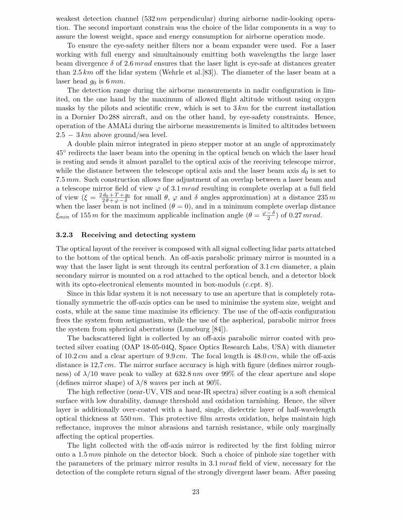
The rapid data acquisition system enables recording of lidar profiles with single-shotresolution providing high spatial and, hence, horizontal resolution information about thestate of the atmosphere between the flight altitude and the ground/sea level during themeasurement. The online, quick-look data evaluation software allows immediate, qualita-tive interpretation of the aerosol content during the flight, and thus guidance of a secondresearch aircraft for in-situ measurements into particularly interesting areas.

3.2.1 Optical assembly

The transmitting and receiving systems are mounted inside an optical assembly designedby AWI-Potsdam Lidar Group and manufactured by Steingross Feinmechanik, Berlin.This small, light weight module (70×50×25 cm, 38 kg) called optical assembly (c.cpt. 7,left) was designed especially to fit a limited space available for the lidar instrument onboard the Polar 2, the AWI research aircraft Dornier Do 228.

All vital lidar parts, i.e. Nd:Yag laser head, directing optics, receiving off-axis telescopemirror and detector block with its opto-electronical elements are mounted onto the sameoptical bench (c.cpt. 8). Such single-optical-bench design simplifies single-adjustment of alloptical elements and ensures reliable and trouble-free utilisation during campaigns withoutneed of re-adjustment. The optical bench itself hangs on anti-shock springs attached tofour posts. The springs eliminate vibrations of the optical bench while operation on boardof the aircraft. The weight and position of all elements (on the optical bench) are chosenin a way that the centre of gravity results in the middle of the optical assembly. Thefour posts together with a base plate form a massive construction providing mechanical

21

stability to the system. During measurements the optical assembly is covered with a sheetmetal box capturing any scattered laser light and thereby ensuring the safety of pilotsand operators, as well as protecting the detection system from stray light and backgroundradiation.

Figure 8: The AMALi optical assembly with schematically drawn ray-tracking at 532 nm(green) and 1064 nm (red). The numbers indicate the main components in the assembly;1.laser head 2.directing mirror in piezo motor 3.window with Brewsters angle 4.off-axisparabolic mirror 5.first folding mirror 6.pinhole 7.second folding mirror 8.achromatic lens9.beam splitter 10.interference filter for 1064nm channel 11.APD for 1064nm detection12.interference filter for 532 nm channel 13.polarising cube 14.thin film polarising filter15.PMT for perpendicular 532nm detection 16.PMT for parallel 532nm detection 17.op-tical bench 18.springs 19.posts 20.base plate.

3.2.2 Transmitting system

As a transmitter custom designed small rugged and easy to handle flashlamp pumpedNd:YAG pulsed laser (CRF-200, Big Sky Quantel, Montana, USA) is used. It is providedwith portable power supply and cooling unit mounted in a single, low weight (3 kg) andspace requirements (12×45×48 cm) unit. The laser, equipped with doubler crystal, emitssimultaneously 1064nm and linearly polarised 532nm wavelengths as 11 ns short lightpulses with energies of 60 mJ and 120mJ , respectively, with the pulse repetition rate of15 Hz.

The double wavelength backscatter lidar scheme was chosen for its conceptual simple-ness (Shimoda [82]) ensureing an easy and trouble-free operation during field campaignsunder tough conditions, as for example onboard of the AWI research aircraft Polar 2 dur-ing field campaigns in the Arctic. The laser is cooled with an ethylene glycol and water1:1 solution to ensure that the liquid will not freeze while the laser is operating underarctic weather conditions and at high altitudes, whereby the maximum nominal operationheight for the laser is set to 3 km.

The laser divergence δ, the telescope mirror diameter T and the pinhole diameter stogether with the laser pulse power and repetition rate were chosen with the constrain toachieve the lowest possible geometric compression ξ with lowest integration times for the

22

weakest detection channel (532 nm perpendicular) during airborne nadir-looking opera-tion. The second important constrain was the choice of the lidar components in a way toassure the lowest weight, space and energy consumption for airborne operation mode.

To ensure the eye-safety neither filters nor a beam expander were used. For a laserworking with full energy and simultainously emitting both wavelengths the large laserbeam divergence δ of 2.6mrad ensures that the laser light is eye-safe at distances greaterthan 2.5 km off the lidar system (Wehrle et al.[83]). The diameter of the laser beam at alaser head g0 is 6 mm.

The detection range during the airborne measurements in nadir configuration is lim-ited, on the one hand by the maximum of allowed flight altitude without using oxygenmasks by the pilots and scientific crew, which is set to 3 km for the current installationin a Dornier Do 288 aircraft, and on the other hand, by eye-safety constraints. Hence,operation of the AMALi during the airborne measurements is limited to altitudes between2.5 − 3 km above ground/sea level.

A double plain mirror integrated in piezo stepper motor at an angle of approximately45◦ redirects the laser beam into the opening in the optical bench on which the laser headis resting and sends it almost parallel to the optical axis of the receiving telescope mirror,while the distance between the telescope optical axis and the laser beam axis d0 is set to7.5 mm. Such construction allows fine adjustment of an overlap between a laser beam anda telescope mirror field of view ϕ of 3.1mrad resulting in complete overlap at a full fieldof view (ξ = 2 d0 + T + g0

2 θ + ϕ− δ for small θ, ϕ and δ angles approximation) at a distance 235mwhen the laser beam is not inclined (θ = 0), and in a minimum complete overlap distanceξmin of 155 m for the maximum applicable inclination angle (θ = ϕ− δ

2 ) of 0.27mrad.

3.2.3 Receiving and detecting system

The optical layout of the receiver is composed with all signal collecting lidar parts attatchedto the bottom of the optical bench. An off-axis parabolic primary mirror is mounted in away that the laser light is sent through its central perforation of 3.1 cm diameter, a plainsecondary mirror is mounted on a rod attached to the optical bench, and a detector blockwith its opto-electronical elements mounted in box-moduls (c.cpt. 8).

Since in this lidar system it is not necessary to use an aperture that is completely rota-tionally symmetric the off-axis optics can be used to minimise the system size, weight andcosts, while at the same time maximise its efficiency. The use of the off-axis configurationfrees the system from astigmatism, while the use of the aspherical, parabolic mirror freesthe system from spherical aberrations (Luneburg [84]).

The backscattered light is collected by an off-axis parabolic mirror coated with pro-tected silver coating (OAP 18-05-04Q, Space Optics Research Labs, USA) with diameterof 10.2 cm and a clear aperture of 9.9 cm. The focal length is 48.0 cm, while the off-axisdistance is 12,7 cm. The mirror surface accuracy is high with figure (defines mirror rough-ness) of λ/10 wave peak to valley at 632.8 nm over 99% of the clear aperture and slope(defines mirror shape) of λ/8 waves per inch at 90%.

The high reflective (near-UV, VIS and near-IR spectra) silver coating is a soft chemicalsurface with low durability, damage threshold and oxidation tarnishing. Hence, the silverlayer is additionally over-coated with a hard, single, dielectric layer of half-wavelengthoptical thickness at 550nm. This protective film arrests oxidation, helps maintain highreflectance, improves the minor abrasions and tarnish resistance, while only marginallyaffecting the optical properties.

The light collected with the off-axis mirror is redirected by the first folding mirroronto a 1.5mm pinhole on the detector block. Such a choice of pinhole size together withthe parameters of the primary mirror results in 3.1mrad field of view, necessary for thedetection of the complete return signal of the strongly divergent laser beam. After passing

23

the pinhole the light is redirected using the second plane folding mirror to an achromaticlens used to produce parallel rays while avoiding chromatic aberration (Luneburg [84]).

The signals of both frequencies are separated into two different detection channels us-ing a dichroic mirror inclined at 45◦ which transmits the 1064nm and reflects the 532 nmsignal. The last wavelength is additionally separated into its parallel and perpendicularcomponent using a polarising cube beam splitter. In front of the photo-detectors interfer-ence filters are placed to reduce the background daylight radiation. For the IR channel a1.0 nm wide interference filter centred around 1064nm is used, and for both VIS channelsa 0.15 nm wide interference filter centred around 532nm. Due to the limited range of theairborne signals a strong peak of the ground return occures. However, the use of absorp-tive neutral density filters to reduce the intensity of the incoming light is not necessary.The less intense, perpendicular component of the 532nm channel is additionally filteredfor cross-talk using a thin film polarising filter at a 56◦ angle.

3.2.4 Data acquisition system

A single laptop computer (TOSHIBA, 2GHz, CPU 30 GB, HD 256 MB RAM, USB-RS 232, Windows XP-Pro, OPS english) fully controls the laser, transient recorders, detec-tors, and data acquisition, storage, processing, quick-look evaluation and display programsutilising LabVIEW software. As data acquisition system a transient recorder (TR20-80,LICEL GbR, Berlin) combining an A/D converter (12 bit at 20 MHz) for analog detec-tion with a 250MHz fast photon counting system is used. An ethernet control moduleusing a TPC/IP protocol allows remote control and data transfer for both photon count-ing and analog recorders. For the detection of the 1064nm channel a Peltier cooled SiAvalanche Photo-Diode (APD) is used, and for the detection at both 532nm channels twoHamamatsu R7400 photomultipliers (PMT).

Transient recorders register the pulses with a maximum sampling rate of 20 MHzcorresponding to a height resolution of 7.5m for one range bin. In a nadir-aiming airborneconfiguration typically each new lidar return signal from each of the three channels isappended and stored with a time resolution of 1 s in a block file of 2min. However, aresolution as fine as a single-shot acquisition is also possible.

In a zenith-looking ground based configuration a standard LICEL software is employed.Here each new lidar return signal from each channel is stored separately at a time resolutionof minimum 1 s and hence, a single-shot acquisition is not possible. With this standardsoftware the profiles up to the tropopause level can be easily obtained.

For the nadir-airborne applications an custom designed LICEL software is employed.Here, the length of each collected signal is limited to 1000 range bins (7.5 km) to decreasethe time needed for data transfer between transient recorder and the laptop (smaller sizeof data files). At the same time, it provides sufficient number of bins for the requiredrange determined by the altitude of the flying aircraft for nadir-aiming configuration, i.e.maximum of 3 km above sea level. For this short distance (significantly shorter than thezenith-aiming ground based range), a strong received signal with sufficient signal-to-noiseratio is guaranteed, so that the photomultipliers can be operated in an analog mode only(Goodman [85]).

Additionally, the measurements in nadir airborne configuration generally provide abetter signal-to-noise ratio at far distances from the aircraft, as the measured aerosolconcentration and the air density increases towards the ground. On the other hand, forthe airborne applications only short integration times are allowed in order to achievean sufficient horizontal resolution. An acceptable signal-to-noise ratio is achieved for anintegration time of 1 s corresponding to a horizontal resolution between 46m and 77mat a minimum of 166 km/h (90 kt) and maximum of 278 km/h (150 kt) aircraft cruisingspeed over ground, respectively.

24

The limited range of the recorded airborne signals results in a difficulty to obtain thebackground light intensity, which has to be subtracted for the evaluation of the lidar data.To overcome this problem, the data acquisition is started by an adjustable pretrigger tothe laser Q-switch, designed by LICEL especially for the AMALi airborne applications.The timing of the pretrigger is usually chosen up to a value of 25μs corresponding to 500range bins (3750m) of the signal (c.cpt. 9).

Figure 9: The AMALi adjustable pretriggering scheme. The timing of the pretrigger canbe chosen up to a maximum of 26μs.

The lidar profiles are stored on the laptop and provide information about the state ofthe atmosphere between the full overlap and the ground or sea level during the flight.Theycan be viewed online during the flight using a special designed feature of so called quick-look evaluation screen in the data acquisition programmes. Each second one of the dis-play screens provide all three currently measured raw signal profiles. Similarly, threeother screens are frequently updated with background and range corrected signal pro-files at both 1064nm and parallel 532nm channels, as well as with depolarisation ratio(532 nm perp./532nm par.) profiles, all averaged over 15 s.

This online quick-look data evaluation allows immediate ’first-guess’ interpretation ofthe aerosol data during the flight providing also sufficient information for an onboardlidar operator to, for example, guide another research aircraft for specific in-situ measure-ments. During the ASTAR 2004 campaign the quick-look evaluation feature allowed alsoto guide alternated Polar 2 measurements, i.e. after identification by lidar measurementsof particularly interesting regions of mixed-phase clouds (indication of height and rela-tive concentration of water droplets and/or ice crystals areas) the aircraft descended intospecified parts of these clouds for in-situ measurements of their microphyscial and opticalparameters (c.cpt. 5.10). An exemplary quick-look real-time evaluation displays obtainedduring this particular flight are shown in figure 10.

3.2.5 AMALi end-products and their applications

The AMALi lidar provides a high quality information on existence, altitude distribu-tion, backscatter and depolarisation of the vertical and horizontal extent of troposphericaerosols and low optical thickness clouds, by delivering profiles of the range and back-ground corrected signals, the aerosol backscatter coefficients, the aerosol particles non-sphericity (depolarisation information) and, by the remedy of additional information orinstrumentation, even the extinction coefficients.

As a first type end-product, for both nadir-looking airborne as well as zenith-lookingground based lidar configurations, profiles of background and range corrected signal forboth 1064nm and parallel 532nm channels and profiles of depolarisation ratio at 532nmare delivered. All these profiles are averaged over 1 s with range resolution of 7.5m andhorizontal resolution of 67m for typical aircraft’s cruising speed over ground of 130 kt.Typical length of airborne profiles vary between 2.5 - 2.7 km depending on flight altitudeand taking into account the 155 - 235m losses due to geometrical compression near thelidar. For the airborne measurements the background correction value for each profile isobtained from the pretrigger part of the signal and extracted from each profile separately.

25

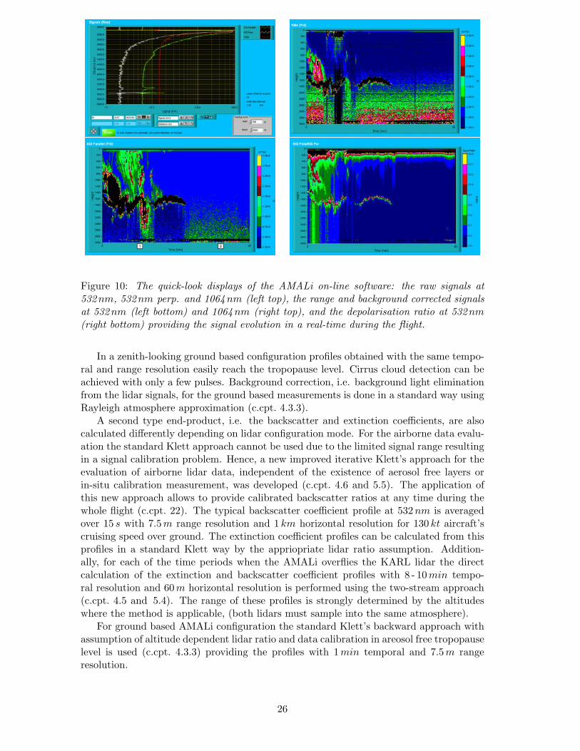
Figure 10: The quick-look displays of the AMALi on-line software: the raw signals at532nm, 532nm perp. and 1064nm (left top), the range and background corrected signalsat 532nm (left bottom) and 1064nm (right top), and the depolarisation ratio at 532nm(right bottom) providing the signal evolution in a real-time during the flight.

In a zenith-looking ground based configuration profiles obtained with the same tempo-ral and range resolution easily reach the tropopause level. Cirrus cloud detection can beachieved with only a few pulses. Background correction, i.e. background light eliminationfrom the lidar signals, for the ground based measurements is done in a standard way usingRayleigh atmosphere approximation (c.cpt. 4.3.3).

A second type end-product, i.e. the backscatter and extinction coefficients, are alsocalculated differently depending on lidar configuration mode. For the airborne data evalu-ation the standard Klett approach cannot be used due to the limited signal range resultingin a signal calibration problem. Hence, a new improved iterative Klett’s approach for theevaluation of airborne lidar data, independent of the existence of aerosol free layers orin-situ calibration measurement, was developed (c.cpt. 4.6 and 5.5). The application ofthis new approach allows to provide calibrated backscatter ratios at any time during thewhole flight (c.cpt. 22). The typical backscatter coefficient profile at 532nm is averagedover 15 s with 7.5 m range resolution and 1 km horizontal resolution for 130 kt aircraft’scruising speed over ground. The extinction coefficient profiles can be calculated from thisprofiles in a standard Klett way by the appriopriate lidar ratio assumption. Addition-ally, for each of the time periods when the AMALi overflies the KARL lidar the directcalculation of the extinction and backscatter coefficient profiles with 8 - 10min tempo-ral resolution and 60m horizontal resolution is performed using the two-stream approach(c.cpt. 4.5 and 5.4). The range of these profiles is strongly determined by the altitudeswhere the method is applicable, (both lidars must sample into the same atmosphere).

For ground based AMALi configuration the standard Klett’s backward approach withassumption of altitude dependent lidar ratio and data calibration in areosol free tropopauselevel is used (c.cpt. 4.3.3) providing the profiles with 1min temporal and 7.5m rangeresolution.

26

4 Data evaluation schemes and error sources discussion

Obtaining information on optical properties of aerosol particles in the atmosphere, i.e.obtaining extinction αpart and backscatter βpart coefficients profiles independently fromeach other without an assumption of lidar ratio B = αpart

βpart , signifies a great step forwardinto interpretation of lidar data. The aerosol particle microphysical parameters, i.e. theparticle index of refraction m and the size distribution function σ, can be derived form a setof αpart and βpart profiles obtained for different wavelengths (Muller et al. [86], Bockmann[87], Veselovskii et al. [88]) with the help of the generalized Lorenz-Mie theory (GLMT)of an arbitrary shaped beam of light scattered by homogeneous isotropic spheres derivedby Lorenz and, independently, Love [89], Mie [90], and Debye [91]. Gouesbet and Grehan[92] propose a similar theory built by the synthesis of the GLMT and the interactiontheory between a plane wave and assemblies of spheres and/or aggregates. The theory onelectromagnetic radiation interaction with arbitrarily shaped and oriented small particleswas recently revised by Mishchenko et al. [93]).

Such calculation, however, consists of a mathematically ill-posed inversion problem(Bronsztejn and Siemiendiajew [94]). The emergent Lorenz-Mie efficiencies act differentlyfor extinction and backscatter, hence, any inversion of microphysical parameters feededwith both coefficients calculated independently can be performed more precisely, espe-cially for the determination of the particle size distribution (Bockmann [87], Bockmannet al. [27]). Unfortunately, an elastic backscatter lidar alone cannot provide completeinformation for such an inversion, due to the existence of two unknowns, the α and β co-efficients, in only one equation discribing the lidar return signal (c.eq. 5). The traditionalKlett approach for the evaluation of elastic backscatter lidar data requires knowledge orassumption of the lidar ratio and an extinction or backscatter coefficient calibration value(Klett [28], [29]). For the numerically stable backward Klett-Fernald solution (c.cpt. 4.3.3)the appriopriate choice of a height and wavelength dependent lidar ratio B(h, λ) is cru-cial to provide accurate αpart and βpart profiles. Such proper choice is difficult since theactual lidar ratio of aerosol is usually not very well known in the troposphere and variesgreatly with aerosol size and its chemical composition. Generally, it is larger for intrinsicdark particles, as soot, and for particles small in comparison to the employed wavelength(Ackermann [95]).

The inclusion of a Raman-shifted detection line in the lidar instrument provides theneeded independent information (c.cpt. 4.4) and allows the direct retrieval of extinctionand backscatter (Ansmann et al. [96]). However, the cross-section for the Raman-shiftedinelastic scattering, so called Raman scattering (Demtroder [97]) of laser light by matter,is almost three orders of magnitude lower than the cross-section for the elastic interaction,i.e. the Lorenz-Mie scattering or the Rayleigh scattering (Rayleigh [98], Young [99]), whichresults in significantly more noise polluted signals.

Another approach providing such an independent information, the two-stream inver-sion (c.cpt. 4.5), also referred to as bipath or double-ended lidar method, requires the usageof two elastic backscatter lidar systems looking into opposite directions. The method, in-troduced by Kunz [31] and recently revised by Cuesta and Flamant [34], is considered tobe applicable not only to the airborne lidar data evaluation but also for future evaluationand validation of satellite lidar data. Though the method was already applied to oppositelooking lidars by Hughes and Paulson [32] and Jørgensen et al. [100], only very recently thefirst application of this approach to real airborne and ground based lidar data by Stach-lewska et al. [33] demonstrated its feasibility. The two-stream approach allows the directretrieval of the height dependent extinction coefficient without any a priori assumptions,normalisation or calibration. The only prerequisite to calculate the backscatter coefficientis knowledge of, usually unknown, lidar constants C of the employed intruments or abackscatter value βref at any given height in the measured interval (c.cpt. 4.5).

27

The instrumental constants of both a ground based CK and an airborne CA lidar,which usually are difficult to obtain, can be easily estimated within a few percent uncer-tainty, in the case that one of the lidars observes any aerosol poor layer, as for example inthe tropopause. Finally, with knowledge of the calibration constant of the airborne lidarCA it is possible to retrieve the calibrated airborne lidar backscatter coefficient profilesfor measurements taken during the whole flight, even in case when backscatter calibrationinstrumentation and/or laser beam scanning facilities are not available onboard (Stach-lewska et al. [36]).

4.1 Backscatter lidar techniques

Lidar techniques belong to the remote systems based on emission and detection of waves(light, radio, sound or ultrasound) using the instrument itself for transmiting and receivingbackward reflected waves (Measures [26], Andrews [101], Jensen [22]). In case of lidar laserlight pulses, consisting of one or more wavelengths, are transmitted into the atmospherevertically or at a particular angle θ. They interact with and are changed by atmosphericmolecules and particles causing alterations in the light intensity and wavelength accordingto the strength of optical interaction and the concentration of the interacting species inthe atmosphere. Some of the light is scattered back from the target to the lidar instrumentwhere the return signal is collected using a telescope mirror. The change in the proper-ties of the light enables some information of the target and, consequently, characteristicattributes of the composition and physical state of the atmosphere can be deduced fromthe lidar data.

Backscattering and extinction are the only optical processes measured by the system.The signals are mainly due to the elastic scattering (λem = λdet) on any air molecules

and tiny particles for which the particle size a is much smaller than the emitted wavelengtha < 0.1 λem in case of the Rayleigh scattering, and on particles, such as aerosols and dust,for which a ∼= λem in case of the Lorenz-Mie scattering. The relatively high cross-sectionfor these types of scattering makes the signal detection easy and suites the elastic scatteringlidars as very valuable for observations of the aerosol vertical distribution, since alreadysimple backscatter signals at almost any lidar wavelength give a qualitative impressionabout the vertical distribution of the scatterers.

Apart from mentioned elastic lidars, for which emission and detection are done forthe same laser wavelengths, inelastic (Raman) lidars are widely used in the Europeanlidar comunity (Matthias et al. [102], Bosenberg and Matthias et al. [25]). The Ramanaersol lidar uses the inelastic scattering principle with λem �= λdet, for which an additionaldetection is done for the backscattered signal at a Raman-shifted wavelength of a particularmolecule (Goldsmith et al. [103]). Due to the very weak cross-section for Raman scattering(10−32 − 10−35 cm2) usually the inelastic interaction of laser pulses with O2 and/or N2

molecules is used, taking the advantage of their high concentrations and large procentagein the air in comparison with other gaseous species, i.e. 21% and 78%, respectively. Inthese systems the energy shift towards the red or blue spectral range of Raman scatteringdepends on the incoming frequency of the photon and the molecule type. Usually, thedetection is done for the wavelength of the strongest shifted return, i.e. for a N2 moleculeilluminated by 532 nm light, the strongest lines occur at a shift of 75 nm and for O2 of48 nm, both towards red light (Stokes shift).

The analysis of registered lidar signals allows the retrieval of α and β, and the determi-nation of the concentration and type of aerosol. In the case of measurements with a set ofwavelengths it is also possible to determine the size distribution of particles (Rajeev andParameswaran [104]). Additionally, the detection of depolarisation of the backscatterdlight, i.e. detection of height dependent depolarisation ratio profiles, allows an estimationof the state of the particles interacting with light. The depolarisation ratio is defined

28

as the ratio between the reflectivity received at vertically polarised wavelength λ⊥, buttransmitted with horizontally polarised wavelength λ‖, and the reflectivity at horizontalpolarisation, i.e. D(h) = λ⊥

λ‖. The depolarisation of the horizontally polarised pulse is

caused by non-spherical particles not aligned horizontally. The wet spherical particles donot change the polarisation of backscattered laser light D < 1.4% (normally very small forrain around −40dB), while the continental aerosol particles of rather nonspherical shapeor the ice cyrstals depolarise strongly D up to 50% (for melting snow, water coated hailor graupel it varies betwen −20dB up to −10dB). If non-spherical particles align withspherical-like symmetry of crystal shape the depolarisation information might be lost.

The transmission of the laser pulse instead of a continous wave into the atmosphere atan angle θ allows the determination of the range to the target h from the duration time tthe laser pulse travels to the target and back with the velocity of light c from h = c t

2 ·cosθ(where only single scattering is considered).

4.2 Backscatter lidar equation

The lidar equation describes the received signal as a function of the atmospheric and systemparameters, whereby assumptions of quasi-monochromatic, coherent emitted laser lightand instantaneous elastic or inelastic scattering are taken into account, while processesof multiple scattering of light are being neglected (Shimoda [82]). The lidar equation isusually written in the following form

P (h, λ) = P (h0, λ)ξ(λ)ξ(h)ΔhA

h2β(h, λ)T 2(h, λ) (1)

where λ denotes the emitted wavelength, h the distance between the lidar and thetarget particle or molecule. P (h0, λ) is the mean number of photons in the emitted laserpulse, i.e. the intensity of the wavelength dependent laser pulse emitted at a time t0 =2h0/c, while P (h, λ) is the mean number of photons detected with the photodetector,i.e. the intensity of the detected wavelength dependent backscattered signal at a timet = 2h/c. The spectral efficiency of the detection system ξ(λ) depends on spectral efficiencyof the photo-detector and the spectral transmittance of the optical elements. ξ(h) isthe geometrical efficiency of the detection system dependent on geometrical compression(called also overlap function between the emitted laser beam and the field of view of thetelescope). A/h2 is the angle of signal collection with the effective telescope surface of A,and Δh describes the spatial resolution of the system, which is by definition determinedby the laser pulse duration τ but in reality determined by the slowest component of thesystem (photonmultiplier or transient recorder) and hence Δh � cτ/2.

The last term of the lidar equation T (h, λ) describes, according to the Lambert-Bouguer-Beer’s law (Andrews [101]), the transmission of the laser energy through theatmosphere, which yields, for a vertically aiming lidar, in an exponential attenuation ofthe laser radiation due to the optical mass and optical depth τtot(λ) of all molecules andparticles present in the atmosphere on the way of the laser beam. Hence, T (h, λ) dependson the extinction of the signal due to scattering and absorption on the way from the sourceof lidar radiation to the range h and back.

T (h, λ) = exp (−∫ h

h0

α(h, λ)dh) (2)

The β(h, λ) and α(h, λ) denote the total backscatter and the total extinction coeffi-cients depending on the total number of molecules and particles scattering and/or absorb-ing the laser light at the height h above ground.

β(h, λ) = βmol(h, λ) + βpart(h, λ) (3)

29

α(h, λ) = αmolscat(h, λ) + αpart

scat(h, λ) + αmolabs (h, λ) + αpart

abs (h, λ) (4)

Depending on the type of lidar (aerosol backscatter, Raman, differential absorption),and hence the type of light interaction with matter used as its functioning principle(Rayleigh, Lorenz-Mie, Raman scattering, absorption) different terms in the definitionof α and β coefficients are considered.

Often the lidar equation is used in form of the range corrected signal, obtained bymultiplication of the detected signal with the squared range vector, where all terms de-scribing range independent parameters of the lidar system appear in the definition of thelidar instrumental constant C = P (h0, λ)ξ(λ)ΔhA, which, at least theoretically, can becalculated for any individual lidar.

S(h, λ) = P (h, λ)h2 = Cξ(h)β(h, λ)T 2(h, λ) (5)

The range dependent term describing the geometrical compression of the system van-ishes if the solution of the lidar equation is found for h ≥ hmin, where hmin denotes therange after which the recorded signals are free of the geometrical compression and, hence,ξ(h) = 1.

The major problem of the inversion of the registered lidar signals is caused by theexistence of two unknown (α and β) in one lidar equation, so that no unique solution canbe found. The assumptions and estimations made to find the appriopriate solution resultin an introduction of different types of errors.

4.3 Diverse approaches for the elastic backscatter lidar retrieval

The lidar signal for the aerosol measurements done with detection in the spectral range ofthe emitted laser wavelength λ can be described with the range corrected backscatteredsignal mentioned above. By clever choice of the emitted laser wavelength, so that most ofthe atmospheric constituents do not absorb it and hence the favourable signal strength isobtained even at high altitudes, the term in the molecular extinction coefficient definitiondue to absorption αmol

abs (h, λ) ≈ 0 can be neglected (c.eq. 5). Hence, the backscatterand extinction coefficients split to only two scattering dependent terms; the molecularterms βmol(h, λ) and αmol(h, λ) due to the existence of the gaseous constituents of theatmosphere (Rayleigh scattering) and the particle terms βpart(h, λ) and αpart(h, λ) due tothe existence of aerosols in atmosphere (Lorenz-Mie scattering).

4.3.1 Solution for an aerosol rich homogeneous atmosphere (slope methodapproach)

In case the atmosphere is rich in aerosol, as for example in the planetary boundary layer(PBL), the contribution of aerosol particles to the measured backscatter and extinctioncoefficients strongly exceeds the molecular contribution, i.e. βmol(h, λ) � βpart(h, λ) andαmol(h, λ) � αpart(h, λ).

By defining the natural logarithm of the range corrected lidar signal as S(h) = ln(S(h, λ))and neglecting the molecular terms in α and β the lidar equation can be rewritten as

d

dhS(h) =

1βpart(h)

dβpart(h)dh

− 2αpart(h) (6)

An unique solution to this equation does not exist since it suffers still from two un-knowns, βpart(h, λ) and αpart(h, λ). The slope method approach, however, provides asolution based on the assumption that the emitted laser light propagates in the homoge-neous atmosphere. In this case changes of the backscatter coefficient in interval dh arenegligible ( d

dhβpart(h) = 0) and the aerosol extinction coefficient can be calculated.

30

αpart(h) = −12

d

dhS(h) (7)

4.3.2 Solution for aerosol rich heterogenious atmosphere (Klett approach)

In heterogenious atmospheres strong gradients of backscatter ddhβpart(h) �= 0 can exist.

In this case inversion of the lidar equation requires an assumption of a relation betweenparticle extinction and backscatter coefficients, the so called lidar ratio. The lidar ratiofunction is usually guessed or modelled from the size distribution and chemical compositionof particles in the atmosphere.

Generally, it can be provided much easier for a homogeneous air mass with stableaerosol concentrations in a well mixed layer. In such case it can be described by a heightindependent empirical relation obtained from measurements of backscatter light intensityfor different wavelengths at different meteorological visibility conditions (αpart(λ))k =Bβpart(λ), where size parameter k varies between 0.67 ≤ k ≤ 1. For heterogeniousatmospheres the propagation of the laser light at different heights strongly depends on thesize and type of atmospheric particles and hence both the size parameter and the lidarratio vary additionally with height. Especially, the application of the vector of heightdependent lidar ratio (αpart(λ))k = B(h)βpart(λ), even with k = 1 provides more accurateretrievals of optical properties.

The natural logarithm of the range corrected lidar signal with assumed constant lidarratio relation (B(h) = const) can be rewritten as follows.

d

dhS(h) =

k

αpart(h)dαpart(h)

dh− 2αpart(h) (8)

The stable solution to this equation can be found only for the backward inversion withassumption of the calibration value far from the lidar. For the range corrected signal atan initial point far from the lidar (hm > h, Sm = S(hm)) the solution can be found in thefollowing form.

αpart(h) =exp(S(h)−Sm

k )1

αpart(hm) + 2k

∫ hmh exp(S(h)−Sm

k )dh(9)

The stability of the solution is due to the plus sign in the denominator in the solutionequation (division of terms of values growing with range). Even if an error in the esti-mation of the calibration value is as large as ±50% after some hundred meters in aerosolrich atmosphere the solution converges to the correct one. For the forward calculation,when the calibration value is chosen near the lidar (h0 < h,S0 = S(h0)) the solution be-comes numerically unstable due to the minus sign in the denomiator (division of termsof values decaying with range). The overestimation of the calibration value of only 3%for the unstable solution results in divergence towards infinity, while an underestimationresults in convergence to 0. For the retrieval of the zenith aiming ground based lidar,the Sm is usually chosen in the aerosol free tropopause altitude, where the calibrationvalue (integration constant) is mainly due to the well known molecular contribution, whatadditionally reduces the solution error.

4.3.3 Solution for a heterogenious atmosphere with aerosol rich and aerosolfree layers (Klett-Fernald approach)

When the lidar retrieval is done not only in the planetary boundary layer (PBL) butalso extended to the free troposphere both particle and molecular terms in the defini-tions of backscatter and extinction coefficients can be in the same order of magnitude

31

(βmol(h, λ) ≤ βpart(h, λ) and αmol(h, λ) ≤ αpart(h, λ)) and have to be considered in thelidar equation. For the aerosol free atmosphere during very good visibility conditions, therelationship between molecular extinction and backscatter coefficients can be describedas αmol(h, λ) = (8π/3)βmol(h, λ). The Rayleigh atmosphere profiles are calculated fromheight dependent temperature and pressure profiles of the standard atmosphere or pro-vided from nearby performed radiosonde measurements. For aerosol layers the height andwavelength dependent lidar ratio relation αpart(h, λ) = B(h, λ)βpart(h, λ) is used.

The natural logarithm of the range corrected lidar signal states as follows

S(h) = lnC + ln[βmol(h, λ) + βpart(h, λ)] − 2∫ h

h0

[αmol(h) + αpart(h)]dh (10)

If G(h) defines the backscatter ratio function, depending on both unknown parametersαpart and βpart, the last equation can be rewritten accordingly.

G(h) =βmol(h) + βpart(h)

βmol(h)= 1 +

8παpart(h)3B(h)αmol(h)

(11)

S(h) = lnC + lnG(h)+ lnβmol(h)− 2∫ h

h0

[B(h)βmol(h)(G(h)− 1)+ (8π

3βmol(h))]dh (12)

By defining functions F (h) and F (h, λ) all known and unknown parameters in theequation can be separated respectively

F (h) = S(h) − lnβmol(h) − 2∫ h

h0

[B(h)βmol(h) − 8π

3βmol(h)]dh (13)

F (h, λ) = lnC + lnG(h) − 2∫ h

h0

[B(h)βmol(h, λ)G(h)]dh (14)

Hence, the last equation has an analytical, numerically stable solution for the backwardinversion starting at an initial point Fm far from the lidar (hm > h) with the integrationconstant 1

G(hm) calculated from the backscatter ratio equation in free troposphere.

G(h) =exp(F (h) − Fm)

1G(hm) + 2

∫ hmh B(h)βmol(h)exp(F (h) − Fm)dh

(15)

αpart(hm) = −12(dS(hm)

dh− 1

βmol(hm)dβmol(hm)

dh) − αmol(hm) (16)

Comments on all backscatter lidar solutions discussed aboveThe slope method can be used only for homogeneously distributed aerosol in the at-

mosphere, a condition difficult to meet in reality.The Klett-Fernald solution requires a calibration value (an absolute value of backscat-

ter ratio at the selected calibration range), and is unstable for integrations beyond thiscalibration range. It requires an input of the lidar ratio (usually not sufficiently knownaerosol property) and hence it is not quantitative, especially for the retrieval of the ex-tinction coefficient in a turbid atmosphere. However, since the backward solution is nu-merically stable and signals are strong, the retrieval is not too sensitive to the noise ofthe signal. In addition, retrieved backscatter profiles depend only weakly on the assumedlidar ratio. The retrieval errors are depending on the range of the calculated signals, i.e.the longer the integration path, the larger the difference between the assumed and the reallidar ratio (Fernald [105]).

32

The Klett method is widely used in the lidar comunity, since single wavelength backscat-ter lidars are the easiest systems and their data are at least the by-product of any lidarmeasurement. The approach is especially useful for the calculation of backscatter profilesin relatively clear areas of the atmosphere, as for example in the upper troposphere andstratosphere. Generally, in all of the Klett retrievals, the estimation of pressure and densityprofiles and the multiple scattering problems add to the systematic error. However, due tovery high numbers of molecules in the troposphere their relative fluctuation is very smalland hence the influence of wrong pressure and density on retrievals is only small. Highoptical densities of the aerosols or cloud layers where multiple scattering occurs disablesthe retrieval.

In contrast to backscatter profiles the extinction coefficient profiles can be providedonly as accurate as the lidar ratio was guessed/estimated. The standard lidar evaluationscheme used for all AWI lidars (except the high frequency MALi lidar described by Kaiser[106]) is also partly based on the Klett-Fernald approach. To improve the quality ofthe retrieval, an additional and independent information on the extinction coefficient isprovided with one of described below evaluation schemes, i.e. the Ansmann approach forRaman lidar (Ansmann et al. [96]) or the two-stream evaluation approach for the aerosolbackscatter lidar (Kunz [31], Hughes and Paulson [32]).

4.4 Ansmann approach for inelestic backscatter lidar retrieval

In case of Raman measurements, where an inelastic interaction of light and matter isconsidered, the detection of lidar signals occurs also in a spectral range different from theemitted laser wavelength λ. The inelastic lidar equation for the range corrected backscattersignal can be written as

SR(h, λ, λR) = P (h, λ, λR)h2 = CRβR(h, λR)TR(h, λ, λR) (17)

where λ denotes the emitted wavelength, λR the detected Raman wavelength, andP (h, λ, λR) the intensity of the detected Raman signal at a time t = 2h/c. The lidarinstrumental constant CR is defined as before but with ξR(λR) as the detector efficiency forthe detected Raman wavelength λR. The term βR(h, λR) describes the Raman backscattercoefficient at wavelength λR due to air molecules of the well known height dependentatmospheric density function. It is proportional to the cross-section of Raman scatteringat 180o on the concentration of N2 and/or O2 molecules, i.e. βR(h, λR) = σπ

RN(h).Hence, the only unknown in the Raman lidar equation is the extinction coefficient in theatmospheric transmittance TR(h, λ, λR) between the lidar and height h.

TR(h, λ, λR) = exp (−∫ h

h0

(α(h, λ) + αR(h, λR)) dh) (18)

were α(h, λ) is the total extinction coefficient due to molecules and particles presentat the height h above ground for emitted laser wavelength λ, and αR(h, λR), the samefor detected Raman wavelength λR, which also splits to its molecular and particle terms.Corrections for ozone absorption in the UV spectral range can be made if informationon the ozone concentration is provided, for example by ozone sondes. The relationshipbetween particle extinction coefficients at both emitted and detected wavelengths describesthe Angstrom law, where the Angstrom parameter κ is calculated from the model sizedistribution function. For κ = 4 this relation describes the relationship between molecularextinction coefficients at both emitted and detected wavelengths according to the Rayleighlaw.

αpart(h, λR) = (λR

λ)−καpart(h, λ) (19)

33

Due to the existence of only one unknown, the Raman lidar equation can be solvedanalytically

S(h) = −CσπRN(h)

∫ h

h0

[(1 + (λR

λ)−4)αmol(h, λ) + (1 + (

λR

λ)−κ)αpart(h, λ)]dh (20)

αpart(h, λ) = [d

dh(lnN(h) − lnS(h)) − (1 + (

λ

λR)4)αmol(h, λ)] · [1 + (

λ

λR)κ]−1 (21)

Comments of sources of errors for Raman retrievalThe main source of error in the aerosol extinction coefficient profiles retrieved by

Raman method is the signal detection problem and an error introduced by operationalprocedure (division by noisy profile), i.e. to provide sufficient signal to noise ratio, along temporal signal averaging during varying atmospheric conditions has to be applied.Additonally, minor systematic errors occur due to an estimation of a wavelength dependentAngstrom parameter κ and, for calculations in the UV spectral range, error due to theestimation of the ozone profile.

As for the Klett retrievals, the estimation of pressure and density profiles and multiplescattering add to the systematic error. Still, Raman channels provide independent infor-mation on aerosol extinction profiles which can be further used to calculate backscatterprofiles without assuming a lidar ratio function. This backscatter profiles can be calculatedin two ways, by forcing the ratio of elastic and Raman backscatter signal and calibratingit at a height h0 for example in tropopause, or by solving directly the backscatter lidarequation for aerosol backscatter with known aerosol extinction from the Raman evaluationand by eliminating the system constant by chosing a calibration value at any height.

The solution, unlike for the Klett inversion, depends only on this estimation/guess,whereby the wrong guess shifts the whole profiles by a constant factor (Ansmann [30]).The standard evaluation scheme of the AWI’s KARL lidar applies the Ansmann directapproach and uses the standard Klett-Fernald backward retrieval as a double-check of theresults.

4.5 Two-stream approach for elastic backscatter lidar retrieval and es-timation of lidar instrumental constants

The two-stream lidar evaluation approach allows retrieval of the extinction and backscattercoefficients for two elastic backscatter lidars sampling simultaneously the same atmospherein opposite directions (Kunz [31], Hughes and Paulson [32], Cuesta and Flamant [34],Stachlewska et al. [33]). The measuring scheme consists of a ground based lidar measuringin zenith configuration and an nadir aiming airborne/spaceborne lidar overflying it at aheight hf , denoted with K and A, respectively. Assuming that the same air is probed whenthe airborne lidar overflies the ground based lidar, both systems perceive this same airdifferently; the ground based system with density decreasing with height and vice versa forthe airborne instrument. This ensures mathematically independent information contentin both equations.

4.5.1 Retrieval of extinction, backscatter and lidar ratio profiles

In the two-stream approach, besides the two unknown lidar instrumental constants (CK

and CA), the two lidar equations with two unknowns (α and β) are avaliable.

SK(h) = PK(h)h2 = CKβ(h)T 2[0,h](h) (22)

34

SA(h) = PA(h)(hf − h)2 = CAβ(h)T 2[hf ,h](h) (23)

By dividing the two last equations, the backscatter coefficients terms are eliminatedand an expression for the height dependent extinction coefficient, that does not requireany a priori assumption or further calibration and normalisation, can be obtained.

α(h) =14· d

d h

(ln

( SA(h)SK(h)

))(24)

By dividing the range corrected signals of each equation by itself calculated at a givenreference altitude href , the following equations are obtained.

SK(h) |href=

β(h)β(href )

T 2[0,h](h)

T 2[0,href ](h)

=β(h)

β(href )T 2

[href ,h](h) (25)

SA(h) |href=

β(h)β(href )

T 2[hf ,h](h)

T 2[hf ,href ](h)

=β(h)

β(href )T−2

[href ,h](h) (26)

The multiplication of these two last equations results in compensation of the trans-mission terms and provides an expression for the height dependent backscatter coefficient,which does require the knowledge of the value of the backscatter at a reference altitudehref , that can be obtained from following expression.

β(h) = β(href )√

SK(h) |hrefSA(h) |href

(27)

The expression for β(href ) can be obtained by multiplying equation 22 and equation 23calculated at a given reference altitude href .

β(href ) =

√√√√SK(href )SA(href )CKCA T 2

[0,hf ](h)(28)

To provide backscatter profiles, an estimation of both lidar constants CK and CA hasto me made. If the constants are not known it is enough if the β(href ) is obtained simplyas the value of the backscatter coefficient at any reference altitude href within the rangeof the two-stream application. Otherwise, the choice of href is free and depends onlyon the avaliability of backscatter coefficient values provided by any alternative source ofinformation within this range.

Additionally, if the βmol(h) and αmol(h) profiles are obtained by nearby launchedradiosounde or theoretically calculated for the standard atmosphere conditions the lidarratio function can be calculated as a function of altitude.

B(h) =α(h) − αmol(h)β(h) − βmol(h)

(29)

In some cases, as for nadir aiming airborne lidars sampling the lowest part of tropo-sphere, it is difficult to provide any βref value (c.cpt. 4.6). In such cases another approachis needed to provide the backscatter profiles from the two-stream method. Assuming thatexactly the same air parcels are probed by both lidars when the airborne lidar overfliesthe ground based lidar implies that there exists only one representative profile of α(h)and β(h) for this sapmled air. Since the extinction profile can be directly calculated fromequation 24, the knowledge of any of the lidar instrumental constants CK or CA allowsthe direct calculation of the backscatter profile from one of the lidar equations 22 or 23,and hence, with known α(h) and β(h), the calculation of the remaining lidar constant.

35

4.5.2 Estimation of lidar instrumental constants

Usually, the lidar constants are not known precisely since their explicit calculation isdifficult and suffers from considerable error contributions mainly due to instabilities of theemitted laser energy and transmission of the optical elements, as well as the efficiency ofthe detection (temperature changes, oscillation of applied voltage).

However, the instrumental constant of the ground based lidar CK can be accuratelyestimated by calculating its mean value in the tropopause for various standard Klett in-versions performed with several height dependent lidar ratio profiles and several boundarycondition values set in the aerosol free tropopause. The parameters for each of the per-formed standard Klett inversions need to be constrained due to, firstly, the total opticaldepth τlayer(λ) and τpart

layer(λ) the particle optical depth of the layer for which the two-streamtotal and particle extinctions profiles were obtained; secondly, τsun(λ) the particle opticaldepth of the troposphere estimated from simultaneous sunphotometer measurements; andthirdly, by setting BCi ≈ 12 the lidar ratio of cirrus clouds (Ansmann et al. [96]) if suchcirrus clouds appeared in free troposphere above the layer where the two-stream methodwas applied. Each of the corresponding β and α profiles obtained with the standard Klettprocedure should match to all of constraints mentioned above. In such a way the minimaland maximal realistic values of the lidar ratio in the layer where the two-stream methodwas applied, the lidar ratio in the free troposphere, as well as the boundary condition βref

in tropopause can be determined. Such set of Klett’s β and α solutions determines CK

according to the following expression

CK =

⟨⟨SK(i)

β(i) T 2[0,i]

⟩(i)

⟩(j)

(30)

The brackets indicate the mean value, i the height positions in the reference altituderange and j the index of the different Klett solutions. The precise knowledge of τlayer(λ)integrated from the two-stream α(h) profiles improves greatly the precision of this calcula-tions. Of course the calculation can be performed not only in an aerosol free tropospherebut in any atmospheric layer which is poor in aerosol particles.

With CK obtained in this way and with the knowledge of the two-stream α solutionalso the two-stream β profile can be derived directly from the ground based lidar equation(s.eq. 22). Then the airborne lidar constant CA can be obtained from the airborne lidarequation (s.eq. 23). The knowledge of the lidar constants allows evaluation of the lidardata, even when a boundary condition βref cannot be set in an aerosol-free layer orobtained from in-situ measurements.

Comments on retrieval of α and β using two-stream approachBy means of the two-stream algorithm, the availability of two uncalibrated backscatter

lidar signals, a reference backscatter coefficient value at any arbitrary altitude and profilesof molecular extinction and backscatter are enough to retrieve αpart(h), βpart(h) and B(h)without ambiguity. Unlike for the Klett inversion, an error of β(href ), i.e. the value ofthe scattering ratio at the reference altitude href , causes only a bias on the retrievedbackscatter profile. In the case when β(href ) is not avaliable, the β(h) solution can becalculated directly from the lidar equation if at least one of the lidar instrumental constantsC is estimated in any aerosol-free layer.

Errors of the solutions are mainly due to the assumption that both lidars are samplingexactly the same atmosphere, since in reality the retrieval is possible only if the stability ofthe measured atmospheric layers was greater that the time resolution of the airborne lidarsampling. The error due to noise of the signal for measurements in the lower tropospherewith the two-stream method is comparable with the Raman lidar method applied to the

36

same data. However, half shorter time integrals can be applied to the two-stream retrievalresulting in better representativity of the method (c.cpt. 5.4.3).

4.6 Iterative Klett approach for airborne elastic backscatter lidar re-trieval

The main problem of using the standard backward Klett evaluation scheme applied to dataobtained with any nadir aiming airborne lidar measuring alone in the lower tropospherearises from the difficulty of providing a calibration values for each of the profiles. Forthe lowest part of the troposphere, usually rich in turbulent aersol particles generated bysurface winds, the backscatter coefficient is highly variable during the flight and hencevery difficult to guess, since the phase function dependence with height has to accountedfor. Similarly difficult is to provide any reference backscatter values in the low tropospheredue to the lack of aerosol free layers between the flight altitude and ground/sea level.

One of the ways to provide βref could be the installation of an in-situ calibrationinstrumentation onboard the aircraft and the assumption that the measured βref valuesare representative for the whole range between the flight altitude hf and the completeoverlap of the lidar. In such case at some points during the flight even measurements ofextinction coefficient profiles and humidity profiles are possible if aircraft’s descents areperformed. However, also in such cases the lidar remote measurements and the in-situmeasured profiles do not cover the same area. Furthermore, the aircraft itself greatlydisturbs the measured atmosphere.

Another, more intricate way to provide the calibration value can be achieved by theconstruction of a lidar with scanning laser beam option. In this way not only measurementsin a nadir configuration but also in zenith or horizontal configuration can be performed.If a flip of the laser beam between the measurements in a nadir and a zenith configurationare possible, the calibration value can be set in the aerosol free tropopause and both lidarsignals can be glued at the flight altitude. However, such combination of the profiles wouldresult in some problems with the overlap range of the lidar, which in such case would betwice as large. If the horizontal scan is available, the calibration value can be obtainedusing the slope method approach in cases when the atmospheric homogenity assumptionfor the layer of air at the flight altitude can be made. Such calibration would have tobe made only once during each flight since it would allow direct calculation of the CA.Still, realisation of these options can be tricky in a real life, i.e. costly (additional in-situ instrumentation, installation of the laser beam flipper on a side of the aircraft) andtime consuming precedure (limitation of the space and energy consumption in the aircraft,aircraft authorities certification). Hence, an alternative approach is needed.

The knowledge of the airborne lidar constant CA greatly improves data evaluationfor nadir looking airborne lidar operating alone, as for example at any time before andafter overflights above the ground based lidar (c.cpt. 5.10 and 5.9.1). If hf denotes theflight altitude and hgc the altitude directly below the geometrical compression of theairborne lidar, and in case that the geometrical compression is completed after the firstfew hundred meters from the lidar, the attenuation of the emitted laser light along thispath is negligable:

T[hf ,hegc] ≈ 1 − (hf − hgc) · α(hf )<

∼1 (31)

By neglecting the transmittance term the backscatter at the altitude hgc can be esti-mated for each time step during the flight as follows

β(hgc)>

∼SA(hgc)

CA(32)

37

The knowledge of β(hgc) for all times during the flight allows application of the stan-dard backward Klett procedure with following constraint: the backscatter coefficient cal-ibration value chosen near the ground βref must be set in a way, that the β coefficient atthe height hgc calculated with the Klett inversion matches the estimated value of β(hgc).Such calculations can be done with an iterative approach. The clearer the atmosphereand the better αmol is known, the better the transmittance of the layer [hf , hgc] can beestimated and the error of β(hgc) decreases. Hence, such an iterative approach providesβ profiles which are calibrated during the whole flight and α profiles calculated as preciseas the choice of the lidar ratio B(h) (c.cpt. 5.5).

4.7 Direct retrieval of aerosol microphysical parameters

In the traditional elastic lidar evaluation schemes according to Klett [28] and Klett [29]and the inelastic lidar schemes according to Ansmann et al. [96] the lidar constants areredundant due to derivation with respect to height and, hence, their knowledge is notrequired for the data evaluation. However, the knowledge of the lidar constant opensa new field towards lidar data retrieval, as for example a direct determination of themicrophysical properties of aerosol particles from the range corrected lidar signal.

Usually the microphysical aerosol parameter codes require a set of wavelength depen-dent particle extinction coefficients, particle backscatter coefficients, and depolarisationratio derived from multiwavelength Raman aerosol lidar and representative for layerswhere the aerosol microphysics is going to be retrieved (Muller et al. [86], Bockmann[87], Veselovskii et al. [88]). The mathematical model relating the optical and physicalparticle parameters consists of two Fredholm system of integral equation of the first kindfor the backscatter and extinction coefficients (Bockmann et al. [27])

β(h, λ) =∫ rb

ra

Knback(r, λ, m, s)n(r, h)dr (33)

α(h, λ) =∫ rb

ra

Knext(r, λ, m, s)n(r, h)dr (34)

where r denotes the particle radius, m the complex refractive index, s the shape ofthe particles, [ra, rb] is the range of realistic particle radii, n(r, h) is the particle numberdistribution, and Kn

back(r, λ, m, s) and Knext(r, λ, m, s) are the backscatter and extinction

number kernels reflecting shape, size and material composition of particles. Since theinversion of the microphysical parameters is mathematically an ill-posed problem (Bron-sztejn and Siemiendiajew [94]), due to the unstability of the retrieved solution, its solutiongreatly depends on accuracy of input parameters and the various regularisation techniquefor noise filtering has to be applied.

To calculate the microphysical parameters characteristic for a particular aerosol layerusually the set of three β, two α obtained from the multiwavelength lidar and depolari-sation information are applied into both equations 33 and 34 (Bockmann et al. [107]).Such profiles derived from lidar signals suffer from the error related to the noise of themeasured signals and the error of the methodology applied for the particle backscatter andextinction retrieval (statistical errors due to the procedure itself and systematic errors dueto subjective analysis of the evaluator). This last error source can be principially avoided,i.e. if the lidar constant C is known, the direct application of the equations 33 and 34into the range corrected lidar signal equation 1 can be performed. Hence, the error of theaerosol microphysics retrieval with this way will be mainly due to the noise of the mea-sured lidar signals, the precision of the lidar instrumental constant and the application ofthe particular regularisation scheme.

38

5 Lidar data analysis and applications

This chapter presents the main results of the analysis methodology in sections 5.2 to 5.5and the application of the lidar data obtained during the ASTAR 2004 and SVALEX 2005campaigns in the concluding sections.

As an introduction, however, the section 5.1 overviews the meteorological situationsduring the airborne observations by means of ECMWF operational analyses, satelliteimagery and long-range air mass transport.

The results of an intercomparison study between the ground-based AMALi and KARLlidars are presented in chapter 5.2. This study assesses the ability of both systems toobtain the same results. In chapter 5.3 a new methodology to improve the standardevaluation scheme of the KARL’s retrieval at the lower altitude is discussed. The feasibilitystudy of the two-stream evaluation method applied to the combination of the airborneAMALi and the ground-based KARL measurements is presented in chapter 5.4. Here,the αpart, βpart and B(h) retrievals are compared with the corresponding KARL’s Ramanretrievals. Chapter 5.5 presents and discusses an improved iterative Klett’s backwardinversion method for the airborne lidar applications in terms of the ability to providecalibrated backscatter ratio profiles during the whole flight in case when the calibrationvalue cannot be provided.

The application of the two latter methods greatly contributed to the realisation ofthe scientific goals of both campaigns. Additionally, the meteorological events of simi-lar characteristics allowed clear-sky observations under clean and polluted (Arctic Haze)conditions during ASTAR 2004 and SVALEX 2005, respectively. During both campaignsperiods of steady east or south-eastwinds passing over Svalbards mountains generated aFoehn-like cloud gap allowing the lidar observations on the leeside. The comparison of theobservations during both episodes is presented in chapter 5.6. The results of the temporalevolution of Arctic Haze during one airborne lidar measurements during SVALEX 2005 isprovided in chapter 5.7. The discussion of the origin of the humid layers occurring overNy-Alesung during both campaigns in given in chapter 5.8. The temporal and spatialvariability of the marine boundary layer during the Foehn-like event of ASTAR 2004 andits interpretation if terms of the aerosol load origin simulated with a numerical modelis presented in chapter 5.9. Finally, a study of microphysical and optical properties ofthe mixed-phase clouds obtained with the alternated airborne in-situ and remote-sensingmeasurements is presented in chapter 5.10.

5.1 Meteorological situation during the ASTAR 2004 and SVALEX 2005campaigns

The measurements during ASTAR 2004 and SVALEX 2005 were taken under similar clear-sky weather conditions during distinct meteorological events lasting from 18 - 23 May 2004and from 12 - 16 April 2005, respectively. These distinct meteorological episodes can bedenoted as Foehn-like events (Weischet [108]). Prevailing, nearly stationary easterly orsouth-easterly tropospheric winds past Svalbard formed a cloud-free area due to the adia-batic warming of the descending air parcels on the leeside of the mountains. Furthermore,and in contrast to the Alpine Foehn events, the flow around the Svalbard archipelagoformed so-called corner-winds at the northern and southern tip of the islands.

5.1.1 MODIS imagery

MODIS satellite imagery, as shown in figure 11, illustrates the similarity and differencesof both events clearly: west of Svalbard the cloud-free gaps with increased Land SurfaceTemperature (LST) extend about half of the width of Svalbard (≈ 250 km) downstream

39

during both campaigns. Whereas during ASTAR 2004 a corner-wind at the northern tip(see the downstream propagation of the warm anomaly) developed, the SVALEX 2005event was characterized by an additional broad cloud-free area between the northern tipof Svalbard and the ice edge.

Figure 11: MODIS satellite imagery of the 1-4-3 bands (true color, left panel) and the LSTchannels (land surface tamperature, right panel) valid on 19.05.2004 at 9:05 UTC and on14 April 2005 at 9:40 UTC. The characteristic temperature differences between the warmcloud gap area varying from -3 ◦C to -7 ◦C and the cold surrounding varying from -45 ◦Cto -10 ◦C. Source: http://rapidfire.sci.gsfc.nasa.gov

5.1.2 ECMWF operational analysis

Operational T511/L60 ECMWF analyses of the near-surface flow fields shown on figure 12explain the causes for the distinct meteorological situations.

During ASTAR 2004 a low pressure system was slowly propagating parallel to theScandinavian mountain range north-eastward in a period of two days before 19 May 2004.On 19 May 2004 at 12:00 UTC the center of the low was located directly above NorthernScandinavia. Above the Norwegian Sea and Svalbard, the almost parallel easterly windthroughout the lower troposphere was nearly uniform with a magnitude of VH ≈ 8 ms−1.Given a maximum buyoancy frequency of N = 0.010 s−1 (inspection of the ECMWFanalyses gave locally smaller values of 0.005 s−1 upstream of Svalbard), the Froude numberis F = VH/(N h0) ≈ 0.55 . . . 1.6, where h0 is the maximum height of the orography. Thesquare of this dimensionless number can be interpreted as ratio of the kinetic energy of

40

an air parcel upstream of the obstacle to the potential energy it would gain when lifted toh0. For F < 1 the parcels flow predominantly around the obstacle whereas for F > 1 theflow has enough energy to pass over the mountains. Thus, the range of calculated Froudenumbers F for h0 = 500 . . . 1500 m explains a partial flow around and above Svalbardduring ASTAR 2004.

992

992

1000

1000

1000

10081008

1008

1016

1016

1016

1016

1024

1024

1280

1280

12801360

1360

1360

1440

1440

70°N

75°N

80°N

60°W

60°W

50°W

50°W

40°W

40°W

30°W

30°W

20°W10°W 0° 10°E 20°E 30°E 40°E

50°E

50°E

60°E

60°E

70°E

70°E

80°E

80°E

1008

1008

1016

1016

10161016

1016

1024

1280

1360

1360

1360

1360

1360

1440

1440

70°N

75°N

80°N

60°W

60°W

50°W

50°W

40°W

40°W

30°W

30°W

20°W10°W 0° 10°E 20°E 30°E 40°E

50°E

50°E

60°E

60°E

70°E

70°E

80°E

80°E

Figure 12: Mean sea level pressure (hPa; solid black lines), geopotential height (m;red dashed lines) and horizontal wind speed >10ms−1 (ms−1, shaded, contour interval10ms−1) at 850 hPa valid on 19 May 2004 12:00 UTC (top) and on 14 April 200512:00 UTC(bottom) Source: T511/L60 ECMWF operational analyses. Provided by DrA. Dornbrack (DLR-IPA, Germany).

The synoptic situation around Svalbard was quite similar for the Foehn-like periodduring the SVALEX 2005 campaign: the position of the core of the low pressure system

41

was shifted towards west. Thus, the high wind speed region between the low and the highpressure system was displaced south of Svalbard in accordance with the straight cloudstreets visible in the MODIS satellite imagery on that day (c.fig. 11). Again, the magnitudeof the horizontal wind speed was less than 10ms−1 resulting in a similar situation for theflow above and around Spitsbergen, i.e. a nearly equal Froude number.

5.1.3 Radiosonde observations

The vertical profiles of the relative humidity (RH), temperature (T ) and horizontal wind(VH) during ASTAR 2004 display the temporal evolution of the Foehn-like event (c.fig. 13).

The profiles indicate a development from the unstable situation with strong fluctua-tions and inversions in the boundary layer (red profile) into the stable situation with wellmixed boundary layer and weak inversions (green profile) during the ASTAR Foehn-likeevent. The opposite is observed for the SVALEX event (blue and black profiles).

Whereas the profiles on 15 May 2004 show a strong capping inversion at about 1200maltitude separating the humid air in the boundary layer form much drier air in the free tro-posphere, the RH profile of the 19 May 2004 is more uniform vertically. This is confirmedby the elevated capping inversion at 1800m altitude.

The very opposite temporal evolution from a higher mixed state in the boundary layerto a more stable state with a pronounced capping inversion at about 1000m altitude havebeen observed during SVALEX 2005. This is in accord with the ceasing winds aboveSvalbard after 14 April 2005 and the formation of a surface inversion in the lowest 200m,typical for the high-pressure conditions, which followed the event.

Figure 13: Relative humidity, temperature and horizontal wind profiles obtained with theradiosonde on 15 May 2004 and 19 May 2004 (ASTAR) and on 14 April 2005 and 15 April2005 (SVALEX). The radiosonde data were provided by A. Herber (AWI Bremerhaven,Germany).

42

5.1.4 NOAA HYSPLIT trajectories

Additionally to the ECMWF operational analyses, isobaric backward trajectories werecalculated with the publically available NOAA HYbrid Single-Particle Lagrangian Inte-grated Trajectory (HYSPLIT) Model (http://www.arl.noaa.gov/ready/hysplit.html; seeDraxler and Rolph [72]) to analyse the long-range horizontal transport associated withthe individual situations.

Generally, during most days of the ASTAR 2004 campaign, the NOAA HYSPLITbackward trajectories show the sampled air remained trapped at lower tropospheric layersin the high Arctic. The trajectories released in Ny-Alesund at 10:00 UT on 15 May 2004are characteristic for the period before the Foehn-like event during ASTAR 2004. Theair parcels remained isolated in the Arctic for at least 5 days at every given level below1800 m altitude, i.e. there is no indication of anthropogenic pollution mixed in from lowerlatitudes (c.fig. 14).

Figure 14: NOAA HYSPLIT backward trajectories obtained for parcels released at 10:00UTC on 15 May 2004 (left top) and 19 May 2004 (right top) for theASTAR 2004 campaign,and at 14:00 UTC on 14 April 2005 (left bottom) and 12:00 UTC on 15 April 2005 (rightbottom) for the SVALEX 2005campaign. The different color mark different release heights.

43

In contrary, the backward trajectories calculated for air parcels released at the sametime and location for 19 May 2004 passed shortly through non-polar regions (c.fig. 14).The air at altitudes of 500m and 1000m streaked the north-western part of the WestSiberian Plain, an industrially active area, just to mention coal mining in Vorkuta andUralsk, gas industry in Novyy Port, Ureugoy and Yomburg, oil industry in Ustbaltyk,Samotlor and Ukhta. The air at the altitudes around 1800m streaked the coastline ofeastern part of Kola Peninsula and passed by Arkhangelsk 3 days prior to its arrival inNy-Alesund. However, the non-uniform character of the air mass transport indicates thatthe pollution (especially soot, which in the European and Russian climate conditions endto be kept close to the surface) had limited ability to travel long distances.

During SVALEX 2005 the four-day lasting persistent south-easterly wind allowed trans-port of air masses from Siberia through the Svalbard Archipelago to the high Arctic(c.fig. 14). The backward trajectories calculated for air parcels released at Ny-Alesundon 14 April 2005 at 14:00 UTC show uniform transport at all altitudes directly from thehighly (for Siberian standards) inhabited area of the Yenisey Delta between the WestSiberian Plains and the Central Siberian Plateau. There, black carbon or soot can begenerated from traffic, industrial pollution, outdoor fires and household burning of coaland biomass fuels. The soot particles, largely emitted in areas where cooking and heatingare done with wood and coal at a low temperatures hindering complete combustion, canbe expected as a source of contamination. Afterwards, beginning on 15 April 2005 theweather pattern started to weaken, while a day after it changed favouring winds blowingin exactly opposite direction and bringing altered polluted air back over Svalbard.

5.1.5 FLEXPART long-range pollution transport

The analyses of the air mass origins and long-range transport of pollutants was per-formed using the Lagrangian particle dispersion model FLEXPART described by Stohl etal.[73], Stohl and Thomson[109] (http://zardoz.nilu.no/∼andreas/flextra+flexpart.html).The model is based on the ECMWF T511/L60 operational analysis interpolated on anequidistant 1◦ × 1◦ latitude/longitude grid. It uses the 1◦ × 1◦ degree EDGAR 3.2 1995inventory data set (http://www.mnp.nl/edgar/model/) for CO, NO2, SO2 emissions andGlobal PCB data set (http://www.nilu.no/projects/globalpcb/) for PCB-153 emissions.

Basically, for each backward simulation 40.000 particles are released in the volume ofthe sampled air. The full turbulence and convection parametrization is applied (Seibertand Frank [110]). The results are shown in terms of, so called, retroplume displaying5-dimensional data (Stohl et al. [111]). Every 24h, particle positions are assigned to oneof 5 clusters at which position a circle is drawn (c.fig. 15). The circle’s radius representsthe number of particles in a cluster, its color indicates the altitude, and the number givesthe time backward in days. The trajectory of retroplume’s centroid, the time series of itsmean altitude with 5 clusters (red circles), and the fraction of particles in the boundarylayer and in the stratosphere are given.

The FLEXPART analyses performed for both research flights on 19 May 2004 and 14April 2005 can be viewed at (http://zardoz.nilu.no/∼andreas/ASTAR/). The simulationswere done for few pre-selected locations along the flight path each 200m between groundand flight altitude at 3000m.

Since the FLEXPART simulations reveal similar results as the NOAA HYSPLIT back-ward trajectories in terms of the air mass transport, here only results for 1800m altitudefor the 14 April 2005 are discussed (c.fig. 15). The retroplum particles were spred inco-horently over northern Europe and Asia and between 45◦N and 80◦N. The highest particleconcentrations with generally low (less than 3 %) fraction of particles in both, the bound-ary layer and in the stratosphere, were at the altitudes between 1500 - 2500m over thenorth-eastern Asia 5 - 6 days before their arrival in NyAlesund.

44

Figure 15: The FLEXPART simulations for particles released between 1600 - 1800m alti-tude at 14:45 on 14 April 2005. The retroplum is displayed globally and in European andpolar regions. Provided by Dr A. Stohl (NILU, Norway).

45

In terms of the anthropogenic pollution transport on the 14 April 2005 particles take-up in over Europe and Asia is likely (c.fig. 16 and 17). The columne residence time(c.fig. 16, top) show the air comming from North Sea and northern Europe (10 - 20 daysbackward), circling over the Lena Delta in the north-eastern part of Russia (5 - 8 backwarddays), and brought back over the Yenissey Delta prior to arrival in Ny-Alesund. Accordingto the footprint residence time plot (bottom) the anthropogenic pollutions take-up overthe southern Scandinavia and central Baltic Sea, and, ever more likely (maximum of0.16 pskg−1), over the Lena Delta. The CO widely spreads over almost entire Europe andeastern/central Asia with highest values (0.065 · 10−10ppbvm−2) over the southern partof Great Britan, the north-eastern France and the central/northern Germany. The NO2

shows high values over the southern part of Great Britain, the Baltic Sea, Denmark, theNetherlands and northern Germany with highest values (0.031 · 10−10ppbvm−2) over theeastern part of Baltic Sea. Similarly, the SO2 show highest values (0.062 · 10−10ppbvm−2)over North-eastern France, southern Germany and also over Czech Republic. The emissionsources of PCB-153 are widely spread over the whole northern and central Europe, andshow high concentrations over the eastern and central Asia as well. The highest values(above 0.5 · 10−16pptvm−2) are over the southern part of Great Britain, France, Germanyand peaks around Stockholm, Helisnki, Riga, St.Petersburg, Moscow and Swerdlowsk.

Figure 16: The FLEXPART simulations for particles released between 1600 - 1800m alti-tude at 14:45 on 14 April 2005. Globally displayed are the vertically integrated residencetime of the particles indicating the air transport from eastern Sibiria (top) and the footprintresidence time averaged over the lowest 150m indicating the possible anthropogenic pollu-tion take up mainly over Lena Delta and Scandinavia 5-8 days and 14-15 days prior to itsarrival in Ny-Alesund (bottom), respectively. Provided by Dr A. Stohl (NILU, Norway).

46

Figure 17: The FLEXPART simulations for particles released between 1600 - 1800maltitude at 14:45 on 14 April 2005. Globally displayed are the emission contributions ofCO, NO2, SO2 according to the EDGAR 3.2 1995 inventory and PCB-153 according tothe Global PCB data set. Provided by Dr A. Stohl (NILU, Norway).

47

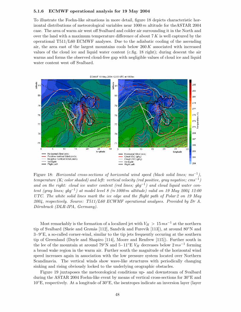
5.1.6 ECMWF operational analysis for 19 May 2004

To illustrate the Foehn-like situations in more detail, figure 18 depicts characteristic hor-izontal distributions of meteorological variables near 1000m altitude for theASTAR 2004case. The area of warm air west off Svalbard and colder air surrounding it in the North andover the land with a maximum temperature difference of about 7K is well captured by theoperational T511/L60 ECMWF analyses. Due to the adiabatic cooling of the ascendingair, the area east of the largest mountains cools below 260 K associated with increasedvalues of the cloud ice and liquid water content (c.fig. 18 right); during descent the airwarms and forms the observed cloud-free gap with negligible values of cloud ice and liquidwater content west off Svalbard.

Figure 18: Horizontal cross-sections of horizontal wind speed (black solid lines; ms−1),temperature (K; color shaded) and left: vertical velocity (red positive, gray negative; cms−1)and on the right: cloud ice water content (red lines; gkg−1) and cloud liquid water con-tent (gray lines; gkg−1) at model level 8 (≈ 1000m altitude) valid on 19 May 2004 12:00UTC. The white solid lines mark the ice edge and the flight path of Polar 2 on 19 May2004, respectively. Source: T511/L60 ECWMF operational analyses. Provided by Dr A.Dornbrack (DLR-IPA, Germany).

Most remarkably is the formation of a localized jet with VH > 15 ms−1 at the northerntip of Svalbard (Skeie and Grønas [112], Sandvik and Furevik [113]), at around 80◦N and3 - 9◦E, a so-called corner-wind, similar to the tip jets frequently occuring at the southerntip of Greenland (Doyle and Shapiro [114], Moore and Renfrew [115]). Further south inthe lee of the mountain at around 79◦N and 5 - 11◦E VH decreases below 2 ms−1 forminga broad wake region in the warm air. Further south the magnitude of the horizontal windspeed increases again in association with the low pressure system located over NorthernScandinavia. The vertical winds show wave-like structures with periodically changingsinking and rising obviously locked to the underlying orographic obstacles.

Figure 19 juxtaposes the meteorological conditions up- and downstream of Svalbardduring the ASTAR 2004 Foehn-like event by means of vertical cross-sections for 30◦E and10◦E, respectively. At a longitude of 30◦E, the isentropes indicate an inversion layer (layer

48

of increased thermal stability, i.e. denser contour lines) at about 500m altitude north of81◦N over the pack ice region. Towards south, the height of this capping inversion increasesup to 1000. . .1500 m altitude; south of 77◦N the tilted isentropes mark the baroclinic zoneassociated with the low pressure system further south. There, the magnitude of thehorizontal wind speed VH is maximum and amounts to about 22ms−1. Directly upstreamof Svalbard, VH ≈ 6 . . . 12 ms−1 depending on the altitude. Even the clouds visible inthe MODIS satellite imagery (c.fig. 11, left) are analysed by enhanced values of cloud iceand liquid water content upstream of Svalbard. The vertical wind speed at this upstreamsection is very low without any coherent structures.

Figure 19: Vertical cross-sections of vertical wind (color shaded; cms−1), horizontal windspeed (gray solid lines; ms−1, potential temperature (solid black lines; K) and cloud icewater content (white lines; gkg−1) and cloud liquid water content (blue lines; gkg−1) along10 ◦E (top) and 30 ◦E (bottom) valid on 19 May 2004 at 12:00 UTC. The gray areas belowthe absissas mark the locations of the pack ice up- and downstream of Svalbard, respectively.Source: T511/L60 ECMWF operational analyses. Provided by Dr A. Dornbrack (DLR-IPA, Germany).

In contrast, the vertical cross-section drawn downstream at 10◦E reveals pronouncedup- and downdrafts between 78◦N and 81◦N. The up- and downdrafts belong to twocounter-rotating horizontal vortex tubes with axes pointing into the plane plotted in fig-

49

ure 19: south of the ice edge, the northern vortex rotates anticlockwise and produces thestrong downdraft at about 79◦N in concert with its clockwise rotating counterpart furthersouth. Directly north of the downdraft in the center of the northern vortex tube, thehorizontal wind speed is maximum (VH ≈ 16 ms−1 at about 400m altitude) indicatingthe corner-wind or tip jet as seen in figure 18. It is interesting to note that the isentropicsurfaces in the vicinity of the ice edge are lifted significantly due to the upward motionand dropped due to the descending in the vortex. This results in a rather steep slopeof isentropic surfaces along the south-north flight pathes of the POLAR 2 on this day,c.fig. 18. Later, we will see that this characteristic shape of the isentropes and the associ-ated vertical transport of aerosols leads to a triangularly-shaped distribution of the lidarbackscatter ratio (c.cpt. 5.5).

The T511/L60 ECMWF operational analyses for 19 May 2004 was used as initialconditions for a high-resolution numerical experiment using the non-hydrostatic anelasticmodel EULAG (c.cpt. 5.9.2).

5.1.7 The mixed-phase cloud study of ASTAR 2004

In contrast to the clear-sky weather situations, the ASTAR 2004 measurements for thelow tropospheric mixed-phase clouds investigations were usually taken during periods ofpartly clear-sky, partly cloudy conditions (c.cpt. 5.10).

These conditions occurred predominantly at the end of the ASTAR 2004 campaign.Observations of mixed-phase clouds containing ice crystals during May/June are ratherunlikely at lower latitudes as much higher temperatures generate a pure water clouds inlow troposphere. However, the statistic of the meteorological data over Svalbard showsa significant amount of clouds containing ice crystals occurring between April and June(Herber et al. [65]).

The particular study described in chapter 5.10 deals with the observation of the naturalfeeder-seeder phenomenon with the ice crystals precipitating to supercooled boundary layerstratocumulus clouds.

5.2 Intercomparison of AMALi and KARL lidars operated in the zenith-aiming ground based configuration

For two measurements taken with different lidars, at the same time, in the same way, andwith application of the same profile averaging in time and space, their signal statisticscan still differ significantly due to differences in the emitted laser power, the sizes of theused receiving telescopes (Matthias et al. [102]). The system intercomparison is crucial toassess their ability to obtain the same results when the same evaluation scheme is applied.

The AMALi and KARL intercomparison measurements were taken for both systemsoperated simultanously at 532nm in a zenith-aiming ground based configuration undertypical ’lidar-day’ clear-sky weather conditions on 15 June 2004 between 21:30-22:10 UTat the Koldewey Station in Ny-Alesund. The systems were placed 30 m apart, distantenough to ensure that each lidar’s laser beam and telescope field of view will not overlapthe other up to the tropopause. In such a configuration KARL’s data were recorded upto the tropopause and the AMALi’s data up to 7.5 km height.

The lidars were compared with respect to the backscatter ratio profiles retrieved forboth lidars using the same evaluation scheme. The backscater ratio profiles were calculatedusing the standard Klett-Fernald-Sasano approach (Klett [28], Klett [29], Fernald [105],Sasano et al. [116]). The calculation was done under the assumption of the height inde-pendent lidar ratio of 30 srad resulting in a maximum of a backscatter ratio about 1.54 at500 m above ground. The KARL’s profiles were calibrated by setting a boundary condi-tion in the tropopause with backscatter ratio of 1.05. The AMALi profiles were obtained

50

up to 5.5 km and therefore calibrated at a height between 4.8 - 5.0 km with a backscatterratio of 1.06.

In figure 20 the temporal evolution of the backscatter ratio profiles of both lidarsobtained on 15 June 2004 between 21:30-22:10 UT (left and middle), as well as the 20minintegrated time intervals comparison at 21:30 UT and 21:50 UT with the profiles calculatedfor the entire time interval are presented.

The agreement of KARL and AMALi retrievals is very good with deviations less than3 %. Stronger deviations, up to 30%, are seen only at the range below 750m. There thelower, underestimated KARL’s backscatter ratios occur due to the wrong adjustment ofthe near-range small telescope on that particular day. Generally, the confidence in theKARL’s results obtained in the lowest 1.2 km frequently fails due to the difficulty of theassessment whether the proper adjustment of the near-range small telescope was made(Ritter [80]). The existence of an additional measurement providing cross-check valuesfor the Karl’s retrieval within the lowest troposphere could greatly improve the confidencein the results. An idea of a method with a potential of such validation using a scanningapproach with addittional lidar system (AMALi) is presented in chapter 5.3.

Figure 20: The comparison of the 532nm backscatter ratio profiles retrieved from measure-ments between 21:30-22:10 UT on 15 June 2004 for AMALi and KARL lidars operated inzenith-looking ground based configuration. Subvisible clouds passing the lidar site between1.5 - 1.8 km are well captured.

Deviations in the backscatter values at a layer between 1.4 km and 2.4 km altitude arecaused by passing thin, subvisible clouds, well captured by both lidars. Already for 20minintegration time both lidar retrievals converge, i.e. deviations in this height interval aremainly due to the high temporal and spatial variability of these clouds. The condensationin this layer must be dominated by small scale processes with a life time of 20min sincethe avaraging of the lidar signals is just sufficient to smear them out.

Good agreement of the profiles above the mentioned KARL’s lower range give evi-dence that both lidars obtain the same results. Whereby signals noise and/or detection

51

efficiencies of both instruments are of no concern, giving confidence for the future two-stream evaluation of the data obtained with lidars operated in airborne and groundbasedconfiguration (c.cpt. 5.4).

5.3 Variability of the particle extinction coefficient over the Kongsfjordobtained from the horizontally-aiming ground based AMALi mea-surements

On the 13.06.04 a one hour horizontal measurement with the AMALi lidar operating in theground based configuration from the NDSC Koldewey Station building was made to obtainthe particle extinction coefficient at 532 nm in the boundary layer over Kongsfjorden. Thelaser beam was sent at a small inclination angle of +2.5◦ from a height of 10m a.g. aiminginto the direction of uninhabitated area of the Tre Kroner mountain to avoide the potentialdanger with respect to the eye-safety.

This almost horizontal measurement allowed for the direct retrieval of the particle ex-tinction coefficient under the assumption of a homogeneous aerosol rich atmosphere usingthe slope method described in the chapter 4.3.1. The ’aerosol rich’ atmosphere assumptionmade usually for the horizontal measurements in the boundary layer at lower latitudes,i.e. αmol � αpart is not applicable in the case of relatively clear Arctic air. Hence, theextinction values obtained with the slope method have to be corrected for the contributiondue to the molecules. For this analysis, the molecular extinction coefficient αmol was cal-culated for the standard atmosphere with ps = 1013, 25 hPa and Ts = 288, 15 K resultingin a value of 2 · 10−5m−1.

The slope method applied to a period between 20:00 - 20:50 on 13.06.04 provided 5particle extinction coefficients averaged over 10 min at a range between 1150 - 1450 m:

Time [UT] 20:00 20:10 20:20 20:30 20:40αpart

532 [m−1] 3.29 · 10−5 3.12 · 10−5 4.45 · 10−5 8.94 · 10−5 4.63 · 10−5

Δαpart532 [m−1] ±0.18 · 10−5 ±0.26 · 10−5 ±0.16 · 10−5 ±0.19 · 10−5 ±0.26 · 10−5

These values correspond to a horizontal visibility of 10 - 20 km. The mean value of theparticle extinction coefficient amounts to 6.3 (±0.2) · 10−5m−1, averaged over the wholeperiod of 50min and in the same range. Within the given errors almost the same value ofthe particle extinction was obtained during the first 20min of the measurement. After-wards, a significant increase of the extinction is recorded. This indicates the short-termvariability of the particle optical properties on that particular day.

The knowledge of these extinction values can be of a great help for the correction ofthe KARL’s retrievals suffering from the high uncertainty in the lowest 1.2 km (c.cpt. 5.2).

In addition to the KARL’s measurements of particle extinction coefficient, the sun-photometer measurements of the optical depth of the whole atmosphere taken from theNDSC Koldewey Station building, as well as the in-situ measurements of the particle ex-tinction at the Zeppelin Mountain Station located about 1 km south of the NDSC buildingat about 500m altitude were available. Since these measurements are not directly com-parable another approach for the KARL’s validation is required.

From the AMALi particle extinction coefficients obtained with the slope approach theparticle backscatter coefficients can be calculated by applying the same lidar ratio valuethat was used for KARL’s particle backscatter coefficient profiles retrieved for each 10 minperiod. Hence, the values obtained with both lidars can be directly compared and theKARL’s profile can be corrected to match the AMALi validation values. Unfortunately,the simultaneous vertical measurements with KARL on that day were not possible due tothe occurrence of thick clouds at about 1.9 km altitude.

52

However, the idea of applying a small scanning lidar for validating the KARL’s re-trievals shall be used in the future, i.e. the combination with the AMALi’s scanningmeasurements taken from the Zeppelin Station with the laser beam sent every 60 s atone of the 3 angles of ± 20◦ and 0◦ providing (after slope inversion) for each time step 3particle extinction coefficients values at approximately 160m, 500 m and 860m and at therange between 1100 - 1500 m off the lidar. The values obtained at the two higher altitudeswill be used for the validation of the KARL’s profiles, and the value at the lowest altitudefor the interpolation of the KARL’s profiles down to the ground. Additionally, these mea-surements will allow the study of the extinction variability over the Kongsfjorden, also inthe case when thick clouds above 1000 m disable the KARL’s observations.

5.4 The two-stream inversion of the airborne nadir-aiming AMALi andzenith-aiming ground based KARL data

In this chapter the successfull and, to my knowledge, first-ever application of the two-stream backscatter lidar evaluation method to the non-simulated, real nadir-aiming air-borne and zenith-aiming ground based lidar signals is presented (Stachlewska et al. [33]).

The two-stream algorithm is revised, expanded and applied to data obtained duringsimultaneous measurements taken with a nadir-aiming AMALi, integrated onboard AWIresearch aircraft Polar 2, overflying a zenith-aiming KARL based in Ny-Alesund on Sval-bard during ASTAR and SVALEX campaigns. The feasability of the two-stream methodto retrieve extinction and backscatter coefficients profiles without assumption of their pro-portionality is demonstrated. The estimation of lidar constants is given in chapter 5.4.1.The comparison of the two-stream and Raman retrievals is presented in chapter 5.4.3. Thisproves the greater sensitivity and underlines the potential of the two-stream approach forspaceborne lidar data evaluation and validation during future ASTAR campaigns.

5.4.1 Estimation of the AMALi and KARL instrumental constants

The extinction coefficient profiles in the two-stream approach can be obtained directlywithout any a priori assumptions from the background and range corrected AMALi andKARL signals. However, to derive the backscatter coefficient profiles directly from thetwo-stream approach the instrumental constants have to be obtained first (c.cpt. 4.5.1).The method for the determination of the constants of ground based CK and airborneCA lidars, in case when one of the lidars observes an aerosol poor layer, as for examplein the free-troposphere, was proposed in chapter 4.5.2. Using this approach the KARLinstrumental constant CK was calculated from the β and α retrieved with Klett-Fernald’selastic KARL algorithm according to the constrains given in chapter 4.3.3.

Depending on assumed B(h) between the ground and the tropopause or the bottom ofCirrus clouds at about 8 - 9 km and selected boundary condition β(hr) at the calibrationinterval between 10 - 12 km an integration towards the aircraft’s flight level accumulatesto at least 20 % uncertainty of βpart(hf ). Different combinations of B(h) and β(hr) alterthe value of CK significantly less than the value of βpart(hf ) diminishing this uncertaintyby almost a factor of 4 if the mean of CK is calculated in the tropopause accordingto equation (30). For the data of 15 May 2004 best agreement of the optical depthobtained from the Klett-Fernald’s elastic KARL retrieval with both τpart

layer and τpartsun was

obtained for a boundary condition of βpartref = 0.3 (±0.05)·βmol resulting in a lidar constant

CK = 1.65 (±0.1) · 1014mV m3srad calculated at the mentioned calibration interval. Forthe same boundary condition CK = 2.03 (±0.1)·1014mV m3srad was found for the data of19 May 2004. The 23 % deviation in these values is due to the lower laser power caused byhigher surrounding temperature on the first day under investigation. The lidar constantfor the AMALi instrument was found to be CA = 1.43 (±0.1) · 1013mV m3srad.

53

5.4.2 Calculation constrains and errors of the two-stream AMALi and KARLretrievals

The two-stream calculation constrainsThe applicability of the two-stream method depends critically on the constraint that

both lidars probe the same air masses. Due to their relative movement AMALi and KARLdetected different air masses directly above the Koldewey Station and below the Polar 2aircraft. Hence, for the two-stream calculations of the βpart, αpart and B(h) profiles atthe heights directly above the lidar and directly below the aircraft more height steps thanrequired by constraints of geometrical compression of each lidar (c.cpt. 3.1 and 3.2.2) wereexcluded.

The data were pre-selected to obtain as high as possible signal-to-noise ratio of bothaverged signals whereby the spatial averaging of AMALi and temporal averaging of KARL’ssignals are kept as short as possible. Additionally, the clouds screening by interpolationof the signal values between the bottom and the top of the cloud, is applied in case whenany low density subvisible clouds were recorded by one of the lidars.

The extinction profiles on both days were derived directly from equation (4) using532 nm channel lidar signals provided with 60m range resolution, averaged over 10minin case of KARL and over 8min case of AMALi. The Poisson smoothing on 5 elementsis applied to the obtained extinction profiles. Both τlayer and τpart

layer in the range wherethe method was applied were calculated from these extinction profiles. The Rayleighextinction αmol and backscatter βmol profiles were obtained from radiosonde launches atthe Koldewey Station. The absorption contribution to the extinction, mostly due to theozone, shows negligible values at 532nm in the Arctic troposphere and was for this analysisneglected. Cirrus and subvisible clouds, if detected by KARL in the upper troposphere,were treated with low lidar ratios BCi = 12 for green light (Ansmann [96]).

An information on the particle optical depth of the whole atmosphere τpartsun was ob-

tained from sunphotometer measurements at the Koldewey Station. The zenith lookingKARL and the sunphotometer generally probe different air, i.e. sunphotometer measuresat 29◦ elevation above horizon and KARL underestimates retrieved values at the heightsbelow its geometrical compression. Therefore, the τpart

sun is used as a rough informationwhen compared with the particle optical depth obtained from the Klett’s elastic KARLretrieval. The values of CK and CA obtained in chapter 5.4.1 were used for the calculationsfor each day, respectively.

The two-stream contra the Raman retrievals - error comparisonThe two-stream 532 nm βpart, αpart and B(h) profiles were compared with correspond-

ing profiles derived from the Raman nitrogen KARL’s returns using Ansmann’s approach(Ansmann [96]). The Raman α profiles were derived from the inelastic scattering lidarequation for 607nm, while Raman β profiles were calculated from the ratio of 532nm and607 nm, both with the boundary condition βpart

ref derived in chapter 5.4.1 for consistency.The Raman evaluation was performed with a 20 minute integration time, i.e. twice aslarge as the integration intervals applied for the the two-stream retrieval. Further low-ering of the integration time of the Raman retrieval was not possible due to insufficientsignal-to-noise ratio of the averaged signals.

The errors of both types of the extinction retrievals depend almost entierly on thenoise of the signals. The main problem of the Raman extinction retrieval occurrs dueto the derivative of the noisy signal with height (Whiteman [117], Rocadenbosch [118].The calculations of the biases in the particle backscatter and extinction retrievals due tothe temperature dependence of the Raman scattering (Whiteman [119]) show negligablevalues for KARL’s nitrogen channel. In the case of two-stream extinction retrieval theerror is mainly due to the division of two noisy lidar signals. Hence, for the both types of

54

retrievals error propagation calculation was necessary.

According to error propagation the uncertainties of extinction coefficient (σext) andbackscatter coefficient (σbsc) retrieved with the Raman approach are σR

ext = 5 · 10−5m−1

and σRbsc = 1 · 10−7m−1srad−1.

The uncertainty of the two-stream extinction coefficient is σTSext = 1 · 10−6m−1. The

error of the two-stream backscatter is proportional to the error of lidar constants, i.e.the 5 % imprecision of the CK results in accuracy of the backscatter coefficient of σTS

bsc =1.5·10−7m−1srad−1. The noise of lidar signals and error of the determination of extinctionhardly affects the backscatter accuracy.

5.4.3 Comparison of the two-stream AMALi and KARL retrieval to the Ra-man KARL retrieval

The comparison of the retrievals obtained with the two different methods for the datataken on two days during the ASTAR 2004 campaign is discussed below.

For 15 May 2004 data recorded around 10:00 UT in a height layer between 635m and2435 m proved analysable. The cloud screening was applied to AMALi data in a layerof 120 m thickness around 1440m altitude. The two-stream βpart, αpart and B(h) (solidlines) compared to the corresponding values according to Ansmann’s Raman evaluation(dashed lines) are presented in figure 21 (red). The aerosol layer visible in the two-streamαpart retrieval with a maximum at 1800m altitude has its maximum at a 100 m loweraltitude in the Raman αpart profile. The lower aerosol layer has a maximum at around900 m altitude for both types of αpart retrieval but with higher values in the two-streamprofile. The total optical depth calculated for the two-stream layer τlayer sums up to aconsiderable value of 0.084, where particle optical depth τpart

layer is 0.064, mainly due tocontribution from both mentioned layers. Otherwise, the background particle extinctioncoefficient is around 0.15·10−4m−1, the background particle backscatter coefficient around0.7 · 10−6m−1srad−1 and a lidar ratio of 20 srad. These values are characteristic for theclean arctic summertime condition.

The profiles retrieved from the data recorded on 19 May 2004 at around 9:35 UT ata height interval between 815m and 2075m are shown in figure 21 (black). The cloudscreening of AMALi data in a layer of 120m thickness around 1020m altitude was nec-essary. At the altitude of around 1800m a layer of enhanced extinction and lidar ratio isvisible again. Apart from this layer the air appears clean with similar particle extinctionbackground value and lidar ratio as for the previous day and τlayer of 0.035 and τpart

layer

of 0.02, mainly due to mentioned aerosol layer. For this day even lower values of thebackground particle backscatter coefficient around 0.3 · 10−6m−1srad−1 were observed.

The retrievals of the two-stream and the Raman techniques on both days agree well.Given mentioned uncertainties of extinction and backscatter coefficients σTS and σR allretrieved βpart, αpart and B(h) profiles coincide well, with small deviations only in thelayers of highest extinction values. While for 15 May 2004 one might speculate about aslight height shift between the profiles, such a behaviour is not observed on the secondday. Therefore, we address these deviations partially to noise, with above given errortolerances, and partially to real variations of the atmosphere during the longer intergrationof the Raman-shifted lidar profiles (c.cpt. 5.4.2).

For both days layers of enhanced extinction values hardly visible in the backscatterprofiles were observed, underlining the necessity to determine backscatter and extinctionindependently of each other from the lidar measurements (Sasano [116]). The discussionof the physical origin of these layers is given in chpater 5.8.

55

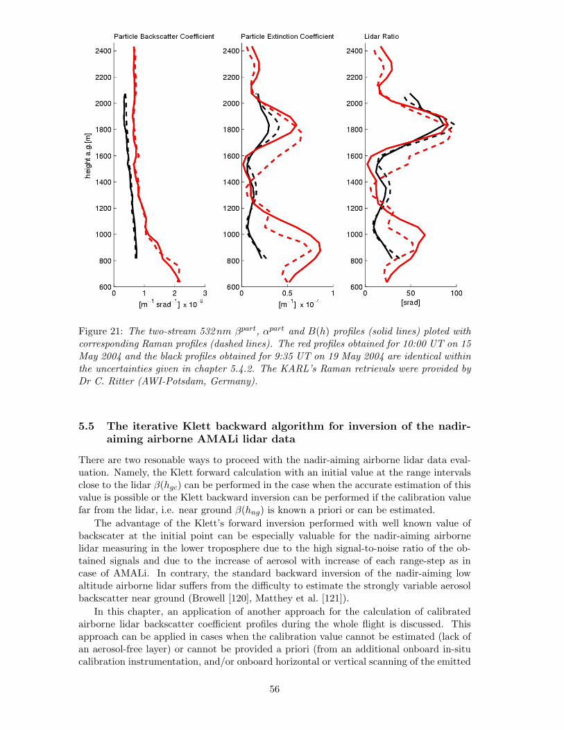
Figure 21: The two-stream 532nm βpart, αpart and B(h) profiles (solid lines) ploted withcorresponding Raman profiles (dashed lines). The red profiles obtained for 10:00 UT on 15May 2004 and the black profiles obtained for 9:35 UT on 19 May 2004 are identical withinthe uncertainties given in chapter 5.4.2. The KARL’s Raman retrievals were provided byDr C. Ritter (AWI-Potsdam, Germany).

5.5 The iterative Klett backward algorithm for inversion of the nadir-aiming airborne AMALi lidar data

There are two resonable ways to proceed with the nadir-aiming airborne lidar data eval-uation. Namely, the Klett forward calculation with an initial value at the range intervalsclose to the lidar β(hgc) can be performed in the case when the accurate estimation of thisvalue is possible or the Klett backward inversion can be performed if the calibration valuefar from the lidar, i.e. near ground β(hng) is known a priori or can be estimated.

The advantage of the Klett’s forward inversion performed with well known value ofbackscater at the initial point can be especially valuable for the nadir-aiming airbornelidar measuring in the lower troposphere due to the high signal-to-noise ratio of the ob-tained signals and due to the increase of aerosol with increase of each range-step as incase of AMALi. In contrary, the standard backward inversion of the nadir-aiming lowaltitude airborne lidar suffers from the difficulty to estimate the strongly variable aerosolbackscatter near ground (Browell [120], Matthey et al. [121]).

In this chapter, an application of another approach for the calculation of calibratedairborne lidar backscatter coefficient profiles during the whole flight is discussed. Thisapproach can be applied in cases when the calibration value cannot be estimated (lack ofan aerosol-free layer) or cannot be provided a priori (from an additional onboard in-situcalibration instrumentation, and/or onboard horizontal or vertical scanning of the emitted

56

lidar light is not available).The trick to get rid of this calibration problem is, as proposed in chapter 4.6, to estimate

accurately the value of backscatter at a range close to the lidar β(hgc) and to perform theKlett’s backward inversion in an iterative way. The calculation of calibrated airbornelidar backscatter ratio profiles is performed in the following steps. Firstly, calculate theparticle backscatter value βpart(hgc) close to the aircraft under the assumption that thetransmittance term T = 1 near the aircraft; secondly, guess the βpart

Klett(hng) near groundand use it as a calibration value for the calculation of the particle backscatter profileusing the backward Klett inversion; thirdly, check whether the calculated value of thebackscatter at the height close to the aircraft βpart

Klett(hf ) matches the estimated βpart(hgc);if not, change the value of βpart

Klett(hng) accordingly to Newton method, recalculate theβpart

Klett(h) profile and compare both values again; finally, perform such iterations untilβpart

Klett(hf ) and βpart(hgc) match.In this thesis few examples of the application of this iterative approach with respect

to the study of the different types of aerosol (c.cpt. 5.9.1) or in the case study of the lowdensity mixed-phase clouds (c.cpt. 5.10) are discussed. In chapter 5.5.2 an example of suchcalculations for the airborne AMALi measurements obtained under a clear-sky conditionsin the gap area as described in chapter 5.1 is presented.

5.5.1 The discussion of the uncertainties of the iterative airborne inversion

Unlike for the zenith-looking tropospheric lidars (Masumoto and Takeuchi [122]), generally,for the short-range nadir-aiming airborne lidar the largest term of the error propagationof the backscatter coefficient profiles is due to the wrong assumption/estimation of thebackscatter calibration value (partial derivative of backscatter over range). The wrongassumption of the lidar ratio contributes much less to the backscatter ratio uncertainty(small partial derivative of backscatter over lidar ratio).

In the case of the approach proposed in this thesis the assumption of the transmittanceterm T = 1 in the airborne lidar equation permits accurate estimation of β(hgc) in rangeintervals close to the lidar, i.e. at an altitude near the aircraft but beyond geometricalcompression of the lidar (c.cpt. 4.6).

In case of the AMALi lidar, for the height chosen just below a geometrical compressionof 235m the expected error for neglecting the transmittance term varies from 0.7 % for theparticle extinction of 0.15 · 10−4m−1 typical for clear Arctic atmosphere (T ≈ 0.993), upto 2.8 % for the particle extinction of 0.6 · 10−4m−1 for aerosol contaminated atmosphere(T ≈ 0.972). Hence, the clearer the atmosphere and the better the knowlegde of themolecular contribution to the extinction αmol (for example from nearby meteorologicalsounding) the better the transmittance estimate, i.e. the lower uncertainty of the β(hgc)calculation.

Hence, the accuracy of the α and β calculated with the iterative approach at any timeduring the flight depends mainly on the assumption of the lidar ratio since the error ofthe estimation of β(hgc) near the aircraft (and dependent on it, iteratively found β(hng)near ground) hardly affects the error of the backscatter retrieval itself.

5.5.2 The application of the iterative airborne inversion for the calibrated’along-flight’ backscatter coefficient calculation

The lidar backscatter ratio profiles obtained during the whole flight on 19 May 2004 and21 May 2004 are shown in figure 22. Both flights were performed under similar weatherconditions (c.cpt 5.1) and show similar values of the retrieved backscatter ratios. Hence,for brevity only results for the first day are discussed in detail in the following. Mind, thatthe corresponding flight path for that day was sketched in figure 18.

57

Figure 22: The calibrated backscatter ratio profiles along the flight (c.fig.4 and 18) retrievedusing the iterative Klett’s approach for 19 May 2004 (top) and 21 May 2004 (bottom). Thedata were obtained by the nadir-aiming airborne AMALi lidar from the flight altitude of2650m and from 3000m, respectively, during the ASTAR campaign.

58

On 19 May 2004, the measurements started just after leaving the base at Longyerbyenairport. Firstly, the heading in the direction of Ny-Alesund to overfly the stationaryKARL lidar at the Koldewey Station was taken. Afterwards, the heading North-Westcontinued until the cloud band above the ice edge was reached. Then the Polar 2 turnedto South-West direction and continued along a strait path down to Bellsund mouth area.Finally, after turning offshore Wedelland plain the heading West was taken and at thelatitude of Isfjord mouth changed to heading East in direction of Longyearbyen.

The simultaneous measurements of AMALi and KARL taken during the Koldewey Sta-tion overflights allowed to obtain the AMALi lidar instrumental constant CA = 1.43 (±0.1)·1013mV m3srad (c.cpt. 5.4.1) which was used in the two-stream inversion (c.cpt. 5.4.3).The obtained lidar ratio profile at the Ny-Alesund location showed mainly background li-dar ratio of 20 srad with a layer of extremally high values of the lidar ratio of 80 srad dueto the existence of the aerosol layer of rather local origin (c.cpt. 5.8). Additionally, the airmass transport had an non-uniform character, whereby a contamination with the anthro-pogenic aerosol could not be totally excluded (c.cpt. 5.1.4 and 5.1.5). Hence, the choiceof the appropriate lidar ratio for calculations along the flight was not straight forward.

Therefore, the sensitivity study with respect to the estimation of the error due to theassumption of a different type of lidar ratio were performed. For the following constraintson the lidar ratio the error of the backscatter coefficient calculation was obtained:

B(h) = const [srad] 20 25 30 35

Δβpartt1 [m−1srad−1] ±1.8 · 10−7 ±0.3 · 10−7 ±0.7 · 10−7 ±1.4 · 10−7

assumed for the clean air, the clean air with a bit of aerosol, the air with considerableaerosol load, and the polluted arctic air, respectively. Additionally, the height dependentlidar ratio set to 35 srad between 0 - 1600 m and to 20 srad at 1600 - 2500 m were performedfor which (within the given above uncertainties) the same values of the particle backscattercoefficients as for the corresponding constant lidar ratios results were obtained.

Hence, the sensitivity studies show no significant hindering of the iterative calculationswhen the constant lidar ratio is assumed. This result is mainly due to the short integrationrange for the AMALi measurements, so that the assumption of the constant lidar ratiodoes not introduce significant error, as discussed in chapter 5.5.1. The accuracy of thebackscatter coefficient calculated with the iterative approach is assumed to be σIK

bsc =2.0 · 10−7m−1srad−1.

The backscatter ratio profiles (c.fig. 22) were calculated with 15 s temporal resolutioncorresponding to 1 km spatial resolution to provide appropriate tamporal and spatial res-olution for the comparisons with the ECMWF operational analyses (c.cpt. 5.1) and theEULAG model results (c.cpt. 5.9.2). In case of thick clouds the backscatter ratio couldnot be retrieved due to the multiple scattering.

The striking feature captured on both backscatter ratio plots are the triangularly-shaped aerosol gradients measured in the North-West area offshore Svalbard. In bothcases, the flight paths were nearly parallel to this aerosol gradients at the northernmostpart of the flights. It is interesting to note that the triangular shape of the aerosol distri-bution is probably related to the vertically rised isentropic surfaces (c.fig. 19, top). Thus,the enhanced vertical transport of the sea salt aersosls from the rough sea in the region ofthe corner-wind is most likely responsible for high aerosol load inside the ’triangles’. Thisis studied in detail in chapter 5.9.2 by using a high resolution numerical model EULAGfor the emission and transport of different aerosol types. For example, this analysis al-lowed for the interpretation of the very high backscatter ratios in the lowest altitudes atthe end of the flight observed just outside the Isfjorden mouth by associating it with theAdventalen dust event which occured a day before (c.cpt. 5.9).

59

5.6 Clean and polluted Arctic air and their characteristic properties

The airborne missions of ASTAR 2004 focused on investigation of horizontal and verticalextend, layering and characteristics of tropospheric aerosol of typical clean Arctic summerconditions protected from a long-range transport of polluted air masses. A similar studybut for the aerosol loads contaminated with the anthropogenic origin particles advectedto the Arctic from the lower latitudes was in focus of the SVALEX 2005.

The fact that the lidar measurements during both ASTAR and SVALEX where takenin the similar conditions (stable Foehn-like conditions) and in the same area of interest(overflying the Koldewey Station in Ny-Alesund), allowed for the direct comparision of thelidar retrievals from both campaigns (c.cpt. 5.1). During ASTAR Foehn-like period onlyfew AMALi overflights were performed due to the partly cloudy conditions just over theKoldewey Station. During SVALEX three days of non-stop measurements with KARL,the longest measurement period at a time in its history, with 13 AMALi overflights coveredthe entire Foehn-like period.

Here the results of the comparison study with respect to measurements taken on 19May 2004 and 14 April 2005 are presented. The first of the selected for the two-streamretrieval profiles represents the background aerosol loads of clean conditions investigatedduring the Foehn-like period between 18 - 23 May 2004. The second profile, with muchhigher aerosol load, is representative for the Arctic Haze event which occured during 12-16April 2005 Foehn-like period.

The optical properties of investigated atmosphere on each of this days were obtainedusing the two-stream approach. The two-stream βpart, αpart and B(h) profiles obtainedfor both days at 532nm were derived with the constraints described in chapter 5.4.3. Thecloud screening for the SVALEX day was not necessary. The values of CK = 2.03 (±0.1) ·1014mV m3srad and CA = 1.43 (±0.1) · 1013mV m3srad and a boundary condition ofβpart

ref = 0.3 (±0.05) · βmol were used for the calculations for both days. The uncertaintyof the retrieved two-stream extinction σTS

ext is 1 · 10−6m−1 and the error of the two-streambackscatter σTS

bsc is 1.5 · 10−7m−1srad−1.Sets of profiles αpart(h), βpart(h), and B(h) obtained for each day are presented in fig-

ure 25. These profiles were compared between each other and interpreted in terms of theiroptical properties (extinction, backscatter, depolarisation, optical depth), macrophysicalproperties (humidity, temperature, origin) and microphysical parameters (refractive in-dex, size distribution and particle number concentration) providing ’clean’ contra ’haze’characteristics (c.cpt. 5.6.2 and 5.6.3, respectively).

5.6.1 General situation during ASTAR 2004 and SVALEX 2005

General situation during ASTAR 2004The preliminary analysis of all of the aerosol airborne in-situ measurements taken

from onboard the Polar 4 aircraft during the whole ASTAR 2004 campaign (Matsuki etal. [123]) confirmed the typical clean Arctic background conditions characterised by lowvalues of aerosol concentrations and extinctions and low variability throughout the wholetroposphere (c.fig. 23).

However, during some flights distinct differences between different layers in the free tro-posphere were found, both for accumulation mode aerosol and fine particles. On some daysan intensive new particle formation in marine boundary layer near Ny-Alesund reachingaerosol number concentration up to 3 - 4·103ppcm−3 were observed. On the flights per-formed in centre of low pressure system were it was measured very clean air mass withalmost completely depleted accumulation mode aerosol and relatively high total num-ber concentrations ranging from 5 - 10·102ppcm−3 in marine boundary layer and in freetroposphere.

60

Figure 23: The preliminary results of the aerosol in-situ measurements obtained from allPolar 4 flights justifying the clean Arctic background conditions during the ASTAR 2004campaign. Provided by A. Minikin (DLR-IPA, Germany).

The in-situ and remote ground-based measurements at the Koldewey, Rabben andZeppelin stations generally confirmed the airborne observations. Very clean conditionsmanifested in the low amounts of the light absorbing particles (soot) remaining below10 ng cm−3 for long periods. Particle number densities ranged from less than 200 to above1000 ppcm−3 with very low concentrations of large particles (less than few ppcm−3).

According to sunphotometer measurements taken in Ny-Alesund, only low aerosolcontaminations were observed. The daily average of the particle optical depths τpart

sun

retrieved for the 532nm was varying around 0.075 and 0.055 at the beginning and endof the ASTAR Foehn-like period (c.fig. 24). The low values of the Angstrom exponentsugests that the values of τpart

sun must be, at least partially, addressed to the existence ofthe passing subvisible clouds or Cirrus (Sassen and Arnott [124]).

Figure 24: The comparison of the daily averaged particle optical depth spectra obtainedwith the sunphotomether during the Foehn-like period at ASTAR (dashed redish curves)and SVALEX campaigns (solid blueish). The sumphotometer data were provided by A.Herber (AWI Bremerhaven, Germany).

61

From KARL’s measurements, usually, background values of backscatter and extinc-tion coefficients with no depolarisation justifying the existence of only spherical particleswere retrived. For some days a humid layers of enhanced extinction, hardly visible in thebackscatter profiles, where obtained also from KARL’s Raman measurements (c.cpt. 5.8).Additionally, sometimes high values of volume depolarisation at 532nm below 2 km alti-tude were recorded, indicating elongated particles of ice crystals or diamond dust.

General situation during SVALEX 2005During the SVALEX Foehn-like period the daily average of the particle optical depths

derived from the sunphotometer data at 532nm varied between 0.065 and 0.12 (c.fig. 24).These high values address the haze aerosol, since no existence of Cirrus or subvisibleclouds in troposphere was observed, except for the 12 May 2005. The sunphotometer datawere corrected for the ozone contribution at the wavelengths within the ozon absorptionband (350 - 370nm and 450 - 800nm), i.e. in the case of the 533 nm detection channel thecorrection of the particle optical depth of about 0.02 for the 300 - 350DU .

Generally, KARL’s retrievals showed high particle extinction coefficient around 3 -4·10−5m−1 (form 607nm) and high particle backscatter coefficient 1 - 2.5·10−6m−1srad−1

(form 532nm/607 nm) with lidar ratios of around 35 srad, i.e. values characteristic for thepolluted arctic spring condition. Only low volumne depolarisation ratios at 532nm wererecorded. Also during the SVALEX at some days layers of strongly enhanced extinction,hardly visible in the backscatter profiles, where observed (c.cpt. 5.8).

5.6.2 Background aerosol load at ASTAR campaign

The two-stream profiles of the particle extinction coefficient, the particle backscatter co-efficients and corresponding lidar ratio obtained for 532nm on 19 May 2004 are presentedin figure 25 (dashed).

Figure 25: The two-stream βpart, αpart and B(h) profiles obtained for 532nm on 19 May2004 (dashed) ASTAR and 14 April 2005 (solid) SVALEX mesurements.

62

For data of 19 May 2004 recorded at around 9:35 UT a height interval between 815mand 2075m was analysed. The aerosol layer with a maximum at about 1800m altitudewith αpart enhanced up to 0.3 · 10−4m−1 and lidar ratio of 80 srad. Otherwise the air wasclean with typical for the Arctic background values of particle extinction of 0.15 ·10−4m−1,lidar ratio of 20 srad and very low values of particle backscatter increasing towards theground level in a range of 0.3 - 0.7·10−6m−1srad−1. The total optical depth calculatedfor the layer where the two-stream method was apapplied τlayer sums up to 0.035 withparticle optical depth τpart

layer of 0.02.The sunphotometer measurements in Ny-Alesund at 9:40 UT on that day recorded

τpartsun 0.107 for green light, partly contaminated by passing subvisible clouds at about the

flight altitude and Cirrus at 8 - 9 km, both detected also by KARL. However the high valueof the Angstrom exponent indicates the existence of small particles which might be dueto the aerosol contamination or the existence of a small water droplets (c.fig. 24).

The radiosonde ascent at 11:00 UT in Ny-Alesund (c.fig. 13, green) show general trendof increase of the relative humidity (from 58 % to 72 %) and decrease of the temperature(from −8 oC to −14 oC) with the height within the layer where the two-stream was applied.The temperature inversion at about 1800 m is evident (c.cpt. 5.8).

The inversion of the microphysical parameters of the profiles measured on 19 May2004 was not possible, since the condition of providing the set of at least 2 α and 3 βnecessary for the inversion (c.cpt. 4.7) was not fullfield, due to the failure of KARL’s355 nm detection channel. Therefore, inversion for the set of retrieved backscatter andextinction profiles obtained with KARL on 18 May 2004 is given in figure 26. As themeasured on that day background values of extinction and backscatter coefficients werein the order of magnitude of the ones measured on the 19 May 2004, as well as on otherclear-sky days during the campaign, the obtained results are considered as representativefor most measurements during ASTAR.

The values characteristic for the background conditions of the complex refractive in-dex m = 1.4 + 1 · 10−4 i typical for the water particles, the bimodal size distribution(Morawska et al. [125]) dominated with only a few large particles of the effective radiusvarying between 0.6 - 1.2 μm with very narrow σ of 1.26 and an extremally low particleconcentrations varying between 0.5 - 3 cm−3 were retrieved.

Generally, during most days of the ASTAR campaign, the NOAA HYSPLIT backwardtrajectories calculated for the Ny-Alesund location showed the air trapped at lower tropo-spheric layers in the high Arctic (c.cpt. 5.1.4). Although, for 19 May 2004 the NOAA HYS-PLIT backward trajectories (c.fig. 14) and the FLEXPART retroplum (see: Polar 2 time 1at http://zardoz.nilu.no/∼andreas/ASTAR/) show air masses passing through non-polarregions at a different locations for the various analysed altitudes. In addition the FLEX-PART indicated possible antropogenic pollution in-take over Finland and Kola Peninsulaat about 1800m, which is an altitude corresponding to the maximum extinction on thisday (c.fig. 25). However, the contamination with the anthropogenic pollution from thelower laltitudes seem not likely due to the very low extinction of these air mass. Therefore,the air measured on 19 May 2004 can be interpreted as a typical for the clean summerconditions in Arctic (d’Almeida et al. [126], Covert et al. [127], Zielinski and Patelski [58]),with a humid layer of local origin rather than of an advection phenomenon (c.cpt. 5.8).

5.6.3 Increased aerosol load at SVALEX campaign

For the measurements taken on 14 April 2005 at around 14:45 UT the analysed heightinterval between 700 m and 2500m show strongly enhanced βpart, αpart and B(h) in com-parison with the corresponding ASTAR profiles. The lowest values of the particle ex-tinction are around 0.3 · 10−4m−1 corresponding to the maximum of the measured valueson 19 May 2004. Likewise, the values of the backscatter are much higher then previously

63

varying between 0.9 - 2.2·10−6m−1srad−1. The lidar ratio varies around 35 srad indicatingpolluted Arctic atmosphere. The total optical depth of the two-stream layer τlayer sumsup to considerable 0.095 with the particle optical depth τpart

layer of 0.076.The sunphotometer measurements at 14:45 in Ny-Alesund for the green light recorded

τpartsun of 0.084 (c.fig. 24), while for the whole Foehn-like period mean value of 0.099 in

Ny-Alesund and of 1.19 in Longyerbyen was obtained, interpreted as high enough to beassociated with Arctic Haze particles (Heintzenberg [11]).

There is no evidence of Cirrus or subvisible clouds in upper troposphere from KARLmeasurements and both lidars show no depolarisation signature at 532nm.

Figure 26: The results of the microphysical parameter inversion obtained for the sets of theKARL’s αpart and βpart at 355 nm, 532 nm and 1064 nm. On 18 May 2004 and 14 April2005 retrieved values represent the characteristic clean (ASTAR) and polluted (SVALEX)conditions. On 15 May 2004 and 15 April 2005 calculations were done for the altitudescorresponding to the layers of strongly enhanced αpart undiscernible in βpart, independenton the clean/polluted conditions during both campaigns (c.cpt.5.8). The microphysicalparameter inversion code was provided by Dr C. Bockmann and A. Kirsche (Universityof Potsdam, Germany). The calculations were performed from the KARL’s measurementsby Dr C. Ritter (AWI-Potsdam, Germany).

The radiosonde ascent at 12:30 UT in Ny-Alesund recorded the mean value of relativehumidity of 31 % and temperature of −12.2◦C within the layer where the two-streamwas applied (c.fig. 13). The decrease of temperature and relative humidity droping from50 % at 700 m to its minimum of 22 % at about 2000m and rising again to reach 28 % at2500 m shows similarities with the particle extinction profile. Just below a weak inversionlayer seem to be present, otherwise there is no evidence of existence of inversions up to

64

tropopause.The inversion of the microphysical parameters for KARL’s measurements on 14 April

2005 retrieved the complex refractive index m = 1.68 + 3 · 10−3 i typical for anthro-pogenic aerosol (c.fig. 26). Slightly higher than usual value of Re m indicate possible sootcontamination, not unusual during the Arctic Haze events in this area (Yamanouchi etal. [19]). The size distribution is characterised by a monomodal log-normal distribution(Morawska et al. [125]) with the effective radius of 0.2 μm with σ of 1.7 and high particleconcentrations varying between 50 - 150 cm−3.

Both, the NOAA HYSPLIT and the FLEXPART analysis, indicate the uniform trans-port form Yenisey and Lena Delta where the soot particles can be expected as a source ofcontamination (c.cpt. 5.1.4 and 5.1.5). The local source of contaminations with CO, NO2

and SO2 are possible at Ny-Alesund area at 14:45.The measured enhanced values for the extinction and the backscatter coefficient with

almost constant but significantly higher than typical clean Arctic air lidar ratio values,the low humidity and volume depolarisation with the high particle concentrations togetherwith the trajectories justify anthropogenic contaminations. Especially the high extinctionof this air and long duration of its way through mid-continental area makes such con-taminations possible. Therefore, advection of anthropogenic origin air masses from themid-latitudes, i.e. the Arctic Haze event, seems more likely than any local contaminations.

5.7 Estimation of the temporal progress of the Arctic Haze event duringSVALEX campaign

In this chapter a study focused on the Arctic Haze temporal progress for the observationstaken on 15 April 2005 during the day of the strongly enhanced aerosol load in the vicinityof Ny-Alesund and Longyearbyen under the Foehn-like conditions during the SVALEXcampaign is presented. On that day sunphotometers in both mentioned sites recorded thehighest values of the particle optical depth, while generally higher values were measuredduring the whole campaign in Longyearbyen.

On 15 April 2005 between 11:46-13:04 UT AMALi flew 5 times over KARL. For brevityhere 3 of these overflights, first, third and fifth, refered to as t 1, t 3 and t 5, are analysedand interpreted.

The data obtained for each of these overflights are directly comparable, as each wasmade along the same flight path and against the wind direction blowing from the glacierlocated in south-eastern end of the fiord towards the mouth of the fiord. The flight turnpoints were done over an open sea outside the fiord and over a the Tre Kroner behind theglacier. The aircraft crusing speed was lowered to a minimum of 90 kt for each overflightwhich allowed to aquire highest possible number of laser-shots within the area of interestand to increase the representativity of the data collected with AMALi. Hence, the bestcompatibility of KARL signals averaged over time with AMALi signals averaged over timeand space was achieved.

The calculations of the sets of particle extinction and backscatter coefficient and thecorresponding lidar ratio profiles was done using the two-stream approach (c.cpt. 5.4and 4.5). In contrary to the standard two-stream approach where the backscatter ra-tio calibration value is set to unity at the range where both signals show the same shape(Cuesta [128]) in our case it is calculated for each of the times from equation 28 with thetransmittance term obtained from the two-stream extinction profiles for that particulartime and the lidar instrumental constants obtained according to chapter 4.5.2. Within thegiven uncertainties the values of both constants at 532nm were the same for each time in-terval, i.e. CK = 1.03 (±0.1)·1014mV m3srad and CA = 4.2 (±0.1)·1013mV m3srad. Theadvantage of this approach over the mentioned above standard approach is clear. Evenin very clean Arctic atmosphere, as during the ASTAR 2004, the background backscatter

65

ratio values ranges between 1.2 - 1.6 (c.fig. 20 and 30), i.e it is always highier than thevalue of the backscatter ratio due to the molecules alone, which is by definition unity.Hence, the standard approach results in bias in the backscatter ratio and the lidar ratioretrievals, while this approach not.

1 1.5 2 2.5 3 3.5 4 4.5 5 5.5

x 108

600

800

1000

1200

1400

1600

1800

2000

2200

2400

2600

Amali & Karl Pr2 Signals 050415 11:46−11:53−solid, 12:22−12:29−dashed, 12:57−13:04−dotted

signal strength

heig

ht a

.g.[m

]

Figure 27: The range and background corrected signals at 532 nm of AMALi (blue) andKARL (red) for time intervals t 1 (sloid), t 3 (dashed) and t 5 (dotted) obtained on 15 April2005 during the Arctic haze SVALEX measurements. The signals are investigated priorto the two-stream method application to pre-select the regions for the inversion.

The visual inspection the range and background corrected lidar signals (c.fig. 27) withina range of KARL’s and AMALI’s completed overlap (0.6 - 2.64 km) show significant differ-ences at particular altitudes where systems sampled into different air, i.e. for all profilesbetween 2.1 - 2.64 km directly below AMALi lidar and for t 3 profile at around 1.65 km.The visual assesment of the lowest range of the applicability of the method is not as straitforward, due to the strong increase of the KARL’s signal.

The range of the two-stream applicability was defined in a layer between 1.2 - 2.1 kmfor each profile (c.fig. 28). The optical properties retrieved for 532nm within this layerrange with the uncertainties obtained as in chapter 5.4.3 are given below:

profile αpartlayer [m−1] βpart

layer [m−1srad−1] Blayer [ srad] τpartlayer

t1 2.8 (±0.1) · 10−5 1.1 (±0.15) · 10−6 26 0.026t3 4.6 (±0.1) · 10−5 1.4 (±0.15) · 10−6 33 0.042t5 4.7 (±0.1) · 10−5 1.45 (±0.15) · 10−6 32 0.043

Each of the AMALi and KARL signals and the retrieved backscatter and extinctionprofiles show fast (within about an hour) increase for each overflight to the values typicalfor polluted arctic air (d’Almeida et al. [126]).

Interesting enough that below 1.2 km a layer of enhanced extinction and lidar ratio,similar to these found during the ASTAR measurements, is evident (c.cpt. 5.8).

66

Since overflights were performed in the same area, a contamination with the aircraft’sexhaust itself has to be taken into account. However, the visual observations of a decreaseof the visibility in Kongsfjord during these overflights linked it with an advection of thepollution from the direction of Longyearbyen (Stachlewska [79]). Both, the long-rangetransport of the continental pollutants, as well as contaminations of a local origin cannotbe excluded. Two possible scenarios can explain the obtained optical parameters, anadvection of particles of the same composition and microphysical properties but larger insize at each time or/and an advection of particles of the same size and composition whichstart to grow in Kongsfjord.

−2 0 2

x 10−4

600

800

1000

1200

1400

1600

1800

2000

2200

2400

2600

[m−1]

heig

ht a

.g.[m

]

0 2 4

x 10−6

600

800

1000

1200

1400

1600

1800

2000

2200

2400

2600

Two−stream Retrievals 050415 at 11:46−11:53−solid, 12:22−12:29−dashed, 12:57−13:04−dotted [UT]

[m−1srad−1]

−100 0 100600

800

1000

1200

1400

1600

1800

2000

2200

2400

2600

[srad]

Figure 28: The two-stream 532nm βpart, αpart and B(h) profiles for time intervals t 1(sloid), t 3 (dashed) and t 5 (dotted) retrieved for 15 April 2005 during the Arctic HazeSVALEX measurements. At about 1200m a layer of strongly enhanced particle extinctioncoefficient is evident. The negative values at about 1700m (t 3) and at 2200m (t 3 and t 5)are caused by lidars sampling into different air masses (c.fig.26).

This study demonstrates a great advantage of the two-stream method over the Ra-man method for observations of the temporal development of the small-scale atmosphericevents. The typical day-time KARL’s Raman extinction profile has a resolution of 1 - 3h(c.cpt. 3.1). In special cases the resolution of such retrievals can be improved to 20 min(c.cpt. 5.4.3). However, in this latter case the evaluation is very difficult due to significantlylarge noise of the Raman signals and, hence the strong dependence of these retrievals onapplied smoothing.

Lowering of the crusing speed of the Polar 2 aircraft to the minimum (90 kt) allows forprolongation of the sampling time of ’the same’ air mass by both lidars during the AMALi’soverflights. Hence, the two-stream retrievals with 8 - 10 min averaging are provided. Suchadjustment of the speed of the CALIPSO satellite during the future CALIPSO lidar andKARL lidar validation experiments will not be possible.

Therefore, during the next ASTAR campaign the measurements in an extra mode,namely the zenith-aiming airborne AMALi and the CALIPSO lidar, shall be performed to

67

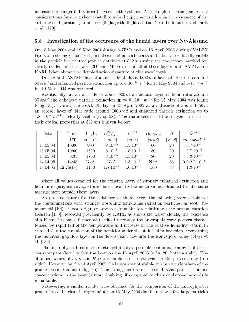
increase the compatibility area between both systems. An example of basic geometricalconsiderations for any airborne-satellite hybrid experiments allowing the assesment of theairborne configuration parameters (flight path, flight altutude) can be found in Gebhardtet al. [129].

5.8 Investigation of the occurence of the humid layers over Ny-Alesund

On 15 May 2004 and 19 May 2004 during ASTAR and on 15 April 2005 during SVALEXlayers of a strongly increased particle extinction coefficients and lidar ratios, hardly visiblein the particle backscatter profiles obtained at 532nm using the two-stream method areclearly evident in the lowest 2000m. Moreover, for all of these layers both AMALi andKARL lidars showed no depolarisation signature at this wavelength.

During both ASTAR days at an altitude of about 1800m a layer of lidar ratio around80 srad and enhanced particle extinction up to 6·10−5m−1 for 15 May 2004 and 3·10−5m−1

for 19 May 2004 was retrievedAdditionally, at an altitude of about 900m an aerosol layer of lidar ratio around

60 srad and enhanced particle extinction up to 8 · 10−5m−1 for 15 May 2004 was found(c.fig. 21). During the SVALEX day on 15 April 2005 at an altitude of about 1150man aerosol layer of lidar ratio around 100 srad and enhanced particle extinction up to1.8 · 10−4m−1 is clearly visible (c.fig. 28). The characteristic of these layers in terms oftheir optical properties at 532nm is given below:

Date Time Height αpartin layer αpart Bin layer B βpart

[UT] [m a.s.l.] [m−1] [m−1] [srad] [srad] [m−1srad−1]15.05.04 10:00 900 8·10−5 1.5·10−5 60 20 0.7·10−6

15.05.04 10:00 1800 6·10−5 1.5·10−5 80 20 0.7·10−6

19.05.04 9:35 1800 3·10−5 1.5·10−5 80 20 0.3·10−6

14.04.05 14:45 N/A N/A 3-8·10−5 N/A 35 0.9-2.2·10−6

15.04.05 12:25(t3) 1150 1.8·10−4 4.6·10−5 100 33 1.3·10−6

where all values obtained for the existing layers of strongly enhanced extinction andlidar ratio (asigned in layer) are shown next to the mean values obtained for the samemeasurement outside these layers.

As possible causes for the existence of these layers the following were considerd:the contaminations with strongly absorbing long-range radiation particles, as soot (Ya-manouchi [19]) of local origin or advected from the lower latitudes; the precondensation(Kasten [130]) recorded prevalently by KARL as subvisible water clouds; the existenceof a Foehn-like pause formed as result of retreat of the orographic wave pattern charac-terised by rapid fall of the temperature and increase of the relative humidity (Carnuthet al. [131]); the cumulation of the particles under the stable, thin inversion layer capingthe mountain gap flow layer on the downstream flow into the Kongsfjord valley (Mayr etal. [132]).

The microphysical parameters retrieval justify a possible contamination by soot parti-cles (compare Re m) within the layer on the 15 April 2005 (c.fig. 26, bottom right). Theobtained values of m, σ and Reff are similar to the retrieved for the previous day (topright). However, on the 14 April 2005 the layers are not visible at any altitude where of theprofiles were obtained (c.fig. 25). The strong increase of the small sized particle numberconcentrations in the layer (almost doubling, if compared to the calculations beyond) isremarkable.

Noteworthy, a similar results were obtained for the comparison of the microphysicalproperties of the clean background air on 18 May 2004 dominated by a few large particles

68

(c.fig. 26, top left) with the values retrieved for the layer visible on 15 May 2004 dominatedby significantly larger amount of a small sized particles (bottom left). While, again the m(typical for water particles), as well as σ and Reff retrieved for the large sized particlesremain similar.

The long-range transport for each of the days shows the air mass origin in both, the highArctic or at the lower latitudes (c.cpt. 5.1.4). According to the backward trajectories onthe 19 May 2005 soot contaminations within the layer, at least theoretically, could havebeen possible (c.fig. 14, 1800m, top right). However, the enhancement of the particleextinction occurs even stronger (c.fig. 21, 1800 m red) for the air trapped isolated in theArctic on 15 May 2004 (c.fig. 14, all levels, top left). The only possible anthropogeniccontaminations of this air could be due to the existence of the aged pollutants, which werenot evident from the obtained microphysical parameters.

The layers occured during the clean (15 May 2004 and 19 May 2004) and the polluted(15 April 2005) conditions, as well us during the Foehn-like events (19 May 2004 and 15April 2005) and during the ’normal’ clear-sky conditions (15 May 2004).

However, all found layers were strongly dependent on existence of the inversion layers,evidenced from the radio sounding (c.fig. 13). In all cases, independently on clean orpolluted conditions, the radiosonde data confirmed the existence of layers with humidityof 50 - 90 % and temperatures down to −13.5◦C, although some of the radiosonde launchestook place up to two hours after the AMALi’s overflights over the Koldewey Station(c.cpt. 5.1.3).

The characterisitc of these inversion layers in terms of their thickness Δ H, temperatureΔ Tinv and relative humidity ΔRHinv as well as the strength of temperature and relativehumidity gradients is given below:

Date Time [UT] H Δ H Δ Tinv Δ RHinvΔ TinvΔ H

Δ RHinvΔ H

[UT] [m a.s.l.] [m] [◦ C] [%] [◦ C m−1] [% m−1]15.05.04 11:00 1200 140 2.0 37 0.143 0.26415.05.04 11:00 1800 40 0.4 21 0.01 0.52519.05.04 11:00 1800 50 0.6 7 0.012 0.14014.04.05 12:30 700 60 0.3 4 0.005 0.06615.04.05 11:00 1000 130 1.0 40 0.008 3.077

The enhanced particle extinction coefficient, together with the high lidar ratios, thelow particle backscatter coefficient, the low volume depolarisation and the inversion-relatedrelative humidity and temperature suggest that the layer was composed of a large numberof a very small, spherical, supercooled water droplets, not unusual at the pristine conditionsof our polar site. Such low temperatures do not contradict with the existence of waterdroplets at low altitudes in Arctic (c.cpt. 5.10). Over the Beaufort Sea at altitudes below2 km and temperatures down to −9◦C clouds generally contain purely liquid particles(Pinto et al. [133]).

More credible than the long-range advection of pollutants is the local origin of suchlayers due to the local meteorological disturbances at the measurement site caused bysurrounding mountains of an altitude varying around 800m on both sides of the Kongs-fjord with the Tre Kroner peaks exciding altitute of 1200m in the south-west end of thefiord valley. The water droplets are acumulated just below the inversion layers (c.cpt. 5.1)caused by enhanced vertical mixing in the turbulent flow over the rough Svalbard moun-tain. The contamination of some of these layers with low amounts of soot of the advectiveorigin is possible and might cause, due to the absorption of the 532nm laser light, evenstronger particle extinction coefficient enhancment in the layer, as on 15 April 2005.

69

5.9 Aerosol variability in the Foehn-like gap area during ASTAR cam-paign

The aim of this work is to investigate the variability of the marine boundary layer aerosolload using airborne AMALi measurements (c.cpt. 5.9.1) and the interpretation of thesedata in terms of satellite imagery, the long-range airmass transport and small-scale modelsimulations (c.cpt. 5.9.2). As the ASTAR flights of the 19 May 2004 and 21 May 2004showed the similar characteristics of the aerosol distribution along the straight South -North flight tracks (c.cpt. 5.5.2), the analysis in the following sections concentrates on thefirst observation.

5.9.1 The categorisation of the lidar backscatter ratio profiles

For a study of the temporal and spatial variability of the marine boundary layer aerosolthe actual flight path has to be carefully planned before the flight to fulfil the requirementof passing at a particular times the pre-defined points along the flight, while the windpattern, the pilots skills, the avaliable flight time and as large as possible aeral coverageare to be accounted for pattern planning.

Figure 29: The different areas of the selected profiles along the flight path are shownschematically on MODIS Terra image on 19 May 2004 (right). The dust in theAdventdalen captures by MODIS Aqua channel on 18 May 2004 (left). Source:http://rapidfire.sci.gsfc.nasa.gov

The calibrated backscatter ratio profiles along the flight path between 9:26 - 12:05 UTon the 19 May 2004 were calculated using the iterative backward Klett approach describedin chapter 4.6. Figure 30 shows 9 selected backscatter ratio profiles calculated with aconstant lidar ratio of 25 srad, and averaged over 1min, corresponding to about 4 kmhorizontal resolution and 7.5m vertical resolution. The profiles were selected along theflight path shown schematically on the MODIS Terra image on the right hand side of thefigure 29. Each of the retrieved profiles is confined to a particular area along this path andrepresents characteristic aerosol load. Hence, the categorisation to three groups markedwith a pink, yellow and blue dot was possible (c.fig. 30).

70

Figure 30: The selected along the flight path backscatter ratio profiles at 532 nm obtainedfor measurements on 19 May 2004 during ASTAR. The stable conditions in the Foehn-likegap area can be assessed from the temporal and spacial variability of the profiles confinedto the different areas along the flight path shown schematically on the right hand side ofthe MODIS image in figure 29.

The profiles found in the pink category are characteristic for the typical low aerosolload Arctic atmosphere with maximum backscatter ratio values of 2.6 near the sea level.The background values are around 1.6 for the profile measured at 9:29 UT (4th minuteof the lidar observation) corresponding to the AMALi overflight of Koldewey Station inKongsfjorden. The remaining two profiles in pink category selected offshore west tipp ofSpitsbergen show even lower backscatter ratio values of 1.3. It is interesting that thesetwo profiles measured at almost the same area, though with 42min delay (at 9:48 and10:30) still reveal a similar structure. This means that the meteorological conditions havenot much changed in this period resulting on higher/lower aerosol contaminations due tothe horisontal or vertical transport.

The profiles in the yellow category measured even further north-west off Spitsbergenat 9:57 and 10:19, i.e. with 22min delay with respect to each other, also coincide verywell. Their background values at above 1500m were around 1.3 but strong aerosol load inlowest 500 m with maximum of 3.5 above the sea level and elevated up to 1200m aerosolload of backscatter ratio around 2 were observed.

Also the three profiles of the blue category taken at 11:10, 11:35 and 11:55 offshoreIsfjorden mouth and Bellsund mouth coincide very well. In contrary to the previous cate-gories these profiles were obtained at distances of 50 - 100 km, i.e. well spatially separatedfrom each other. Consequently, an assessment of the spatial variability of the atmospherefor this category is possible. The backscatter ratio background values of all these profilesare around 1.4 and their vertical aerosol distribution resembles the one of the pink cat-egory. In contrast, the sharp gradient occured at the lower altitude below 300m in the

71

blue profiles, where much higher backscatter ratio of 4 near the surface were obtained.Although rather close to the other blue profiles (both, in time and space), the 10:59

(90th minute of observation) profile is different and very similar in magnitude and shapeto the pink observations. This and all pink profiles were taken in the lee of Svalbard moun-tains and north of the Jsfjorden indicating similar conditions of atmospheric transport andmixing of aerosols. All other vertical profiles are different as they contain a sharp gradienteither at about 500m (yellow northernmost profiles) as at about 300m (blue profiles southof the mouth of Isfjorden).

The significantly enhanced backscatter ratios close to the northernmost turning pointof the Polar 2 can be explained by the vertical rise of the planetary boundary layer heightas shown by the inclined ECMWF isentropic surfaces (c.fig. 19, top) and the lifted cap-ping inversion height in the 19 May 2004 radiosonde profile (c.fig. 13, green). Thus, theassociated violent turbulent mixing of sea salt aerosols emitted from the ocean might haveaffected the shape of the yellow profiles. This slightly higher values of the backgroundbackscater ratio above 1200 m altitude are probably related to the greater vertical trans-port of humid air from the lower troposphere by the strong updrafts related to the flowpast Svalbard.

Lower horizontal wind speed and the absence of the counter-rotating vortices at thenorthern tip of Svalbard might have reduced the vertical mixing south of Isfjorden. Hence,the altitude of the gradient is lowered (southward) and the pink and blue profiles them-selves are much steeper than the yellow profiles. Besides sea salt aerosols as a main possiblesource one cannot exclude dust as a cause for the enhanced backscatter ratio downstreamof the mouth of Isfjorden (blue profiles).

A day before, the dust was emitted from the sandy bed of Adventalen and transportedalong the valley towards the Isfjorden, where the prevailing easterly winds diluted the sandparticles (c.fig. 29 (right). Events like this are more common in autum when the valleysof Svalbard are free of snow (Stokke et al. [134]). However, the dry conditions during thepreceeding weeks melted/evaporated the thin snow layer in the valley. As a result, thisvalley was the only one on Svalbard not covered with snow during the mid of May 2004.

5.9.2 Comparison of the lidar backscatter profiles with output of a local scaledispersion model EULAG

The interpretation of the backscatter ratios which are representative for each region interms of the origin of particular aerosol loads along the flight path on 19 May 2004 canbe done, as discusses in chapters 5.1.4 and 5.1.5, in terms of the output of the large-scaleFLEXPART or NOAA HYSPLIT models. However, due to the particular meteorologicalsituation during the Foehn-like event, other local aerosol sources are quite likely as well.Hence, a small-scale dispersion model with an implemented high-resolution orography canprove helpful in an interpretation of the airborne lidar data.

In this section, preliminary results of mesoscale numerical simulations are presented.The numerical experiments are performed with the non-hydrostatic anelastic model EU-LAG. An up-to-date comprehensive description of the model and its capabilities can befound in Prusa and Smolarkiewicz [74], and Smolarkiewicz and Prusa [75]. The govern-ing equations for momentum, potential temperature and three scalar species are solvedby means of finite-difference approximations using a second-order accurate nonoscillatoryforward-in-time approach by Smolarkiewicz and Margolin [135]. Dornbrack et al. [136]employed the various numerical options of EULAG to investigate the reliability and con-sistency of numerical solutions of different community models for a sheared flow past abell-shaped mountain.

Specifying the surface distribution of different species, their emission and atmospherictransport was simulated with the model. The initial condition of this simulation were

72

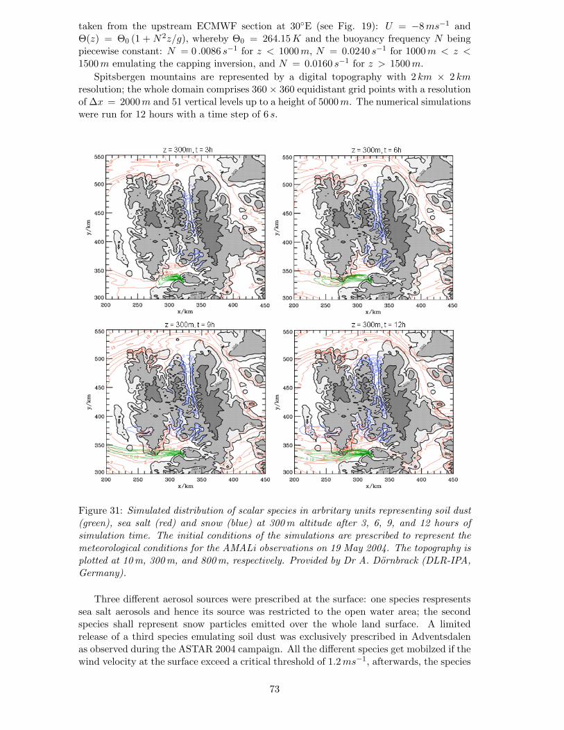
taken from the upstream ECMWF section at 30◦E (see Fig. 19): U = −8 ms−1 andΘ(z) = Θ0 (1 + N2z/g), whereby Θ0 = 264.15 K and the buoyancy frequency N beingpiecewise constant: N = 0 .0086 s−1 for z < 1000 m, N = 0.0240 s−1 for 1000m < z <1500 m emulating the capping inversion, and N = 0.0160 s−1 for z > 1500 m.

Spitsbergen mountains are represented by a digital topography with 2 km × 2 kmresolution; the whole domain comprises 360 × 360 equidistant grid points with a resolutionof Δx = 2000 m and 51 vertical levels up to a height of 5000m. The numerical simulationswere run for 12 hours with a time step of 6 s.

Figure 31: Simulated distribution of scalar species in arbritary units representing soil dust(green), sea salt (red) and snow (blue) at 300m altitude after 3, 6, 9, and 12 hours ofsimulation time. The initial conditions of the simulations are prescribed to represent themeteorological conditions for the AMALi observations on 19 May 2004. The topography isplotted at 10m, 300m, and 800m, respectively. Provided by Dr A. Dornbrack (DLR-IPA,Germany).

Three different aerosol sources were prescribed at the surface: one species respresentssea salt aerosols and hence its source was restricted to the open water area; the secondspecies shall represent snow particles emitted over the whole land surface. A limitedrelease of a third species emulating soil dust was exclusively prescribed in Adventsdalenas observed during the ASTAR 2004 campaign. All the different species get mobilzed if thewind velocity at the surface exceed a critical threshold of 1.2 ms−1, afterwards, the species

73

get vertically mixed by the turbulent flow past the Svalbards mountains. The mobilizationphase of the species was modelled according to the formulas presented by Nickovic andDobricic [137]. In this preliminary simulations, the same value of the effective amount ofaerosol mobilized at ground was applied for all species.

Figure 31 despicts the temporal evolution of the aerosol distribution every 3 hours byhorizontal cross-sections at 300 m altitude. Due to the strong corner-wind at the northerntip of Svalbard and the associated enhanced vertical mixing the simulated sea salt aerosolconcentration increases with time. This produces a pronounced meridional concentrationgradient toward the wake region further south which is less loaded with aerosol. Thus, thesimulation results are in qualitative agreement with the lidar observations: the increasedaerosol concentration found in the profiles of the yellow category presented in figure 30was most likely caused by sea salt aerosols. Also the sharp concentration gradient foundin the lidar observations is well reproduced by the model simulations. The lowest aerosolcontent is simulated west and north-west offshore Prins Karls Forland and can be linkedto the low backscatter ratios obtained for the pink category profiles in figure 30.

The enhanced aerosol concentration around the mouth of Isefjord was simulated asconsisting of a mixture of soil dust and sea salt aerosol. Generally, this is in accord withthe observed increase of lidar backscatter in the lowest 300m. However, whether thedust really contributed to the enhanced backscatter must be studied in the future. In thenumerical simulations a continous dust source was prescribed; however, the dust eventterminated about 24 hours before the airborne observation. Thus, a realistic simulation ofthe dust particle emission and transport including sedimentation for a longer period mustbe done in the future.

It is interesting to note that the numerical model calculated a plume consisting of snowand sea salt without dust in the area south-west offshore Prins Karls Forland (c.fig. 31,simulation time t = 12 h). At higher vertical levels, the enhanced aerosol concentration isdominated by snow with maximum values between 1000m and 1500m altitude. Here, onecan only speculate if the observed backscatter maximum at about 10:45 UT in figure 22was generated by drifting ice particles which could not sink due to the large positivevertical velocity in this region (c.fig. 19). Again, a more realistic simulation of the particleproperties of snow will give an answer. At the end, the lidar observations will be used toimprove the aerosol parametrizations in EULAG in future studies.

5.10 Observations of mixed-phase clouds with alternated AMALi andin-situ instrumentation

The investigations of climate change due to clouds with respect to changes of cloud radia-tive properties (altitude, area coverage and cloud properties), changes due to indirect effectof aerosols on cloud formation, and changes due to cloud modification on ice pack, arelately recognized important, especially in climatologically pivotal areas such as the Arctic(c.cpt. 1). The information on the properties of arctic clouds, though few campaigns werededicated to perform clouds measurements in Arctic (c.cpt. 2), is relatively scant, whichmakes the modelling of the aerosol-cloud-climate interactions especially challenging.

The measurements carried out during ASTAR 2004 campaign in the vicinity of Sval-bard Archipelago can well contribute to such collaborative studies since Svalbard is awell-fitting spot to assess the scientific issues mentioned above. The montainous orog-raphy of the archipelago allows for measurements over various distinct terrains. Thesuitable geographical position with its permanently maintained research stations, as forexample Koldewey Station, Rabben Station, Zeppelin Mountain Station, Hornsund Sta-tion (c.cpt. 2.1.2), an access to logistic for research aircrafts at the airports in Longyearbyenand Ny-Alesund (c.cpt. 2.1.1), together with a space observations from polar orbital satel-lites, for example future CALIPSO or CLOUDSAT makes Svalbard even more interesting

74

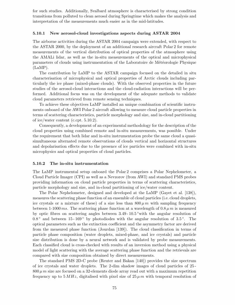
for such studies. Additionally, Svalbard atmosphere is characterised by strong conditiontransitions from polluted to clean aerosol during Springtime which makes the analysis andinterpretation of the measurements much easier as in the mid-latitudes.

5.10.1 New aerosol-cloud investigations aspects during ASTAR 2004

The airborne activities during the ASTAR 2004 campaign were extended, with respect tothe ASTAR 2000, by the deployment of an additional research aircraft Polar 2 for remotemeasurements of the vertical distribution of optical properties of the atmosphere usingthe AMALi lidar, as well as the in-situ measurements of the optical and microphysicalparameters of clouds using instrumentation of the Laboratoire de Meteorologie Physique(LaMP).

The contribution by LaMP to the ASTAR campaign focused on the detailed in situcharacterisation of microphysical and optical properties of Arctic clouds including par-ticularly the ice phase (mixed-phase clouds). With the observed properties in the futurestudies of the aerosol-cloud interactions and the cloud-radiation interactions will be per-formed. Additional focus was on the development of the adequate methods to validatecloud parameters retrieved from remote sensing techniques.

To achieve these objectives LaMP installed an unique combination of scientific instru-ments onboard of the AWI Polar 2 aircraft allowing to measure cloud particle properties interms of scattering characteristics, particle morphology and size, and in-cloud partitioningof ice/water content (c.cpt. 5.10.2).

Consequently, a development of an experimental methodology for the description of thecloud properties using combined remote and in-situ measurements, was possible. Underthe requirement that both lidar and in-situ instrumentation probe the same cloud a quasi-simultaneous alternated remote observations of clouds vertical and horizontal structuresand depolarisation effects due to the presence of ice particles were combined with in-situmicrophysics and optical properties of cloud particles.

5.10.2 The in-situ instrumentation

The LaMP instrumental setup onboard the Polar 2 comprises a Polar Nephelometer, aCloud Particle Imager (CPI) as well as a Nevzorov (from AWI) and standard PMS probesproviding information on cloud particle properties in terms of scattering characteristics,particle morphology and size, and in-cloud partitioning of ice/water content.

The Polar Nephelometer, designed and developed at the LaMP (Gayet et al. [138]),measures the scattering phase function of an ensemble of cloud particles (i.e. cloud droplets,ice crystals or a mixture of these) of a size less than 800 μ m with sampling frequencybetween 1-1000 ms. The scattering phase function at a wavelength of 0.8μ m is measuredby optic fibres on scattering angles between 3.49 - 10.5 ◦with the angular resolution of0.8 ◦ and between 15 - 169 ◦ by photodiodes with the angular resolution of 3.5 ◦. Theoptical parameters such as the extinction coefficient and the asymmetry factor are derivedfrom the measured phase function (Jourdan [139]). The cloud classification in terms ofparticle phase composition (water droplets, mixed-phase, and ice crystals) and particlesize distribution is done by a neural network and is validated by probe measurements.Each classified cloud is cross-checked with results of an inversion method using a physicalmodel of light scattering with the average scattering phase function and the retrievals arecompared with size composition obtained by direct measurements.

The standard PMS 2D-C probe (Reuter and Bakan [140]) provides the size spectrumof ice crystals and water droplets. The 2-dim shadow images of cloud particles of 25 -800 μ m size are focused on a 32-elements diode array read out with a maximum repetitionfrequency up to 5MHz, digitalised with pixel size of 25μ m with temporal resolution of

75

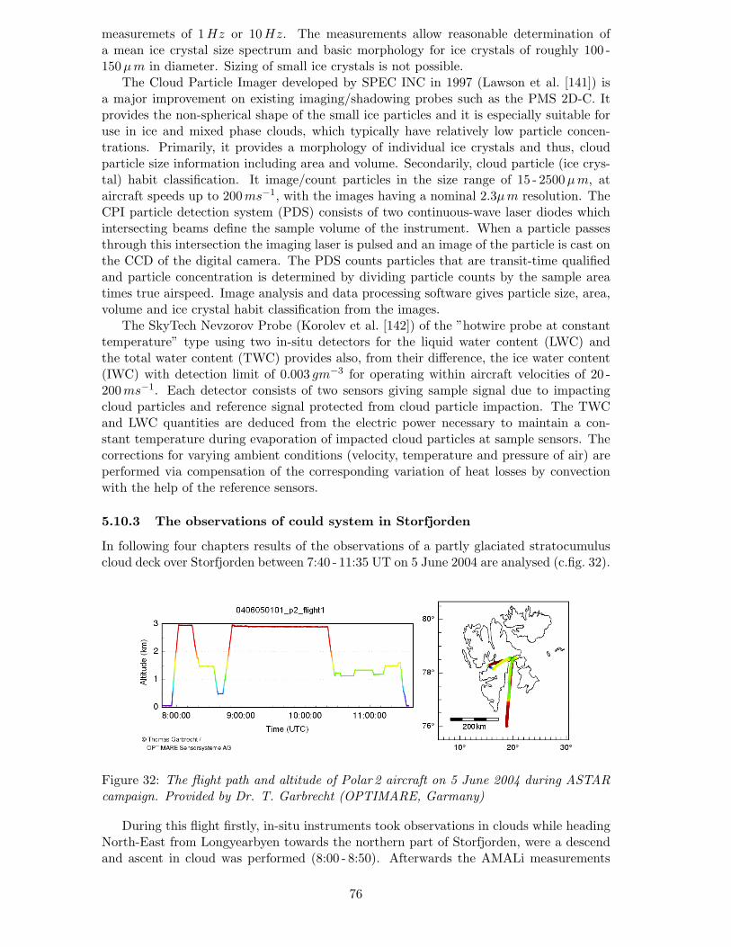
measuremets of 1 Hz or 10 Hz. The measurements allow reasonable determination ofa mean ice crystal size spectrum and basic morphology for ice crystals of roughly 100 -150 μ m in diameter. Sizing of small ice crystals is not possible.

The Cloud Particle Imager developed by SPEC INC in 1997 (Lawson et al. [141]) isa major improvement on existing imaging/shadowing probes such as the PMS 2D-C. Itprovides the non-spherical shape of the small ice particles and it is especially suitable foruse in ice and mixed phase clouds, which typically have relatively low particle concen-trations. Primarily, it provides a morphology of individual ice crystals and thus, cloudparticle size information including area and volume. Secondarily, cloud particle (ice crys-tal) habit classification. It image/count particles in the size range of 15 - 2500μ m, ataircraft speeds up to 200 ms−1, with the images having a nominal 2.3μ m resolution. TheCPI particle detection system (PDS) consists of two continuous-wave laser diodes whichintersecting beams define the sample volume of the instrument. When a particle passesthrough this intersection the imaging laser is pulsed and an image of the particle is cast onthe CCD of the digital camera. The PDS counts particles that are transit-time qualifiedand particle concentration is determined by dividing particle counts by the sample areatimes true airspeed. Image analysis and data processing software gives particle size, area,volume and ice crystal habit classification from the images.

The SkyTech Nevzorov Probe (Korolev et al. [142]) of the ”hotwire probe at constanttemperature” type using two in-situ detectors for the liquid water content (LWC) andthe total water content (TWC) provides also, from their difference, the ice water content(IWC) with detection limit of 0.003 gm−3 for operating within aircraft velocities of 20 -200 ms−1. Each detector consists of two sensors giving sample signal due to impactingcloud particles and reference signal protected from cloud particle impaction. The TWCand LWC quantities are deduced from the electric power necessary to maintain a con-stant temperature during evaporation of impacted cloud particles at sample sensors. Thecorrections for varying ambient conditions (velocity, temperature and pressure of air) areperformed via compensation of the corresponding variation of heat losses by convectionwith the help of the reference sensors.

5.10.3 The observations of could system in Storfjorden

In following four chapters results of the observations of a partly glaciated stratocumuluscloud deck over Storfjorden between 7:40 - 11:35 UT on 5 June 2004 are analysed (c.fig. 32).

Figure 32: The flight path and altitude of Polar 2 aircraft on 5 June 2004 during ASTARcampaign. Provided by Dr. T. Garbrecht (OPTIMARE, Garmany)

During this flight firstly, in-situ instruments took observations in clouds while headingNorth-East from Longyearbyen towards the northern part of Storfjorden, were a descendand ascent in cloud was performed (8:00 - 8:50). Afterwards the AMALi measurements

76

were taken at a flight altitude of 3 km while heading strait into southern part of Storfjorden(9:00 - 10:20). During these observations the cloud structures were observed over an icecovered northern part of the fiord and the background aerosol profiles were taken in acloud-free area over open water just outside the fiord. Finally, after a descent into themarine stratocumulus cloud layer, the heading back along the same flight path (10:30 -11:30) but at altitudes between 1.1 - 1.5 km towards the northern end of Storfjorden whilethe in-situ observations were performed.

The water stratocumulus cloud top was about -12◦C, not unusual in the Arctic (c.cpt. 5.8).Over the Beaufort Sea at altitudes below 2 km and temperatures down to −9◦C cloudsgenerally contain purely liquid particles with the lowest concentration of cloud formingparticles due to precipitation and nucleation scavening in the boundary layer (Pinto etal. [133]).

At upper levels ice particles were evidenced to precipitate down to the stratocumuluslayer leading to a possible feeder-seeder phenomenon within the water cloud. Therefore,three kinds of clouds with different microphysical and optical properties, i.e. precipitatingice crystals, mixed-phase cloud and water layer cloud with large drops, were evidencedfrom both measurements.

5.10.4 The remote sampling with AMALi

The AMALi contribution to this experiment was useful in two ways. Firstly, the avail-ability of the real-time display of the quick-look evaluation of the measured atmosphereallowed for an immediate in-flight interpretation of lidar signals at 532nm and 1064nmand a depolarisation ratio at 532nm. Hence, recognition and guidance of in-situ observa-tions into the areas of particular research interest was possible (c.cpt. 3.2.4).

Secondly, after the flight, the calculation of calibrated backscatter profiles at se-lected times along the flight path and in the regions of low density clouds was possible(c.cpt. 5.10.6) using the iterative airborne lidar inversion scheme considering Klett-Fernaldmethodology (c.cpt. 4.6 and 5.5).

Figures 33 and 34 represent the AMALi signals and the depolarisation ratio at 532nmrecorded during the flight sequence performed at 3 km (maximum Polar 2 aicraft ceiling).

During the first part of the measurement, between 8:57 - 9:15 precipitating ice particlesare clearly evidenced. At some parts of the cloud system in this time interval the icecrystals seem to reach the water cloud below (9:00 - 9:05 and 9:10 - 9:15).

At the very first part of the measurements between 8:58 - 9:02 the double structure ina lower cloud deck with an ice cloud at an altitude of about 1.5 km topped by a watercloud at about 1.75 km was observed. Otherwise, the lower deck cloud contained highlyconcentrated spherical particles of low depolarisation ratio of 1.4 - 5 %.

In the upper cloud layer the depolarisation ratio increases from 25 - 30 % to 40 - 50 %which clearly reveal the occurrence of irregularly shaped ice crystals. We may expect theseice crystals precipitation down to the water cloud layer at 1.4 km altitude. Then, due toFindeisen-Bergeron process the ice crystals may grow to the detriment of supercooledwater droplets as far as most of them may be consumed. Nevertheless, the observationsdo not confirm this hypothesis since the precipitating down to the ground stratocumulusfeature (9:16 - 9:21) rather highlights depolarisation ratio as low as 1.4 % to 5 % typical foronly spherical particles and hence for freezing drizzle.

The second part of the measurements between 9:22 - 9:35 UT was taken in a cloud-freeatmosphere above a dense liquid cloud of about 150 - 200m depth extending horizontallyover about 65 km at an altitude of about 1.5 km. The laser beam in both lower deck waterclouds was rapidly attenuated due to very high concentration of the scattering centresresulting in the multiple scattering. Hence, the lidar signals and depolarisation ratio belowthese clouds and the sea level cannot be exploited in the further analysis (Weinman [143]).

77

The signals above these clouds reveal, due to a weaker beam attenuation, distinct cloudstructures containing either large non-spherical particles or spherical particles with a lowerconcentration.

The final part of the measurement between 9:36 - 9:42 UT was taken in a cloud-freebackground atmosphere. The noisy character of depolarisation ratio profiles observedin the clear atmosphere areas is due to lower target concentrations than in aerosol-richatmosphere or in clouds resulting in a weaker backscatter signal at perpendicular 532nmwavelength.

Figure 33: The vertical cross-section of the attenuated AMALi lidar signal at 532nm formeasurements of the mixed-phase clouds between 8:57-9:42 on 5 June 2004 during ASTAR

Generally, in case of atmospheric regions with very low concentrations of scatteing cen-tres backscatter detection at any lidar wavelength is limited. For example, the scatteringdetection at 1064 nm in very clear atmosphere is usually limited due to the lack of largescattering centres. However, as soon as large particles (dust, large water droppletsor icecrystals) appear the detection of these can be done (c.fig. 10).

Similarly, the perpendicular 532nm detection with the backscatter signals intensities102 - 103 times weaker as for the parallel 532 nm detection, the low densities of the scat-tering centres in clear arctic atmosphere limit its detection ability, so that the existence ofnoisy returns in this areas is typical. Hence, the representative mean value of depolarisa-tion ratio of 5.4 % in the clear parts of atmosphere above the water cloud and in cloud-freeatmosphere between 9:25 - 9:42 UT was found.

The calculations using the iterative airborne backward Klett inversion algorithm (c.cpt. 4.6)allow for the retrieval of the calibrated particle backscatter coefficient along the flight pathin areas where the optical depth of the clouds is low enough, i.e. lower than the thresholdparticle optical depth of 0.065 in a 100m thick cloud layer. However, for these calculationsthe lidar ratio has to be assumed.

Usually, for most retrievals of the AMALi observations under clean clear-sky conditions

78

during ASTAR, the constant lidar ratio of 20 - 25 srad can be assumed (c.cpt. 5.5, errordiscussion). Theoretically, for the calculations in water clouds the lidar ratio can beobtained from the Mie-theory if, usually difficult, guess of the size of the particles is made.For the ice particles such calculations make hardly sense due to their non-spherical shape,however, if the clouds contain mainly ice crystals an assumption of a lidar ratio between12 - 15 srad can be made (Ansmann et al. [96]).

Unlike for the usual approach where the lidar ratio is estimated (Carnuth and Re-iter [144], Young [145]), this approach allows an application of the iterative Klett algo-rithm to clouds of low optical densities penetrable with the laser beam without causing themultiple scattering the accurate calculations are done with lidar ratio depending on typeof cloud (water/ice) obtained from in-situ observations. The backscatter profiles obtainedwith such lidar ratios are presented and discussed in chapter 5.10.6).

Figure 34: The vertical cross-section of the depolarisation ratio at 532nm for measure-ments of the mixed-phase clouds between 8:57-9:42 on 5 June 2004 during ASTAR

5.10.5 The in-situ sampling with cloud microphysics instrumentation

The in-situ probes provided cloud characteristics in terms of particle size distribution,concentration, ice/liquid water content, morphology, scattering phase function, refractiveindex and asymmetry factor.

The particle size distributions for water and ice clouds obtained form PMS 2D-Cprobe and the Polar Nephelometer (after inversion) is depicted on figure 35. Generally,in both types of clouds rather small size cloud droplets with size less than 200μ m andwith no super-large drops were observed. For both types of clouds the concentrationof the small size particles with effective diameter around 25 μ m is similar but for the icecloud a significant fraction of larger particles with effective diameter of around 200μ m wasmeasured. The particle concentrations of 8 ·103l−1 with particle extinction of 10 ·10−3m−1

in water cloud and much lower concentrations of 11 l−1 and particle extinction of 0.4 ·

79

10−3m−1 in ice cloud were retrieved. In case of a water cloud relatively high concentrationof small size droplets are present with absence of large particles. On the contrary, for theice cloud, the presence of sufficiently large particles causes its ’precipitating’ character.

The Nevzorov Probe measured 80 mg m−3 liquid water content in the water cloud and4.3 mg m−3 ice water content in ice cloud, respectively.

Figure 35: The particle size distributions for water cloud (left) and ice cloud (right) ob-tained form PMS 2D-C probe (red) and retrieved from the Polar Nephelometer (green)measurements taken on 5 June 2004 during the ASTAR campaign. Provided by Dr. J.-F.Gayet (LaMP, France)

Figure 36: The scattering phase function for water cloud (left) and ice cloud (right) ob-tained from Polar Nephelometer for measurements taken on 5 June 2004 during the AS-TAR campaign. Provided by Dr. J.-F. Gayet (LaMP, France)

The measurements of the scattering phase function for water and precipitating icecrystals obtained with the Polar Nephelometer are shown on figure 36. Characteristicdeep minimum due to the spherical particles for the the water cloud is evidenced. Foreach recognized cloud particle phase composition (water droplets and ice crystals) theoptical parameters such as the extinction coefficient, the asymmetry factor and the lidar

80

ratio were derived from the measured scattering phase function (Jourdan et al. [139]).The lidar ratio of 14.5 srad and, as expected for the ice clouds, a bit lower of 13.8 srad for532 nm were obtained.

As these results (c.fig. 36) represent mean values obtained during sequences of 2 min forthe water cloud and 7min for the ice cloud, respectively, they are considered statisticallyreliable due to a very large sampled volume. The natural variability, generally high inany cloud types, is not considered in these results. The statistical errors on microphysicalmeasurements are discussed in details in Gayet et al. [54].

5.10.6 The comparison of the remote and in-situ particle backscatter andextinction retrievals

The figure 37 shows particle backscatter profiles obtained with 2min temporal resolutioncorresponding to about 8 km range calculated using the iterative aproach with lidar ratioscorresponding to ’ice cloud’ and ’water cloud’ retrieved from the in-situ measurements and’clear air’ lidar ratios assumed to be 25 srad.

Figure 37: Particle backscatter coefficient retrieved for the preselected regions of the mixed-phase cloud; ice cloud (1-3), drizzle(4), and coloud-free atmosphere (5,6) from the AMALimeasurements at 532 nm during the flight on 5 June 2004 at ASTAR campaign. The CPIimages of the ice crystals and water dropplets attributed to each type of cloud were providedby Dr. J.-F. Gayet (LaMP, France)

The profiles no. 1 - 3 were obtained at 9:00, 9:08 and 9:13 in the area of the precipitatingice crystals. The profile no. 4 was obtained at 9:19 in the drizzle and could be retrieveddown to the sea level. The profile no. 5 at 9:27 was obtained in a clear atmosphere abovethe liquid cloud and, finally, the profile no. 6 at 9:37 in the cloud-free atmopshere wascalculated as a reference profile.

The last two profiles were compared for a consistency with the three categories of thedifferent types of the backscatter ratio profiles discussed in chapter 5.9.1. Their shapefits the ’clear air’ of the pink category well, though the values of the backscatter ratios

81

retrieved on 5 June 2004 are slightly higher, with a background backscatter ratio around1.8 and a maximum of 3 near the sea level.

The lidar particle extinction coefficient of a 0.07 · 10−3m−1 in the ice cloud area wasretrieved for backscatter value of 0.5 ·10−5m−1srad−1 estimated from particle backscattercoefficient profiles no. 1 - 3 with corresponding ’ice cloud’ lidar ratio of 13.8 srad.

The lidar particle extinction coefficient of 0.61 · 10−3m−1 in the drizzle area was re-trieved for maximum of the particle backscatter value of 4.2 · 10−5m−1srad−1 estimatedfrom backscatter profile no. 4 with corresponding ’water cloud’ lidar ratio of 14.5 srad.

The in-situ particle extinction coefficient of a 0.05 - 0.4·10−3m−1 in the ice cloud and1 - 10·10−3m−1 in the drizzle was obtained.

The comparison of particle extinction from remote and direct observations shows sim-ilar values in ice clouds and significant differences in drizzle case which can be explainedby the time shift between both measurements and by a possible increase of the drizzle for-mation. The drizzle intensification seems also be reasonable from the analyses of the lidarsignals alone. The calculations of particle backscatter profiles in ’cloudy’ area is possibleonly within the range of mentioned threshold values of the particle extinction of less than0.65 · 10−3m−1. Hence, the lidar measurements in the intense drizzle sampled by in-situinstrumentation for which the particle extinction coefficient of more than 1 · 10−3m−1

would not be possible, due to the multiple scattering on these drizzle particles.

Comments on the alternative measurement approachThe airborne remote and in-situ cloud studies comprising the instrumentation on-

boardof the two aircrafts have been widely used in the ’cloud’-community (Gayet etal. [146]). However, to my knowledge, these are the first observations proving the feasabil-ity of the alternated measurement approach possible if only one aircraft is available.

The combined analysis of remote and in-situ measurements allowed for characterisationof mixed-phase Arctic clouds and for attributing different particle shapes (spherical andnon-spherical) to distinct zones of the cloud system. In case of the observations of afeeder-seeder phenomenon three kinds of clouds with different microphysical and opticalproperties; the precipitating ice crystals, the mixed-phase cloud and the water layer cloudwith large drops were found. The identification of vertical and horizontal structures ofmixed-phase clouds, the identification of typical signatures of drizzle and ice clouds andthe derivation of the typical ice-cloud and liquid-cloud lidar ratios was possible.

The cross-check of the retrieved lidar backscatter and extinction with the in-situ ob-servations proves the feasibility of the alternated probing approach. Though, to improvethe methodology more observations coordinated in space and time are necessary.

The lidar measurements of cloud areas and their direct surrounding give an idea onthe atmospheric ’dynamics’. It allow to constrain the open questions on whether thesurrounding area is entirely clear or contaminated with some cloud particles, as for examplein the case of the water drops above boundary cloud deck found between 9:19 and 9:23 inthe depolarisation ratios in figure 34. Or whether there is some aerosol associated withthe sampled clouds, as for example in the case of the strong aerosol gradients found onthe boarder of Foehn-like boundary clouds in figure 22.

Finally, this approach will be continued for the validation of the satellite cloud obser-vations during future ASTAR campaigns, and the results obtained from such alternatedmeasurements should contribute to the modelling of aerosol-cloud-climate interactions.

82

6 Conclusions and Outlook

The AMALi lidar system constructed and built at the beginning of this project almostthree years ago was implemented in many ways for the lower troposphere investigations.

Before the Arctic campaigns took place the system was validated and tested duringJanuary-April 2004 while performing ground based investigations of diurnal cycle fromthe AWI Lidar Laboratory in Potsdam. Additionally, the robust construction and thetrouble-free operation of the AMALi lidar allowed for the airborne investigation of thesea-land gradients over the north-western coastline offshore Bremerhaven during the lidartest-campaigns in April 2004 and March 2005.

During the ASTAR 2004 campaign extensive airborne observations of atmosphericevents were performed, just to mention few,

- airborne observations of an extend of the local dust plume over Adventdalen,- investigations of the aerosol gradients between different air masses in North and

South offshore the west coast of Spitzbergen,- investigations of the wave-driven aerosol structures in the same area,- marine boundary layer observations over the Isfjord,- combined airborne AMALi, ground based KARL, and ground based remote and

in-situ instrumentation at the research stations in vicinity of Ny-Alesund,- investigations of the difference in boundary layer aerosol content over- ice covered sea and the open water sea over the Storfjord by combined remote and

in-situ Polar 2 and Polar 4 observations,- alternated AMALi and in-situ measurements of cloud structures and mixed-phase

cloud optical and microphysical characteristics,- AMALi and in-situ investigations of characteristic falling streaks of a diamond dust,- investigations of air masses offshore the Sorkappland combined with the in-situ ob-

servations at the Polish Station in Hornsund.Additionally, the ground based AMALi and KARL intercomparison experiment and

the ground based AMALi horizontal measurements over Kongsfjord both taken from theAWI’s Koldewey Research Station in Ny-Alesund were performed.

During the SVALEX 2005 campaign the Arctic haze observations aimed to provide acharacteristic, horizontal extents and an assessment of the temporal evolution of such eventon a small-scale. These were followed by the observations of the polluted air mass spatialand temporal variability, including orographical effects, via parallel and perpendicularmeasurements with respect to the uniform movement of the polluted air mass.

In the frame of this PhD thesis it is not possible to discuss all of these experiments,hence, the most important results had to be selected to be presented. In the next twochapters comments on each of the issues under concern, as well as an outlook for the futurework is summarised.

6.1 Comments on the aerosol and clouds studies described in the frameof this work

Comments on the advantages of the precise knowledge of the lidar constantFor most of the backscatter lidar systems I was acquainted with, the lidar instrumental

constant was not known precisely or even not at all, mainly due to the fact that mostof these systems used the Klett’s evaluation approach for which the lidar instrumentalconstant is redundant. In this work a way to determine the airborne and ground basedlidar instrumental constants precisely was developed and opened a few new aspects forthe optical and microphysical parameter retrieval from the backscatter lidar data.

83

It allowed for the improvement of the Klett’s backward approach for the retrieval ofthe calibrated backscatter ratio profiles from the airborne backscatter lidar data, even ifthe calibration value is not avaliable or cannot be accurately assumed.

It allowed also for the precise estimation of the initial backscatter calibration value forthe application of the Klett’s forward approach for the backscatter coefficient retrieval.

Furthermore, it allowed for the successful implementation of the two-stream method-ology for the precise calculations of the backscatter coefficient, without the knowledge ofthe lidar ratio and the calibration value.

Additionally, at least theoretically, it allows for the direct calculation of the aerosolmicrophysical properties from the range corrected lidar signals, i.e. independently fromthe extinction and backscatter retrievals.

Comments on the two-stream methodologyThe two-stream method is an interesting tool for data evaluation from combined lidar

measurements. It proved feasible for the AMALi airborne and KARL ground based datavalidation and evaluation at a polar site.

In unstable meteorological conditions, it is important that both instruments probethe very same air. However, a simple comparison (divison) of both range corrected lidarsignals allows for the assesesment of the appriopriate range for the two-stream application.

The two-stream extinction coefficients were retrieved more precisely than with theAnsmann evaluation approach of the Raman lidar. In the two-stream extinction coefficientprofiles, unlike for the Raman retrieval, the main limitation of the obtained profile rangeis due to the flight altitude of the avaliable airborne/spaceborne craft.

In case that any of the two instruments observes a layer with low or known particlecontamination, the lidar constant of this instrument can be precisely determined. Hence,the two-stream backscatter coefficient can be calculated. In the two-stream method, unlikefor the Klett inversion, an error of the backscatter calibration causes only bias on theretrieved backscatter profile, i.e. it only shifts the whole profile by a constant value.

Generally, the errors of the two-stream solutions are mainly due to the assumptionthat both lidars are sampling into exactly the same atmosphere. Hence, in reality theretrieval is possible only if the stability of the measured atmospheric layers lasts a longertime than the time resolution of the airborne lidar sampling.

The application of the two-stream approach for the extinction and the backscatterretrievals from combined ground based and satellite lidar measurements seem feasible aswell. Though, the fact that one of the involved instruments in the two-stream methodmust be air/spaceborne makes this approach quite expensive to be used on everyday basis.However, during future campaigns an ample use of this technique shall be made.

Therefore, especially interesting, is a planned contribution towards validation and anal-ysis of the lidar data obtained from the CALIPSO satellite, which will frequently overflythe polar regions, using the two-stream technique applied to the CALIPSO lidar and theKARL lidar and/or the zenith-aiming AMALi lidar.

Comments on the clean ASTAR contra polluted SVALEX aersosol characteristicsThe two-stream method was successfully applied to both clean and polluted (Arctic

haze) Arctic air measurements during the clear-sky conditions in the Foehn-gap formedNorth-West off Svalbard Archipelago. The measurements taken in such interestingly con-ditions allowed for the comparision of both observations, though they were taken duringtwo campaigns; the ASTAR on 19 May 2004 and the SVALEX on 14 April 2005.

The optical properties of investigated atmosphere on each of these days obtained fromthe two-stream approach were compared between each other and interpreted in terms oftheir optical properties (extinction, backscatter, depolarisation, optical depth), microphys-ical parameters (refractive index, size distribution and particle number concentration) and

84

meteorological properties (humidity, temperature, origin) providing ’clean’ contra ’haze’characteristics.

During the ’clean’ day the background values characteristic for the clean Arctic air wereretrieved with the particle extinction coefficient varying around 1.5·10−5m−1, the particlebackscatter coefficient between 0.3 - 0.7·10−6m−1srad−1 and the lidar ratio of 20 srad witha corresponding complex refractive index m = 1.4 + 1·10−4 i typical for water particles anda bimodal size distribution dominated with only a few large particles of the effective radiusvarying between 0.6 - 1.2 μm, very narrow σ of 1.26, and very low particle concentrationsbetween 0.5 - 3 cm−3. The long-range air mass transport together with the retrieved valuesof the microphysical and the optical properties suggest that no anthropogenic pollutantswere mixed into this air.

A year later, strongly enhanced particle extinction coefficients between 3 - 8·10−5m−1,the particle backscatter coefficients between 0.9 - 2.2·10−6m−1srad−1 and the lidar ra-tios of about 35 srad were obtained. The corresponding complex refractive index m =1.68 + 3 ·10−3 i, typical for anthropogenic aerosol, with noticeably increased value of Re mindicated possible soot contaminations, common for Arctic haze. The size distribution wascharacterised by a monomodal log-normal distribution with the effective radius of 0.2 μmwith σ of 1.7 and high particle concentrations varying between 50 - 150 cm−3. The long-range air mass transport indicated the area of Lena Delta and Yenissey Delta as a sourceof pollution, while the high extinction of this air, its uniform character of the well mixedair within the lower troposphere excludes a local source for the observed aerosol load.

Comments on the evidence of the humid layers in Ny-AlesundMost of the profiles retrieved with the two-stream inversion during the ASTAR and

the SVALEX campaigns showed an evidence of well pronounced layers characterised bya strongly enhanced particle extinction coefficient and lidar ratio, undiscernible in thebackscatter coefficient profiles.

Such a characteristic of the optical parameters usually suggests possible contaminationby small amounts of soot particles, which have an effect in enhancement of the extinctioncoefficient due to its strong absorption of the VIS-radiation. However, an existence ofrather a large number of small, supercooled water droplets in the mentioned layer wasalso credible.

As possible causes for the existence of these layers the following were considered: thecontaminations with soot pollutants of local or ’advective’ origin; the occurence of theprecondensation conditions as a subvisible clouds; the increase of the relative humidity withthe fall of the temperature characteristic for the Foehn-pause formed by the orographicwave retreat; and finally, the cumulation of the particles under a stable, thin inversionlayer caping the mountain gap flow layer on the downstream flow into the Kongsfjordvalley.

The microphysical parameters justified a contamination by small amounts of soot par-ticles only in one of these layers. The long-range air mas transport showed both the massorigin in the high Arctic or at the lower rather polluted latitudes. The layers occuredduring both, the Foehn-like events and the ’normal’ clear-sky conditions.

However, all found layers were strongly dependent on the existence of the temperatureinversion, evidenced from the radio sounding. Also the microphysical parameters inversionresults showed large number (50 - 300 pcm−3) of small-sized (around 200nm) particles forall layers.

Hence, the local origin of such layers containing a large number of small, supercooledwater droplets cumulated just below the inversion layers caused by a meteorological distur-bance due to the flow of the air mass over the rough mountains surrounding Kongsfjordenis most credible.

On a methodology point of view it is interesting to note that the observations of such

85

layers visible only in the extinction and the lidar ratio profiles underline the necessity ofa determination of the backscatter and the extinction coefficients independently of eachother from lidar measurements. Hence it underlines the necessity of the Karl’s Ramanapproach, the airborne AMALi and KARL two-stream approach and the horizontally-aiming AMALi slope approach for the proper data evaluation.

Comments on the AMALi iterative algorithmThe advantage using an iterative approach proposed in this thesis providing a cali-

brated quantitative information on the particle backscatter coefficient instead of the qual-itative range and background signals provided typically by airborne lidars is clear.

In contrary to most of the airborne evaluation approaches requiring the difficult as-sessment of the calibration value along the flight in the aerosol rich lower troposphere oradditional instrumentation for its measurement, here the method of its precise calculationfrom the lidar signal alone was discussed and succesfully applied to the AMALi data.

The knowledge of the calibration value at any time during the flight allowed for pro-viding the backscatter ratio profiles under the clear-sky conditions, obtained with theassumption of the constant lidar ratios of 20 - 25 srad for clear arctic air and 30 - 35 sradfor polluted arctic air. This assumption was found to be not too critical to retrieve ac-curate backscatter ratio due to a short range of AMALi measurements (2.7 km) under,usually, a very stable Arctic atmosphere and a quasi-uniform air mass transport. For theflights where the air mass transport had non-uniform character and the contaminationwith pollutants can be expected at a particular altitudes the height dependent lidar ratiowas assumed. However, the sensitivity studies for both types of the retrievals showed nosignificant hindering, i.e. errors less than 2 · 10−7 m−1srad−1 were obtained.

Additionally, the iterative approach was used also to determine the particle backscatterfor the observations in the mixed-phase clouds, as long as their low optical densitiesallowed penetration with the laser beam without causing the multiple scattering. For thecalculations in clouds a guess of the lidar ratio is very difficult due to the fact that thepartial derivative of the backscatter coefficient over lidar ratio increases with the increaseof the backscatter coefficient, i.e. the errors are much larger in clouds. Hence, for thesecalculations a lidar ratio dependent on type of cloud has to be obtained from the in-situcloud observations.

Comments on the alternated remote and in-situ cloud measurement methodologyTo my knowledge, in this thesis the first observations comprising the airborne remote

and in-situ cloud studies proving the feasibility of the alternated approach utilising onlyone aircraft was presented.

The alternated lidar and in-situ measurements allowed for characterisation of mixed-phase Arctic clouds and for attributing different particle shapes (spherical and non-spherical) to distinct zones of the investigated cloud system.

In the case study of the feeder-seeder phenomenon described in this thesis three kindsof clouds with different microphysical and optical properties were found: the precipitatingice crystals, the mixed-phase cloud and the water cloud with large drops.

The identification of the vertical and horizontal structures of the mixed-phase clouds,the identification of the typical signatures of drizzle and ice clouds, and the derivationof the typical ’ice-cloud’ (13.8 srad) and the typical ’liquid-cloud’ (14.5 srad) lidar ratioswere possible.

Additionally, the lidar measurements of the cloud areas and the direct surroundingair gave an idea on the ’cloud-dynamics’ by assessing whether the surrounding is entierlyclear or contaminated with a particular type of aerosol, water or ice crystal particles.

The cross-check of the retrieved lidar backscatter and extinction with the in-situ obser-vations proved the feasability of the alternated probing approach. The comparison of the

86

particle extinction coefficient from remote and direct observations showed similar valuesin ice clouds (lidar: 0.07 · 10−3m−1, in situ: 0.05 - 0.4·10−3m−1) and significant differencesin drizzle case (lidar: 0.61 · 10−3m−1, in-situ: 1 - 10·10−3m−1). The latter difference canbe explained by the time shift of more than 30min between both measurements and bythe drizzle intensification.

In the future more observations coordinated in space and time are necessary for theimprovement of the methodology. The approach shall be continued for the validation of thesatellite cloud observations (CALYPSO, CLOUDSAT) during the ASTAR 2007 campaign.Finally, the results obtained from such alternated measurements should contribute to themodeling of aerosol-cloud-climate interactions.

Comments on the modelling activitiesThe knowledge about the origin, transport pathways and vertical structure of aerosol,

the physical and chemical properties of the aerosols and clouds including their interaction,as well as their impact on climate in the polar regions, can be greatly improved if acombined effort of complex ground based, airborne and spaceborne observations appliedtogether with regional scale climate modelling tools are implemented.

The collaborative studies on Arctic aerosol-cloud-climate interactions by combiningthe experimental data on aerosols/clouds properties together with models and the im-provement of the required parametrisation of radiation, aerosols and clouds processes areessential.

Each of the ASTAR campaigns provided detailed data sets of optical parameters ofArctic Haze and background conditions which can be used for parameterization of suchaerosols in the high resolution regional atmospheric climate model HIRHAM. Some of therequired by model sophisticated parameterizations of radiation, aerosol and cloud processesagainst the provided remote or in-situ observations, as for example the parametrisation ofclouds processes with temperature, are still under the development.

For such studies the data obtained during the combined Polar 2 for the AMALi aerosoland cloud measurements and the in-situ clouds measurements together with the Polar 4for the in-situ measurements of aerosols are highly valuable.

Presented in this thesis characteristics of the optical and microphysical parameters ofthe ’typical’ Arctic Haze (SVALEX 2005) and ’typical’ clean arctic conditions (ASTAR2004) retrived from combined AMALi and KARL measurements and from the microphys-ical parameters inversion code shall prove useful for the assessment of the impact of theArctic haze on climate using the HIRHAM model.

However, existing limitation for the implementation of the lidar information into theatmospheric regional models, including the comparatively small spatial and temopral scalecovered by the field campaigns, and the limited information on some parameters, whichcannot be directly provided by lidar measurements, as for example particle absorptioncoefficients, would have to be overcome.

Nevertheless, the new airborne investigations with the AMALi instrument open newdata sources for model investigations in two ways.

On one hand, as described in this thesis the obtained along the flight aerosol char-acteristics can be used for the local scale studies with the small-scale dispersion modelEULAG, and will find further application for the parametrisation of the different aerosoltypes in this model.

On the other hand, data sets representative for the regional scale will become avaliablethrough the application of the herein proposed methodologies applied to the airborneAMALi lidar and to the satellite borne lidar scheduled for lunch this winter (CALIPSO).

87

6.2 Recommendations for further research

Following is recommended to be performed in the future:- continuation of the two-stream approach for the airborne data evaluation during the

airborne campaigns for the AMALi and the KARL in their current configurations- validation of the satellite lidar by application of the two-stream approach to the

zenith-aiming KARL lidar and the CALIPSO satellite lidar at the satellite overpassesover the Koldewey Station

- validation of the satellite lidar by application of the two-stream approach to thezenith-aiming AMALi lidar measurements onboard Polar 2 flying partly along the flighttrack of the CALIPSO satellite lidar

- improvement of existing experimental procedure for aerosol-cloud-interaction inves-tigation using the AMALi and the LaMP in-situ instrumentation, also for the validationof the CLOUDSAT data and aerosol-cloud-interaction modelling

- direct implementation of the KARL’s lidar signals into microphysical parametersinversion code and feasibility study of this method

- investigation of the potential for implementation of the lidar-obtained vertical andhorizontal information on optical and microphysical particle characterisation into theHIRHAM regional climate model

- implementation of a more appriopriate 355nm detection channel instead of the1064 nm channel for the detection of a small Arctic aerosols

- application of the two-stream approach for the airborne data evaluation at both532 nm and new 355nm during the future lidar campaigns for the AMALi and the KARLfor aerosol, cloud and Arctic haze investigations

- investigation of the possibility of the Raman channel implementation for the inde-pendent particle extinction measurements along the filght

- routine validation of the KARL lidar profiles using AMALi operating in a scanningmode from the Zeppelin Station

- measurements of the atmospheric turbulence using single shot integration times underzenith-aiming ground based configuration

- further investigation of the humid layers over Ny-Alesund with respect to the mete-orological data and the optical and microphysical parameters of these layers

88

7 Acknowledgements

This work was completed at the Alfred-Wegener-Institute for Polar and Marine Research atthe Potsdam Research Unit under the supervision of Prof. Klaus Dethloff and Dr RolandNeuber. Thank you for your support in affording me the opportunity to learn, built,validate and research with the AMALi lidar, to take part in the ASTAR and SVALEXArctic airborne field campaigns, and to use the brilliant AWI facilities at the KoldeweyStation and at the Lidar Laboratory in Potsdam.

A special thank-you to Prof. Hanna Paw�lowska, and Prof. Adolfo Comeron for yourspontaneous and positive decision to referee this thesis.

Countless Thanks to my closest co-worker Dr Christoph Ritter. Thank you Chris fortaking me seriously as a scientist and for being a remarkable colleague, always ready fora knowledge exchange and discussions on variety of lidar topics. Thank you for joint-developments upon the lidar evaluation schemes and numerous KARL’s and microphysicsretrievals calculations. At last, for your patience in going over and over this thesis.

Many Thanks are due Gunther Wehrle, for professional technical expertise in lidardevelopment phase, great help in getting the system through the ’Musterprufung’, and forsuch a smart, modern and stylish design of the AMALi’s heart - respect!

Sincere Thanks to Dr Andreas Dornbrack, for spotting interesting conections betweenthe lidar data and the meteorological events. I trully hope that we will continue the workon AMALi - EULAG simulations. Andy, your valuable suggestions and eminent correctionsgreatly improved the whole structure of the results chapter of my thesis, thank you!

Much gratitude to Dr Jean - Francois Gayet and the LaMP-team colleagues, who as-sured a great working atmosphere during the alternated flights of the mixed-phase coludobservations and awoke my interest in cloud studies. Jean - Francois, thank you for habileand neat corrections of the colud-related chapter of my thesis.

Many Thanks to Dr Andreas Stohl for unprompted and energetic way of accepting mywish to perform the FLEXPART simulations. To Dr Peter van Velthoven for providing,at a short notice the KNMI trajectories for the SVALEX campaign. To Dr AndreasHerber and Sigrid Debatin for providing the radiosonde and the sunphotometer data forboth campaigns. To Barbara Heide for taking voluntary sunphotometer measurements inLongyearbyen during the SVALEX Arctic Haze event. To Dr hab. Christine Bockmannand Andreas Kirsche for providing the particle microphysical parameter inversion code.To Dr Andreas Minikin for providing the preliminary results from the Polar 4 aerosolmeasurements during the ASTAR campaign.

Special Thanks to Dr Andreas Herber for being a marvellous ASTAR co-ordinator andDr Thomas Garbrecht for making the Polar 2 flights a ’gaudi’ - it made a difference!

Thanks to all of the ASTAR and the SVALEX co-workers, the staff of the KoldeweyStation, the DLR flight operation team and the OPTIMARE team for their infinite supportduring both campaigns.

I am deeply grateful to Dr Roland Neuber and Dr Marion Maturilli for all sugges-tions and corrections of this thesis, to Holger Deckelmann for swift help with program-ming/formatting issues, and to Heiko Gericke for recovering my thesis from nonentity!

Much gratitude to Ms.Christine Litz for her competent helpfulness and ability to finda right solution with any administrative matter.

My warmest thanks are due to those who encouraged me to embark on the doctoralstudy especially, to Dr Matthias Wiegner, Dr Mark Tadross and Prof. Krzysztof Ernst.And... to my beloved Family and my dearest friends, Ali Barnes and Andy Webb, fortheir belief in me to complete it.

Regarding the energy kicks - respect and applause for Joka, Magik, Abradab, Feel-Xfrom Kaliber 44 and Mr.Maloke, Snuggles and Pit form Puppetmastaz : )

89

References

[1] S. K. Friedlander, Smoke, Dust, and Haze. Fundamentals of Aerosol Dynamics,Oxford University Press, 2000.

[2] J. H. Seinfeld and S. N. Pandis, Atmospheric chemistry and physics. From air pol-lution to the climate change, John Wiley & Sons., New York, 1998.

[3] K.-N. Liou, Radiation and Cloud Processes in the Atmosphere. Theory, Observationand Modeling, Oxford University Press, 1992.

[4] K. C. Young, Microphysical Processes in Clouds, Oxford University Press, 1993.

[5] P. V. Hobbs ed., Aerosol-Cloud-Climate Interactions, Academic Press, 1993.

[6] K. Y. Kondratyev, Climatic Effects of Aerosols and Clouds, Springer Praxis Books,Environmental Sciences, 1999.

[7] Intergovernmental Panel on Climate Change, Climate Change 1995. The IPCC Sec-ond Assessment Report, Cambridge University Press, 1996.

[8] Intergovernmental Panel on Climate Change, Climate Change 2001. The IPCC ThirdAssessment Report. http://www.grida.no/climate/ipcc tar/wg1/index.htm, Cam-bridge University Press, 2001.

[9] Arctic Climate Impact Assessment, Impacts of a Worming Arctic: The ACIA Sci-entific Report. http://www.acia.uaf.edu/pages/scientific.html, Cambridge UniversityPress, 2004.

[10] L. A. Barrie, “Arctic air pollution: an overview of current knowledge,” Atmosph.Environ. 20, pp. 643–663, 1986.

[11] J. Heintzenberg, “Arctic haze: Air pollution in polar regions,” Ambio 18, pp. 50–55,1989.

[12] G. E. Shaw, “The Arctic haze phenomenon,” Bull. Am. Meteorol. Soc. 76, pp. 2403–2412, 1995.

[13] B. A. Bodhaine and E. G. Dutton, “A long term decrease in Arctic-Haze at Barrow,Alaska,” Geophys. Res. Letters 20, pp. 947–950, 1993.

[14] W. Jaeschke, T. Salkowski, J. P. Dierrsen, J. V. Truembach, U. Krischke, andA. Guenther, “Measurements of trace substances in the arctic troposphere as po-tential precursors and constituents of arctic haze,” J. Atm. Chem. 34, pp. 291–319,1999.

[15] R. J. Charlson and T. M. L. Wigley, “Sulphate aerosol and climatic change,” Sci-entific American 270, pp. 48–57, 1994.

[16] J. E. Penner, S. Y. Zhang, and C. C. Chuang, “Soot and smoke aerosols might notwarm the climate,” J. Geo. Res. 108 D21, p. 4657 doi:10.1029/2003JD003409, 2003.

[17] P. Aalto, K. H. abd E. Becker, R. Weber, J. Salm, J. Makela, C. Hoell, C. O’Dowd,H. Karlsson, M. Vakeva, I. K. Koponen, G. Buzorius, and M. S. Kulmala, “Physicalcharacterization of aerosol particles during nucleation events,” Tellus 53B, pp. 344–358, 2001.

90

[18] R. Treffeisen, A. Herber, J. Strom, M. Shiobara, T. Yamanouchi, S. Yamagata,K. Holmen, M. Kriews, and O. Schrems, “Interpretation of Arctic aerosol propertiesusing cluster analysis applied to observations in the Svalbard area,” Tellus 56B,pp. 457–476, 2004.

[19] T. Yamanouchi, R. Treffeisen, A. Herber, M. Shiobara, S. Yamagata, K. Hara,K. Sato, M. Yabuki, Y. Tomikawa, A. Rinke, R. Neuber, R. Schumacher, M. Kriews,J. Strom, O. Schrems, and H. Gernandt, “Arctic study of tropospheric aerosol andradiation (ASTAR) 2000: Arctic haze case study,” Tellus 57B, pp. 141–152, 2005.

[20] K. Dethloff, A. Rinke, R. Lehmann, J. H. Christensen, M. Botzet, and B. Machen-hauer, “Regional climate model of the Arctic atmosphere,” J. Geophys. Res. 101,pp. 23401–23422, 1996.

[21] A. Rinke, K. Dethloff, and M. Fortmann, “Regional climate effects of Arctic haze,”Geophysical Research Latters 31, pp. L16202, doi:10.1029/2004GL020318, 2004.

[22] J. R. Jensen, Remote Sensing of the Environment: An Earth Resource Perspective,Prentice Hall: Upper Saddle River, 2000.

[23] W. von Hoyningen-Huene, M. Freitag, and J. B. Burrows, “Retrieval of aerosoloptical thickness over land surfaces from top-of-atmosphere radiance,” J. Geophys.Res. 108, pp. D9 4260, doi:10.1029/2001JD002018, 2003.

[24] R. T. H. Collis, “Lidar: A new atmospheric probe,” Quart. J. Roy. Meteorol. Soc. 92,p. 220, 1966.

[25] J. Bosenberg and V. Matthias, et al. I. Stachlewska (65 aut.), EARLINET: A Euro-pean Aerosol Research Lidar Network to estabilsh and aerosol climatology, vol. Re-port no. 348, ISSN 0937 1060, Hamburg, 2003.

[26] R. M. Measures, Laser Remote Sensing. Fundamentals and Applications, Wiley &Sons, New York, 1984.

[27] C. Bockmann, I. Mironowa, D. Muller, L. Schneidenbach, and R. Nessler, “Micro-physical aerosol parameters from multiwavelenght lidar,” J. Opt. Soc. Am. 22/3,pp. 518–528, 2005.

[28] J. D. Klett, “Stable analytical inversion solution for processing lidar returns,” App.Opt. 20, pp. 211–220, 1981.

[29] J. D. Klett, “Lidar inversions with variable backscatter/extinction values,” App.Opt. 24, pp. 1638–1643, 1985.

[30] A. Ansmann, M. Riebesel, and C. Weitkamp, “Measurements of aerosol extinctionprofiles with Raman lidar,” Opt. Lett. 15, pp. 746–748, 1990.

[31] G. J. Kunz, “Bipath Method as a way to measure the spatial backscatter and ex-tinction coefficients with lidar,” App. Opt. 26, pp. 794–795, 1987.

[32] H. G. Hughes and M. R. Paulson, “Double-ended lidar techniques for aerosol stud-ies,” App. Opt. 27, pp. 2273–2278, 1988.

[33] I. S. Stachlewska, C. Ritter, and R. Neuber, “Application of new inversion algorithmsfor airborne lidar measurements of aerosols and clouds in Arctic,” in Lidar Tech-nologies, Techniques, and Measurements for Atmospheric Remote Sensing, U. Singh,ed., The SPIE - The Europe International Symposium on Remote Sensing, Bruges,Belgium, pp. 5984–33, in print.

91

[34] J. Cuesta and P. H. Flamant, “Two-stream lidar inversion algorithm for airborne andsatellite validations,” in Proceedings of 22nd International Laser Radar Conference(ILRC 2004), G. Pappalardo and A. Amodeo, eds., ESA SP-561 1, pp. 471–474,2004.

[35] I. S. Stachlewska and C. Ritter, “Two-stream inversion algorithm applied to elasticlidar measurements in Arctic. Comparison with Ansmann’s approach for Ramanlidar retrievals,” to be submitted in Applied Optics .

[36] I. S. Stachlewska, C. Ritter, and R. Neuber, “Nadir-aiming airborne elastic lidardata evaluation by single-profile calibration,” in preparation .

[37] M. Fortmann, “Zum Einfluss tropospharischer Aerosole auf das Klima der Arktis,”Berichte zur Polar- und Meeresforschung 486, 2004.

[38] R. Treffeisen, A. Rinke, M. Fortmann, K. Dethloff, A. Herber, and T. Yamanouchi,“A case study of the radiative effects of Arctic aerosols in March 2000,” ELSEVIERAtmospheric Environment 39, pp. 899–911, 2005.

[39] T. S. Bates, B. J. Huebert, J. L. Gras, F. B. Griffiths, and P. A. Durkee, “Inter-national Global Atmospheric Chemistry (IGAC) projects first aerosol experiment(ACE 1): Overview,” J. Geophys. Res. 103, pp. 16297–16318, 1998.

[40] F. Raes, T. Bates, D. Vogelenzang, M. van Liedekerke, and G. Verver, “The secondaerosol characterization experiment (ACE-2): General overview and main results,”Tellus 52B, pp. 111–125, 2000.

[41] A. Ansmann, U. Wandinger, A. Wiedensohler, and U. Leiterer, “Lindenberg AerosolCharacterization Experiment 1998 (LACE 98): Overview,” J. Geophys. Res. 107,p. 8129 doi: 10.1029/2000JD000233, 2002.

[42] V. Ramanathan et al., “The Indian Ocean Experiment: An integrated analysis ofthe climate forcing and effects of the great Indo-Asian haze,” Journal of GeophysicalResearch 106, pp. 28371–28398, 2002.

[43] A. Minikin, A. Petzold, J. Strom, R. Krejci, M. Seifert, J. Baehr, H. Ziereis,H. Schlager, R. Busen, and U. Schumann, “Interhemispheric differences in the prop-erties of the upper tropospheric background aerosol,” J. Aerosol Science 32 s.1,pp. 1043–1044, 2001.

[44] J.-F. Gayet, J. Ovarlez, V. Shcherbakov, J. Strom, U. Schumann, A. Minikin, F. Au-riol, A. Petzold, , and M. Monier, “Cirrus cloud microphysical and optical propertiesat southern and northern midlatitudes during the INCA experiment,” J. Geophys.Res. 109, pp. No. D20 , D20206, DOI 10.1029/2004JD004803 (AGU), 2004.

[45] F. Immler and O. Schrems, “LIDAR measurements of cirrus clouds in the northernand southern hemisphere during INCA (55N, 53S): A comparative study,” Geophys.Res. Lett. 29 (16), pp. 1809, doi:10.1029/2002GL015077, 2002.

[46] B. Karcher and J. Strom, “The roles of dynamical variability and aerosols in cirruscloud formation,” Atmos. Chem. Phys. 3, pp. 823–838, 2003.

[47] M. Seifert, J. Strom, R. Krejci, A. Minikin, A. Petzold, J.-F. Gayet, H. Schlager,H. Z. U. Schumann, and J. Ovarlez, “Aerosol-Cirrus interactions: A number basedphenomenon at all?,” Atmos. Chem. Phys. 4, pp. 293–305, 2004.

92

[48] M. J. McGill, L. Li, W. D. Hart, G. M. Heymsfield, D. L. Hlavka, P. E. Racette,L. Tian, M. A. Vaughan, , and D. M. Winker, “Combined lidar-radar remote sensing:Initial results from CRYSTAL-FACE,” J. Geophys. Res. 109, pp. 1043–1050, 2004.

[49] E. Raschke, P. Flamant, Y. Fouquart, P. Hignett, H. Isaka, P. R. Jonas,H. Sundqvist, and P. Wendling, “Cloud-radiation studies during the European Cloudand Radiation Experiment (EUCREX),” Surveys in Geophysics 19, pp. 89–138,1998.

[50] H. Pawlowska, J.-L. Brenguier, Y. Fouquart, W. Armbruster, S. Bakan, J. De-scloitres, J. F. C. Flamant, A. Fouilloux, J.-F. Gayet, S. Gosh, P. Jonas, F. Parol,J. Pelon, and L. Schller, “Microphysical and radiative properties of stratocumulusclouds: the EUCREX mission 206 case study,” Atmos. Res. Elsevier 55/11, pp. 85–102, 2000.

[51] J.-L. Brenguier, P. Y. Chuang, Y. Fouquart, D. W. Johnson, F. Parol, H. Pawlowska,J. Pelon, L. Schuller, F. Schroder, and J. R. Snider, “An overview of the ACE-2cloudy column closure experiment,” Tellus 52B, pp. 814–826, 2000.

[52] S. Menon, J.-L. Brenguier, O. Boucher, P. Davison, A. D. Del Genio, J. Feichter,S. Ghan, S. Guibert, X. Liu, U. Lohmann, H. Pawlowska, J. E. Penner, J. Quaas,D. L. Roberts, L. Schuller, and J. Snider, “Evaluating aerosol/cloud/radiationprocess parameterizations with single-column models and Second Aerosol Char-acterization Experiment (ACE-2) CLOUDY COLUMN observations,” J. Geophys.Res. 108(D24), pp. 4762–4772, 2003.

[53] T. Hayasaka, N. Kikuchi, and M. Tanaka, “Absorption of solar radiation by stra-tocumulus clouds: Aircraft measurements and theoretical calculations,” J. Appl.Meteor. 34, pp. 1047–1055, 1995.

[54] J.-F. Gayet, S. Asano, A. Yamazaki, A. Uchiyama, A. Sinyuk, O. Jourdan, andF. Auriol, “Two case studies of winter continental-type water and mixed-phase stra-tocumuli over the sea 1. microphysical and optical properties,” J. Geophys. Res. 107,pp. No. D21 , 4569, DOI 10.1029/2001JD001106 (AGU), 2002.

[55] S. Asano, A. Uchiyama, A. Yamazaki, J.-F. Gayet, and M. Tanizono, “Two casestudies of winter continental-type water and mixed-phase stratocumuli over the sea2. Absorption of solar radiation,” J. Geophys. Res. 107, pp. No. D21 , 4570, DOI10.1029/2001JD001108 (AGU), 2002.

[56] R. C. Schnell, “Arctic Haze and the Arctic Gas and Aerosol Sampling Program(AGASP),” Geophys. Res. Lett. 11, pp. 361–364, 1984.

[57] C. Leck, E. K. Bigg, D. S. Covert, J. Heintzenberg, W. Maenhaut, E. D. Nilsson,and A. Wiedensohler, “Overview of the atmospheric research program during theInternational Arctic Ocean Expedition 1991 (IAOE-91) and its scientific results,”Tellus 48B, pp. 136–155, 1996.

[58] T. Zielinski and T. Petelski, “Aerosol physical properties measured in the Arcticduring the AREX campaigns 2000-2003,” Journal of Aerosol Sciences II, pp. 725–726, 2004.

[59] T. Yamanouchi, M. Wada, M. Shiobara, S. Morimoto, Y. Asuma, and S. Yamagata,“Preliminary report of the Arctic Airborne Measurement Program 2002 (AAMP02),” Polar Meteorol. Glaciol. 17, pp. 103–115, 2003.

93

[60] J. Verlinde, J. Y. Harrington, G. M. McFarquhar, J. Mather, D. Turner,B. Zak, M. Poellot, T. Tooman, A. J. Prenni, G. Kok, E. Eloranta,A. Fridlind, C. Barhmann, K. Sassen, P. J. DeMott, and A. Heyms-field, “Overview of the Mixed-Phase Arctic Cloud Experiment (M-PACE),” inEigth Conference on Polar Meteorology and Oceanography, San Diego, CA,http://ams.confex.com/ams/Annual2005/techprogram/paper 85743.htm, AmericanMeteorological Society, 2005.

[61] A. Aramow, V. T. Yannuzzi, P. Q. Ollson, C. Bahrmann, J. Y. Harring-ton, and J. Verlinde, “Mesoscale modelling during M-PACE,” in EigthConference on Polar Meteorology and Oceanography, San Diego, CA,http://ams.confex.com/ams/Annual2005/techprogram/paper 87319.htm, Amer-ican Meteorological Society, 2005.

[62] V. T. Yannuzzi, E. Clothiaux, H. Verlinde, and J. Harrington, “Introduction andimportant events prior to Mixed-Phase Arctic Cloud Experiment,” in Fifteenth ARMScience Team Meeting Proceedings, Daytona Beach, Florida, 2005.

[63] R. Treffeisen, L. Thomason, A. Herber, J. Strom, S. Burton, and T. Yamanouchi,“Sage II and III aerosol extinction measurements in the Arctic troposphere,” sub-mitted to J. Geophys. Res. .

[64] R. Schumacher, “Messung von optischen Eigenschaften tropospcharischer Aerosolein der Arktis,” Berichte zur Polar- und Meeresforschung 386, 2001.

[65] A. Herber, L. Thomason, H. Gernandt, U. Leiterer, and D. Nagel et al., “Continuousday and night aerosol optical depth observations in the Arctic between 1991 and1999,” J. Geophys. Res. 107 D10, p. doi:10.1029/2001JD000536, 2002.

[66] I. S. Stachlewska, G. Wehrle, B. Stein, and R. Neuber, “Airborne Mobile AerosolLidar for measurements of arctic aerosols,” in Proceedings of 22nd InternationalLaser Radar Conference (ILRC 2004), G. Pappalardo and A. Amodeo, eds., ESASP-561 1, pp. 87–89, 2004.

[67] G. Wehrle, I. S. Stachlewska, and R. Neuber, Dokumentation fur die AMALi Li-dar Musterprufung fur Einzatz auf dem Polar 2 Do 288 D-CAWI Flugzeug, Alfred-Wegener-Institute, Library Potsdam, Potsdam, 2003.

[68] O. Zielinski, “Airborne pollution surveillance using multi-sensor systems,” Sea Tech-nology 10, pp. 28–32, 2003.

[69] T. Garbrecht, A. Herber, D. Steinhage, and O. Zielinski, “Sensor network for polarresearch aircraft,” in Proceedings of the 3rd international symposium on the Arcticresearch and the 7th Ny-Alesund scientifc seminar, in print.

[70] I. S. Stachlewska and R. Neuber, The Airborne Mobile Aerosol Lidar activities dur-ing ASTAR 2004 - Internal Report, Alfred-Wegener-Institute, Library Potsdam,Potsdam, 2004.

[71] A. A. Kokhanovsky, W. von Hoyningen-Huene, V. V. Rozanov, E. P. Zege,H. Bovensmann, and J. P. Burrows, “A cloud retrieval algorithm for sciamachy,”Proc. SPIE 5059, pp. 116–127, 2003.

[72] R. R. Draxler and G. D. Rolph, HYSPLIT (HYbrid Single-Particle Lagrangian In-tegrated Trajectory HYSPLIT) model. http://www.arl.noaa.gov/ready/hysplit4.html,NOAA Air Resources Laboratory, Silver Spring, MD, 2003.

94

[73] A. Stohl, M. Hittenberger, and G. Wotawa, “Validation of the lagrangian parti-cle dispersion model FLEXPART against large scale tracer experiments,” Atmos.Environ. 24, pp. 4245–4264, 1998.

[74] J. M. Prusa and P. K. Smolarkiewicz, “An all-scale anelastic model for geophysicalflows: dynamic grid deformation,” J. Comp.Phys. 190, pp. 601–622, 2003.

[75] P. K. Smolarkiewicz and J. M. Prusa, “Towards mesh adaptivity for geophysical tur-bulence: contininous mapping approach,” Int. J. Numer. Meth. Fluids 47, pp. 459–480, 2005.

[76] K. Dethloff, A. Abegg, A. Rinke, I. Hebestadt, and V. Romanov, “Sensitivity ofArctic simulations to different boundary-layer parametrizations in regional climatemodel,” Tellus 53A, pp. 1–26, 2001.

[77] A. Rinke and K. Dethloff, “On the sensitivity of a regional Arctic climate model toinitial and boundary conditions,” Climate Research 14 (2), pp. 101–113, 2000.

[78] T. Garbrecht, C. Lupkes, J. Hartmann, and M. Wolff, “Atmospheric drag coefficientsover sea ice - validation of a parameterisation concept,” Tellus A 54/2, pp. 205–219,2002.

[79] I. S. Stachlewska, The Airborne Mobile Aerosol Lidar activities during SVALEX2005 - Internal Report, Alfred-Wegener-Institute, Library Potsdam, Potsdam, 2005.

[80] C. Ritter, A. Kirsche, and R. Neuber, “Tropospheric aerosol characterized by aRaman lidar over Spitsbergen,” in Proceedings of 22nd International Laser RadarConference (ILRC 2004), G. Pappalardo and A. Amodeo, eds., ESA SP-561 1,pp. 459–462, 2004.

[81] C. Ritter and R. Neuber, “Investigation of Arctic haze by tropospheric Raman lidarin Spitsbergen,” to be submitted in Applied Optics .

[82] K. Shimoda, Introduction to Laser Physics, Springer-Verlag, Berlin-Heidelberg,1986.

[83] G. Wehrle, I. S. Stachlewska, and R. Neuber, Nachweis zur Augensicherheit desAirborne Mobile Aerosol Lidar AMALi, Alfred-Wegener-Institute, Library Potsdam,Potsdam, 2003.

[84] R. K. Luneburg, Mathematical Theory of Optics, University of California Press,Berkley and Los Angeles, 1964.

[85] J. W. Goodman, Statistical Optics, Wiley & Sons, New York, 1985.

[86] D. Muller, U. Wandinger, and A. Ansmann, “Microphysical particle paremeters fromextinction and backscatter data by inversion with regularization,” App. Opt. 38,pp. 2346–2357, 1999.

[87] C. Bockmann, “Hybrid regularization method for ill-posed inversion of multiwave-length lidar data in the retrieval of aerosol size distribution,” App. Opt. 40, pp. 1329–1341, 2001.

[88] I. Veselovskii, A. Kologotin, V. Griazanow, D. Muller, U. Wandinger, and D. White-mann, “Inversion with regularization for the retrieval of tropospheric aerosol para-maters from multiwavelength lidar sounding,” App. Opt. 38, pp. 2346–2357, 1999.

95

[89] A. E. H. Love, “The scattering of electric waves by dielectric sphere,” Proc. LondonMath. Soc. 30, pp. 308–321, 1899.

[90] G. Mie, “Beitrage zur Optik truber Medien, speziell kolloidaler Metallosungen,”Ann. Physik 25, pp. 377–445, 1908.

[91] P. Debye, “Der Lichtdruk auf Kugeln von beliebigem Meterial,” Ann. Physik 30,pp. 57–136, 1909.

[92] G. Gouesbet and G. Grehan, “Generalized Lorenz-Mie theory for assembliesof spheres and aggregates,” J. Opt. A: Pure Appl. Opt. 1, pp. 706–712doi:10.1088/1464–4258/1/6/309, 1999.

[93] M. I. Mishchenko, L. D. Travis, and A. A. Lacis, Scattering, absorption, and emissionof light by small particles, Cambridge University Press, Cambridge, 2002.

[94] I. N. Bronsztejn and K. A. Siemiendiajew, Matematyka. Poradnik Encyklopedyczny,Panstwowe Wydawnictwo Naukowe, Warszawa, 1990.

[95] J. Ackermann, “The extinction to backscatter ratio of tropospheric aerosol: A nu-merical study,” J.Atmos. Oceanic Technol. 15, pp. 1043–1050, 1998.

[96] A. Ansmann, U. Wandinger, M. Riebesel, C. Weitkamp, and W. Michaelis, “In-dependent measurements of extinction and backscatter profiles in cirrus clouds byusing a combined Raman elastic-backscatter lidar,” App. Opt. 26, pp. 7113–7131,1992.

[97] W. Demtroder, Spektroskopia Laserowa, Wydawnictwo Naukowe PWN, Warszawa,1993.

[98] L. Rayleigh, “On the incidence of aerial and electric waves upon small obstaclesin the form of ellipsoidsor elliptic cylinders, and on the passage of electric wavesthrough a circular aperture in a conducting screen,” Phil. Mag. 44, pp. 28–52, 1897.

[99] A. T. Young, “Rayleigh scattering,” App. Opt. 20, pp. 533–535, 1981.

[100] H. E. Jørgensen, T. Mikkelsen, J. Streicher, H. Herrmann, C. Werner, and E. Lyck,“Lidar calibration experiments,” App. Phys. B Lasers and Optics 64/3, pp. 355–361,1997.

[101] D. G. Andrews, Introduction to Atmospheric Physics, Cambridge University Press,Cambridge, 2000.

[102] V. Matthias, C. Bockmann, V. Freudenthaler, G. Pappalardo, and J. Bosenberg, etal. (42 aut.), Lidar Intercomparisons on algorithm and system level in the frame ofEARLINET, vol. Report no. 337, ISSN 0937 1060, Hamburg, 2002.

[103] J. E. M. Goldsmith, F. H. Blair, S. E. Bisson, and D. D. Turner, “Turn-key Ramanlidar for profiling atmospheric water vapour, clouds, and aerosols,” App. Opt. 37,pp. 4979–4990, 1998.

[104] K. Rajeev and K. Parameswaran, “Iterative method for the inversion of multiwave-length lidar signals to determine aerosol size distribution,” App. Opt. 37 No.21,p. 4690, 1998.

[105] F. G. Fernald, “Analysis of atmospheric lidar observations: some comments,” App.Opt. 23, pp. 652–653, 1984.

96

[106] D. Kaiser, “Aufbau eines portablen Aerosol-Lidars fur Messungen in der unterenTroposphare,” Diplomarbeit, Alfred-Wegener-Institute Library, Potsdam , 2002.

[107] C. Bockmann, U. Wandinger, A. Ansmann, J. Bosenberg, A. Amiridis, A. Boselli,A. Delaval, F. De Tomasi, M. Frioud, I. V. Grigorov, A. Hagard, M. Horvat, M. Iar-lori, L. Komguem, S. Kreipl, G. G. Larcheveque, V. Matthias, A. Papayannis,G. Pappalardo, F. Rocadenbosch, J. A. Rodriguez, J. Schneider, V. Shcherbakov,and M. Wiegner, “Aerosol lidar intercomparison in the framework of the EARLINETproject. 2. aerosol backscatter algorithms,” App. Opt. 43, pp. 977–989, 2004.

[108] W. Weischet, Einfuhrung in die Allgemeine Klimatologie, B. G. Teubnerr, Stuttgart,1991.

[109] A. Stohl and D. J. Thomson, “A density correction for lagrangian particle dispersionmodels,” Bound.-Layer Met. 90, pp. 155–167, 1999.

[110] P. Seibert and A. Frank, “Source-receptor matrix calculation with a Lagrangianparticle dispersion model in backward mode,” Atmos. Chem. Phys. 4, pp. 51–63,2004.

[111] A. Stohl, S. Eckhardt, C. Forster, P. James, N. Spichtinger, and P. Seibert, “Areplacement for simple back trajectory calculations in the interpretation of atmo-spheric trace substance measurements,” Atmos. Environ. 36, pp. 4635–4648, 2002.

[112] P. Skeie and S. Grønas, “Strongly stratified easterly flows across Spitsbergen,” Tel-lus 52A, pp. 473–486, 2000.

[113] A. D. Sandvik and B. R. Furevik, “Case study of a coastal jet at Spitsbergen.comparison of SAR and model estimated wind,” Mon. Wea. Rev. 130, pp. 1040–1051, 2002.

[114] J. D. Doyle and M. A. Shapiro, “Flow response to largescale topography: Thegreenland tip jet,” Tellus 51A, pp. 728–748, 1999.

[115] G. W. K. Moore and I. A. Renfrew, “Tip jets and barrier winds: A QuikSCAT cli-matology of high wind speed events around Greenland,” J. of Climate 18, pp. 3713–3725, 2005.

[116] Y. Sasano, E. V. Browell, and S. Ismail, “Error caused by using a constant ex-tinction/backscattering ratio in the lidar solution,” App. Opt. 24, pp. 3929–3932,1985.

[117] D. N. Whiteman, “Examination of the traditional Raman lidar technique. II. Eval-uating the ratios for water vapour and aerosols,” App. Opt. 42(15), pp. 2571–2592,2003.

[118] F. Rocadenbosch, M. Sicard, A. Ansmann, U. Wandinger, V. Matthias, G. Pap-palardo, C. Bockmann, A. Comeron, A. Rodriguez, C. Munoz, and D. G.-V.M. A. Lopez, “Statistical considerations on the raman inversion algorithm: datainversion and error assessment,” in Laser Radar Technology for Remote Sensing.SPIE-The International Society of Optical Engineering, SPIE - The InternationalSociety of Optical Engineering, Bellingham, WA, USA 14 (2), pp. 116–126, 2004.

[119] D. N. Whiteman, “Examination of the traditional Raman lidar technique. I. Evaluat-ing the temperature dependent lidar equations,” App. Opt. 42(15), pp. 2593–2608,2003.

97

[120] E. V. Browell, “Airborne Lidar Maesurements,” Review on Laser Eng. 23, pp. 133–141, 1995.

[121] R. Matthey, G. Martucci, V. Mitev, and V. Makarov, “Lidar detection of thin cloudsfrom high altitude aircraft M55 GEOPHYSICA,” in Proceedings of 22nd Interna-tional Laser Radar Conference (ILRC 2004), G. Pappalardo and A. Amodeo, eds.,ESA SP-561 1, pp. 95–98, 2004.

[122] M. Masumoto and N. Takeuchi, “Effects of misestimated far boundary values on twocommon lidar inversion sollutions,” App. Opt. 33, pp. 6451–6456, 1994.

[123] A. Matsuki, K. Hara, S. Yamagata, T. Yamanouchi, A. Herber, Y. Iwasaka,M. Wada, M. Nagatani, H. Nakata, and D. Trochkine, “Mixing state ond spatialdistribution of tropospheric aerosols derived from in situ aurcraft measurementsduring astar 2004,” in Proceedings of the 3rd international symposium on the Arcticresearch and the 7th Ny-Alesund scientifc seminar, Book of Abstracts.

[124] K. Sassen and W. P. Arnott, “Light color in the open air: introduction to the featureissue,” App. Opt. 37, pp. 1425–1426, 1998.

[125] L. Morawska, S. Thomas, M. Jamriska, and G. Johnson, “The modality of particlesize distributions of environmental aerosols,” Atmos. Environ. 33, pp. 4401–4411,1999.

[126] G. A. d’Almeida, P. Koepke, and E. P. Shettle, Atmospheric aerosols: Global cli-matology and radiative characteristics, A. Deepak Publishing, Hampton, Virgina,1991.

[127] D. S. Covert, A. Wiedensohler, P. Aalto, J. Heinzenberg, P. H. McMurry, andC. Leck, “Aerosol number size distributions from 3 to 500 nm diameter in the arc-tic marine boundary layer during summer and autumn,” Tellus. 48B, pp. 197–212,1996.

[128] J. Cuesta, private communication, cuesta@lmd.polytechnique.fr.

[129] U. Gebhardt, O. Loffeld, H. Nies, and S. Knedlik, “Bistatic airborne/satellite hy-brid experiment: basic considerations,” in Proceedings of SPIE. Sensors, Systems,and Next-Generations Satellites IX, R. Meynart, S. P. Neeck, and H. Shimoda, eds.,The SPIE - The Europe International Symposium of Remote Sensing, Bruges, Bel-gium 5978-57, in print.

[130] F. Kasten, “Visibility forecast in the phase of precondensation,” Tellus 21, pp. 631–635, 1969.

[131] W. Carnuth, U. Kempfer, and T. Trickl, “Highlights of the tropospheric lidar studiesat IFU within the TOR project,” Tellus BA 54 No.2, pp. 163–185(23), 2002.

[132] J. G. Mayr, L. Armi, S. Arnold, R. M. Banta, L. S. Darby, D. R. Durran, C. Flamant,S. Gabersek, A. Ghom, R. Mayr, S. Mobbs, L. B. Nance, I. Vergeiner, J. Vergeiner,and C. D. Whiteman, “Gap flow measurements during the Masoscale Alpine Pro-gramme,” Meteorol. Atmos. Phys. 86, pp. 99–119, 2004.

[133] J. O. Pinto, J. A. Curry, and J. M. Intrieri, “Cloud-aerosol interactions duringautumn over Beaufort Sea,” J. Geo. Res. 106 D14, pp. 15077–15097, 2001.

[134] K. Stokke and other inhabitants of Longyearbyen, Svalbard, private communication,stokkari@start.no.

98

[135] P. K. Smolarkiewicz and L. G. Margolin, “On forward-in-time differencing for fluids:An Eulerian/semi-Lagrangian nonhydrostatic model for stratified flows,” Atmos.OceanSpecial 35, pp. 127–152, 1997.

[136] A. Dornbrack, J. D. Doyle, T. P. Lane, R. D. Sharman, and P. K. Smolarkiewicz,“On physical realizability and uncertainty of numerical solutions,” Atm. Sci. Lett. 6,pp. 118–122, 2005.

[137] S. Nickovic and S. Dobricic, “A model for the long-range transport of desert dust,”Mon. Wea. Rev. 124, pp. 2537–2544, 1996.

[138] J.-F. Gayet, O. Crepel, J. F. Fournol, and S. Oshchepkov, “A new airborne PolarNephelometer for the measurements of optical and microphysical cloud properties.Part I : Theoretical design.,” Ann. Geophys. 15, pp. 451–459, 1997.

[139] O. Jourdan, S. Oshchepkov, J.-F. Gayet, V. Shcherbakov, and H. Isaka, “Sta-tistical analysis of cloud light scattering and microphysical properties obtainedfrom airborne measurements,” J. Geophys. Res. 108, pp. No. D5 , DOI10.1029/2002JD002723 (AGU), 2003.

[140] A. Reuter and S. Bakan, “Improvements of cloud particle sizing with a 2D-Greyprobe,” J. Atmos. Oceanic Technol. 15 (5), pp. 1196–1203, 1998.

[141] R. P. Lawson, B. Baker, and C. Schmitt, “An overview of microphysical propertiesof Arctic clouds observed in May and July 1998 during FIRE ACE,” J. Geophys.Res. 106, pp. 14,989–15,014, 2001.

[142] A. V. Korolev, J. W. Strapp, G. A. Isaac, and A. N. Nevzorov, “The Nevzorovairborne hot-wire LWC-TWC probe: Principle of operation and performance char-acteristics,” J. Atmos. Oceanic Technol. 15 (6), pp. 1495–1510, 1998.

[143] J. A. Weinman, “Effects of multiple-scattering on lidar pulses reflected by turbidatmosphere,” J. Atmos. Sci. 33, p. 1764, 1976.

[144] W. Carnuth and R. Reiter, “Cloud extinction profile measurement by lidar usingKlett’s inversion method,” App. Opt. 25, p. 2899, 1986.

[145] S. A. Young, “Analysis of lidar backscatter profiles in optical thin clouds,” App.Opt. 30, p. 7019, 1995.

[146] J.-F. Gayet, G. Febvre, G. Brogniez, and P. Moerl, “Mcrophysical characteristicsof a marine straitform cloud obtained from lidar and in situ measurements,” Atm.Res. 34, pp. 99–115, 1994.

99

Erklarung

Hiermit bestatige ich, dass ich diese Doktorarbeit selbststandig verfasst und keineanderen als die angegebenen Quellen und Hilfsmittel verwendet habe.

Ich versichere, dass diese Arbeit noch nicht an anderer Stelle zur Erlangung einesDoktorgrades eingereicht worden ist.

Potsdam, November 2005

(Iwona Sylwia Stachlewska)

100