tropospheric aerosol size distributions simulated by three ... · the modal approach assumes the...

Atmos. Chem. Phys., 10, 6409–6434, 2010www.atmos-chem-phys.net/10/6409/2010/doi:10.5194/acp-10-6409-2010© Author(s) 2010. CC Attribution 3.0 License.

AtmosphericChemistry

and Physics

Tropospheric aerosol size distributions simulated by three onlineglobal aerosol models using the M7 microphysics module

K. Zhang1,2, H. Wan2, B. Wang1, M. Zhang3, J. Feichter2, and X. Liu4

1LASG, Institute of Atmospheric Physics, Chinese Academy of Sciences, Beijing, China2Max Planck Institute for Meteorology, Hamburg, Germany3LAPC, Institute of Atmospheric Physics, Chinese Academy of Sciences, Beijing, China4Pacific Northwest National Laboratory, Richland, WA, USA

Received: 21 January 2010 – Published in Atmos. Chem. Phys. Discuss.: 1 March 2010Revised: 15 June 2010 – Accepted: 6 July 2010 – Published: 14 July 2010

Abstract. Tropospheric aerosol size distributions are sim-ulated by three online global models which employ exactlythe same aerosol microphysics module, but differ in many as-pects such as model meteorology, natural aerosol emission,sulfur chemistry, and deposition processes. The main pur-pose of this study is to identify the influence of these differ-ences on the aerosol simulation. Number concentrations ofdifferent aerosol size ranges are compared among the threemodels and against observations. Overall all three modelsare able to capture the basic features of the observed spatialdistribution. The magnitude of number concentration is con-sistent among the three models in all size ranges, althoughquantitative differences are also clearly detectable. For thesoluble and insoluble coarse and accumulation modes, inter-model discrepancies result primarily from the different pa-rameterization schemes for sea salt and dust emission, andare also linked to the different strengths of the convectivetransport in the meteorological models. As for the nucleationmode and the soluble Aitken mode, the spread of model re-sults appear largest in the tropics and in the middle and uppertroposphere. Diagnostics and sensitivity experiments suggestthat this large spread is directly related to the sulfur cycle inthe models, which is strongly affected by the choice of sulfurchemistry scheme, its coupling with the convective transportand wet deposition calculation, and the related meteorologi-cal fields such as cloud cover, cloud water content, and pre-cipitation. Aerosol size distributions simulated by the three

Correspondence to:K. Zhang([email protected])

models are compared against observations in the boundarylayer. The characteristic shape and magnitude of the distri-bution functions are reasonably reproduced in typical condi-tions of clean, polluted and transition areas.

1 Introduction

Although research has been going on for several decades, theeffect of aerosols on the Earth’s climate system, particularlythrough its impact on clouds, remains controversial (Stevensand Feingold, 2009). Possible mechanisms have been pro-posed and simulated using numerical models (Schulz et al.,2006; Lohmann et al., 2007), but large uncertainties remain(IPCC, 2007). The pathway and efficiency of the climate im-pact of aerosols are not only determined by their chemicalcomposition and the associated physical and chemical prop-erties, but also strongly related to the size distribution of theaerosol population. The diameter of aerosol particles coversa wide range from 10−3 µm to 101 µm; the size distributionof the aerosol population varies strongly in space and time.Inaccurate representation of these variations is a significantsource of uncertainties in the assessment of the climate im-pact of aerosols. What further complicates the situation isthat the representation of size distribution in numerical mod-els interacts with other aerosol-related processes, includingthe microphysical and chemical processes, deposition, andother removal mechanisms.

Based on harmonized diagnostics, the Aerosol ModelIntercomparison Initiative AeroCom (http://nansen.ipsl.jussieu.fr/AEROCOM/) has carried out analysis of aerosol

Published by Copernicus Publications on behalf of the European Geosciences Union.

http://creativecommons.org/licenses/by/3.0/

http://nansen.ipsl.jussieu.fr/AEROCOM/


6410 K. Zhang et al.: Aerosol size distribution simulated by three models

simulations from various complex global models (Textoret al., 2006, 2007). It is found that even in terms of globaland annual average, the aerosol life cycles and particle sizessimulated by different models spread over large ranges. Themodels involved in the studies ofTextor et al.(2006, 2007)feature a high diversity in the configuration, including tech-nical aspects like spatial resolution and source of meteoro-logical fields, conceptual aspects like the mathematical rep-resentation of aerosol size distribution, and the parameteriza-tion schemes of various aerosol-related physical and chemi-cal processes. Probably all these highly interrelated aspectshave contributed to the detected discrepancies among themodels. As mentioned inTextor et al.(2006), in order toexplain the differences between the simulations, to identifythe weak components and find ways to improve the models,it is necessary to examine the aforementioned contributors inan isolated manner. Theoretically, one should carry out sen-sitivity experiments by changing one parameter of a singlecontributor at a time. For example, in the work ofLiu et al.(2007) a bulk aerosol model was used to analyze differencesin aerosol mass distribution and anthropogenic aerosol directforcing caused solely by changes in meteorological fields. Interms of aerosol physics and chemistry, however, given thevastly different schemes and configurations employed in ex-isting models, we will have to perform a prohibitively largenumber of simulations in order to cover all possible combi-nations. Sensitivity experiments thus need to be carried outin a more efficient way.

In this study we use three aerosol-climate model systemsto investigate the discrepancies among model results underthe condition that the same mathematical method is used torepresent the size distribution of the atmospheric aerosolsand the same schemes are used for aerosol microphysics. Allthree model systems are global atmospheric general circula-tion models (AGCMs) coupled with online aerosol modules.The two aerosol modules involved are the Hamburg AerosolModule (HAM) of Stier et al. (2005) and the Lasg/IAPAerosol Module (LIAM) of Zhang(2008). Both modulessimulate five aerosol types: sulfate (SU), black carbon (BC),particulate organic matter (POM), sea salt (SS) and dust(DU); the same aerosol microphysics scheme M7 (Vignatiet al., 2004) is employed, which uses the modal method fordescribing aerosol size distribution. Other aerosol processesin HAM and LIAM, including the emissions of SS and DU,sulfur chemistry and deposition, differ to different extents. Adetailed comparison of the two aerosol modules is presentedin Sects.2.3to 2.6.

The three AGCMs used in this study include the ECHAM5model (Roeckner et al., 2003, 2006) of the Max Planck In-stitute for Meteorology, the CAM3 model (Collins et al.,2004) of the National Center for Atmospheric Research, andthe GAMIL model (Wang et al., 2004; Wan et al., 2006;Zhang et al., 2008) developed at the Institute of AtmosphericPhysics in Beijing, China. All three models have been eval-uated against the observed climate, used in various applica-

tions, and involved in the IPCC AR4 simulations. The sim-ilarities and differences among the three GCMs are summa-rized in Sect.2.1.

In the literature and in the modeling practice, variousmathematical approaches have been used to represent aerosolsize distribution, including the bulk method (Feichter et al.,1996; Liousse et al., 1996), the bin method (also called sec-tional or spectral method,Weisenstein et al., 1997; Jacob-son et al., 2001; Spracklen et al., 2005), the modal method(see text below), and the moment method (McGraw, 1997;Bauer et al., 2008). The latter three allow for temporal andspatial-dependent size distributions, among which the sec-tional and modal methods are widely used in recent years.The modal approach assumes the aerosol population can bedescribed by a number of (typically log-normal) distributionfunctions, called modes. The aerosol dynamics equations arewritten in terms of the aerosol number concentration, mediandiameter (or particle mass), and the variance of the distri-bution function of each mode (Whitby et al., 1991; Whitbyand McMurry, 1997; Wilson et al., 2001). This approachhas the advantage of a good balance between the numeri-cal accuracy and the computational cost (Whitby and Mc-Murry, 1997). Since the late 1990’s, several aerosol mod-ules aiming at global modeling have been developed basedon this approach (Wilson, 1996; Vignati et al., 2004; Easteret al., 2004; Herzog et al., 2004), and implemented in chem-ical transport models or coupled online with global climatemodels (Wilson et al., 2001; Ghan et al., 2001; Easter et al.,2004; Liu et al., 2005; Stier et al., 2005). Although all basedon the same concept of size distribution representation, thesemodules differ in many detailed aspects. For example, the to-tal number of modes, the aerosol composition of each mode,and the control parameters of the distribution functions varyconsiderably from module to module. Since these details aredirectly linked to aerosol microphysics, the differences canlead to discrepancies in the final simulation results.

The aerosol module HAM has been implemented in theclimate model ECHAM5 (Stier et al., 2005), while LIAM inCAM3 and GAMIL (Zhang, 2008). With the three modelsystems, simulations of the global aerosol concentrations areperformed at similar spatial resolutions and under similaremissions. In the present study the mathematical represen-tation of the aerosol size distribution is exactly the same inthe three model systems. The comparison of the simulationsthus sheds some light on the magnitude of the discrepanciesinduced exclusively by the meteorological fields, parameteri-zation of aerosol sources and sinks, and their implementationin global models.

The two models GAMIL-LIAM and CAM3-LIAM use thesame aerosol module LIAM. The differences in the corre-sponding simulations thus reflects the impact of model me-teorology and the large scale transport; the comparison be-tween the ECHAM5-HAM results with those from the othertwo models can provide the spread of the simulations causedby differences in the sulfur chemistry, deposition processes

Atmos. Chem. Phys., 10, 6409–6434, 2010 www.atmos-chem-phys.net/10/6409/2010/

K. Zhang et al.: Aerosol size distribution simulated by three models 6411

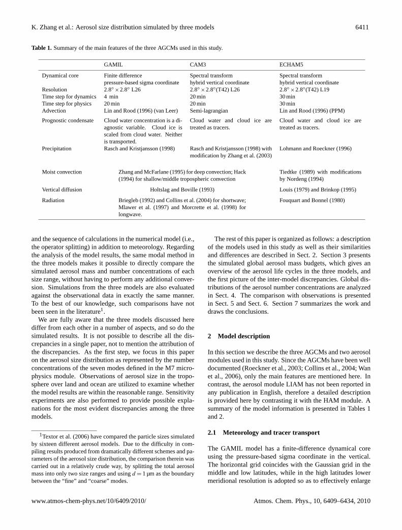
Table 1. Summary of the main features of the three AGCMs used in this study.

GAMIL CAM3 ECHAM5

Dynamical core Finite difference Spectral transform Spectral transformpressure-based sigma coordinate hybrid vertical coordinate hybrid vertical coordinate

Resolution 2.8◦×2.8◦ L26 2.8◦

×2.8◦(T42) L26 2.8◦×2.8◦(T42) L19

Time step for dynamics 4 min 20 min 30 minTime step for physics 20 min 20 min 30 minAdvection Lin and Rood(1996) (van Leer) Semi-lagrangian Lin and Rood(1996) (PPM)

Prognostic condensate Cloud water concentration is a di-agnostic variable. Cloud ice isscaled from cloud water. Neitheris transported.

Cloud water and cloud ice aretreated as tracers.

Cloud water and cloud ice aretreated as tracers.

Precipitation Rasch and Kristjansson(1998) Rasch and Kristjansson(1998) withmodification byZhang et al.(2003)

Lohmann and Roeckner(1996)

Moist convection Zhang and McFarlane(1995) for deep convection;Hack(1994) for shallow/middle tropospheric convection

Tiedtke (1989) with modificationsby Nordeng(1994)

Vertical diffusion Holtslag and Boville(1993) Louis (1979) andBrinkop (1995)

Radiation Briegleb(1992) andCollins et al.(2004) for shortwave;Mlawer et al. (1997) and Morcrette et al.(1998) forlongwave.

Fouquart and Bonnel(1980)

and the sequence of calculations in the numerical model (i.e.,the operator splitting) in addition to meteorology. Regardingthe analysis of the model results, the same modal method inthe three models makes it possible to directly compare thesimulated aerosol mass and number concentrations of eachsize range, without having to perform any additional conver-sion. Simulations from the three models are also evaluatedagainst the observational data in exactly the same manner.To the best of our knowledge, such comparisons have notbeen seen in the literature1.

We are fully aware that the three models discussed herediffer from each other in a number of aspects, and so do thesimulated results. It is not possible to describe all the dis-crepancies in a single paper, not to mention the attribution ofthe discrepancies. As the first step, we focus in this paperon the aerosol size distribution as represented by the numberconcentrations of the seven modes defined in the M7 micro-physics module. Observations of aerosol size in the tropo-sphere over land and ocean are utilized to examine whetherthe model results are within the reasonable range. Sensitivityexperiments are also performed to provide possible expla-nations for the most evident discrepancies among the threemodels.

1Textor et al.(2006) have compared the particle sizes simulatedby sixteen different aerosol models. Due to the difficulty in com-piling results produced from dramatically different schemes and pa-rameters of the aerosol size distribution, the comparison therein wascarried out in a relatively crude way, by splitting the total aerosolmass into only two size ranges and usingd = 1 µm as the boundarybetween the “fine” and “coarse” modes.

The rest of this paper is organized as follows: a descriptionof the models used in this study as well as their similaritiesand differences are described in Sect.2. Section3 presentsthe simulated global aerosol mass budgets, which gives anoverview of the aerosol life cycles in the three models, andthe first picture of the inter-model discrepancies. Global dis-tributions of the aerosol number concentrations are analyzedin Sect.4. The comparison with observations is presentedin Sect.5 and Sect.6. Section7 summarizes the work anddraws the conclusions.

2 Model description

In this section we describe the three AGCMs and two aerosolmodules used in this study. Since the AGCMs have been welldocumented (Roeckner et al., 2003; Collins et al., 2004; Wanet al., 2006), only the main features are mentioned here. Incontrast, the aerosol module LIAM has not been reported inany publication in English, therefore a detailed descriptionis provided here by contrasting it with the HAM module. Asummary of the model information is presented in Tables1and2.

2.1 Meteorology and tracer transport

The GAMIL model has a finite-difference dynamical coreusing the pressure-based sigma coordinate in the vertical.The horizontal grid coincides with the Gaussian grid in themiddle and low latitudes, while in the high latitudes lowermeridional resolution is adopted so as to effectively enlarge

www.atmos-chem-phys.net/10/6409/2010/ Atmos. Chem. Phys., 10, 6409–6434, 2010


Table 2. Summary of the main components of the two aerosol modules used in this study.

LIAM HAM

EmissionSU, BC, POM AEROCOM AEROCOMSS Guelle et al.(2001), Smith and Harrison

(1998) andGong(2003)Guelle et al.(2001), Smith and Harrison(1998) andMonahan et al.(1986)

DU Zender et al.(2003) Tegen et al.(2002)Sulfur chemistry Barth et al.(2000) Feichter et al.(1996)Gas oxidants IMAGE monthly mean output of OH,

NO3, HO2

MOZART monthly mean output of OH,H2O2, O3, HO2, NO3

Dry deposition Prescribed deposition velocities for gases(Feichter et al., 1996); Zhang et al.(2001)for aerosols

Ganzeveld and Lelieveld (1995);Ganzeveld et al.(1998)

Sedimentation Seinfeld and Pandis(1998) with smallertime step for large particles

Seinfeld and Pandis(1998) with CFL sta-bility limitation

Wet deposition Similar to HAM, except for below-cloudscavenging (see text)

Herry’s Law for gases in-cloud; below-cloud scavenging and re-evaporation ofaerosols

Aerosol microphysics M7 module M7 moduleNumber of advective chemical tracers 25 aerosols and 4 precursor gases 25 aerosols and 3 precursor gases

the zonal grid size and reduce the computational instabilityin the Polar Regions. ECHAM5 and the Eulerian version ofCAM3 both utilizes the spectral transform method for hor-izontal discretization. The grid-point calculations are per-formed on the Gaussian grid. The hybridp-σ vertical coor-dinate is used in both spectral models although the layers arelocated differently. In this study, simulations with the threemodels are conducted at similar spatial resolutions (see Ta-ble1). Large-scale tracer transport in GAMIL and ECHAM5is handled by the Flux Form Semi-Lagrangian (FFSL) algo-rithm (Lin and Rood, 1996). In CAM3 the semi-Lagrangianmethod proposed byWilliamson and Rasch(1989) is em-ployed. In order to ensure computational stability and at thesame time preserve consistency between tracer transport andthe continuity equation, GAMIL uses a relatively short timestep (4 min) for the dynamical core and the transport scheme.The time steps used in CAM3 and ECHAM5 are 20 min and30 min respectively.

The physics parameterizations in GAMIL originates fromCAM2 and is therefore similar to CAM3. The major dif-ferences reside in the treatment of cloud condensed water.In GAMIL the cloud water and cloud ice concentrations arediagnosed and neither is transported, while in CAM3 theyare both treated as advective tracers. Details of the physicsparameterizations in the ECHAM5 model differ significantlyfrom the CAM package. The main processes that are directlyrelated to aerosol simulation include the cumulus convec-tion, cloud, precipitation and the boundary layer processes.A brief comparison of the physics packages is presented inTable1. For physical parameterizations, GAMIL and CAM3use a time step of 20 min, while ECHAM5 uses 30 min timestep.

2.2 The microphysics module M7

As already mentioned in the introduction, both LIAM andHAM employ the M7 module (Vignati et al., 2004) foraerosol microphysics. The aerosol composition consideredincludes sulfate, black carbon, particulate organic matter,sea salt and dust. Different composition can be internallyand/or externally mixed. The aerosol size spectrum is repre-sented by a superposition of several log-normal modes, eachof which has fixed mode boundaries and standard deviationand varying median radius. According to the particle sizeand solubility, the whole aerosol population is divided intoseven modes shown in Table3. Each individual mode is rep-resented by its total particle number, and the mass of differ-ent compositions within this mode, which are all treated asadvective tracers (Table3).

The processes considered in the M7 module include nu-cleation, coagulation, sulfuric acid condensation and wateruptake. We do not describe the details here and refer readersto the paper byVignati et al.(2004). Note that there are twoparameterizations available in M7 for calculating the forma-tion of new sulfuric acid-water droplets: one byVehkamaki(2002) and the other byKulmala et al.(1998). Vignati et al.(2004) have pointed out that theVehkamaki(2002) scheme isvalid in broader ranges of temperatures and humidity, thus allsimulations in this study are conducted with theVehkamaki(2002) parameterization.



Table 3. The log-normal modes in the M7 module and the related sources and sinks of aerosol mass and particle number.rd stands for thedry radius of the aerosol particle;σ denotes the geometric standard deviation of the size distribution function. “N ” and “M” in the thirdcolumn stand for the number and mass concentrations, respectively. Their subscripts indicate the corresponding mode. The superscript of“M” indicate the composition. Small circles indicate that a certain tracer is affected by a specific process.

Mode andrd (µm) σ TracersSources and sinks

primaryemission

nucleation condensation coagulation dry de-position

wet de-position

sedimentation

nucleation soluble Nns ◦ ◦ ◦ ◦

< 0.005 1.59 MSUns ◦ ◦ ◦ ◦

Nks ◦ ◦ ◦ ◦ ◦

Aitken soluble MBCks ◦ ◦ ◦ ◦

0.005–0.05 1.59 MPOMks ◦ ◦ ◦ ◦ ◦

MSUks ◦ ◦ ◦ ◦ ◦

Nas ◦ ◦ ◦ ◦ ◦ ◦

accumulation soluble MBCas ◦ ◦ ◦ ◦ ◦

MPOMas ◦ ◦ ◦ ◦ ◦ ◦

0.05–0.5 1.59 MSUas ◦ ◦ ◦ ◦ ◦ ◦

MSSas ◦ ◦ ◦ ◦ ◦ ◦

MDUas ◦ ◦ ◦ ◦ ◦

Ncs ◦ ◦ ◦ ◦ ◦ ◦

MBCcs ◦ ◦ ◦ ◦ ◦

coarse soluble MPOMcs ◦ ◦ ◦ ◦ ◦ ◦

> 0.5 2.00 MSUcs ◦ ◦ ◦ ◦ ◦ ◦

MSScs ◦ ◦ ◦ ◦ ◦ ◦

MDUcs ◦ ◦ ◦ ◦ ◦

Aitken insolubleNki ◦ ◦ ◦ ◦ ◦

MBCki ◦ ◦ ◦ ◦ ◦

0.005–0.05 1.59 MPOMki ◦ ◦ ◦ ◦ ◦

accumulation insoluble Nai ◦ ◦ ◦ ◦ ◦ ◦

0.05–0.5 1.59 MDUai ◦ ◦ ◦ ◦ ◦ ◦

coarse insoluble Nci ◦ ◦ ◦ ◦ ◦ ◦

> 0.5 2.00 MDUci ◦ ◦ ◦ ◦ ◦ ◦

2.3 Chemistry

For an aerosol-climate model, it would be advantageous tohave complex gas chemistry within the model system so asto allow for full interactions between the gas oxidants and theaerosols. However, this would lead to a significant increasein the required computational resources. In this study onlythe sulfur chemistry is interactively simulated.

The LIAM and HAM aerosol modules use the sulfurchemistry schemes proposed byBarth et al.(2000) andFe-ichter et al.(1996), respectively. Both schemes have consid-ered the gas phase oxidation of dimethyl sulfide (DMS) andsulfur dioxide (SO2), reaction of DMS with nitrate radicals(NO3), as well as aqueous phase oxidation of SO2 by H2O2and O3, although the reaction rate constants are slightly dif-ferent. The mixing ratio of DMS, SO2 and sulfate (SO2−

4 )are prognostic variables in both modules. The mixing ratioof H2O2 is also predicted in LIAM but not in HAM.

Sulfuric acid gas (H2SO4) produced by gas phase chem-istry can either condense on existing particles or form newparticles through particle nucleation. These two processesare handled in the M7 module introduced above. Sulfate pro-duced in the aqueous chemistry is distributed to particles ofthe soluble accumulation mode and coarse mode accordingto the respective number concentration (Stier et al., 2005).This calculation is done in the sulfur chemistry scheme.

As for the other related oxidants, OH, O3, NO3 and HO2concentrations needed in LIAM are prescribed using three-dimensional monthly means obtained from the IntermediateModel of Global Evolution of Species (IMAGES,Muller andBrasseur, 1995). In the HAM module, OH, H2O2, NO2 andO3 concentrations are prescribed using monthly means givenby the comprehensive Model of Ozone And Related Tracers(MOZART, Horowitz et al., 2003).



It is worth noting that the NO3 concentration in the HAMmodule is not prescribed but calculated assuming a steadystate between the production terms (i.e. depletion ofN2O5)and loss terms (reacts with NO2 and DMS) (Feichter et al.,1996). Furthermore, the methane sulfuric acid (MSA) pro-duced from the oxidation of DMS is assumed to occur assulfuric acid in HAM. In the LIAM package the further con-version of MSA is ignored.

2.4 Emission

Global emission information is needed as an external forc-ing for the simulated aerosol composition and for precursorgases. In the present study we follow the experiment speci-fications of the Aerosol inter-Comparison project AeroCom(http://nansen.ipsl.jussieu.fr/AEROCOM/).

Due to the fact that no recommendation has been made foroxidant fields (Dentener et al., 2006), different data sets areused in the LIAM and HAM modules as already described inSect.2.3. In HAM the oceanic DMS emission is calculatedonline (Stier et al., 2005), while the terrestrial biogenic DMSemissions are prescribed following Pham et al. (1995). InLIAM both are prescribed using the data provided by Aero-Com (Dentener et al., 2006). For SO2, sulfate, black carbonand the particulate organic matter, the emission rate and in-jection height are available from AeroCom (Dentener et al.,2006) at 1◦

×1◦ (longitude×latitude) resolution. The origi-nal data are mapped to the model grids using area-weightedinterpolation.Dentener et al.(2006) have also specified thesize distribution for the emissions. Since the recommendedstandard deviations differ from the values used in M7 mod-ule, the mode radius has been adapted to the (M7) modelparameters (Stier et al., 2005). The partitioning of aerosolemissions among different modes is summarized in Table4.

Sea salt particles are generated at the ocean’s surface bythe bursting of entrained air bubbles induced by wind stress(Monahan et al., 1986). Experimental investigations have in-dicated that the injection of sea salt into the atmosphere de-pends strongly on the meteorological conditions at the seasurface (Gong et al., 1997). In numerical models, genera-tion of sea salt particles is usually parameterized by empir-ical functions of the droplet size and the 10-m wind speed.Previous studies (e.g.,Guelle et al., 2001) have shown thatthe scheme ofMonahan et al.(1986) works well for particleradius below 4 µm, and the formulation ofSmith and Harri-son(1998) is most appropriate for particles larger than 4 µm.In the HAM module, the two source functions are mergedsmoothly within the size range of 2–4 µm, and fitted into theaccumulation mode and coarse mode. In LIAM, theSmithand Harrison(1998) scheme is used for particles larger than4 µm, theMonahan et al.(1986) scheme is used for the sizerange 0.2–4 µm, and the modification byGong(2003) is em-ployed for radii below 0.2 µm to avoid the overestimates re-sulting from theMonahan et al.(1986) scheme.

Emission of dust is computed online in both aerosol mod-ules according to the surface land types, 10-m wind andother atmospheric boundary layer properties. HAM uses thescheme proposed byTegen and Lacis(1996), calculates theemission flux from 192 internal size classes, then fit theminto the insoluble accumulation and coarse modes; in LIAM,the modal algorithm ofZender et al.(2003) is adapted bymapping the original source size distribution into the insolu-ble accumulation and coarse modes, resulting in about 96%of the emitted particle mass attributed to the coarse mode.

2.5 Dry deposition

Dry deposition is an important sink of aerosols and tracegases in the atmosphere. There are two main contributingmechanisms: the turbulent dry deposition happening near theEarth’s surface and the gravitational settlement (i.e. sedimen-tation) which occurs within the whole vertical domain of theatmosphere. Both mechanisms can be described by a generalformulation

Fi = CiρaVi , (1)

which indicates that for a particular speciesi, the dry depo-sition fluxFi is proportional to the species’ densityCiρa andthe deposition velocityVi . The central task of the depositionparameterization is to find out an appropriate expression forVi .

The removal rate of aerosols from the atmosphere viadry deposition is closely related to the size of the particles.In many previous studies, especially those using the bulkmethod, the deposition velocity is usually linked to someprescribed (fixed) values of particle size. The modal ap-proach adopted by the M7 module allows for varying sizespectra, therefore both in HAM and in LIAM, the mode ra-dius derived from the predicted number and mass concentra-tions is used to represent the particle size of aerosols. More-over, due to the fact that the mass and number concentra-tions are treated as separate tracers, the size spectra in thetwo aerosol modules are interactively affected by the deposi-tion processes.

As will be demonstrated later, some evident differenceshave been detected in the simulation results from the threeaerosol-climate model systems used in this study, which isattributable to the deposition processes. In order to facilitatelater analysis, crucial details of the parameterization schemesare summarized and compared below.

2.5.1 Turbulence dry deposition

The turbulent dry deposition affects both the trace gases andaerosols. The deposition velocity is usually computed usingthe big leaf approach asVDep=R−1 with R being the param-eterized resistance.




Table 4. Partitioning of the aerosol emissions among different modes. The small circles in the last two rows denote online calculation.

Composition Emission typeInsoluble modes Soluble modes

Aitken accumulation coarse Aitken accumulation coarse

Black carbonbio-fuel 100%fossil fuel 100%biomass burning 100%

Particulateorganicmatter

fossil fuel 100%bio-fuel 35% 65%biogenic 35% 32.5% 32.5%biomass burning 35% 65%

Sulfate

off-road 50% 50%road transport 50% 50%domestic 50% 50%international shipping 50% 50%industry 50% 50%power plant 50% 50%biomass burning 50% 50%continuous volcano 50% 50%eruptive volcano 50% 50%

Sea salt online calculation ◦ ◦

Dust online calculation ◦ ◦

For gaseous tracers, the scheme ofGanzeveld andLelieveld (1995) andGanzeveld et al.(1998) is used in theHAM module. The first contributor to resistanceR is theaerodynamic resistanceRa determined by atmospheric sta-bility and friction velocity (calculated by the boundary layerscheme in the GCM), which are in turn functions of thevertical gradient of temperature and momentum near theEarth’s surface; the second contributor, quasi-laminarbound-ary layer resistanceRb, is determined by kinematic viscosityof air (a function of temperature), friction velocity, and someempirical parameters. The third contributor,surface resis-tanceRs , is prescribed for most trace gases, with the onlyexception that the SO2 soil resistance is computed from soilpH, relative humidity, surface temperature, and the canopyresistance (Stier et al., 2005). The total resistance is thengiven as the sum of these three contributors.

This online calculation provides a consistent depositionvelocity in the sense that it changes instantaneously withmodel meteorology and the underlying surface character-istics. On the other hand, the study byFeichter et al.(1996) showed that the dry deposition velocities prescribedby Langner and Rodhe(1991) for different chemical con-stituents and surface types work well in simulation of thetropospheric sulfur cycle. In the LIAM model we follow thework of Feichter et al.(1996) and use the same prescribedvalues for gaseous sulfur species and precursors.

As for aerosol particles, both the HAM and LIAM mod-ules use the big leaf method withR = Ra +Rs . A detaileddescription of the resistance calculation used in HAM can

be found inKerkweg et al.(2006). The parameterizationscheme for aerosol particles used in LIAM follows the workof Zhang et al.(2001). Since the actual formulas are ratherlengthy, we only provide a brief summary here:

– The aerodynamic resistanceRa in both modules are cal-culated in the same way as for the trace gases in HAM.

– The surface resistanceRs depends on the particle sizeand the surface collection efficiency. The latter is deter-mined by the atmospheric conditions and the propertiesof the Earth’s surface.

– When calculating the surface collection efficiency, bothmodules have considered the Brownian diffusion, im-paction and interception, of which control variables arethe Schmidt number, the Stokes number and particle ra-dius, respectively. On the other hand, HAM and LIAMdiffer in the formulation details and in the empirical pa-rameters.

– Regarding particle radius, the mass mean and numbermedian radius of each mode are used for calculatingRs of aerosol mass and number concentrations, respec-tively.

– The dry deposition flux of nucleation mode particles isvery small and thus ignored in both modules.



2.5.2 Sedimentation

Sedimentation affects on aerosol particles throughout thewhole vertical domain of the model atmosphere. The sedi-mentation velocities in HAM and LIAM are both calculatedbased on the Stokes theory (see, e.g., p. 465 inSeinfeld andPandis, 1998), which describes the dynamical movement ofa singleparticle. Since the modal representation in M7 eachmode includes particles of different sizes, the mass (number)medianradius is used in the calculation of sedimentation ve-locity of aerosol mass (number), and then the Slinn correc-tion (Slinn and Slinn, 1980) is used to get the sedimentationvelocity of a log-normal aerosol size distribution with a givenstandard deviation.

To avoid violation of the Courant-Friedrich-Lewy stabilitycriterion, the sedimentation velocity is limited toV < 1z

1tin

HAM, where1z is the layer thickness (in meters) and1t isthe model time step (Stier et al., 2005). In LIAM, we taketwo successive time steps (1t/2 each) when updating thesoluble and insoluble coarse modes, so as to preserve com-putational stability and achieve higher accuracy.

It is worth noting that although the mass concentrations ofdifferent composition in the same soluble mode are treatedas separate tracers, they are assumed to be internally mixed.For each mode, a single mass median radius is derivedfrom the number concentration and thetotal mass concen-tration, and used subsequently in the calculation of turbu-lent/sedimentation velocity. Therefore the mass concentra-tions in each mode – as different tracers – share the samedeposition velocities.

2.6 Wet deposition

Wet deposition parameterization simulates the loss of tracegases and aerosols caused by cloud formation (i.e. the in-cloud scavenging) and precipitation (the so-called below-cloud scavenging), as well as release of these tracers backinto the atmosphere due to the evaporation of rain droplets.All these three processes are considered both in HAM and inLIAM. The impact on gases and aerosols are treated differ-ently. For gases, the solubility in cloud water and removalby precipitation are calculated according to the Henry’s law(see, e.g.,Seinfeld and Pandis, 1998). As for aerosols, thefraction of the total amount that is involved in cloud forma-tion is prescribed according to the size and solubility of eachaerosol type (see Table 3 inStier et al., 2005). In reality thein-cloud loss is caused by the activation process which con-verts aerosol particles into cloud droplets. However, the pa-rameterization of activation is not explicitly included in themodel versions used in the present study. The precipitationformation rate is further used to convert activated aerosols toprecipitation phase. Therefore the resulting in-cloud aerosolloss depends strongly on the strength and distribution of pre-cipitation predicted by the hosting GCM. The formulation ofthe in-cloud scavenging in LIAM is essentially the same as in

HAM, although the parameters have been slightly scaled soas to provide reasonable deposition rates (according to simu-lated total wet deposition flux and aerosol lifetime).

Aerosols below precipitating clouds are subject to removalfrom the atmosphere by rain droplets. The resulting concen-tration tendency is assumed to be proportional to the pre-cipitation rate and area, and the collection efficiency. Thesize-dependent collection efficiency for rain and snow fol-lows Seinfeld and Pandis(1998). LIAM and HAM only dif-fer slightly in the calculation of precipitation area.

3 Model setup and simulated global mean mass budgetand lifetime

Climate simulations are conducted using the three aerosol-climate models mentioned above, each proceeding 3 modelyears. The meteorological fields are initialized using the out-put of a long-term simulation with the same model but with-out aerosols. The sea surface temperature and sea ice con-centration (as external forcing) are the 1979–2001 multi-yearmean monthly average. The initial aerosol concentrations arezero. Typically the aerosol burden increases to its normal av-erage values within less than one model year. Thus we cal-culate the diagnostics based on the monthly average outputof the last two model years of the simulations.

Before going into details of the simulated aerosol size dis-tributions, we first present an overall picture of the aerosollife cycles in the three models by showing in Tables5 and6 the globally averaged annual mean mass budget and lifetimes of the five aerosol types. The corresponding valuesin some other models mentioned inLiu et al. (2005) are pre-sented in the rightmost columns for comparison. To facilitateanalysis, the precursors of sulfate are also included.

The first message from the two tables is that regardingglobal mean burdens, results from the three models are quitesimilar for all the five aerosol types. The ECHAM5-HAMresults shown here at T42L19 resolution are also very closeto the T63L31 nudged simulation inStier et al.(2005)2.On the other hand, discrepancies between models exist inthe contribution from specific process. For sulfate and car-bonous aerosols, the differences between GAMIL-LIAM andCAM3-LIAM are evidently much smaller than between ei-ther of them and ECHAM5-HAM. This suggests that globaland annual mean budgets of these species are highly sensitiveto the parameterization schemes of the aerosol-related phys-ical (e.g. transport and deposition) and chemical processes.

The sulfate aerosol burdens simulated by the LIAM andHAM modules turn out to have similar dynamical equilibri-ums which result from sulfur cycles with significantly differ-ent strengths. This can been seen from the different lifetimes(see the “SO2−

4 particle” part of Table5). Both the source and

2An exception here is dust, for which it is already known that theemission flux in nudged simulations is significantly smaller than inclimatological runs (Timmreck and Schulz, 2004).



Table 5. Annual mean global sulfur budget obtained in this study and from the literature.

GAMIL CAM3 ECHAM5 from-LIAM -LIAM -HAM Liu et al. (2005)

SO2−

4 particleBurden (Tg S) 0.72 0.75 0.75 0.53–1.07

Sources (Tg S yr−1) Total 59.2 61.7 75.6Primary emissions 1.76 1.77 1.78 0–3.5Nucleation 0.044 0.046 0.044H2SO4 condensation 6.1 7.4 25.0 6.1–22.0Aqueous oxidation 51.3 52.5 48.8 24.5–57.8

Sinks (Tg S yr−1)Total 60.9 62.4 75.8Dry deposition 2.8 2.9 2.5

} 3.9–18.0Sedimentation 1.3 1.1 1.7Wet deposition 56.8 58.4 71.6 34.7–61.1

Lifetime (days) 4.4 4.5 3.6 3.9–6.8

Sulfuric acid gasBurden (Tg S) 0.00040 0.00052 0.00060Sources (Tg S yr−1)

Total 6.2 7.4 25.1SO2 + OH (gas) 6.2 7.4 22.5DMS + OH (gas) – – 2.6

Sinks (Tg S yr−1)Total 6.1 7.3 25.1Nucleation 0.044 0.046 0.044H2SO4 condensation 6.1 7.3 25.0Dry deposition 0.0006 0.0014 0.009

Lifetime (days) 0.023 0.030 0.010

SO2Burden (Tg S) 0.34 0.35 0.58 0.2–0.69Sources (Tg S yr−1)

Total 84.9 85.2 94.4Emissions 68.7 68.9 71.7DMS + OH (gas) 12.0 12.0 17.5

} 10.0–25.6DMS + NO3 (gas) 4.2 4.3 5.2

Sinks (Tg S yr−1)Total 84.9 85.3 92.6SO2 + OH (gas) 6.2 7.4 22.5 6.1–22.0Sink in aqueous chem. 51.3 52.3 48.8 24.5–57.8Dry deposition 26.8 24.5 16.8 16.0–55.0Wet deposition 0.61 0.65 4.5 0–19.9

Lifetime (days) 1.0 0.95 2.2 0.6–2.6

DMSBurden (Tg S) 0.093 0.087 0.085 0.02–0.15Source (Tg S yr−1)

Emissions 18.2 18.2 25.4 10.7–26.1Sinks (Tg S yr−1)

DMS + OH (gas) 14.1 14.0 17.5DMS + NO3 (gas) 4.2 4.3 5.2

Lifetime (days) 1.9 1.7 1.3 0.5–3.0



loss rates in ECHAM5-HAM are more than 30% larger thanin the other two models, which can be attributed mainly tothe stronger H2SO4 condensation (source) and stronger wetdeposition (sink). Compared to the other models results col-lected inLiu et al.(2005), it seems that the condensation ratein ECHAM5-HAM is higher than the other models, while thevalues in the two models using LIAM are among the lowest(see the rightmost column in Table5).

The strong condensation in ECHAM5-HAM is directly re-lated to the high H2SO4 production from the oxidation ofSO2 by OH. According to the numbers listed in Table5 andthe comparison between the parameterization schemes in theHAM and LIAM modules, there can be two immediate rea-sons for the different H2SO4 productions: 1) stronger SO2production from DMS and weaker dry deposition of the SO2gas in ECHAM5-HAM, which may have lead to higher SO2burden; 2) differences in the concentrations of the oxidantswhich are prescribed using different data sets.

In order to quantify the contribution from these fac-tors, several sensitivity tests are performed using ECHAM5-HAM:

– Experiment Ia, in which the turbulent dry depositionin HAM is replaced by the parameterization in LIAM.As expected, the dry deposition rate in ECHAM5-HAMis enhanced to a level similar to the other two models,the oxidation of SO2 is weakened, and the H2SO4 con-densation rate is reduced from 25.0 to 21.9 Tg S yr−1

(by 12.4%). Understandably, the SU burden is also de-creased.

– Experiment Ib, in which the DMS emission is scaleddown to the global and annual mean prescribed by Ae-roCom (i.e., from 25.4 to 18.2, see Table5). This leadsto reduced SO2 production, and eventually a 6.4% de-crease of the condensation of H2SO4 (i.e., from 25.0 to23.4). Like in the first experiment, the SU burden is alsodecreased.

– Experiment II, in which the oxidant concentrations areprescribed using the IMAGES model data as in the othertwo models. In this simulation more SO2 are con-sumed in the aqueous phase oxidation and less in thegas phase reactions, but the total amount remains almostunchanged. Although the condensation rate is reducedto 22.5 Tg S yr−1, there is no significant change in eitherthe burden or the lifetime of the SU aerosol.

– Experiment III, in which the three modifications aboveare combined in one simulation to take into account theinteraction and nonlinearity. It turns out that in termsof H2SO4 condensation rate, the decrease is close to thesum of the changes in the previous three experiments.Although reduced to 17.6 Tg S yr−1, it is still more thantwice the values in the other two models.

These tests suggest that the large differences of the H2SO4production in the three models must have resulted from otherreasons than the dry deposition of SO2, DMS emission,and the oxidants. Possibilities include the chemical reac-tion schemes, the related meteorological conditions (such ascloud liquid content and cloud cover), and the sequence ofcalculating the various processes (including the gas/aqueousphase reactions and deposition processes) within the sulfurchemistry scheme. Which of these plays the major role isnot yet clear. We will leave the further analysis in the futureresearch.

The dramatic differences in the H2SO4 condensation ratemay lead to significant discrepancies in the simulated sizedistributions. So as to investigate the impact, anothersensitivity experiment, referred to as “EXP-60P”, is per-formed with ECHAM5-HAM. Here we manually reducedthe H2SO4 production to 60% of the original values, andapply the same scaling factor to the wet deposition coeffi-cients. The simultaneous reduction of the source and sinkof SU does not affect the burden, but increases the SU life-time to 4.1 days. Other results from this simulation will bediscussed in the next section.

Regarding BC and POM, the burdens and total sources andsinks strengths are very similar in the three models (Table6).The values are also well within the range given by previousstudies (see the last column in Table6) and by the AeroCommodels. The main difference between the three models is therelative contribution from the wet and dry deposition to thereduction rate.

Sea salt has a relatively simple life cycle compared to theother aerosol types, and is more sensitive to the 10-m windwhich determines its emission process. The differences inour simulations (Table6) can be regarded as indication ofdifferences in the emission schemes in use and the discrep-ancies in model meteorology in the near surface layers. Fur-ther details are presented in the next section. As for dust, theemission rate depends additionally on the underlying surfacecharacteristics (which are typically prescribed using externaldata), as well as on the parameterization scheme of mobi-lization. Since these data and schemes are highly empiricaland consequently associated with large uncertainties, we listthe dust budget in Table6 for completeness but do not makefurther quantitative comparison.

4 Global distribution of aerosol number concentration

In this section we present and inter-compare the simulatedannual mean number concentrations of all the seven modesresolved by the M7 module. In the figures the concentrationis given as number of particles per cubic centimeter at thestandard atmospheric state (1013.25 hPa, 273.15 K).



Table 6. Annual mean global BC, POM, SS, DU budgets obtained in this study and from the literature.

GAMIL CAM3 ECHAM5 from-LIAM -LIAM -HAM Liu et al. (2005)

Black carbonBurden (Tg) 0.13 0.13 0.11 0.12–0.29Sources (Tg yr−1)

Emissions 7.7 7.7 7.7Sinks (Tg yr−1)

Total 7.6 7.6 7.8Dry deposition 0.87 1.1 0.71

}1.6–4.6Sedimentation 0.02 0.02 0.03Wet deposition 6.7 6.2 7.1 7.8–13.7

Lifetime (days) 6.2 6.2 5.2 3.3–8.4

POMBurden (Tg) 1.2 1.1 0.93 0.95–1.8Sources (Tg yr−1)

Emissions 65.8 65.8 66.6Sinks (Tg yr−1)

Total 65.9 65.8 66.0Dry deposition 5.8 7.2 5.7

}11.3–29.8Sedimentation 0.11 0.10 0.21Wet deposition 60.0 58.5 60.1 60.1–113.3

Lifetime (days) 6.3 6.2 5.1 3.2–6.4

Sea saltBurden (Tg) 12.9 14.9 11.3 3.4–12.0Sources (Tg yr−1)

Emissions 8366 11 785 6615 1010–8076Sinks (Tg yr−1)

Total 8389 11 845 6650Dry deposition 1432 2586 1680

}940–7450Sedimentation 3730 4454 1800Wet deposition 3227 4805 3170 74–2436

Lifetime (days) 0.57 0.46 0.62 0.19–0.99

DustBurden (Tg) 13.6 13.9 16.8 4.3–35.9Sources (Tg yr−1)

Emissions 1052 1201 1378 820–5102Sinks (Tg yr−1)

Total 1075 1210 1389Dry deposition 36.1 61 120

}486–4080Sedimentation 325 437 550Wet deposition 714 712 719 183–1027

Lifetime (days) 4.7 4.2 4.4 1.9–7.1

4.1 Nucleation mode and soluble Aitken mode

The first two rows in Fig.1 display the zonal and annualmean number concentrations of the nucleation mode and thesoluble Aitken mode simulated by the three models. In bothLIAM and HAM, particles of the nucleation mode are gen-erated exclusively from the neutral binary nucleation. Strongconversion of the sulfuric acid gas to particles results from

high sulfuric acid concentration, high relative humidity andlow temperature. Thus the upper troposphere is the most fa-vorable region, as can be seen in the vertical cross sections(Fig. 1, first row). The soluble Aitken mode particles in M7are internal mixtures of sulfate, black carbon and organic car-bon. In the middle and upper troposphere, the most impor-tant source of Aitken mode particles is the condensation ofsulfuric acid gas on nucleation mode particles.



Fig. 1. Zonal and annual mean aerosol number concentrations of the four soluble modes (from top to bottom) simulated by GAMIL-LIAM(left column), CAM3-LIAM (middle column) and ECHAM5-HAM (right column). The unit is number of particles per cubic centimeter atthe standard atmospheric state (1013.25 hPa, 273.15 K).

Regarding the nucleation mode, the three model simula-tions agree reasonably well in the vertical distribution andthe magnitude of the number concentration. This is consis-tent with the similar global and annual mean nucleation rates(see the first block of Table5). The most evident differenceis the higher concentrations near the tropical upper tropo-sphere in the two models using LIAM. As for the solubleAitken mode, all three models agree that the tropical regionsare associated with relatively high concentrations, althoughthe actual values differ significantly.

As mentioned in the previous section, the sensitivity ex-periment EXP-60P has been conducted with ECHAM5-HAM, in which the H2SO4 yields due to the oxidation ofSO2 is scaled down to 60% of the original values. Theconsequence is that near the tropical upper tropospherethe nucleation mode number concentration is increased dueto slower growth of nucleation mode particles, and thusthe Aitken mode number concentration is considerably de-creased (Fig.2, right column). In another experiment inwhich the H2SO4 yields in CAM3-LIAM are doubled, theAitken mode number concentration increases and the pattern

becomes much more similar to the ECHAM5-HAM result(Fig. 2, left column). These two experiments indicate thatthe condensation of H2SO4 plays a major role in the particlegrowth in the aforementioned region, and can lead to largediscrepancies among models in the number concentrationsof the nucleation and soluble Aitken modes.

Near the surface layers, nucleation mainly happens in thehigh-latitude continental areas. As expected, the high num-ber concentrations in ECHAM5-HAM and GAMIL-LIAMare high over Antarctica and North Eurasia (first row inFig. 3) are consistent with expectation. The lower concen-tration in GAMIL-LIAM over Greenland, Siberia and north-west part of North America is related to the warm bias in win-ter (not shown). In CAM3-LIAM, the high concentrationsfrom 45◦ N are missing, probably also due to the tempera-ture bias, since the 2-m temperature is typically associatedwith a positive bias of 2 to 12◦C3. The higher concentrationsin ECHAM5-HAM seem partly attributable to the abundant

3Figure available from the CAM 3.0 Simulation Page:http://www.ccsm.ucar.edu/models/atm-cam/sims/cam3.0/cam20 2 dev59/cam20 2 dev59-obs/set56/set5DJF TREFHT


http://www.ccsm.ucar.edu/models/atm-cam/sims/cam3.0/cam2_0_2_dev59/cam2_0_2_dev59-obs/set5_6/set5_DJF_TREFHT_CRU_obsc.png



Fig. 2. Zonal and annual mean aerosol number concentrations of the nucleation mode (upper row) and Aitken soluble mode (bottom row)simulated by CAM3-LIAM (left colomn) and ECHAM5-HAM (right column) in sensitivity tests. The unit is number of particles percubic centimeter at the standard atmospheric state (1013.25 hPa, 273.15 K). In the CAM3-LIAM simulation the H2SO4 yields are doubledcompared to the control experiment. In the ECHAM5-HAM simulation (referred to as “EXP-60P” in the text), both the H2SO4 yields andthe wet deposition coefficients are scaled down to 60% of the original values.

H2SO4. In the EXP-60P simulation the nucleation mode con-centration is generally lower from 40◦ latitudes pole-ward,both over land and over the ocean (not shown).

The soluble Aitken mode particles near the Earth’s sur-face mainly come from natural and anthropogenic emissionsand aging of the insoluble particles. Aging itself is a phys-ical process in LIAM and HAM, caused by condensationand the coagulation of insoluble aerosols with soluble par-ticles. These processes, however, are closely related withthe sulfur cycle. From the second row of Fig.3 it is clearthat ECHAM5-HAM produces more soluble Aitken modeparticles. Over the mid-latitude continents in the NorthernHemisphere, the higher number concentrations are probablya result of stronger aging. Over the Southern Oceans, the ox-idation of DMS leads to relatively high sulfuric acid concen-tration. Sulfur chemistry and aerosol microphysics (nucle-ation, condensation and coagulation) thus become the mainsource of the small soluble particles. ECHAM5-HAM fea-tures stronger DMS emission (see the previous section andthe last block of Table5); additionally, in the sulfur chemistryscheme, the MSA produced from DMS is assumed to occuras sulfuric acid. In the two models using LIAM the conver-sion from MSA to sulfuric acid is simply ignored. Sensitiv-ity test shows that if the same is done in ECHAM5-HAM,the near surface concentration of the soluble Aitken particleswill be evidently reduced over the circumpolar trough andAntarctica (Fig.4).

CRU obsc.png

4.2 Soluble accumulation mode and soluble coarsemode

In contrast to the two modes discussed above, the solu-ble accumulation mode has highest concentrations near sur-face layers, mainly because of the primary emissions in thedensely populated industrial regions and the tropical forests.These features are reasonably well captured by the threemodels (Figs.1 and3, third row). All three models also showan increase in the number concentration with altitude fromaround 300 hPa (Fig.1, third row). However, the meridionaldistribution and the magnitude of the concentrations in theupper troposphere differ significantly. Possible reason forthat could be due to the vertical transport and wet scaveng-ing in convective clouds, since it is known that the cumulusconvection activities in the three AGCMs are considerablydifferent (see also the following sections). The convectionparameterization and its interaction with the large scale cir-culation is very complex. It is not yet clear how their impactcan be efficiently evaluated through sensitivity experimentsin this study. Further investigations are needed in the future.

The soluble coarse mode particles are introduced into theatmosphere mainly through sea salt emission and the agingof dust. The former leads to high number concentrations overthe oceans, especially in the storm tracks because of strongwind, while dust emission produces high concentrations overSahara, and over west Asia in ECHAM5-HAM (Fig.3, lastrow). Note that emissions of sea salt and dust are not pre-scribed but calculated online in both aerosol modules used in

































Fig. 3. Annual mean aerosol number concentration of the four soluble modes (from top to bottom) at the lowest model level simulated byGAMIL-LIAM (left column), CAM3-LIAM (middle column) and ECHAM5-HAM (right column). The unit is number of particles percubiccentimeter at the standard atmospheric state (1013.25 hPa,273.15 K).

Fig. 3. Annual mean aerosol number concentration of the four soluble modes (from top to bottom) at the lowest model level simulated byGAMIL-LIAM (left column), CAM3-LIAM (middle column) and ECHAM5-HAM (right column). The unit is number of particles per cubiccentimeter at the standard atmospheric state (1013.25 hPa, 273.15 K).

this study. The parameterizations schemes used in LIAM andHAM are different, which explains the similarity between theGAMIL-LIAM simulation and the CAM3-LIAM results, aswell as the large differences between these two models andECHAM5-HAM.

In the last two rows of Fig.3, ECHAM5-HAM producesevidently lower concentrations over the ocean in the solubleaccumulation mode, and considerably higher concentrationsin the coarse mode, especially over the storm tracks and inthe ITCZ. This is a direct result of dramatically different seasalt emissions in ECHAM5-HAM and the two -LIAM mod-els (Fig.5a–c and5e-g). The opposite discrepancies in thetwo modes can not be explained by 10 m wind speed. Thenext possible explanation, then, is the emission parameteri-zation itself. To check this aspect, a sensitivity experimentis carried out using ECHAM5-HAM, but with the sea saltemission parameterization replaced by the scheme in LIAM.As expected, the sea salt emission of both modes (Fig.5d

Fig. 4. Annual mean number concentration of the soluble Aitkenmode particles at the lowest model level, simulated by ECHAM5-HAM in the experiment in which the methane sulfonic acid (MSA)converted from dimethyl sulfide (DMS) isnot assumed to occur assulfuric acid. . The unit is number of particles per cubic centimeterat the standard atmospheric state (1013.25 hPa, 273.15 K).

and5h) become very similar to GAMIL/CAM3-LIAM. Notethat in these simulations the aerosols have no feedback to



the host GCM. In the sensitivity simulation the LIAM emis-sion scheme receives exactly the same input (10 m wind) asthe original scheme in ECHAM5-HAM does. Thus we canconfidently conclude that the dramatic differences betweenthe original ECHAM5-HAM and the GAMIL/CAM-LIAMin sea salt emission should be attributed to the different for-mulation of the parameterization schemes.

The surface concentrations of soluble accumulation modeand coarse mode in GAMIL and CAM3 differ marginallyover the storm tracks due to two compensating factors: onthe one hand, the circumpolar trough in the Southern Hemi-sphere and the low pressure systems over the North Atlanticand North Pacific are stronger in CAM3 (not shown), leadingto stronger westerly wind and consequently stronger emis-sion flux (Fig.5a, b and5e, f). On the other hand, the upwardmass flux associated with cumulus convection is also muchstronger in CAM3 in the mid-latitudes (not shown). The nearsurface air is therefore efficiently diluted, and more particlesare transported to upper levels (Fig.1, fourth row).

4.3 The insoluble modes

The insoluble particles only have emission sources. Thehighest concentrations thus appear near the Earth’s surface(Fig. 6). Dry and wet depositions are important sinks of theinsoluble particles. Additionally, the aging processes lead toloss of the insoluble aerosols by converting them to solubleparticles.

For the insoluble Aitken mode aerosols, all three modelsutilize the same prescribed emissions for POM and BC. Un-derstandably, the simulated near surface concentrations arequite similar, especially over the emission regions (Fig.7,first row). The higher concentrations in the two -LIAM mod-els over the tropical Atlantic, tropical East Pacific and thestorm tracks seem related to the horizontal transport. The in-soluble accumulation and coarse mode particles are releasedinto the atmosphere only via dust emission, which is calcu-lated online according to the characteristics of the underlyingsurface and the meteorological conditions (e.g., near-surfacewind and atmospheric stability). The emitted dust mass ispartitioned to the accumulation mode and coarse mode witha fixed ratio independent of the geographic location. Hencethe concentrations of these two modes are quite similar ineach individual model (Fig.7, second and third rows). Thediscrepancies among the simulations over Asia and Australiaare related to the different dust emission parameterizations inLIAM and HAM. In the middle and upper troposphere, thethree simulations mainly differ in the tropical regions, wherethe number concentrations are the highest in CAM3-LIAMand lowest in ECHAM5-HAM (Fig.6). A possible reasonis the differences in the vertical transport caused by cumulusconvection.

5 Comparison with the observed particle numberprofiles

In this section we compare the simulated vertical distributionof the aerosol number concentration with observations, so asto examine whether the simulations are realistic.

Annual mean tropospheric aerosol number concentrationover the Pacific Ocean has been compiled byClarke and Ka-pustin (2002) from several measurement campaigns4. Ver-tical profiles are available from the Earth’s surface to 12 kmaltitude for three latitude bands: 20◦ S–70◦ S, 20◦ S–20◦ N,and 20◦ N–70◦ N. The regions covered by this dataset areindicated by blue boxes in Fig.8. In the middle and up-per troposphere the dataset mainly reflects the number con-centration of thenucleationmode, because the size range ofthe measured aerosol particles was 0.003–20 µm, and nucle-ation mode number dominate total aerosol number at thesehigher altitudes. To carry out model evaluation, the simu-lated annual mean number concentration in the size rangeDp > 0.003 µm is averaged over the ocean grid point withinthe three blue boxes in Fig.8.

Figure9 shows the observed and simulated results. Overthe tropical Pacific (Fig.9, left panel), the three models cor-rectly capture the increase of number concentration from thenear-surface layer to 11 km. In this region the ECHAM5-HAM results agree clearly better with the observation, whilein GAMIL-LIAM and CAM3-LIAM the concentrations areoverestimated above 5 km. These inter-model discrepanciesare consistent with the top panels in Fig.1. In Sect.4 wehave shown that less nucleation mode aerosols are convertedto larger particles in the upper troposphere in the two modelsusing LIAM because of the relatively low concentration ofsulfuric acid gas.

Over the extratropical Pacific regions (Fig.9 middle andright panels), ECHAM5-HAM overestimates the numberconcentration throughout the troposphere and gives the high-est value among the three models. The other two modelsalso overestimate the number concentration above 1 km inthe Northern Hemisphere and above 5 km in the SouthernHemisphere. Similar biases have been observed byKazilet al. (2010) in an updated version of ECHAM5-HAM andby Spracklen et al.(2005) in another model.

While observations inClarke and Kapustin(2002) pro-vided information about clean regions and particle size cor-responding to the nucleation mode,Minikin et al. (2003) pre-sented vertical profiles over Europe in July and August 2000for the Aitken mode (0.014–0.1 µm) and accumulation mode(0.1–3 µm). In this polluted region, both modes are charac-terized by highest concentrations near the surface caused by

4Including the Global Backscattering Expriment (GLOBE2,May 1990), the Southern Hemisphere Marine Aerosol Character-ization Experiment (ACE-I, November 1995), and the Pacific Ex-ploratory Missions PEM-Tropics A (September 1996) and PEM-Tropics B (March 1999).



Fig. 5. Annual mean number flux of the soluble accumulation mode (left column) and soluble coarse mode (right column) caused by seasalt emission in different models and experiments. The unit is m−2 yr−1. “LIAM-SS” refers to the sea salt emission scheme of the LIAMmodule.

emission, a decrease with height below 4 km, and the almostconstant concentrations between 5–10 km above the surface(see the black curves in Fig.10).

The model results are averaged over the correspondingmonths in the region 5.3–28.8◦ E, 43.5–56.7◦ N (see red boxin Fig. 8) to match the observation. The simulated Aitkenmode profiles are similar among the three models (Fig.10,left). The rapid decrease of concentration below 1 km andthe weak vertical gradient between 5–10 km are correctlyreproduced, although the concentration is evidently under-estimated near surface levels and overestimated in the mid-dle and upper troposphere. In the boundary layer, emissionsand microphysics are both importance sources of the Aitken

mode aerosols. The emissions used in this study are of thesame year as the measurements inMinikin et al. (2003) andtherefore are relatively accurate, although uncertainty existsin the particle size of the primary emission. On the otherhand, in the original M7 module the ternary nucleation is notincluded, nor is the boundary aerosol nucleation due to clus-ter activation (Kulmala et al., 2006). This may have led tosignificant low bias in the conversion rate from nucleationmode particles to Aitken mode aerosols. In the middle andupper troposphere condensation and coagulation are the twomajor factors affecting the Aitken mode number concentra-tion. Between 3.5 km and 10 km altitude the model resultsare slightly higher than observation.



Fig. 6. Zonal and annual mean aerosol number concentration of the three insoluble modes (from top to bottom) simulated by GAMIL-LIAM(left column), CAM3-LIAM (middle column) and ECHAM5-HAM (right column). The unit is number of particles per cubic centimeter atthe standard atmospheric state (1013.25 hPa, 273.15 K).

Fig. 7. Annual mean aerosol number concentration of the three insoluble modes (from top to bottom) at the lowest model level simulatedby GAMIL-LIAM (left column), CAM3-LIAM (middle column) and ECHAM5-HAM (right column). The unit is number of particles percubic centimeter at the standard atmospheric state (1013.25 hPa, 273.15 K).



Fig. 8. The Pacific (blue) and European (red) regions in which the simulated aerosol number concentration profiles are compared againstobservations. See Sect.5 for further information.

Fig. 9. Comparison between the simulated and observed particle number concentrations over the tropical (left), northern (middle) andsouthern (right) Pacific regions. The simulated profiles are derived from the total (Dp >3 nm) aerosol number concentrations averaged overthe ocean grid points in the blue boxes shown in Fig.8. The observations were compiled byClarke and Kapustin(2002) from measurementsobtained in the 1990’s (see Fig. 9 therein). The grey shading indicates the standard deviation of the observed profiles.

As for the accumulation mode (Fig.10, right), the threemodels are able to capture the trend of decreasing concen-tration with altitude. From the surface to 7 km, the simu-lated values are generally within the 10- and 90-percentilesof the observations. On the other hand, evident differencesexist among models and between simulation and measure-ment. Features of the discrepancies are consistent with thezonal mean cross sections discussed in the previous section(see the third row of Fig.1).

6 Comparison with the observed size distributions inthe boundary layer

In this section we compare aerosol size distributions in thethree models with several sets of observational data in theboundary layer. Size distribution measurements available inthe literature are sparse in terms of spatial and temporal cov-erage. The techniques for measurement and data analysisare often not standard. The simulations in this study areperformed using global models of relatively coarse resolu-tion, driven by climatological SST/sea ice data and the emis-sions scenario of the year 2000. These factors make it notstraightforward to quantitatively evaluate the model results.



Fig. 10. Comparison between the simulated and observed Aitken (left) and accumulation (right) mode number concentrations over Europe.The simulated profiles are July and August averages in the red box shown in Fig.8. The observations were compiled byMinikin et al. (2003)using the measurements obtained in July and August 2000 during the UFA/EXPORT campaign. The boundaries of the shaded areas indicatethe 10th and 90th percentiles of the observational data.

Nevertheless we still make such comparisons in this sectionwhile keeping in mind the large uncertainties associated. Thepurpose is to find out whether the models can capture themain features of the size distributions in typical situations,and to what extent the three models disagree with each other.

Given that the modal method is used for representingaerosol size distribution in our models, the most useful obser-vations in the literature are those compiled into multi-modallog-normal distributions by the original investigators. Theseinclude direct measurements of aerosol distribution obtainedat observatories, during cruises and in special campaigns, aswell as indirect measurements provided by the AERONET.Most of the direct measurements feature dry aerosol distri-butions in the boundary layer, while AERONET provides thewet aerosol distributions vertically integrated over the wholeextent of the atmosphere. For the first step of model evalu-ation we chose not to compare vertical integrals in order toavoid fake correct results caused by canceling error. There-fore in this section, we compare the simulated dry aerosoldistributions with boundary layer observations, and leave thetask of comparison against AERONET data for future work.In the following, we focus on examining whether the param-eters of the distribution functions are reasonably reproducedby the models.

6.1 Over the continents and coastal regions

Putaud et al.(2003) compiled aerosol size distribution mea-surements from 10 European surface sites during the period1997–2001. Three-mode distribution functions are fitted tothe original data and the log-normal mode parameters areprovided in their publication. For comparison with model

simulations, only the observations obtained at natural andrural sites (Aspvretren, Harwell and Hohenpeissenberg) areused here. Furthermore, as the influence of local emissioncan be clearly detected at Harwell and Hohenpeissengbergduring daytime, only the nighttime measurements are used.The black curves in Fig.11 display the observed mediansize distribution. Regarding the model simulations (coloredcurves in Fig.11), only the diameter range of 0.01–0.8 µmof the calculated distribution functions are presented becausesmaller and larger particles are not measured inPutaud et al.(2003).

Figure 11 shows the observed and simulated size distri-butions in winter (top row) and summer (bottom row) at theaforementioned sites. The aerosol size spectra at pollutedsites are characterized by overlapping Aitken and accumula-tion modes. This is correctly reproduced by all three models.On the whole, the magnitude of the simulated distributionfunctions agree reasonably with the observation, althoughdiscrepancies exist in details of the spectra. For example,at Harwell, underestimate of the number concentration is ev-ident in the accumulation mode in winter and over a broadrange from 0.03 to 0.4 µm in summer. The seasonal changesare much less evident in the models than in reality. At thecoastal site Aspvretren, all three models underestimate thenumber concentration in winter, and overestimate the twotails of the spectrum in summer. Systematic inter-model dis-crepancy, on the other hand, is not evident.



Fig. 11.Comparison between the simulated and observed aerosol size distributions in the continental and coastal boundary layer over Europe.The observations were compiled byPutaud et al.(2003) (see Appendix 3 therein).

6.2 Over the remote oceans

Aerosol size distributions in the marine boundary layer(MBL) have been compiled byHeintzenberg et al.(2000)from some 30 years of cruise and flight measurements forthe brown boxes shown in Fig.12. Each box indicates a15◦

×15◦ (latitude× longitude) area. The number concentra-tion, geometric mean diameter and standard deviation of thelog-normal distribution function were derived for the Aitkenand accumulation modes for 10 latitude bands (see Table 3therein). These data are visualized by solid black curves inFig. 12a–j. Theσ1 andσ2 values in each panel are the stan-dard deviations of the Aitken mode and accumulation mode,respectively. It is worth noting that while the prescribed stan-dard deviations of both modes are 1.59 in the M7 module, theobserved values are often smaller.

The simulated size distributions in the brown boxes are av-eraged in each latitude band and presented by colored curvesin Fig. 12. Most of the sampling regions are over the remoteoceans, for which it is now well known that the size distri-bution is characterized by a clear separation between well-defined Aitken mode and accumulation mode. This featureis correctly captured by all three models.

Aitken mode aerosols in the remote MBL originate mainlyfrom particle formation and growth due to sulfur chemistryand microphysics, and horizontal transport which increasesthe concentrations over the downwind oceans. The simula-tions generally agree well with observations. In the polar re-gions (especially between 45◦ S and 75◦ S) the Aitken modeconcentrations in the two -LIAM models are evidently lowerthan in ECHAM5-HAM. This has been noticed when dis-cussing Fig.3 in Sect.4.1. There it was pointed out thatwhether or not to consider the conversion of MSA to sulfuric

acid makes a difference. Here in Fig.12i, j the ECHAM5-HAM results agree better with the observation data, suggest-ing that the treatment of MSA in HAM is more appropriate.

Accumulation mode particles in the marine boundary layermainly come from sea salt emission. In Sect.4.2 we foundthat the sea salt emission scheme in HAM produces signif-icantly weaker emission flux in this mode and consequentlymuch lower number concentration. This can be clearlyseen in Fig.12 as well. The systematic discrepancy disap-pears when the LIAM sea salt emission scheme is used inECHAM5-HAM (see dashed curves in Fig.12). Anotherpoint worth noting is that all three models have underes-timated the concentration of the accumulation mode. Thecause is not yet clear. The simulated 10 m wind speeds(which strongly affect sea salt emission) have been comparedagainst the ERA-Interim reanalysis (now shown), but can notexplain the bias.

6.3 Over the China adjacent seas

Lin et al.(2007) reported aerosol size distributions and parti-cle number concentrations in the diameter range from 15 nmto 10 µm, measured during three cruises over the China ad-jacent seas (Fig.13f). Two of the cruises were in the Yel-low Sea in March 2005 and April 2006, while the other cov-ered the Yellow Sea, the East China Sea and the South ChinaSea in May 2005. The observed number size distributionshave been fitted to three log-normal modes (Aitken, accumu-lation, and coarse modes) inLin et al. (2007). To comparewith these data, the simulated aerosol size distributions inthe grid boxes reached by each cruise are averaged for thecorresponding month.



Fig. 12. Comparison between the simulated and observed aerosol size distributions of the Aitken and accumulation modes in the marineboundary layer. The simulated distributions include both the soluble and the insoluble modes. The observations were compiled byHeintzen-berg et al.(2000) (see Table 3 therein).

The most important feature in Fig.13 is that over the Yel-low Sea and East China Sea the three models give very sim-ilar results, and they all lie well within the observed 5th-and 95th-percentile, while significant negative biases in num-ber concentration are seen over the South China Sea. Cli-mate data reveal that the Yellow Sea and East China Sea aremost often affected by polluted air coming from the conti-nent to their west. The South China Sea, in contrast, is atricky region in which the near surface wind can change di-rection dramatically at synoptic time scale. During the ob-servation period inLin et al. (2007) the weather conditionwas relatively stable. Back-trajectory study showed that theair masses came from the heavily polluted Luzon Island andVisayan Island in the east (Lin et al., 2007). The severe un-

derestimate of the number concentration by all three models(Fig. 13e), especially in the accumulation mode, is probablyrelated to the differences in the modeled and observed circu-lation.

7 Summary and conclusions

In this study the tropospheric aerosol size distributions sim-ulated by three global models are compared and evaluatedagainst observations. All three models are general circula-tion models in which the aerosol-related physical and chem-ical processes are calculated online. Two of the models,GAMIL-LIAM and CAM3-LIAM, use the same aerosolmodule LIAM and differ only in model meteorology; the



Fig. 13. Comparison between the simulated and observed aerosol size distributions in the marine boundary layer over China adjcent seas.The simulated distributions are the sum of all the modes resolved by the M7 module. The observations were compiled byLin et al. (2007)(see Table 2 therein).

aerosol module HAM coupled to the ECHAM5 model differsfrom LIAM in the sulfur chemistry scheme, the treatment ofnatural aerosol emissions as well as the deposition processes.

The unique feature of the simulations performed here isthat the same modal method is used for representing the sizedistribution of the aerosol population. The analysis of themodel results is carried out from two aspects: the aerosolnumber concentration of each resolved mode, and the char-acteristics of the simulated aerosol size distributions (moderadius and standard deviation). The number concentrationsof all the modes resolved in the M7 microphysics module arecompared separately among the three models. The annualand zonal mean concentrations in the troposphere and theannual mean surface concentrations are examined. On thewhole the qualitative features of the spatial distributions aresimilar in the three simulations. In the zonal mean cross sec-tion, high concentrations of the nucleation mode appear nearthe tropopause, while the soluble coarse mode particles andthe insoluble aerosols are concentrated in the near-surfacelayers. The characteristic magnitude of the number concen-tration of each mode is also consistent among the three mod-els.

Quantitative differences are also clearly detectable:for the soluble and insoluble coarse and accumulation modes,inter-model discrepancies mainly result from the differencesin the SS and DU emissions and the convective transport.The SS emission parameterization in LIAM produces muchweaker aerosol number flux in the coarse mode than thescheme in HAM, and stronger flux in the accumulationmode; the different DU emission schemes lead to consid-erable discrepancies in the horizontal pattern of the numberconcentration in these two modes; the impact of the different

strengths of convective transport can be most clearly detectedin the vertical distribution of the concentrations, especially inthe tropics and in the middle and upper troposphere.

Regarding the number concentrations of the nucleationmode and soluble Aitken mode, the spread of the model re-sults is larger in the equatorial regions in the upper tropo-sphere. The differences between the LIAM simulations andthe ECHAM5-HAM result are evidently larger than betweenGAMIL-LIAM and CAM3-LIAM. Diagnostics indicate thatthe sulfur cycle is considerably more active in ECHAM-HAM. Compared to other studies in the literature, the con-densation rate of sulfuric acid gas in ECHAM5-HAM ap-pears to be the highest, while the corresponding values in thetwo -LIAM models are among the lowest. Sensitivity ex-periments suggest that the dramatic differences are probablycaused by the different parameterizations of sulfur chemistryor the related meteorological conditions.

The annual and zonal mean number concentration of thesoluble accumulation mode in the upper troposphere is sur-prisingly different among the three models. The cause is notyet clear and further investigations are needed.

In addition to model intercomparison, the simulations arealso evaluated against observations. Over Europe and the Pa-cific Ocean, the simulated and observed vertical distributionsof the aerosol number concentrations are compared. All threemodels can reasonably reproduce the increase of aerosolnumber concentrations with altitude over clean areas (thePacific Ocean), and the decrease of Aitken and accumula-tion mode number concentrations in the polluted regions (Eu-rope). There are also evident differences in the detailed fea-tures of the profiles, both between measurements and simula-tions, and between results from different models. It is worth



noting that the model results are obtained under climatologi-cal SST forcing and the emission scenario of year 2000, andthe simulated profiles are derived from monthly mean out-put. In contrast, the observational data were compiled fromflight measurements strongly affected by the weather condi-tions. To reduce the uncertainties in the quantitative compar-ison between observations and simulations, it is necessary toeither compile more measurements covering longer time pe-riods, or perform nudged model simulations and derive thediagnostics using instantaneous model output at higher fre-quencies.

Aerosol size distributions simulated by all three mod-els are compared with observations in the boundary layer.The overall results are encouraging. In the polluted regionsover the continents, the high number concentrations over thebroad range from 0.002 µm to 0.4 µm can be correctly cap-tured. Over the remote oceans, the relatively low concentra-tions and the separation of Aitken and accumulation modesare also reasonably reproduced. Over the Yellow Sea andthe East China Sea where the large-scale circulation is dom-inated by westerly winds from the continent, the simulatedsize spectra are very similar among the three models, andalso close to the observation. Over the South China Seawhere the near surface winds feature much stronger variabil-ity, simulation and observation can differ considerably.

For the next steps, we plan to investigate why the sulfurcycle simulated by ECHAM5-HAM is so different from theother two models. In addition, the size distribution derivedfrom the AERONET optical depth and Angstrom measure-ments will be used to evaluate the simulated wet aerosol sizedistribution.

Acknowledgements.The authors are grateful to S. Kinne, P. Stier,Y. Peng, and B. Stevens for their suggestions and constructivecriticisms. We also would like to thank both of the two anonymousreviewers for their helpful comments. We acknowledge the Fundfor Innovative Research Groups Grant 40821092 and the financialsupport from the 973 Project Grant 2005CB321703. XL wasfunded by the US Department of Energy, Office of Science, Scien-tific Discovery through Advanced Computing (SciDAC) program.The Pacific Northwest National Laboratory is operated for the DOEby Battelle Memorial Institute under contract DE-AC06-76RLO1830. KZ was partially supported by the exchange program of theIMPRS-ESM and the PhD Student Promotion Project of the MaxPlanck Society and the Chinese Academy of Sciences.

The service charges for this open access publicationhave been covered by the Max Planck Society.

Edited by: K. Lehtinen

References

Barth, M., Rasch, P. J., Kiehl, J. T., Benkovitz, C. M., and Schwartz,S. E.: Sulfur chemistry in the NCAR CCM: Description, evalu-ation, features and sensitivity to aqueous chemistry, J. Geophys.Res., 105, 1387–1415, 2000.

Bauer, S. E., Wright, D. L., Koch, D., Lewis, E. R., McGraw,R., Chang, L.-S., Schwartz, S. E., and Ruedy, R.: MATRIX(Multiconfiguration Aerosol TRacker of mIXing state): anaerosol microphysical module for global atmospheric models,Atmos. Chem. Phys., 8, 6003–6035, doi:10.5194/acp-8-6003-2008, 2008.

Briegleb, B. P.: Delta-Eddington approximation for solar radiationin the NCAR Community Climate Model, J. Geophys. Res., 97,7603–7612, 1992.

Brinkop, S. and Roeckner, E.: Sensitivity of a general circulationmodel to parameterizations of cloud-turbulence interactions inthe atmospheric boundary layer, Tellus, 47A, 197–220., 1995.

Clarke, A. D. and Kapustin, V. N.: A Pacific Aerosol Survey. PartI: A Decade of Data on Particle Production, Transport, Evolu-tion, and Mixing in the Troposphere, J. Atmos. Sci., 59, 363–382, 2002.

Collins, W. D. P. J. R., Boville, B. A., Hack, J. J., McCaa,J. R., Williamson, D. L., Kiehl, J. T., Briegleb, B., Bitz, C.,Lin, S.-J., Zhang, M., and Dai., Y.: Description ofthe NCARCommunity Atmosphere Model (CAM 3.0)., NCAR Techni-cal Note NCAR/TN-464+STR, National Center for AtmosphericResearch, online available at:http://www.ccsm.ucar.edu/models/atm-cam/docs/description/, 2004.

Dentener, F., Kinne, S., Bond, T., Boucher, O., Cofala, J., Generoso,S., Ginoux, P., Gong, S., Hoelzemann, J. J., Ito, A., Marelli, L.,Penner, J. E., Putaud, J.-P., Textor, C., Schulz, M., van der Werf,G. R., and Wilson, J.: Emissions of primary aerosol and pre-cursor gases in the years 2000 and 1750 prescribed data-sets forAeroCom, Atmos. Chem. Phys., 6, 4321–4344, doi:10.5194/acp-6-4321-2006, 2006.

Easter, R. C., Ghan, S. J., Zhang, Y., Saylor, R. D., Chapman,E. G., Laulainen, N. S., Abdul-Razzak, H., Leung, L. R., Bian,X., and Zaveri, R. A.: MIRAGE: Model description and evalua-tion of aerosols and trace gases, J. Geophys. Res., 109, D20210,doi:10.1029/2004JD004571, 2004.

Feichter, J., Kjellstrom, E., Rodhe, H., Dentener, F., Lelieveld, J.,and Roelofs, G. J.: Simulation of the tropospheric sulfur cycle ina global climate model, Atmos. Environ., 30, 1693–1707, 1996.

Fouquart, Y. and Bonnel, B.: Computations of solar heating of theearths atmosphere: A new parameterization, Beitr. Phys. Atmos.,53, 35–62, 1980.

Ganzeveld, L. and Lelieveld, J.: Dry Deposition parameterization ina chemical general circulation model and its influence on the dis-tribution of reactive trace gases, J. Geophys. Res., 100, 20999–21012, 1995.

Ganzeveld, L., Lelieveld, J., and Roelofs, G.-J.: A dry depo-sition parameterization for sulfur oxides in a chemistry andgeneral circulation model, Atmos. Environ., 103, 5679–5694.,doi:10.1029/97JD03077, 1998.

Ghan, S. J., Laulainen, N. S., Easter, R. C., Wagener, R., Nemesure,S., Chapman, E. G., Zhang, Y., and Leung, L. R.: Evaluation ofaerosol direct radiative forcing in MIRAGE, J. Geophys. Res.,106, 5295–5316, 2001.

Gong, S. L.: A parameterization of sea-salt aerosol source function


http://www.ccsm.ucar.edu/models/atm-cam/docs/description/

http://www.ccsm.ucar.edu/models/atm-cam/docs/description/


for sub- and super-micron particles, Global Biogeochem. Cy., 17,1097, doi:10.1029/2003GB002079, 2003.

Gong, S. L., Barrie, L. A., and Blanchet, J. P.: Modeling sea-saltaerosols in the atmosphere 1. Model development, J. Geophys.Res., 102, 3805–3818, 1997.

Guelle, W., Schulz, M., Balkanski, Y., and Dentener, F.: Influenceof the source formulation on modeling the atmospheric globaldistribution of sea salt aerosol, J. Geophys. Res., 106, 27509–27524, 2001.

Hack, J. J.: Parameterization of moist convection in the NationalCenter for Atmospheric Research Community Climate Model(CCM2), J. Geophys. Res., 99, 5551–5568, 1994.

Heintzenberg, J., Covert, D. C., and van Dingenen, R.: Size distri-bution and chemical composition of marine aerosols: a compila-tion and review, Tellus, 52B, 1104–1122, 2000.

Herzog, M., Weisenstein, D. K., and Penner, J. E.: A Dy-namic Aerosol Module for Global Chemical Transport Mod-els: Model Description, J. Geophys. Res., 109, D18202,doi:10.1029/2003JD004405, 2004.

Holtslag, A. A. M. and Boville, B. A.: Local versus nonlocalboundary-layer diffusion in a global climate model, J. Climate,6, 1825–1842, 1993.

Horowitz, L. W., Walters, S., Mauzerall, D. L., Emmons, L. K.,Rasch, P. J., Granier, C., Tie, X., Lamarque, J.-F., Schultz, M. G.,Tyndall, G. S., Orlando, J. J., and Brasseur, G. P.: A global simu-lation of tropospheric ozone and related tracers: Description andevaluation of MOZART, version 2, J. Geophys. Res., 108, 4784,doi:10.1029/2002JD002853, 2003.

IPCC: Climate change 2007: the physical science basis, CambridgeUniversity Press, 2007.

Jacobson, M. Z.: GATOR-GCMM: A global- through urban-scaleair pollution and weather forecast model. 1. Model design andtreatment of subgrid soil, vegetation, roads, rooftops, water, seaice, and snow, J. Geophys. Res., 106, 5385–5402, 2001.

Kazil, J. and Lovejoy, E. R.: A semi-analytical method for calculat-ing rates of new sulfate aerosol formation from the gas phase, At-mos. Chem. Phys., 7, 3447–3459, doi:10.5194/acp-7-3447-2007,2007.

Kazil, J., Stier, P., Zhang, K., Quaas, J., Kinne, S., O’Donnell, D.,Rast, S., Esch, M., Ferrachat, S., Lohmann, U., and Feichter, J.:Aerosol nucleation and its role for clouds and Earth’s radiativeforcing in the aerosol-climate model ECHAM5-HAM, Atmos.Chem. Phys. Discuss., 10, 12261–12308, doi:10.5194/acpd-10-12261-2010, 2010.

Kerkweg, A., Buchholz, J., Ganzeveld, L., Pozzer, A., Tost, H.,and Jockel, P.: Technical Note: An implementation of thedry removal processes DRY DEPosition and SEDImentation inthe Modular Earth Submodel System (MESSy), Atmos. Chem.Phys., 6, 4617–4632, doi:10.5194/acp-6-4617-2006, 2006.

Kulmala, M., Laaksonen, A., and Pirjola, L.: Parameterizations forsulfuric acid/water nucleation rates, J. Geophys. Res., 103, 8301–8307, 1998.

Kulmala, M., Lehtinen, K. E. J., and Laaksonen, A.: Cluster activa-tion theory as an explanation of the linear dependence betweenformation rate of 3nm particles and sulphuric acid concentration,Atmos. Chem. Phys., 6, 787–793, doi:10.5194/acp-6-787-2006,2006.

Langner, J. and Rodhe, H.: A global three-dimensional model oftropospheric sulfur cycle, J. Atmos. Chem., 13, 225–263, 1991.

Lin, P., Hu, M., Wu, Z., Niu, Y., and Zhu, T.: Marine aerosol sizedistributions in the springtime over China adjacent seas, Atmos.Environ., 41, 2183–2205, 2007.

Liousse, C., Penner, J. E., Chuang., C., Walton, J. J., Eddleman,H., and Cachier, H.: A global three-dimensional model studyof carbonaceous aerosols, J. Geophys. Res., 101, 19411–19432,doi:10.1029/95JD03426, 1996.

Lin, S. J. and Rood, R. B.: Multidimensional flux-form semi-Lagrangian transport schemes, Mon. Weather Rev., 124, 2046–2070, 1996.

Liu, X., Penner, J. E., and Herzog, M.: Global modeling of aerosoldynamics: Model description, evaluation, and interactions be-tween sulfate and nonsulfate aerosols, J. Geophys. Res., 110,D18206, doi:10.1029/2004JD005674, 2005.

Liu, X., Penner, J. E., Das, B., Bergmann, D., Rodriguez,J. M., Strahan, S., Wang, M., and Feng, Y.: Uncertain-ties in global aerosol simulations: Assessment using threemeteorological data sets, J. Geophys. Res., 112, D11212,doi:10.1029/2006JD008216, 2007.

Lohmann, U. and Roeckner, E.: Design and performance of a newcloud microphysics scheme developed for the ECHAM generalcirculation model, Clim. Dynam., 12, 557–572, 1996.

Lohmann, U., Stier, P., Hoose, C., Ferrachat, S., Kloster, S., Roeck-ner, E., and Zhang, J.: Cloud microphysics and aerosol indi-rect effects in the global climate model ECHAM5-HAM, At-mos. Chem. Phys., 7, 3425–3446, doi:10.5194/acp-7-3425-2007,2007.

Louis, J. F.: A parametric model of vertical eddy uses in the atmo-sphere, Bound.-Lay. Meteorol., 17, 187–202, 1979.

McGraw R.: Description of atmospheric aerosol dynamics by thequadrature moment of methods, Aerosol Sci. Tech., 27, 255–265,1997.

Minikin, A., Petzold, A., Fiebig, M., Hendricks, J., and Schroeder,F.: Aerosol Properties Measured In Situ in the Free Troposphereand Tropopause Region at Midlatitudes, in: European AerosolConference, Madrid, E, 31 August–5 September 2003, vol. 34,S1155–S1156, 2003.

Mlawer, E. J., Taubman, S. J., Brown, P. D., Iacono, M. J., andClough, S. A.: Radiative transfer for inhomogeneous atmo-spheres: RRTM, a validated correlated-k model for the long-wave, J. Geophys. Res., 102, 16663–16682, 1997.

Monahan, E., Spiel, D., and Davidson, K.: A model of ma-rine aerosol generation via whitecaps and wave disruption, in:Oceanic whitecaps and their role in air-sea exchange, edited by:Reidel, D., 167–174, Norwell, Massachusetts, 1986.

Morcrette, J.-J., Clough, S. A., Mlawer, E. J., and Iacono, M. J.:Impact of a validated radiative transfer scheme, RRTM, on theECMWF model climate and 10-day forecasts, ECMWF technicalmemorandum 252, European Centre for Medium-Range WeatherForecast, Reading, UK, 1998.

Muller, J.-F. and Brasseur, G.: IMAGES: A three-dimensionalchemical transport model of the global troposphere, J. Geophys.Res., 100, 16445–16490, 1995.

Nordeng, T. E.: Extended versions of the convective parametriza-tion scheme at ECMWF and their impact on the mean and tran-sient activity of the model in the tropics, ECMWF ResearchDepartment, Technical Momorandum 206, European Centre forMedium-Range Weather Forecast, Reading, UK, 1994.

Putaud, J. P. and Dingenen, R. V., Baltensperger, U., et al.: A Euro-



pean aerosol phenomenology; physical and chemical characteris-tics of particulate matter at kerbside, urban, rural and backgroundsites in Europe, Tech. Rep. Report nr. EUR 20411, EuropeanCommission, online available at:http://ccu.jrc.it/Pubblications/putaudJF1pdfPM-draft 02Jul.pdf, 2003.

Rasch, P. J. and Kristjansson, J. E.: A comparison of the CCM3model climate using diagnosed and predicted condensate param-eterizations, J. Climate, 11, 1587–1614, 1998.

Roeckner, E., Bauml, G., Bonaventura, L., et al.: The atmosphericgeneral circulation model ECHAM 5. PART I: model descrip-tion, MPI Technical Report 349, Max Planck Institute for Mete-orology, Hamburg, Germany, 2003.

Roeckner, E., Brokopf, R., Esch, M., Giorgetta, M. A., Hagemann,S., Kornblueh, L., Manzini, E., Schlese, U., and Schulzweida,U.: Sensitivity of Simulated Climate to Horizontal and VerticalResolution in the ECHAM5 Atmosphere Model, J. Climate, 19,3771–3791, 2006.

Schulz, M., Textor, C., Kinne, S., Balkanski, Y., Bauer, S.,Berntsen, T., Berglen, T., Boucher, O., Dentener, F., Guibert,S., Isaksen, I. S. A., Iversen, T., Koch, D., Kirkevag, A., Liu,X., Montanaro, V., Myhre, G., Penner, J. E., Pitari, G., Reddy,S., Seland, Ø., Stier, P., and Takemura, T.: Radiative forc-ing by aerosols as derived from the AeroCom present-day andpre-industrial simulations, Atmos. Chem. Phys., 6, 5225–5246,doi:10.5194/acp-6-5225-2006, 2006.

Seinfeld, J. H. and Pandis, S. N.: Atmospheric Chemistry andPhysics: From Air Pollution to Climate Change, J. Wiley, NewYork, 1998.

Slinn, S. A. and Slinn, W. G. N.: Predictions for particle depositionon natural waters, Atmos. Environ., 14, 1013–1026, 1980.

Smith, M. and Harrison, N.: The sea spray generation function, J.Aerosol Sci., 29, 189–190, 1998.

Spracklen, D. V., Pringle, K. J., Carslaw, K. S., Chipperfield,M. P., and Mann, G. W.: A global off-line model of size-resolved aerosol microphysics: I. Model development and pre-diction of aerosol properties, Atmos. Chem. Phys., 5, 2227–2252, doi:10.5194/acp-5-2227-2005, 2005.

Stevens, B. and Feingold, G.: Untangling aerosol effects on cloudsand precipitation in a buffered system, Nature, 461, 607–613,2009.

Stier, P., Feichter, J., Kinne, S., Kloster, S., Vignati, E., Wilson,J., Ganzeveld, L., Tegen, I., Werner, M., Balkanski, Y., Schulz,M., Boucher, O., Minikin, A., and Petzold, A.: The aerosol-climate model ECHAM5-HAM, Atmos. Chem. Phys., 5, 1125–1156, doi:10.5194/acp-5-1125-2005, 2005.

Tegen, I. and Lacis, A. A.: Modeling of particle size distribution andits influence on the radiative properties of mineral dust aerosol,J. Geophys. Res., 101, 19237–19244, doi:10.1029/95JD03610,1996.

Tegen, I., Harrison, S. P., Kohfeld, K., Prentice, I. C., Coe, M., andHeimann, M.: Impact of vegetation and preferential source areason global dust aerosol: Results from a model study, J. Geophys.Res., 107, 4576–4597, 2002.

Textor, C., Schulz, M., Guibert, S., Kinne, S., Balkanski, Y., Bauer,S., Berntsen, T., Berglen, T., Boucher, O., Chin, M., Dentener,F., Diehl, T., Easter, R., Feichter, H., Fillmore, D., Ghan, S., Gi-noux, P., Gong, S., Grini, A., Hendricks, J., Horowitz, L., Huang,P., Isaksen, I., Iversen, I., Kloster, S., Koch, D., Kirkevag, A.,Kristjansson, J. E., Krol, M., Lauer, A., Lamarque, J. F., Liu,

X., Montanaro, V., Myhre, G., Penner, J., Pitari, G., Reddy, S.,Seland, Ø., Stier, P., Takemura, T., and Tie, X.: Analysis andquantification of the diversities of aerosol life cycles within Ae-roCom, Atmos. Chem. Phys., 6, 1777–1813, doi:10.5194/acp-6-1777-2006, 2006.

Textor, C., Schulz, M., Guibert, S., Kinne, S., Balkanski, Y., Bauer,S., Berntsen, T., Berglen, T., Boucher, O., Chin, M., Dentener,F., Diehl, T., Feichter, J., Fillmore, D., Ginoux, P., Gong, S.,Grini, A., Hendricks, J., Horowitz, L., Huang, P., Isaksen, I.S. A., Iversen, T., Kloster, S., Koch, D., Kirkevag, A., Krist-jansson, J. E., Krol, M., Lauer, A., Lamarque, J. F., Liu, X.,Montanaro, V., Myhre, G., Penner, J. E., Pitari, G., Reddy, M.S., Seland, Ø., Stier, P., Takemura, T., and Tie, X.: The effectof harmonized emissions on aerosol properties in global modelsan AeroCom experiment, Atmos. Chem. Phys., 7, 4489–4501,doi:10.5194/acp-7-4489-2007, 2007.

Tiedtke, M.: A comprehensive mass flux scheme for cumulus pa-rameterization in large scale models, Mon. Weather Rev., 117,1779–1800, 1989.

Timmreck, C. and Schulz, M.: Significant dust simulationdifferences in nudged and climatological operation modeof the AGCM ECHAM, J. Geophys. Res., 109, D13202,doi:101029/2003JD004381, 2004.

Vehkamaki, H.: An improved parameterization for sulfuric acid-water nucleation rates for tropospheric and stratospheric condi-tions, J. Geophys. Res., 107, 4622, doi:10.1029/2002JD002184,2002.

Vignati, E., Wilson, J., and Stier, P.: M7: An efficientsize-resolved aerosol microphysics module for large-scaleaerosol transport models, J. Geophys. Res., 109, D22202,doi:10.1029/2003JD004485, 2004.

Wan, H., Wang, B., Yu, R., et al.: Development and validation of thegridpoint atmospheric model of IAP LASG (GAMIL), Techni-cal Report 16, LASG, Institute of Atmospheric Physics, ChineseAcademy of Sciences, Beijing, China, 2006.

Wang, B., Wan, H., Ji, Z., et al.: Design of a new dynamical corefor global atmospheric models based on some efficient numericalmethods, Science in China, Series A, 47, 4–21, 2004.

Weisenstein, D. K., Yue, G. K., Ko, M. K. W., Sze, N. D., Ro-driguez, J. M., and Scott, C. J.: A two-dimensional model ofsulfur species and aerosol, J. Geophys. Res., 102, 13019–13035,1997.

Whitby, E. R. and McMurry, P. H.: Modal aerosol dynamics mod-eling, Aerosol Sci. Tech., 27, 673–688, 1997.

Whitby, E. R., McMurry, P. H., Binkowski, F., and Shankar, U.:Modal Aerosol Dynamics Modeling, Report for Contract 68-01-7365, EPA, 1991.

Williamson, D. L. and Rasch, P. J.: Two-dimensional semi-Lagrangian transport with shape-preserving interpolation, Mon.Weather Rev., 117, 102–129, 1989.

Wilson, J., Cuvelier, C., and Raes, F.: A modeling study of globalmixed aerosol fields, J. Geophys. Res., 106, 34081–34108, 2001.

Wilson, J. F. R.: M3 multi-modal model for aerosol dynamics, in:Nucleation and Atmospheric Aerosol, edited by: Kulmala, M.and Wagner, P. E., Elsevier, Oxford, UK, 1996.

Zender, C. S., Bian, H., and Newman, D.: The mineral DustEntrainment And Deposition (DEAD) model: Descriptionand 1990s dust climatology, J. Geophys. Res., 108, 4416,doi:10.1029/2002JD002775, 2003.


http://ccu.jrc.it/Pubblications/putaud_JF1_pdfPM-draft_02Jul.pdf

http://ccu.jrc.it/Pubblications/putaud_JF1_pdfPM-draft_02Jul.pdf


Zhang, G. J. and McFarlane, N. A.: Sensitivity of climate simula-tions to the parameterization of cumulus convection in the Cana-dian Climate Centre general circulation model, Atmos.-Ocean,33, 407–446, 1995.

Zhang, K.: Tracer transport evaluation and aerosol simulation withthe atmospheric model GAMIL-LIAM, Ph.D. thesis, Insitute ofAtmospheric Physics, Chinese Academy of Sciences, Beijing,China, PhD thesis in Chinese, 2008.

Zhang, K., Wan, H., Zhang, M., and Wang, B.: Evaluation of the at-mospheric transport in a GCM using radon measurements: sen-sitivity to cumulus convection parameterization, Atmos. Chem.Phys., 8, 2811–2832, doi:10.5194/acp-8-2811-2008, 2008.

Zhang, L., Gong, S., Padro, J., and Barrie, L.: A size-segregatedparticle dry deposition scheme for an atmospheric aerosol mod-ule, Atmos. Environ., 35, 549–560, 2001.

Zhang, M., Lin, W., Bretherton, C., Hack, J., and Rasch., P. J.: Amodified formulation of fractional stratiform condensation ratein the NCAR Community Atmospheric Model (CAM2), J. Geo-phys. Res., 108, 4035, doi:10.1029/2002JD002523, 2003.


tropospheric aerosol size distributions simulated by three ... · the modal approach assumes the...

Documents