ISSN 0280-5316 ISRN LUTFD2/TFRT--5809--SE

Investigation of Standard Asynchronous Motors and Synchronous Servo Motors

Patrik Andersson

Department of Automatic Control Lund University

January 2008

Document name MASTER THESIS Date of issue January 2008

Lund University Department of Automatic Control Box 118 SE-221 00 Lund Sweden Document Number

ISRN LUTFD2/TFRT--5809--SE Supervisor Sigvard Birgersson at Sigbi System AB in Helsingborg Rolf Johanssson, Automatic Control in Lund (Examiner)

Author(s) Patrik Andersson

Sponsoring organization

Title and subtitle Investigation of Standard Asynchronous Motors and Synchronous Servo Motors. (Reglertekniska undersökningar av asynkron standardmotor och synkron servomotor)

Abstract This thesis is divided into two parts. The first part analyzes the asynchronous standard and the synchronous servo motor. Different experiments test the two motors differences to where they would fit the best according to application prerequisites. The second part presents the theory for interpolating two asynchronous standard motors, driving two vertically set linear units, connected by two braces.

Keywords

Classification system and/or index terms (if any)

Supplementary bibliographical information ISSN and key title 0280-5316

ISBN

Language English

Number of pages 50

Security classification

Recipient’s notes

http://www.control.lth.se/publications/

4

Preface

I would like to hand out some thanks for the ones who have helped me along the way during this paper.

I would like to thank Sigvard Birgersson, Mats Johanneson and Stefan Svelenius from Sigbi System AB who have helped me with the hardware, in both on the evaluation part and the programming part of this paper as well. Their help has also been greatly appreciated in finding different ways to solve different problems that have appeared during this paper.

Thanks to Rolf Johansson for being my supervisor, guiding me through the assignments and helping me structuring the paper.

I have also got a great deal of help from the support from Sigmatek, Austria, and especially Martin Zanner. The help from Martin Zanner has been very useful in getting started with the programming project, the software Lasal and setting up the hardware.

Thank you all very much!

5

Contents

1. Introduction................................................................................7

1.1 Sigbi Systems AB .....................................................................................7 1.2 Electric motors ..........................................................................................7 1.3 Different Sigbi System AB applications .................................................11

2. Problem Formulation ..............................................................15

3. Materials & Methods...............................................................16

3.1 Experimental platform ............................................................................16 3.2 Motor.......................................................................................................16 3.3 Frequency inverters.................................................................................16 3.4 Methods...................................................................................................16

4. Interpolation programming....................................................20

4.1 Hardware .................................................................................................20 4.2 Software ..................................................................................................21 4.3 Development ...........................................................................................22 4.4 The shape ................................................................................................23 4.5 Problems, solutions and thoughts............................................................25 4.6 Parameters and encoder values ...............................................................27 4.7 Flowchart.................................................................................................34 4.8 Manual.....................................................................................................34

5. Results .......................................................................................36

5.1 Assembler coded program.......................................................................36 5.2 Bode diagram ..........................................................................................37 5.3 Step response...........................................................................................41

6. Discussion .................................................................................43

6.1 Assembler program .................................................................................43 6.2 Bode diagram ..........................................................................................44 6.3 Step response...........................................................................................45 6.4 Average error ..........................................................................................46 6.5 Overheat ..................................................................................................46

7. Conclusion ................................................................................49

8. References.................................................................................50

6

7

1. Introduction

The world is becoming smaller and smaller. Globally there is great competition between different companies. If you can produce a product to a lower cost than your competitor the presumptive customers most likely will choose to buy your product. Cutting the costs, every step in the production has to be evaluated. Materials, administration, and rent are some of the things that need to be audited. Equipment is one area where many companies try to integrate electrical motors as much as possible. This has several advantages. Motors can work faster, without interruption, and with better precision than through manual labour. Together with a well tuned and well programmed automation process they are off to a good start.

1.1 Sigbi Systems AB

Sigbi System AB was founded 1985 by Mr. Sigvard Birgersson, the founder of Scandialogic AB, as a sales company for complementing the sale with agent products. 1991 they decided to convert entirely to agent products.

Sigbi System AB is a company with the knowledge to deliver qualified products for drives and control of machines. Sigbi has supplied Swedish customers with drive systems for more than two decades. Sigbi is located in the Industry area of Väla, Helsingborg. The main idea is to create simpler and cheaper systems suitable to the customers needs. This can by Sigbi be done without loss in performance. The system is then easier to maintain. With the right technology and equipment you could save half the cost.

Sigbi can also support their customers with expertise in dimensioning and

choosing the optimal equipment. Sigbi can provide assistance in qualified setup and service needed.

1.2 Electric motors

Electrical drives have been used for more than a century. With the help from these powerful motors we are able to solve problems, which normally would be too heavy or difficult for manual labour. Perhaps the human is to slow to perform the task. The application may be located in an inhospitable environment, or due to the monotonous work needed a human would end up injured. The cost for developing and producing a product is also an entry every company tries to reduce to increase their profit or to compete with other companies for an order. All these factors are in favour for the use of electrical motors.

8

Direct current motors There are two types of motors, the direct current (DC) motor and the alternate current (AC) motor. The DC motor was invented in the early 1800s, was the first type of motor that could transform electrical energy into mechanical energy.

The DC-motor consist of a rotor, a stator, and a commutator. The rotor is

placed inside the stator with the commutator sliding on the rotor axle. The commutator is a mechanical converter which converts DC to AC. AC current is supplied to the rotor for creating a rotating electromagnetic field. The stator is provided with magnets. The magnetic flux from the stator magnets interacts with the rotating rotor field for creating a shaft torque for the movement.

There are several advantages with the DC-motor. The greatest advantage is

when you need to achieve good speed control. The speed of the motor is proportional to the voltage provided to the armature. The speed is also inversely proportional to the magnetic flux from the stator. Extracting the actual value, comparing the reference value and calculating a new reference is easily done.

The DC motor has some serious drawbacks. The commutator, feeding the

power to the motor, is one of the things you have to consider when setting up a process. The commutator, mechanically providing the rotor‘s alternating current, is often in need of high maintenance. Sliding on the rotor will wear the motor out, decreasing the uptime and interrupting the production. Commutators set an upper limit to the range of speed. At a higher speed the commutator might start to bounce on the rotor, creating sparks and a lack of contact to the rotor, resulting in an unstable and jerky drive. DC-motors are also subject to a heat problem. The friction generated by the commutators develops excessive heat in the housing. Temperature sensors are often used for checking motor temperature. In optimum conditions the working life of the DC-motor tops at about 2000 hours. In addition to these drawbacks, the DC motor is also heavy and costly.

Alternating current motors The asynchronous motor was invented in 1882 by Nikola Tesla. Nikola managed to identify the principle with the rotating magnetic field. Nikolas‘ discovery greatly contributed to the transition from DC to AC driven motors. The start of this robust, maintenance free and low cost new generation of motors is sometimes called the “Second Industrial Revolution”.

The AC-motors can be categorized into two different kinds of motors,

asynchronous standard motors and synchronous servo motors. The two motors have a similar design in the way that they both have a rotor and a stator. However the functions differ. The synchronous servo motor has a short circuited DC-connected rotor. The asynchronous standard motor has not. The synchronous motor has two magnetic fields interacting together; driving the rotor at the synchronous servo motor’s speed. In the asynchronous standard motor the magnetic field from the stator creates a rotor current with a force that creates a rotating movement. The asynchronous standard motor, sometimes called induction motor, always has a slip. A slip is defined as the difference between the

9

speed of the magnetic field of the stator and the speed of the rotor. A slip is necessary for the creation of the rotor flux leading to the shaft torque. The asynchronous standard motor never reaches the synchronous speed in which the induction, as well as the torque would disappear.

Induction is the phenomenon converting mechanical movement to electrical

energy and vice versa. A current appears inside a wire passing through a magnetic field. As for the induction motor concerned, the magnetic field from the stator creates a current in the rotor wire. Another magnetic field arises. This magnetic field gives rise to a force acting on the wire. This is Lenz law.

The robust and “simple” construction of the AC-motor i.e. without any

sliding components has reduced the maintenance of the motor a great deal. AC-motors are, due to the non-mechanical transmission design, often seen in harsh environments. Environments in which the AC-motor is subjected to interference through shocks, cold weather, dust, liquid or even explosive surroundings.

The shaft torque is proportional to the square of the stator voltage. The

characteristics of the torque, i.e. starting torque, can be manipulated through the design of the rotors and has been the advantage among the DC-motors. Even though the asynchronous standard motor has been well known for a long time it has been inefficiently used. The problem of controlling shaft speed is one of the reasons for the inefficient operation of the asynchronous standard motor. Not until a few decades ago, when frequency inverters where invented, has there been a real breakthrough for the use of AC-motors in qualified applications.

Frequency inverter The most appealing method for speed control of the AC-motor is to change the line-frequency and the line voltage supplied to the motor. This has been the goal for a long time but the price compared to the quality of the output has been too high. In order to get good control we need high voltage input and the ability of a high current switching speed to achieve a modulation frequency of a few kHz. A breakthrough came when Motorola and Toshiba by the end of 1982 started to produce high voltage FET transistors, to control the voltage input and the switching speed.

This whole process demands great CPU-power, converting and calculating a

new input voltage signal for the motor. In the early days of the AC-motor a rotating inverter was used but it had a very low switching frequency. Consequently this created a trapezoid formed magnetomotoric force in the motor giving very poor torque and very high energy loss in the motor. This was not successful at all. During the last 25 years, and the progress in the technology of semiconductors, the development of the frequency inverters has really made some great progress. With this improvement the AC-motor has more or less proved to be a more economical and efficient motor. It has also become more useful for a much larger range of applications. The AC-motor is installed in everything from advanced machine automation to fan speed control for saving energy and reduce noise in buildings.

10

The principle of the frequency inverter is to modulate an input signal to the motor which is based on the reference signal from either a PLC or any other logical device set to control the process. The frequency inverters of today are sometimes integrated PLC:s within themselves, able to be programmed in several different ways for all kinds of purposes. With easy and user-friendly tutorials the parameters are easy to tune during operation at the factory.

The load characteristics of a fan are shown in figure 1. Prior to the invention

of the frequency inverter a fan would be controlled by a valve working as a brake. The motor would be fed with nominal current creating a lot of excessive heat, i.e. being very inefficient. Installing a frequency inverter and reducing the speed by half, using speed control, would only require 1/8 of the energy compared to using a valve.

Figure 1. Load characteristic of a fan [Ref. 4, p 1-13]

If not careful while installing the frequency inverter, the surroundings might

be subject to high frequency electromagnetic noise. When the frequency inverter modulates the line-power to the appropriate motor input-signal, a process called electronic switching is performed. This process modulates output power from the inverter consisting of short voltage pulses with very short rise times. These pulses result in high frequency shifts, which in turn can give electromagnetic disturbances of 100 MHz. These disturbances are apparent in the connections of the motor and the power supply of the frequency inverter. Shielded cables are of great importance. The greatest source of electromagnetic disturbances arises around the connections of the motor. If the impedance of the motor is not in compliance with the impedance of the cable it could result in spikes of 1000 V while the main supply is 400 V. If installed incorrectly together with other delicate equipment serious effects on feedback devices, communication equipment etc could come as a result. The disturbances could also cancel out radio communication. Electromagnetic capability (EMC) is an area that should be investigated carefully when installing frequency inverters.

Servo motor and standard motor The expression servo is often referred to where the application has a feedback system, a closed loop. A servo drive is a setup containing a servo motor and a

11

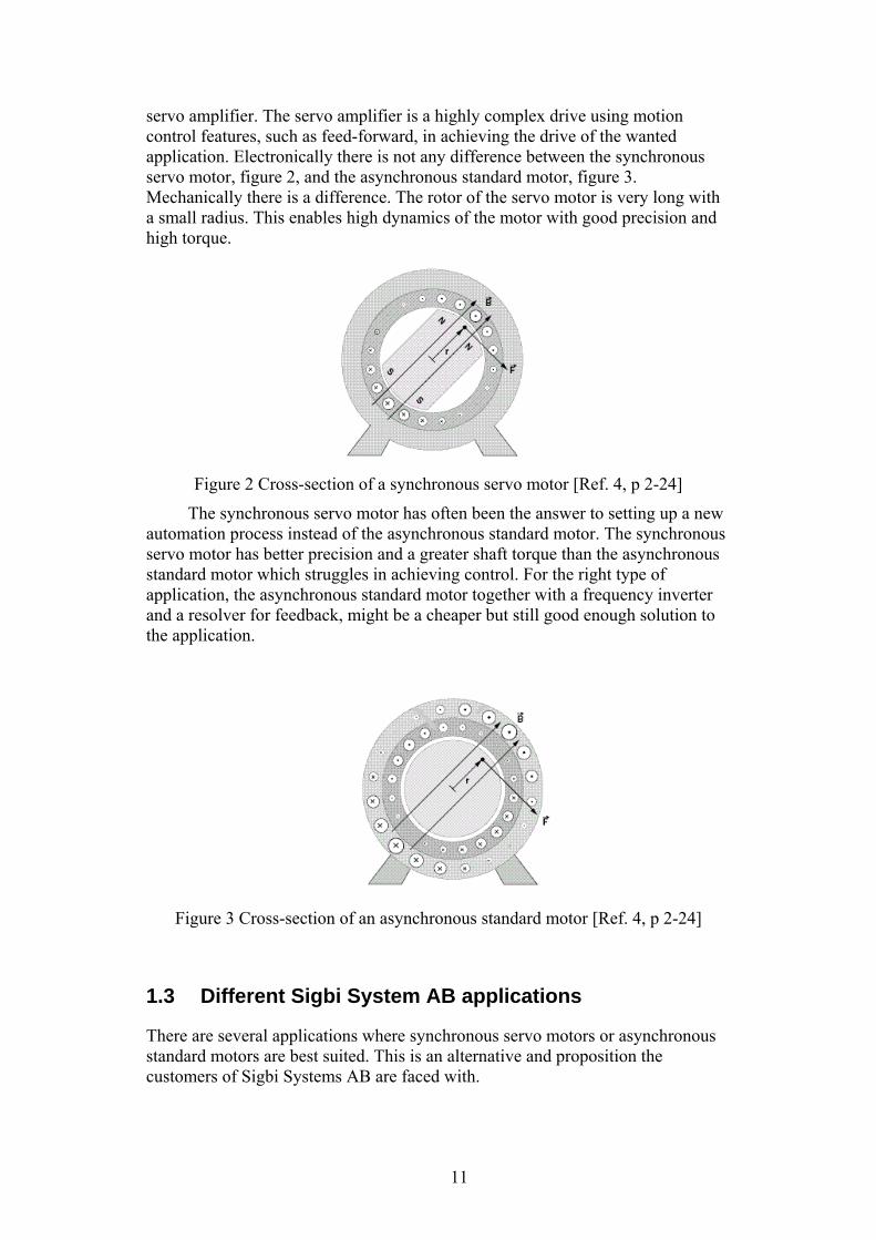
servo amplifier. The servo amplifier is a highly complex drive using motion control features, such as feed-forward, in achieving the drive of the wanted application. Electronically there is not any difference between the synchronous servo motor, figure 2, and the asynchronous standard motor, figure 3. Mechanically there is a difference. The rotor of the servo motor is very long with a small radius. This enables high dynamics of the motor with good precision and high torque.

Figure 2 Cross-section of a synchronous servo motor [Ref. 4, p 2-24]

The synchronous servo motor has often been the answer to setting up a new automation process instead of the asynchronous standard motor. The synchronous servo motor has better precision and a greater shaft torque than the asynchronous standard motor which struggles in achieving control. For the right type of application, the asynchronous standard motor together with a frequency inverter and a resolver for feedback, might be a cheaper but still good enough solution to the application.

Figure 3 Cross-section of an asynchronous standard motor [Ref. 4, p 2-24]

1.3 Different Sigbi System AB applications

There are several applications where synchronous servo motors or asynchronous standard motors are best suited. This is an alternative and proposition the customers of Sigbi Systems AB are faced with.

12

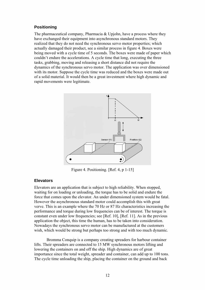
Positioning The pharmaceutical company, Pharmacia & Upjohn, have a process where they have exchanged their equipment into asynchronous standard motors. They realized that they do not need the synchronous servo motor properties; which actually damaged their product, see a similar process in figure 4. Boxes were being moved with a cycle time of 5 seconds. The boxes were made of paper which couldn’t endure the accelerations. A cycle time that long, executing the three tasks, grabbing, moving and releasing a short distance did not require the dynamics of the synchronous servo motor. The application was over dimensioned with its motor. Suppose the cycle time was reduced and the boxes were made out of a solid material. It would then be a great investment where high dynamic and rapid movements were legitimate.

Figure 4. Positioning. [Ref. 4, p 1-15]

Elevators Elevators are an application that is subject to high reliability. When stopped, waiting for on loading or unloading, the torque has to be solid and endure the force that comes upon the elevator. An under dimensioned system would be fatal. However the asynchronous standard motor could accomplish this with great verve. This is an example where the 70 Hz or 87 Hz characteristics increasing the performance and torque during low frequencies can be of interest. The torque is constant even under low frequencies; see [Ref. 10], [Ref. 11]. As in the previous application the object, this time the human, has to be taken into consideration. Nowadays the synchronous servo motor can be manufactured at the customers wish, which would be strong but perhaps too strong and with too much dynamic.

Bromma Conquip is a company creating spreaders for harbour container

lifts. Their spreaders are connected to 15 MW synchronous motors lifting and lowering the containers on and off the ship. High dynamics are of great importance since the total weight, spreader and container, can add up to 100 tons. The cycle time unloading the ship, placing the container on the ground and back

13

at the ship again, is only 60 seconds. Synchronous servo motors are beneficial in this type of demanding applications.

In figure 5, a direct-current (DC) diagram of a process in full speed into standstill is shown. It is picturing the current reference when precision and maintaining a certain shaft angle is required. This process was realized in the assembler coded program, see figure 10 and 11, and is also applicable in e.g. elevator designs. During brake the closed-loop direct-current is fed into the rotor, achieving a smooth stop through a force that counteract to the rotor torque, see [Ref. 12]. The bigger the slip, the stronger the dc current will be, minimizing the error.

Figure 5. Standstill torque. [Ref. 4, p 1-56]

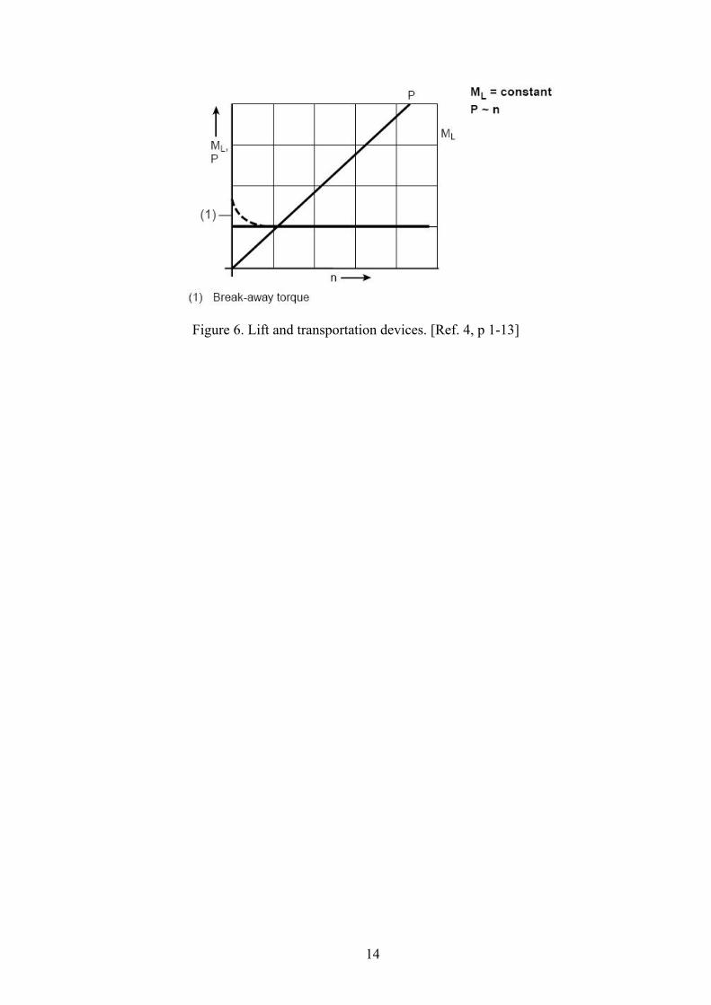
Both these two applications, the robot and the elevator, are characterized by

the standard load torque diagram in figure 6. When lifting an object the required torque is proportional to the vertical speed of the motor, as long as the load doesn’t change during start and stop that is.

14

Figure 6. Lift and transportation devices. [Ref. 4, p 1-13]

15

2. Problem Formulation

Sigbi Systems AB is interested in how the two AC-motors, the asynchronous standard motor and the synchronous servo motor, behave towards each other. Today there are advanced frequency inverters enabling advanced control of the asynchronous standard motors as a substitution to the reliable high dynamic synchronous servo motor. By choosing to install an asynchronous motor and a resolver or encoder together with a frequency inverter, you might save a great deal of money. So, will you loose performance by this setup compared to the high dynamic synchronous servo motor guarantees? How good are the two motors on step responses, sinus responses and also on following a predefined assembler coded program? The comparison of the two motors will be useful for evaluation of the boundaries between the applications where the inverter drive or the servo drive solution can be used.

16

3. Materials & Methods

3.1 Experimental platform

The experiments were performed at the laboratory at Sigbi Systems AB. A computer with the DriveManager software application from Sigbi Systems AB was used for the assignment. With this software, the frequency inverters can be setup for the appropriate control method. The frequency inverter being used for the assignment was manufactured at the company LUST, Germany. As feedback devices the asynchronous motor and the synchronous motor was fitted with a resolver. The frequency inverter helped not only with speed control but also with positioning control of the two motors.

3.2 Motor

Sigbi Systems AB supplied two different types of motors for the experiments. The first one, a water cooled synchronous motor called Bautz W406F and the second motor, a standard asynchronous ABB motor, 0.375 kW. Both motors had a power supply of 400 V.

3.3 Frequency inverters

The frequency inverter CDD3000, which also has the feature of a servo amplifier, was being used in the experiments. By switching between a frequency inverter for the asynchronous standard motor, and a servo amplifier for the synchronous servo motor, we minimize the addition of too many different components. This enables a strict comparison of the two motors.

With the use of the DriveManager software there are several setups to be

made. There is a tutorial to follow where the basic settings are being installed and where the parameters can be tuned to optimization.

The top speed was set at 1400 rpm on both motors. To get comparable

results on the motors, the servomotor was limited to a speed of 1400 rpm, disregarding its maximum speed of 6000 rpm.

To show the possible dynamics you can extract out of the two motors, the

acceleration was set at highest revolution/s2. Maximum acceleration was 1Hz/second, which resulted in an acceleration time of 50 ms.

3.4 Methods

The tests were made on the step and sinus responses. Data from both the reference values, as well as the actual values of speed and torque, was sampled. When

17

testing the sinus response, the frequency inverter was set to “speed control” in the DriveManager software. Speed control was also adapted when during the tests on step response. Testing the assembler code, the motors were to follow a pre-programmed drive where “positioning control” was loaded in the frequency inverter.

The experiments were all carried out using the black box model. The

different control model that was implemented in the frequency inverter by LUST was not known during the experiment supporting this paper.

Designing bode plots in the black box model I set the analogue audio oscillator at a specific frequency, logarithmic specified 1-100 Hz on the x-axis. The results at the different frequencies were calculated in the Matlab computer software. The frequencies that were being used over the x-axis were 1.0000 1.5849 2.5119 3.9811 6.3096 10.0000 15.8489 25.1189 39.8107 63.0957 100.0000

All plots that are presented in this paper, as well as all calculation and mathematical derivation, were extracted from scripts by the Matlab software. All scripts were made especially for this paper. To ease script calculation of the sampled data, Microsoft Excel was being used.

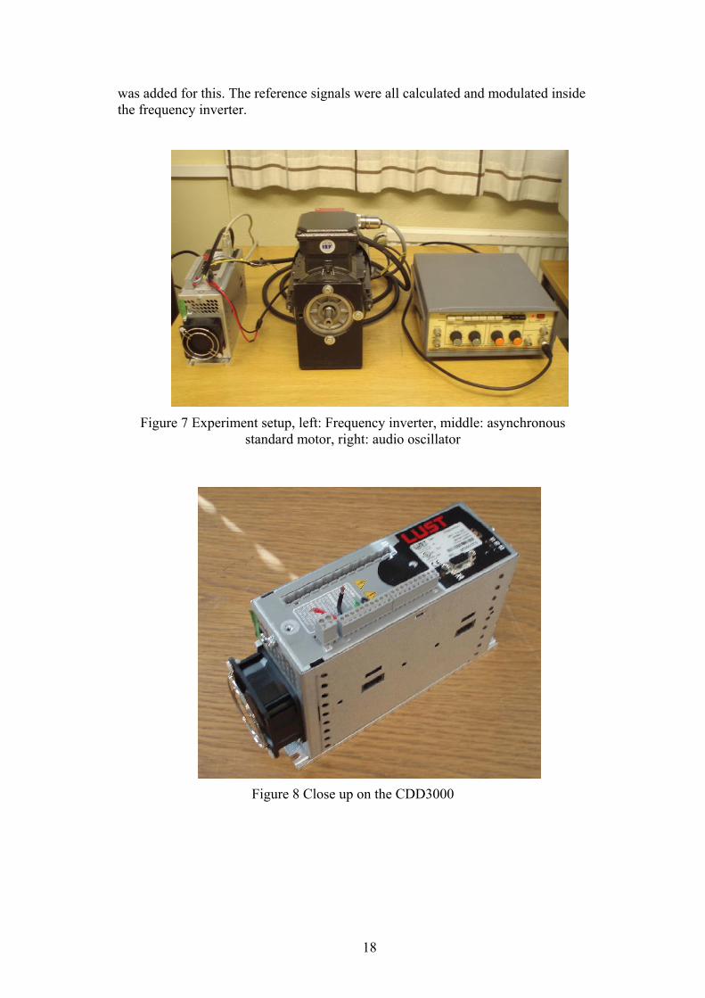
For the experiments regarding the sinus response, I used an audio oscillator to create a frequency reference signal for the frequency inverter to modulate, see figure 7.

With step response experiments, I used speed as reference. For the

assembler coded program positions were used as reference. No external hardware

18

was added for this. The reference signals were all calculated and modulated inside the frequency inverter.

Figure 7 Experiment setup, left: Frequency inverter, middle: asynchronous

standard motor, right: audio oscillator

Figure 8 Close up on the CDD3000

19

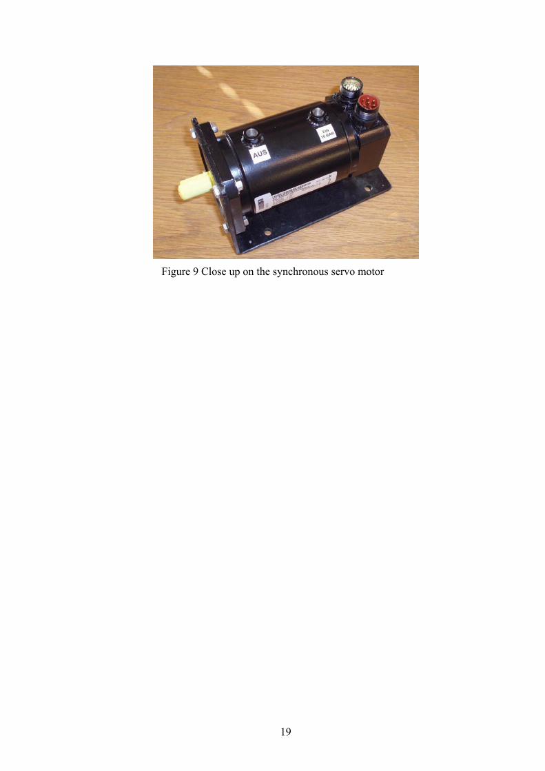
Figure 9 Close up on the synchronous servo motor

20

4. Interpolation programming

In processes in today’s factories, several motors often work together in interpolating patterns. Robots, for example, move in interpolating motions. This makes it possible to attack different soldering joints placed in different angels on a 3-D shaped object without moving the object into the right position.

In this section I programmed a motion drive of two motors interpolating

the shape of a circle. The choice of a circle as the shape was randomly chosen. I could have chosen a square or any other shape. A square would not be much of an interpolating challenge, since it all should be presented in a XY-coordinate system.

4.1 Hardware

Sigmatek is an Austrian company producing complete automation systems for machines and plant building. In this assignment I worked with an operating panel from Sigmatek called DTC281L. The demo controlled by the DTC281L was two frequency inverters from LUST, CDA3000, two asynchronous motors from ABB, two Kübler encoders with 2048 increments per revolution, and two linear units. The two motors had a maximum speed of 1400 rpm. The frequency inverters had a power supply of 230 V. DTC281L The DTC281L is an operating panel with a display and 28 buttons. Every button can be assigned with 100 different commands each. On the back and on the bottom, analog and digital outputs and inputs can be connected. On the bottom of the DTC281L I connected two analogue outputs to the frequency inverters for the reference signal. The reference signal is a +/- 10 Volt signal. All processing of the data is done with the DTC281L and its Intel 386EX processor. The Kübler encoders were also connected to the DTC281L.

21

Figure 10 DTC281L

Figure 11 The setup of the demo

4.2 Software

Two different kinds of software were used for programming the DTC281L. They were Lasal Class and Lasal Text.

22

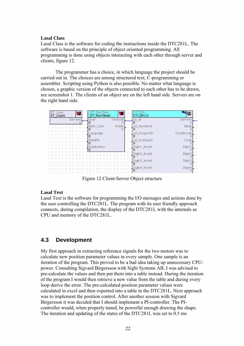
Lasal Class Lasal Class is the software for coding the instructions inside the DTC281L. The software is based on the principle of object oriented programming. All programming is done using objects interacting with each other through server and clients, figure 12.

The programmer has a choice, in which language the project should be

carried out in. The choices are among structured text, C-programming or assembler. Scripting using Python is also possible. No matter what language is chosen, a graphic version of the objects connected to each other has to be drawn, see screenshot 1. The clients of an object are on the left hand side. Servers are on the right hand side.

Figure 12 Client-Server Object structure

Lasal Text Lasal Text is the software for programming the I/O messages and actions done by the user controlling the DTC281L. The program with its user friendly approach connects, during compilation, the display of the DTC281L with the internals as CPU and memory of the DTC281L.

4.3 Development

My first approach in extracting reference signals for the two motors was to calculate new position parameter values in every sample. One sample is an iteration of the program. This proved to be a bad idea taking up unnecessary CPU-power. Consulting Sigvard Birgersson with Sigbi Systems AB, I was advised to pre-calculate the values and then put them into a table instead. During the iteration of the program I would then retrieve a new value from the table and during every loop derive the error. The pre-calculated position parameter values were calculated in excel and then exported into a table in the DTC281L. Next approach was to implement the position control. After another session with Sigvard Birgersson it was decided that I should implement a PI-controller. The PI-controller would, when properly tuned, be powerful enough drawing the shape. The iteration and updating of the states of the DTC281L was set to 0.5 ms

23

4.4 The shape

When creating the shape, a few things have to be determined in advance. In this case, when creating the shape of a circle, the diameter of the circle is important (CR, see table 1). The diameter of the circle can not be longer than the length of the braces (β1 and β2, see table 1 and figure 13) A brace in horizontal position is either located in cosine 0 or cosine 1 as well as the distance between the two units may not exceed the length of the braces. In this hardware setup it is the joint between the braces that makes the shape. In this assignment the braces are of equal length. The combination, the linear units and diameter of the circle, does also have restrictions, as we will se later. The number of parameters defining the shape is also declared in advance where, of course, the table start parameter is equal to the table end parameter. The more parameters in the table there are, the higher resolution the shape will have. Each motor has got a separate calculated table otherwise we would just get a straight vertical line; they are of equal length though. In the DTC281L the time of iteration is chosen before compilation. This makes the time completing the shape, dependent on the number of parameters, read in the position table which also is important assigning the number of rows in the table.

Theory of the position parameters The theory in finding the different parameters was done using trigonometry, sine, cosines and the Pythagorean Theorem. I defined the initiation point at cosines 1 and sine 0 moving the joint of the braces counterclockwise. The position parameter tables were defined by 4000 rows a.k.a. positions for the joint of the braces to follow.

4000 rows = a circle π2= (1)

α:th row/position/angle of circle πα 24000

×⎟⎠⎞

⎜⎝⎛= (2)

Calculations for the left motor (prefix 1, in figure 13) at α, see (1) and (2). Calculating katets inside the circle:

1. γ1 = γ2 = )(sin αeCR ∗ 2. PKu = )(cos αineCR ∗ 3. φ1 = HD + PKu

Step three has extracted the horizontal katet (φ1) from the left linear unit to the position the joint theoretically should be at. Now, two out of three variables in the Pythagorean Theorem are known. The only missing variable is the vertical katet (β1).

4. β1 = ( ) ( )21

21 ϕδ −

24

5. Final value for the left motor parameter at row α, LMp = β1 + γ1

Calculations for the right motor table (2, prefix in figure 13) at α

Calculating katets inside the circle: Step 1 and 2 from above are the same for the right motor calculations.

1. See above 2. See above 3. φ2 = HD - PKu

As for the left motor, step three calculates the horizontal katet (φ2) from the linear unit to the position the joint should be at.

4. β2 = ( ) ( )22

22 ϕδ −

5. Final value for the right motor parameter at row α, RMp = β2 + γ2

Figure 13 Theory for calculating parameters of a circle

25

Table of explanations and abbreviations used in calculations and from figure 13

• δ1 (Left Black hypotenuse) • δ2 (Right Black hypotenuse) • TG = BG (Top/Bottom green katet) • PKu (Purple katet inside unit circle) • LMp (Left Motor parameter) • RMp (Left Motor parameter) • CR (Circle radius) • HD (Distance between the linear units, divided in two)

Table 1

4.5 Problems, solutions and thoughts

During this project I had some serious voltage potentials with unshielded cables which later were removed. It was the frequency inverters, discussed in Section 1.2 of this paper, with their modulation that caused the disturbances. It resulted in really bad drives of the motors.

As the work progressed, and I was ready to test the program with the motors, I realized that the weight of the two linear units would be a problem. My first approach was to design a xy-coordinate system of the linear units. To horizontally attach one of the linear units on the vertical linear unit would be too heavy and unstable. It would also result in lack in precision since the load would differ a lot for the two motors. The linear units are quit heavy. At Sigbi Systems AB we tried to use a smaller linear unit but the height of a linear unit of 700 mm was not enough, the resolution became to low. After some discussion we decided to try and create the shape from the two vertical linear units as they were, vertically, standing up, figure 11. They would then be connected through two braces and the shape would be defined by the joint of the two braces as seen in figure 11 and figure 13.

When drawing the shape it is possible to either attach the braces to draw

the circle in an upwards motion or, as I did, in a downwards motion. The difference is just a theoretically recalculation of the position parameters. The distance between the two linear units is not a problem, since the length of the braces determines the diameter as long as the braces can be fitted together. One has to be aware of the length of the braces and the material they are made of. If the braces aren’t strong enough and the speed of the motion is high, poor ocular accuracy will be the result.

The length of the linear units has to be longer than the diameter of the

circle (δ1 and δ2, figure 13). Example: (see figure 14, not a scaled figure) The direction is counterclockwise starting at degree 0. Towards 0.5π both

braces are going upwards. At position 1, see figure 14, the right motor has its peak value. This position is defined as the position where δ2, figure 13, becomes the

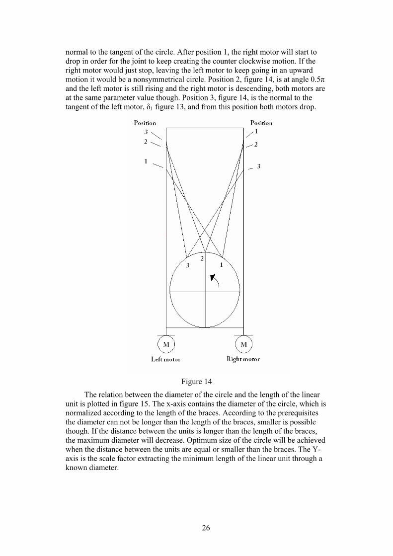
26

normal to the tangent of the circle. After position 1, the right motor will start to drop in order for the joint to keep creating the counter clockwise motion. If the right motor would just stop, leaving the left motor to keep going in an upward motion it would be a nonsymmetrical circle. Position 2, figure 14, is at angle 0.5π and the left motor is still rising and the right motor is descending, both motors are at the same parameter value though. Position 3, figure 14, is the normal to the tangent of the left motor, δ1 figure 13, and from this position both motors drop.

Figure 14

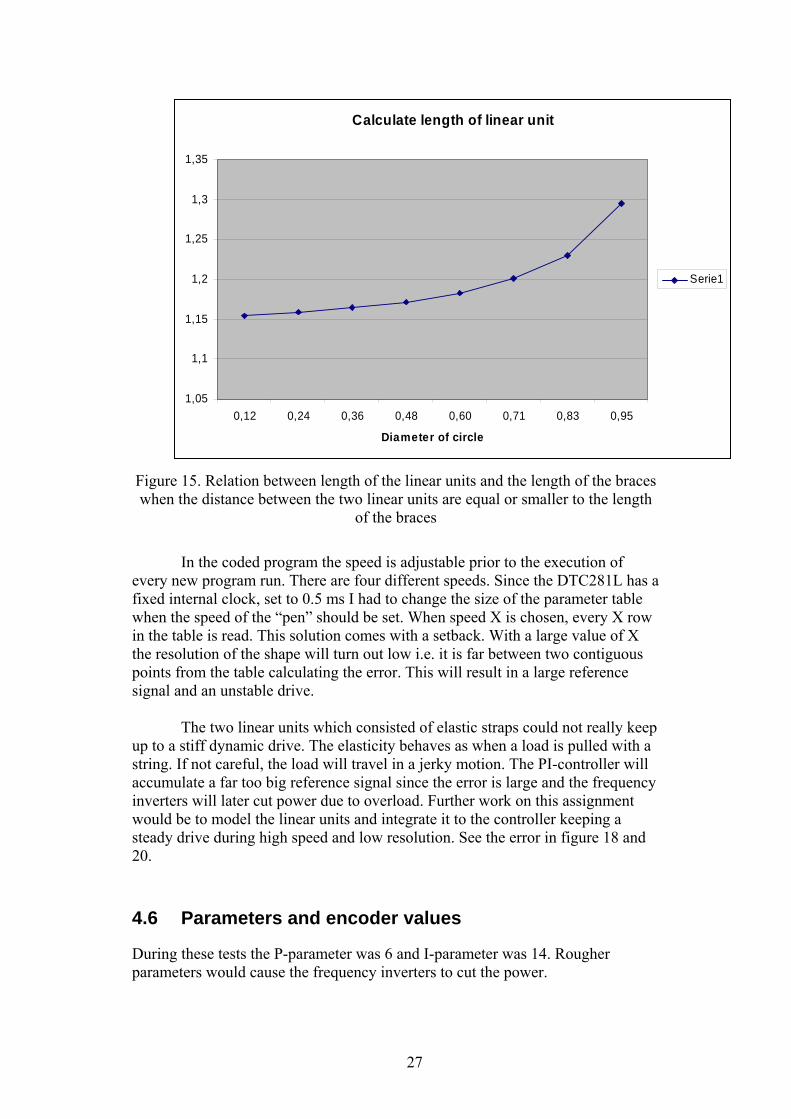
The relation between the diameter of the circle and the length of the linear unit is plotted in figure 15. The x-axis contains the diameter of the circle, which is normalized according to the length of the braces. According to the prerequisites the diameter can not be longer than the length of the braces, smaller is possible though. If the distance between the units is longer than the length of the braces, the maximum diameter will decrease. Optimum size of the circle will be achieved when the distance between the units are equal or smaller than the braces. The Y-axis is the scale factor extracting the minimum length of the linear unit through a known diameter.

27

Calculate length of linear unit

1,05

1,1

1,15

1,2

1,25

1,3

1,35

0,12 0,24 0,36 0,48 0,60 0,71 0,83 0,95

Diameter of circle

Serie1

Figure 15. Relation between length of the linear units and the length of the braces when the distance between the two linear units are equal or smaller to the length

of the braces

In the coded program the speed is adjustable prior to the execution of

every new program run. There are four different speeds. Since the DTC281L has a fixed internal clock, set to 0.5 ms I had to change the size of the parameter table when the speed of the “pen” should be set. When speed X is chosen, every X row in the table is read. This solution comes with a setback. With a large value of X the resolution of the shape will turn out low i.e. it is far between two contiguous points from the table calculating the error. This will result in a large reference signal and an unstable drive.

The two linear units which consisted of elastic straps could not really keep

up to a stiff dynamic drive. The elasticity behaves as when a load is pulled with a string. If not careful, the load will travel in a jerky motion. The PI-controller will accumulate a far too big reference signal since the error is large and the frequency inverters will later cut power due to overload. Further work on this assignment would be to model the linear units and integrate it to the controller keeping a steady drive during high speed and low resolution. See the error in figure 18 and 20.

4.6 Parameters and encoder values

During these tests the P-parameter was 6 and I-parameter was 14. Rougher parameters would cause the frequency inverters to cut the power.

28

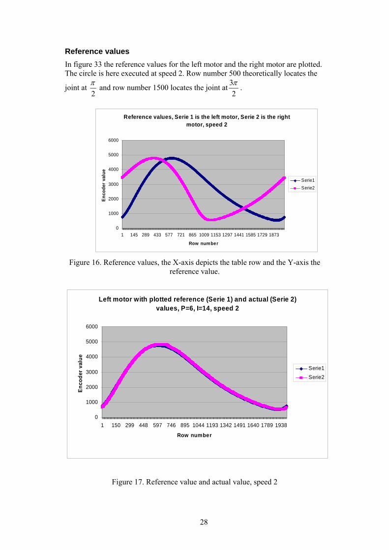
Reference values In figure 33 the reference values for the left motor and the right motor are plotted. The circle is here executed at speed 2. Row number 500 theoretically locates the

joint at 2π and row number 1500 locates the joint at

23π .

Reference values, Serie 1 is the left motor, Serie 2 is the right motor, speed 2

0

1000

2000

3000

4000

5000

6000

1 145 289 433 577 721 865 1009 1153 1297 1441 1585 1729 1873

Row number

Enco

der

valu

e

Serie1Serie2

Figure 16. Reference values, the X-axis depicts the table row and the Y-axis the

reference value.

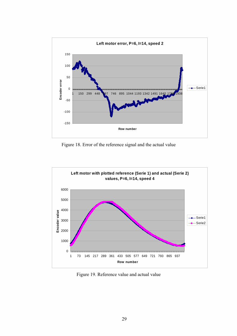
Left motor with plotted reference (Serie 1) and actual (Serie 2) values, P=6, I=14, speed 2

0

1000

2000

3000

4000

5000

6000

1 150 299 448 597 746 895 1044 1193 1342 1491 1640 1789 1938

Row number

Enco

der v

alue

Serie1Serie2

Figure 17. Reference value and actual value, speed 2

29

Left motor error, P=6, I=14, speed 2

-150

-100

-50

0

50

100

150

1 150 299 448 597 746 895 1044 1193 1342 1491 1640 1789 1938

Row number

Enco

der e

rror

Serie1

Figure 18. Error of the reference signal and the actual value

Left motor with plotted reference (Serie 1) and actual (Serie 2) values, P=6, I=14, speed 4

0

1000

2000

3000

4000

5000

6000

1 73 145 217 289 361 433 505 577 649 721 793 865 937

Row number

Enco

der v

alue

Serie1Serie2

Figure 19. Reference value and actual value

30

Left motor error, P=6, I=14, speed 4

-200

-150

-100

-50

0

50

100

150

200

250

300

1 73 145 217 289 361 433 505 577 649 721 793 865 937

Row number

Enco

der e

rror

Serie1

Figure 20. Error of the reference signal and the actual value

.

Comparing figure 17 and 19 there is hardly any difference between the reference signal and the actual signal, not to the naked eye anyway. Looking at figure 18 and 20 the error is more noticeable. The error per table row is almost two times higher at speed 4 than speed 2, figure 20 and figure 18. At speed 4 the error peaks at about 250 increments i.e. 12% of a revolution. The error at the left motor is at its highest reaching for position 1; see figure 14. The error becomes negative after row number 500 and 250 which is the top position of the circle at speed 2 and speed 4, figure 18 and figure 20.

4.7 Different proportional gain and integral part

Different tests were made changing the proportional gain and the integral part in the program. All tests were made at the highest speed, speed number 4.

31

Left motor error, P=3, I=8, Speed=4

-400

-300

-200

-100

0

100

200

300

400

500

600

1 73 145 217 289 361 433 505 577 649 721 793 865 937

Row number

Enco

der e

rror

Serie1

Figure 21 Error of the reference signal and the actual value

Left motor error, P=3, I=14, Speed=4

-600

-400

-200

0

200

400

600

800

1 73 145 217 289 361 433 505 577 649 721 793 865 937

Row number

Enco

der

erro

r

Serie1

Figure 22 Error of the reference signal and the actual value

32

Left motor error, P=6, I=8, Speed=4

-200

-150

-100

-50

0

50

100

150

200

250

300

1 73 145 217 289 361 433 505 577 649 721 793 865 937

Row number

Enco

der e

rror

Serie1

Figure 23 Error of the reference signal and the actual value

Left motor error, P=6, I=14, speed 4

-200

-150

-100

-50

0

50

100

150

200

250

300

1 73 145 217 289 361 433 505 577 649 721 793 865 937

Row number

Enco

der

erro

r

Serie1

Figure 24 Error of the reference signal and the actual value

33

Left motor error, P=9, I=8, Speed=4

-150

-100

-50

0

50

100

150

200

1 73 145 217 289 361 433 505 577 649 721 793 865 937

Row number

Enco

der e

rror

Serie1

Figure 25 Error of the reference signal and the actual value

Left motor error, P=9, I=14, Speed=4

-150

-100

-50

0

50

100

150

200

250

1 73 145 217 289 361 433 505 577 649 721 793 865 937

Row number

Enco

der

erro

r

Serie1

Figure 26 Error of the reference signal and the actual value

From the figures 21 to 26 the proportional gain is set to 3, 6 and 9 combined with an integral part of 8 and 14. Testing the programs with the different parameters the setup, P=6 and I=14, was the smoothest drive. Mathematically the last setting in figure 26, P=9 and I=14, proved too have the smallest error, table 2.

34

Parameters P=3, I=8 P=3, I=14 P=6, I=8 P=6, I=14 P=9, I=8 P=9, I=14 Encoder error (inc) 215 191 118 102 91 76

Table 2, average error increments per table row Due to the elastic straps the visible result tends to be jerkier the higher the proportional gain I use, even though the error in table 5 decreases. Increasing the proportional gain even more at speed 4, will accumulate an overload at the frequency inverter.

4.8 Flowchart

Figure 27. Flowchart of the program compiled inside the DTC281L

4.9 Manual

1. Run a program. Start one out of several different programs. 2. Stop the program. During a program-run there is a stop-button

on the panel for immediate stop. 3. Set the speed of the “Pen.” The process can be set at different

speed modes.

35

Run a program

1.1 Press the upper left button saying “Program”. 1.2 Press any of the “P[ ]” buttons. 1.3 The homing is initiated. 1.4 Press the left button, “Start”, to run the program.

Stop the program 2.1 Press the right button saying “Stop”. 2.2 Either press “Resume” resuming the process or press “Back” to

return to the initial view and the start position is initiated once more. Set the speed of the joint/“Pen”

3.1 From the root, press the upper right button saying “Settings” 3.2 By the arrow buttons left and right the speed can be set.

36

5. Results

5.1 Assembler coded program

Figure 28. Torque plot

Figure 29. Torque plot

37

In figure 28 the assembler coded program is executed on the asynchronous

standard motor. In figure 29 the data from the synchronous servo motor is plotted. The motors follow their torque reference signal quite nicely but there is a great difference in magnitude.

5.2 Bode diagram

Figure 30

Figure 31

38

The asynchronous standard motor, figure 30 and figure 31, shows it’s dynamics with and without load, at low and high frequencies. Above 10 Hz it works as a high pass filter. The phase margin never passes below -50 degrees or above 100 degrees.

Figure 32

Figure 33

The asynchronous standard motor, figure 32 and figure 33, is run with speed as the reference signal. The high pass filter is not as apparent as when torque was the reference signal, although the phase margin is almost the same. Without load it

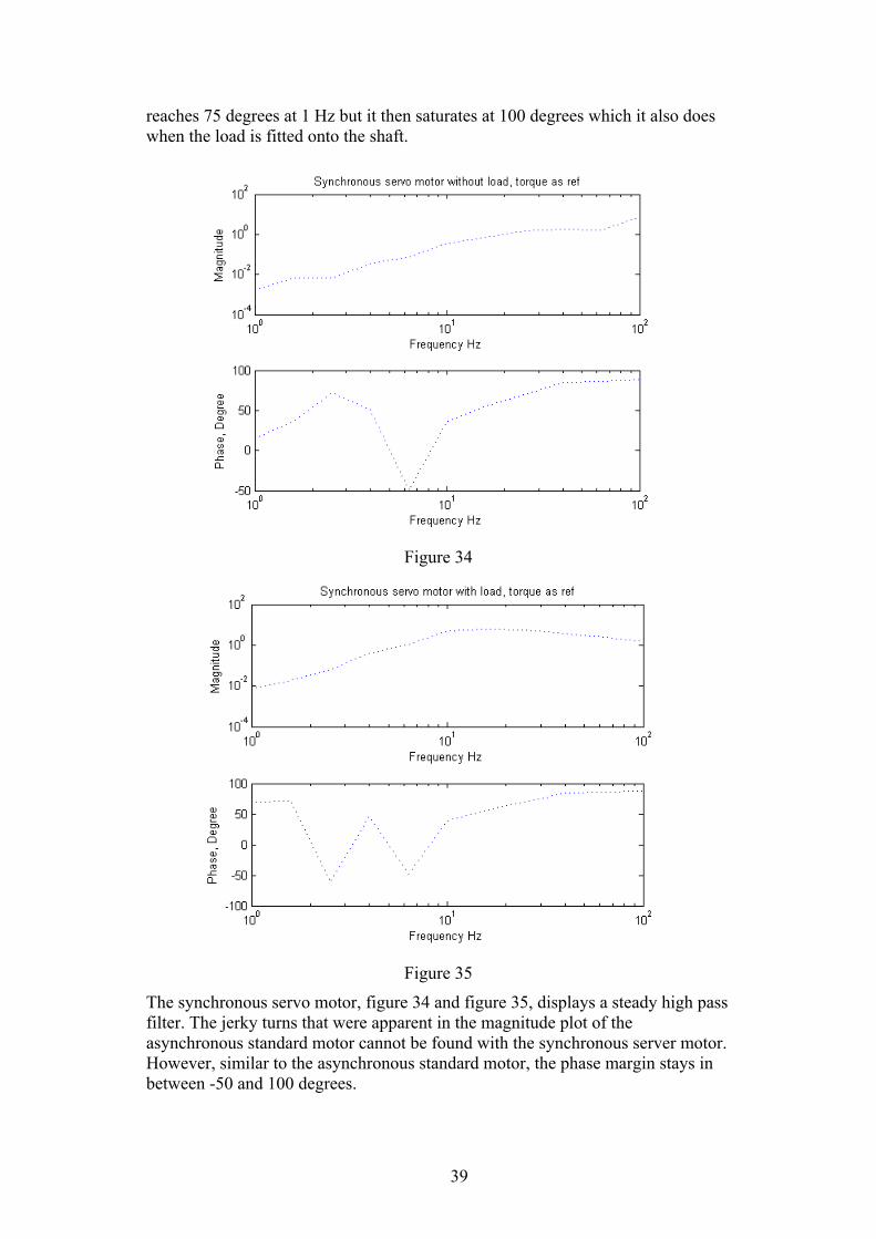
39

reaches 75 degrees at 1 Hz but it then saturates at 100 degrees which it also does when the load is fitted onto the shaft.

Figure 34

Figure 35

The synchronous servo motor, figure 34 and figure 35, displays a steady high pass filter. The jerky turns that were apparent in the magnitude plot of the asynchronous standard motor cannot be found with the synchronous server motor. However, similar to the asynchronous standard motor, the phase margin stays in between -50 and 100 degrees.

40

Figure 36

Figure 37

With load fitted to the shaft and speed as reference signal, figure 36 and figure 37, there is a significant difference compared to running the motor without any load. At high frequencies and a fitted load the magnitude returns to the same low value as for low frequencies. The phase margin is in this last experiment is between -75 and 100 degrees.

41

5.3 Step response

Figure 38

Figure 39

42

The step responses, figure 38 and figure 39, have been recorded as the parameters were plugged into the frequency inverter. In figure 38 the asynchronous standard motor is plotted. In figure 39 the synchronous servo motor is plotted. The overshoot is at about 20 % above the expected value for both motors. The average error per sample from the step responses: Speed Error (rpm/sample) 100rpm 500rpm 1000rpm 1300rpmAsynchronous standard motor 0.1614 0.6358 1.4956 1.9099 Synchronous servo motor 0.7664 2.7201 7.2888 9.3624

Table 3

Torque Error (Nm/sample) 100rpm 500rpm 1000rpm 1300rpmAsynchronous standard motor 0.0253 0.0290 0.0670 0.0906 Synchronous servo motor 0.0042 0.0045 0.0052 0.0055

Table 4

43

6. Discussion

The initial tuning of the frequency inverter CDD3000 was to set the overshoot of the two motors to 20 %. The CDD3000 is loaded with the motor data parameters which help the frequency inverter to optimize the control for each individual motor due to their mechanical construction. Both motors were tuned with the initial speed of 100 rpm resulting in a reference signal and an overshoot of a total of 120 rpm. The tuning of the frequency inverter parameters is a very complex task though as can be seen in the step response, figure 38 and figure 39.

6.1 Assembler program

Figure 40, Torque control time [Ref. 4, p 1-11]

In the assembler program plot, figure 29, it is shown that during the first sample of the synchronous servo motor, a torque of 4.34 Nm is needed which actually is developed inside the synchronous servo motor, see red and blue curve. The actual value is on a small overshoot at the time 8.5ms, according to the data files, which states the torque control time to be less than 8.5ms. With figure 40 in mind, looking at the asynchronous standard motor, figure 28, 95% of the wanted torque is reached in approximately 25ms. This results in a torque control time of about 25ms.

Theoretically, it’s known, that the slow internal time constant is the drawback of the asynchronous standard motor. When examining the torque from the two different motors, see figure 28 and figure 29, the advantage of using a synchronous servo motor, instead of an asynchronous standard motor, is obvious. The time constant of the synchronous servo motor also enables the frequency inverter to modulate a more aggressive reference signal developing high

44

dynamics. This results in a torque magnitude of about four times the asynchronous standard motor when the motors are exposed to turns affecting the motor in opposite direction. The powerful qualities possessed by the synchronous servo motor which should be considered when customizing and developing the application is hereby shown.

Depending on the mechanical setup of the asynchronous standard motor and the synchronous servo motor, the accuracy of torque control differ between the two motors. The accuracy of the asynchronous standard motor is dependent on several machine parameters, i.e. temperature dependent parameters. The stationary relative accuracy is approximately ±10%. As for the synchronous servo motors concerned, the stationary relative accuracy is ±2%. [Ref. 4, p 2-19]

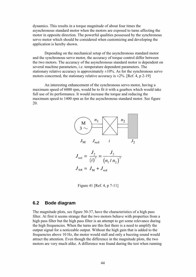
An interesting enhancement of the synchronous servo motor, having a maximum speed of 6000 rpm, would be to fit it with a gearbox which would take full use of its performance. It would increase the torque and reducing the maximum speed to 1400 rpm as for the asynchronous standard motor. See figure 20.

Figure 41 [Ref. 4, p 7-11]

6.2 Bode diagram

The magnitude plots, see figure 30-37, have the characteristics of a high pass filter. At first it seems strange that the two motors behave with properties from a high pass filter but the high pass filter is an attempt to get some relevance during the high frequencies. When the turns are this fast there is a need to amplify the output signal for a noticeable output. Without the high gain that is added to the frequencies above 10 Hz, the motor would stall and only a buzzing sound would attract the attention. Even though the difference in the magnitude plots, the two motors are very much alike. A difference was found during the test when running

45

on higher frequencies. The synchronous servo motor, with its fast time constant, resulted in a far greater visible response.

The resulting smoothness in the magnitude plots of the synchronous servo

motor, figure 34-37, compared to the asynchronous standard motor, figure 30-33, is due to the high dynamics of the synchronous servo motor. A small error between the reference signal and the actual value results in a reduction of the angularity in the interpolation of the plots. This is shown in the synchronous servo motor bode plots, figure 30-33. A smooth curve shows high dynamics and high dynamics lead to good control when the process is adapting to the reference signal, minimizing the error. The result is a reliable drive.

For the phase margin concerned there are, unfortunately, not enough sample

points in the data files to interpolate the phase margin for low frequencies. From the plots, the jerky interpolation can’t, in an accurate way, describe what happens below 10 Hz. Since there is a high demand on these motors, they have been sold out at Sigbi Systems AB and the experiments can’t be redone. This, unfortunately, leaves me to only comment on the interpolation above 10 Hz. Common to all the phase margin plots, see figure 30-37, they all saturate at 90 degrees for high frequencies, no matter a synchronous servo motor or an asynchronous standard motor. Nor does it matter fitted to a load or not. The phase margin plot shows great stability at high frequencies where the transfer function never enfolds –π, the Nyquist Theorem. The process might result in a slow control due to a great stability margin, [Ref. 6, p 51], affecting the asynchronous standard motor the most because of its slow time constant.

6.3 Step response

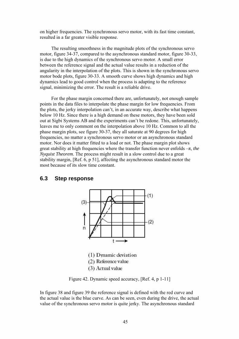
Figure 42. Dynamic speed accuracy, [Ref. 4, p 1-11]

In figure 38 and figure 39 the reference signal is defined with the red curve and the actual value is the blue curve. As can be seen, even during the drive, the actual value of the synchronous servo motor is quite jerky. The asynchronous standard

46

motor though, proves to have a much more controlled drive closer to the reference signal and much smaller dynamical speed accuracy, see figure 42. This is once more a consequence from the tuning not being 100% optimized for the synchronous servo motor.

Figure 39 actually contradicts the behaviour of the synchronous servo

motor compared to the asynchronous standard motor, figure 38. Later on in this section we will see the advantage the synchronous servo motor possesses in terms of high dynamic even though, at this point, it appears that it will not fulfil the step response tasks as well as the asynchronous standard motor does.

6.4 Average error

The test on the average error is made on the sampled data from different step responses with different speed. The error seen in Table 3 considers the speed error and Table 4 illustrates the error considering the torque. During constant speed the asynchronous standard motor have a lower speed error of about 4-5 times compared to the synchronous servo motor, see table 3. In table 4 the torque error is about 5-6 times smaller by the synchronous motor at lower speeds. Reaching a top speed at 1300 rpm the synchronous motor has an error of about 16 times lower than the asynchronous motor per sample.

This test really shows the unnecessary use of a synchronous servo motor in a poor analyzed environment when driving a motor in one direction without any change in the load. The error per sample is, in this experiment, far smaller for the asynchronous standard motor, which might be a very reasonable and acceptable error for the application. It is all about fitting appropriate equipment for the required demands. Over dimensioning is ineffective and cost money.

6.5 Overheat

Due to the permanent magnet, fitted inside the rotor of the synchronous servo motor, no magnetization is required, [Ref. 13, p 12]. This reduces its energy loss by 50%, improving its efficiency. If the motor is suitable for the application, it will not overheat, it is confirmed by the nominal torque (Mn) and the effective torque (Meff). See figure 43.

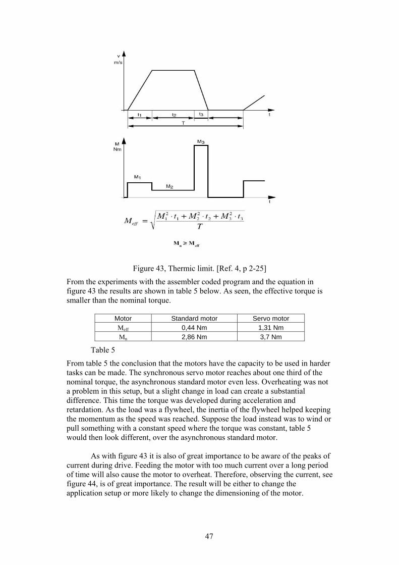
47

Figure 43, Thermic limit. [Ref. 4, p 2-25]

From the experiments with the assembler coded program and the equation in figure 43 the results are shown in table 5 below. As seen, the effective torque is smaller than the nominal torque.

Motor Standard motor Servo motor Meff 0,44 Nm 1,31 Nm Mn 2,86 Nm 3,7 Nm

Table 5

From table 5 the conclusion that the motors have the capacity to be used in harder tasks can be made. The synchronous servo motor reaches about one third of the nominal torque, the asynchronous standard motor even less. Overheating was not a problem in this setup, but a slight change in load can create a substantial difference. This time the torque was developed during acceleration and retardation. As the load was a flywheel, the inertia of the flywheel helped keeping the momentum as the speed was reached. Suppose the load instead was to wind or pull something with a constant speed where the torque was constant, table 5 would then look different, over the asynchronous standard motor.

As with figure 43 it is also of great importance to be aware of the peaks of current during drive. Feeding the motor with too much current over a long period of time will also cause the motor to overheat. Therefore, observing the current, see figure 44, is of great importance. The result will be either to change the application setup or more likely to change the dimensioning of the motor.

48

Figure 44. Machine load. [Ref. 4, p 1-52]

49

7. Conclusion

In the matter of high reliability and heavy loads that need high precision in speed and position, the synchronous servo motor is outstanding. The design of the synchronous motor, with the long radial axle and a smaller diameter, promotes a shorter and faster time constant and is for sure the winning concept. In the end it all comes down to the customer’s needs. It is not so much loosing performance in choosing an asynchronous standard motor, instead of the synchronous servo motor, as it is doing a fair analysis and installing a motor capable of the required needs. Both motors can work as components in lifts or positioning applications.

Running an application, where constant speed is needed, an asynchronous

motor connected to a frequency inverter should of course be reconsidered. If the application has a high load but can tolerate an acceleration time to nominal speed >100ms, then the asynchronous standard motor is a great substitute to a synchronous drive system. When the process demands quicker turns, then the asynchronous standard motor can’t keep up to the reference signal. If the acceleration has an upper limit of 50ms it is inevitable to install a synchronous servo motor. In between 50ms and 100ms some careful calculations has to be made whether what drive to use.

In a robot driven sorting system, where the product is solid and the

positioning of the product is of great importance, the synchronous servo motor is to be preferred. If the positioning drive system should handle fragile objects a synchronous servo motor might cause damage to the product. E.g. in a lift application, say an elevator, an asynchronous standard motor, a pure energy inverter, should definitely be installed. It is not reasonable to reach nominal speed within 100ms. With the synchronous servo motor, an optimized impulse inverter, its pros in performance and dynamics would not be extracted to its fullest in a realistic elevator drive system.

The price of the synchronous servo motor and servo drive is high but you

gain extreme performance. Due to the price of the drive system, the demands can be reduced by setting up an asynchronous standard motor instead. An advantage the synchronous motor has is the size of the motor. It is smaller than the asynchronous standard motor; with a narrow space this would come handy. All asynchronous standard motors are, standard, thereof the name, so changing between different manufactures is not a problem. The asynchronous standard motors and the frequency inverters are also components in stock. Buying a spare part is quick and easy.

Serious analysis can save a great deal of energy, money and efficiency, or tune the already existing drive system.

50

8. References

1: W. Leonard, Control of Electrical Drives, Springer, Institut für Regelungstechnik Hans Sommer Strasse 66 D-38106 Braunschweig, 1997 2: Danfoss A/S, Värt att veta om frekvensomriktare, Chr.Hendriksen & Søn, Skive, 1998 3: Åke Sjödin, Frekvensomriktare, Elforsk, Olof Palmes Gata 31 101 53 Stockholm, 2004 4: SIGBI System AB, Drivteknik och automatisering, Pinnmogatan 1 254 64 Helsingborg, 2000 5: Karl-Erik Årzén, Real-Time Control Systems, Department of Automatic Control Lund Institute of Technology, 2003 6: Tore Hägglund, Reglerteknik AK, Institutionen för reglerteknik Lunds Tekniska Högskola, Maj 2003 7: Rolf Johansson, System Modeling & Identification, Prentice Hall, PO Box 118 S-221 00 Lund, 2004 8: http://ecmweb.com/ops/electric_direct_current_motor/ 9: http://www.tpub.com/content/neets/14177/ 10: http://www.sigbi.se/elmotordrifter/70hz_karakteristik.htm 11: http://www.sigbi.se/elmotordrifter/87hz_karakteristik.htm 12: http://www.sigbi.se/Diverse/Downloads/kap_1.pdf , see chapter 1.13.8 13: http://www.kfb.se/pdfer/R-00-57.pdf