inverse retinotopy: inferring the visual content of images from brain activation patterns

www.elsevier.com/locate/ynimg
NeuroImage 33 (2006) 1104–1116
Inverse retinotopy: Inferring the visual content of images from brainactivation patterns

Bertrand Thirion,a,⁎ Edouard Duchesnay,b Edward Hubbard,d Jessica Dubois,c

Jean-Baptiste Poline,c Denis Lebihan,c and Stanislas Dehaened

aINRIA Futurs, Service Hospitalier Frédéric Joliot, 4, Place du Général Leclerc 91401 Orsay Cedex, FrancebUnité INSERM ERM 0205, Service Hospitalier Frédéric Joliot, 4, Place du Général Leclerc, 91401 Orsay Cedex, FrancecCEA, DSV, DRM, SHFJ 4, Place du Général Leclerc, 91401 Orsay Cedex, FrancedUnité INSERM 562 “Neuroimagerie Cognitive” Service Hospitalier Frédéric Joliot, 4 Place du Général Leclerc, 91401 Orsay Cedex, France

Received 12 January 2006; revised 26 June 2006; accepted 28 June 2006Available online 9 October 2006

Traditional inference in neuroimaging consists in describing brainactivations elicited and modulated by different kinds of stimuli.Recently, however, paradigms have been studied in which the converseoperation is performed, thus inferring behavioral or mental statesassociated with activation images. Here, we use the well-knownretinotopy of the visual cortex to infer the visual content of real orimaginary scenes from the brain activation patterns that they elicit. Wepresent two decoding algorithms: an explicit technique, based on thecurrent knowledge of the retinotopic structure of the visual areas, andan implicit technique, based on supervised classifiers. Both algorithmspredicted the stimulus identity with significant accuracy. Furthermore,we extend this principle to mental imagery data: in five data sets, ouralgorithms could reconstruct and predict with significant accuracy apattern imagined by the subjects.© 2006 Elsevier Inc. All rights reserved.

Introduction

The neuroimaging inverse problem

Validation of anatomo-functional knowledge produced fromneuroimaging data is a difficult task. While statistical significance,reproducibility and multi-modal coherence are well-acceptedproofs of consistency, neuroscientists lack a gold standard toassess the significance of their findings. A possible way to solvethis issue is to reason as follows: understanding a cognitivesubsystem of the brain means that the stimulus-to-activation chainhas been identified. More precisely, although the detailedmechanisms of neural and hemodynamic activation are not fullyunderstood, we can expect that a controlled stimulus (e.g. aflashing checkerboard) will produce a known pattern of activation.

⁎ Corresponding author.E-mail address: [email protected] (B. Thirion).Available online on ScienceDirect (www.sciencedirect.com).

1053-8119/$ - see front matter © 2006 Elsevier Inc. All rights reserved.doi:10.1016/j.neuroimage.2006.06.062

When this holds, the processing chain can be inverted, leading toactivation-to-stimulus inference. When possible, this inverseinference allows good performance characterization, since theresults are expressed in terms of predicted versus true stimulus, inthe well-known (and controlled) stimulus space.

This point of view has already been investigated in the case ofmotor experiments (Dehaene et al., 1998), mental imagery(O'Craven and Kanwisher, 2000), counting/subitizing (Piazza etal., 2003), the notion of object categories (Haxby et al., 2001;Carlson et al., 2003; Cox and Savoy, 2003), the orientation of visualstimuli (Haynes and Rees, 2005; Kamitani and Tong, 2005) and liedetection (Davatzikos et al., 2005). It has been popularized under theconcept of brain reading. This novel approach in neuroimaging hasbeen facilitated by the use of data classification techniques such asLinear Discriminant Analysis (LDA) (Carlson et al., 2003) and morerecently, Support Vector Machines (SVM) (Cox and Savoy, 2003;LaConte et al., 2005) that can take functional images as input andclassify them into categories (supervised classification). But in thatcase the activation-to-stimulus function remains implicit, i.e. it isembedded in a set of learning samples, each one being associatedwith a known stimulus. An important question is whether thisbinding may be made explicit.

There is at least one system in which the stimulus-to-activationcoding is known explicitly: this is the case of retinotopy, where thespatial layout of an image is in the visual field also spatially encoded inthe primary visual cortex (Sereno et al., 1995). The inverse problemconsists in predicting the spatial layout of an activation pattern(stimulus) given a functional activation image. We address thisproblem with two kinds of analysis tools: supervised classification(based on SVMs) and an explicit inversion of the stimulus-to-activation function (inverse retinotopy). In this paper, we study twodifferent situations: a visual stimulation experiment, in which thesubject passively views a sequence of stimuli chosen among a discreteset and a mental imagery experiment in which the subject is asked toimagine a self-selected pattern chosen among the presented stimuli.

mailto:[email protected]

http://dx.doi.org/10.1016/j.neuroimage.2006.06.062

1105B. Thirion et al. / NeuroImage 33 (2006) 1104–1116

Retinotopy of the human visual cortex

It is well known that the human visual cortex is retinotopicallyorganized, at least in early areas. Retinotopic mapping, based on atravelling wave paradigm, is a standard procedure in the fMRIliterature (see e.g. Sereno et al., 1995; DeYoe et al., 1996; Tootellet al., 1996, 2003; Engel et al., 1997; Warnking et al., 2002;Dougherty et al., 2003; Wotawa et al., 2005). It is frequentlyperformed in order to delineate the early visual areas (V1, V2, V3,V3a, VP), which can be characterized by a visual field sign (VFS)(Sereno et al., 1995). By contrast, we interpret here the retinotopicinformation as a forward mapping from the visual field to thevisual cortex: we assume that there exists a transfer function thatmaps visual stimulation patterns to the primary visual cortex. Inthis work, the retinotopic data are used to estimate the transferfunction. This kind of model has been suggested for V1 (Tootell etal., 1998b), and is supported by recent experiments (Hansen et al.,2004). In our setting, we take into account the receptive fieldstructure (Smith et al., 2001) that characterizes the responsivity ofcortical neurons to retinal stimulation. Let us note, however, thatsuch a model ignores some parts of the response (non-linear and/ornegative components) (Shmuel et al., 2002, 2006).

In a recent paper (Vanni et al., 2005), a direct estimation of thetransfer function has been proposed based on randomized visualstimulation in an event-related design. However, this procedure isnot as generic as the phase-encoded retinotopic experiments and itcan only delineate predefined regions of the visual field.

Inverse reconstruction and classification

Assume that we are given a set of brain activation images ϕ1,…, ϕn associated with a set of stimuli σ1,…, σn chosen within afinite set S. Supervised classification and inverse reconstructionperform two kinds of characterization on these data:

• In the inverse reconstruction framework, we assume that aforward operator T that models the stimulus-to-activationprocess has been defined. The inverse reconstruction consistsin estimating the stimulus pattern ρi=T−1ϕi, i=1…n in order toidentify the label σi, i=1…n of the reconstructed pattern. Theperformance of the procedure can thus also be expressed interms of correct prediction rate. While this procedure requiresthe prior knowledge of the operator T, it applies to any activationimage, and understanding the failures of the system might beeasier, since the intermediate results ρi, i=1…n are available.

• In the supervised classification framework, a subset of the imagesϕ1,…, ϕr, r<n associated with stimulus labels σ1,…, σr are usedas a learning set. The learning algorithm (SVM typically) learnshow to predict the stimulus label given the functional image. Thetest set, that consists of the remaining images ϕr + 1,…, ϕn is usedto predict labels σr+ 1,…, σn. The performance of the classifier isgiven by the rate of correct predictions. The advantage of such anapproach is that it works efficiently, without requiring priorknowledge on the precise activation mechanisms (functionalarchitecture, connectivity, hemodynamic phenomena). In thatsense it is universal. The disadvantage is that it is hard todiagnose a failure in the system. Moreover, the interpretation isnot straightforward (see e.g. Hanson et al., 2004). Last the abilityto discriminate between activation patterns and to associatecorrect labels is restricted to the data set used in the learningprocedure.

Our main experiment consists thus in the identification of visualpatterns presented to the subjects, separately in the left and righthemifields. The inverse reconstruction is based on retinotopicinformation obtained in a traveling wave paradigm, while SVMclassification is performed directly on activation images masked bythe retinotopic regions. We also asked the subjects to perform amental imagery experiment. Involvement of low-level visual areashas been reported during imagery tasks (Tootell et al., 1998a;Kosslyn et al., 1999), and hints of a retinotopic organization ofmental images has been seen with fMRI (Klein et al., 2004;Slotnick et al., 2005). We propose to use this limit case as anadditional benchmark to test how well the classification/inversereconstruction techniques can decode subjective brain states.

Materials and methods

Data acquisition and pre-processing

SubjectsNine subjects participated to the study. One data set was

discarded due to poor fixation during the experiment (see below).This provided us with a total of 16 data sets, each hemisphere beinganalyzed independently. The subjects gave written informed consentand the protocol was approved by the local ethics committee.

StimuliThe experimental protocol consisted in three parts: (i) a

retinotopic mapping of the subjects, (ii) a passive viewingexperiment, in which the subjects were viewing so-called dominostimuli, (iii) an imagery experiment, in which the subjects had toimagine one of the domino stimuli when prompted to. Next wedescribe the stimuli used in these three parts.

(i) The retinotopic experiment consisted in rotating wedges andexpanding/contracting rings that flickered at a rate of 7.5 Hz.The checkerboard pattern was superimposed on a uniformgrey field. The stimuli were projected onto a rear-projectionviewing screen mounted within the scanner. Subjects weresupine and viewed the display by means of a mirror placedabove their eyes and housed in a custom-designed headpiece. The duration of a complete stimulus movement was32 s, and it was repeated eight times for either condition. Thewedge stimuli had one single lobe, with a maximaleccentricity of 10.5° and an angular width of 40° (see Fig.1(a)). The ring had an eccentricity between 0.8° and 10.5°. Thesize of the display, which matched the red circle in Fig. 1(b),was 21° diameter. The subjects were instructed to fixate acentral cross, and fixation was controlled using an eye-trackersystem.

(ii) In the domino experiment, two grids, situated on the left andright parts of the visual field, and a central fixation cross werepresented to the subjects. The grid was surrounded by a diskof 9.5° diameter. Every 8 s, a flickering pattern appeared inseveral sectors of the grid. These patterns belonged to a set of6 possible shapes (see Fig. 1(c)). The patterns were presentedsimultaneously in the left and right visual field for a total of36 combinations which were all presented once per fMRIrun, in a randomized order. Each subject performed foursessions of this domino experiment.

(iii) Then the subjects were asked to choose one of the sixpatterns. During the last session, the subjects viewed the

Fig. 1. Visual stimuli used in our experiments. (a) First the subject was involved in a classical retinotopic mapping experiment, in which he viewed flickeringrotating wedges and expanding/contracting rings. (b) In the domino experiment, the subject viewed groups of quickly rotating Gabor filters in an event-relateddesign. These disks appeared simultaneously on the left and right side of the visual field, superimposed on a low-contrast grid and a fixation cross. (c) There were6 different patterns in each hemifield. (d) In a last session, the subject was presented with the same grid. When the central fixation cross (left) became a rightarrow (middle) or a left arrow (right), the subject had to imagine one of the six patterns presented previously, either in the left or right hemifield.

1106 B. Thirion et al. / NeuroImage 33 (2006) 1104–1116

same grid, but without any pattern presentation. The centralcross was changed to a small left/right arrow of the same size(0.8°), prompting the subject to imagine the selected patternon the left or right side (see Fig. 1(d)). The arrow occurred 4 severy 10 s interval and appeared a total of 36 times: 18 timeson the left side, 18 times on the right side. Once theexperiment was finished, the subject reported which patternhe or she had chosen for the imagery experiment.

During all the scanning sessions, the subjects were instructed tofixate the center of the screen. Eye movement were registered withan ISCAN eye-tracker system, in order to ensure that fixation wasmaintained. One subject did not fixate adequately, and the data setwas eliminated from the analysis.

Acquisition parameters, pre-processingFunctional images were acquired on a 3 T Bruker scanner using

an EPI sequence (TR=2000 ms, TE=40 ms, matrix size=64×64,FOV=19.2 cm×19.2 cm). Each volume consisted of 35 3 mm-thick axial slices without gap. The first four functional scans werediscarded in order to allow the MR signal to reach steady state.Anatomical T1 images were acquired on the same scanner, with aspatial resolution of 1×1×1.2 mm3.

Motion estimation was performed on each data set using SPM2software (see e.g. Ashburner et al., 2004). The anatomical imageswere then normalized to the MNI template of the SPM2 software,and resampled. The interpolation of the functional data took intoaccount motion estimates, so that the normalized images were also

realigned. Resolution after interpolation was 2×2×2 mm3. Noother pre-processing was performed.

First-level analysis of the data

All data sets were analyzed using the General Linear Model(GLM) implemented in the SPM2 software: retinotopic sessionswere analyzed using sinusoidal regressors at the stimulusfrequency; the other sessions were analyzed by convolving theactivation onset vectors with a standard hemodynamic response;standard high pass filtering (hfcut =80 s) and AR(1) noisewhitening were used. Activation maps were produced for eachexperiment. In the retinotopic mapping experiment, these mapsshow regions with significant activity at the stimulus frequency,hence retinotopic regions. By contrast, the statistical imagesresulting from the analyses of the domino and imagery experimentswere associated with occurrences of the stimuli. They could thus bereadily interpreted as stimulus-induced activation patterns.

The parameter maps of the retinotopic experiments were furtherprocessed as indicated in (Sereno et al., 1995) in order to yieldpolar and eccentricity maps (see also Appendix A.2). Falsepositives were discarded by retaining only the main connectedcomponent of supra-threshold voxels, after thresholding at P<10−3

uncorrected. This systematically corresponded to a symmetricoccipital cluster. This yielded V (~10000–15000) voxels, accordingto the subject. The retinotopic regions were divided into left andright hemispheres using the segmentation of the anatomical imageby the Brainvisa analysis pipeline (Rivière et al., 2000).


The domino experiment was analyzed on a trial-by-trial basis,yielding trial-specific (ts) activation maps. Condition-specific (cs)contrasts and activation maps were also estimated. For furtherprocessing, both cs and ts maps were masked by the retinotopicregions. Similarly, the imagery experiment was analyzed in orderto yield trial- and condition-specific images. All maps weremasked as the images of the domino experiment.

Explicit solution of the inverse problem

The explicit reconstruction of images in the visual field requiresthe solution of a forward problem (definition of a mapping fromretina to cortical activity) and then the solution of an inverseproblem (visual image associated with a given activation image).The global setting is described in Fig. 2.

Solution of the forward problemWe define a visual image as a function ρ that associates an

activity value ρ(p) with any point p on the retina R. In practice theretina will be discretized on a grid of size P. In our setting, P is100×100 to balance the competing demands of computationalefficiency and resolution. An activation image is a function ϕ thatassociates an activation value ϕ(v) with any voxel v of the brainvolume. In practice the brain volume is restricted to a set of Vvoxels that have retinotopically specific responses.

We use the following generative model: the visual stimulation ρis mapped to a functional image ϕ through a transfer operator T, i.e.ϕ=T(ρ). The forward problem consists in estimating T. Since thetravelling wave paradigm used in the retinotopic mappingexperiment performs a complete sweep of the visual field, weuse the corresponding data to estimate T: let ρ1,…, ρn be the visualimages of the retinotopic mapping paradigm, and ϕ1,…, ϕn theassociated functional images, we search T such that

ϕi ¼ TðqiÞ þ ϵi;8ia½1 N n� ð1Þwhere ϵi is an additive (measurement) noise that models possiblemismatch. This noise will be assumed to be independentlyidentically distributed Gaussian and centered.

A priori T is a-possibly nonlinear-operator from RP to RV . Giventhat the sizes P and V are well above 103, the direct estimation of T

Fig. 2. Illustration of the forward and inverse problem in an inverseretinotopy framework. The forward problem consists in estimating explicitlya transfer operator that maps a stimulus into an activation image. The inverseproblem consists in predicting the stimulus associated with an activationimage, given the transfer operator.

from Eq. (1) is impossible. Thus, we first assume that T is linear,which is equivalent to a spatial superposition principle of visualactivations; this hypothesis is supported by recent experiments(Hansen et al., 2004). If T is linear, it is fully specified by its behavioron spatial Dirac functions (δp, p∈ [1…P]) in the input space. At thispoint, we use physiological prior knowledge to estimate T. For eachvoxel v∈ [1…V], we assume that there exist a point pv of the retina,a positive real number (radius) λv and a real number γv (gain) so that

Tdp� �

vð Þ ¼ gvexp �tp� pvt2

2k2v

!þ ϵ vð Þ ð2Þ

where δp is a Dirac function on p, and [Tδp](v) is the associatedfunctional image evaluated at voxel v. This simply means that voxelv is associated with a receptive field, i.e. a Gaussian kernel centeredon pv, with width λv, and that the gain of the filter is γv. The receptivefields are assumed to be isotropic. This model is illustrated in Fig. 3.

Given model (2), the estimation of T boils down to theestimation of the parameters (pv, λv, γv). Given Eq. (1), thisamounts to solving the following equations

pv;kv;gv ¼ argminp;k;gXni¼1

tϕi vð Þ

� g

ZR

qi rð Þexp�tr�pt2

2k2 drt2 ð3Þ

However, due to the non-linear nature of the estimationproblem, we find an approximate solution by estimating (i) pvfirst, then (ii) λv, then (iii) γv.

(i) The estimation of pv is standard in retinotopic mappingexperiments (Sereno et al., 1995). For completeness, wedetail it in the Appendix A.2.

(ii) The size λv of the receptive field could be determined fromthe retinotopic data (Smith et al., 2001; Duncan and Boynton,2003); however, here we prefer to rely on two models:

ðM1Þkv ¼ l0 ð4ÞðM2Þkv ¼ l1tpvt ð5Þ

In the first model the width of the receptive field is constant. In thesecondmodel, thewidth is proportional to the eccentricity of its center.These two models are two possible simplifications of the currentphysiological knowledge about receptive field size, which corre-sponds to an increasing affine function whose characteristics dependon the visual area considered (Smith et al., 2001). Model (M1) mightbe a more robust choice on real data, given the strong non-lineardependence of the model (3) on λv. An illustration of the results of theinverse problem using (M1) or (M2) is given in Fig. 4. Thereafter weretain the model (M1), where the constant l0 is 0.75° in the visual field.

(iii) Last, the estimation of γv from Eq. (3) is now straightforwardand is performed by linear regression.

Our estimation procedure thus yields

Tqh i

vð Þ ¼ gv

ZR

q rð Þexp�tr�qvt2

2 ˆk2v dr ð6Þ

Solution of the inverse problemOnce the operator T has been estimated, it can be used to infer

the visual image ρ associated with any activation map ϕ. In our

Fig. 4. Comparison of receptive fields models M1 and M2 when appliedin the solution of inverse problem described in Solution of the forwardproblem. Left: the model M1 is used, resulting in a spatially stationarysmoothness of the reconstructed image. Right: using model M2, thereconstructed images are rougher in the foveal region and smoother atthe periphery. The true stimulus is represented by five circles in bothcases. Note that these differences have little or no impact on patternidentification.

Fig. 3. Receptive field model that is implemented in the forward model. Anyvoxel v of the visual cortex is associated with a kernel centered on a retinalpoint pv, with a width λv. The gain that maps the magnitude of visual activityto BOLD activity is modeled by a parameter γv.

Table 1Values of the parameters used in the forward/inverse retinotopy model

Parameter Value

pv Polar coordinates estimatedfrom the retinotopy data(voxel-based)

λv 0.75°


setting, the images ϕ are now those obtained from the domino orimagery experiment.

If T was invertible, the straightforward estimate of ρ would be

q ¼ T�1ϕ ð7Þ

However, T might not be invertible-neither in theory nor inpractice. The estimation of ρ must be regularized. This can besimply cast in a Bayesian framework

PðqjϕÞ~PðqÞPðϕjqÞ ð8ÞGiven our Gaussian noise model hypothesis, the likelihood

writes

P ϕjqð Þ~exp � 12

ϕ�Tq� �

VΔ�1 ϕ�Tq� ��

ð9Þ

where Δ models the uncertainty about the measurement ϕ. Notethat, assuming that Δ is diagonal,1 an estimate of thisuncertainty is provided by the GLM analysis when ϕ is aparametric image.

Given the model (9) for the likelihood, it is natural to choosethe conjugate, hence normal prior

P qð Þ ¼ exp � 12qVK�1q

� �ð10Þ

This means that visual activations are expected to be zero, with aspatial correlation structure provided by K. The prior can be asimple shrinkage prior ðK ¼ l�1IPÞ, IP being the P � P identitymatrix and μ a positive constant, or it may involve some spatialmodeling (e.g. Kij=k(p(i)−p( j)), where k is some decreasingfunction of the distance ∣p(i)−p( j)∣).

The solution of the inverse problem consists in minimizing thefollowing functional

WðqÞ ¼ ðϕ�TqÞVΔ�1ðϕ�TqÞ þ qVK�1q ð11ÞNote that the covariance of the estimator ρ can be estimated as

Kq ¼ ðK�1 þ T VD�1TÞ�1 ð12Þ

1 This amounts to assuming that the errors in the forward model are

γv Estimated by linear regression(voxel-based)

μ 0.0001 ∑ij∣Tij∣η 0.01
This allows to estimate the likelihood of an activation at a given
uncorrelated. This oversimplification is necessary for computationalreasons.

point r of the retina through the statistic

s rð Þ ¼ qðrÞffiffiffiffiffiffiffiffiffiffiffiffiffiKqðr;rÞq ð13Þ

This neglects the covariance between neighboring points, butallows for an easy interpretation, since it yields the probability thatρ(r) is indeed positive given our observation.

In practice, we initialize ρ to 0, and iterate the update rule

qðiþ1Þ ¼ qðiÞ � gjWðqðiÞÞ ð14Þη being small enough to ensure convergence. We have tried twopossible alternatives for K−1, namely K�1 ¼ lIP and

K�1ij ¼

1 if i ¼ j�0:25 if pðiÞ and pðjÞ are four−neighbors0 otherwise

8<: ð15Þ

The final difference was not very important but model (15)performed slightly better and was used in our experiments. Thefactor μ>0 – which characterizes the amount of regularization –

has to be set a priori. It was chosen to be proportional to the normof T. We noticed that halving it had little impact on the resultingimage.

The set of parameters used in the forward/inverse problemis summarized in Table 1. Last, we have approximated Λρ

(see Eq. (12)) through the inverse of the diagonal part ofK−1+ T′Δ−1T.

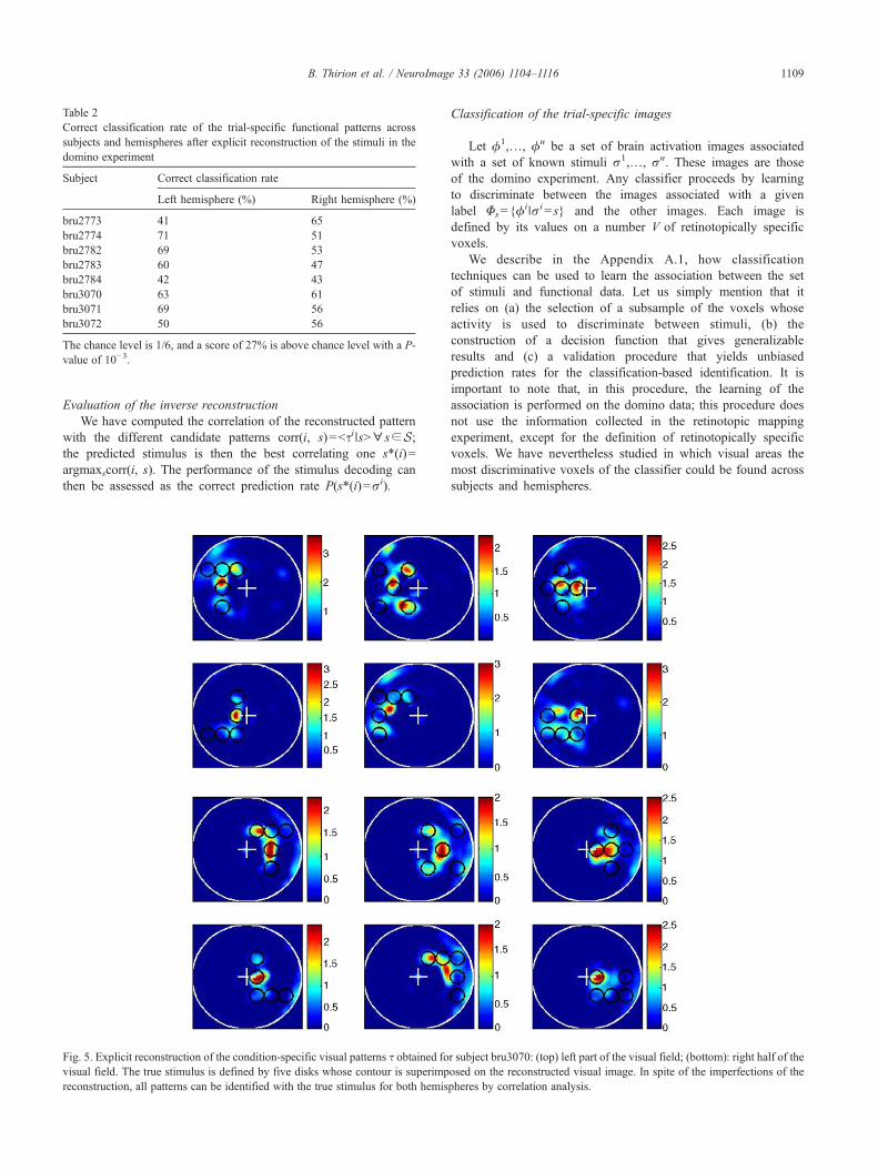
Table 2Correct classification rate of the trial-specific functional patterns acrosssubjects and hemispheres after explicit reconstruction of the stimuli in thedomino experiment

Subject Correct classification rate

Left hemisphere (%) Right hemisphere (%)

bru2773 41 65bru2774 71 51bru2782 69 53bru2783 60 47bru2784 42 43bru3070 63 61bru3071 69 56bru3072 50 56

The chance level is 1/6, and a score of 27% is above chance level with a P-value of 10−3.


Evaluation of the inverse reconstructionWe have computed the correlation of the reconstructed pattern

with the different candidate patterns corr(i, s)=<τi∣s>∀ s∈S;the predicted stimulus is then the best correlating one s*(i)=argmaxscorr(i, s). The performance of the stimulus decoding canthen be assessed as the correct prediction rate P(s*(i)=σi).

Fig. 5. Explicit reconstruction of the condition-specific visual patterns τ obtained fovisual field. The true stimulus is defined by five disks whose contour is superimpreconstruction, all patterns can be identified with the true stimulus for both hemis

Classification of the trial-specific images

Let ϕ1,…, ϕn be a set of brain activation images associatedwith a set of known stimuli σ1,…, σn. These images are thoseof the domino experiment. Any classifier proceeds by learningto discriminate between the images associated with a givenlabel Φs={ϕ

i∣σi= s} and the other images. Each image isdefined by its values on a number V of retinotopically specificvoxels.

We describe in the Appendix A.1, how classificationtechniques can be used to learn the association between the setof stimuli and functional data. Let us simply mention that itrelies on (a) the selection of a subsample of the voxels whoseactivity is used to discriminate between stimuli, (b) theconstruction of a decision function that gives generalizableresults and (c) a validation procedure that yields unbiasedprediction rates for the classification-based identification. It isimportant to note that, in this procedure, the learning of theassociation is performed on the domino data; this procedure doesnot use the information collected in the retinotopic mappingexperiment, except for the definition of retinotopically specificvoxels. We have nevertheless studied in which visual areas themost discriminative voxels of the classifier could be found acrosssubjects and hemispheres.

r subject bru3070: (top) left part of the visual field; (bottom): right half of theosed on the reconstructed visual image. In spite of the imperfections of thepheres by correlation analysis.

Table 4Correct classification rate of the trial-specific functional patterns acrosssubjects and hemispheres in the visual stimulation experiment

Subject Correct classification rate

4 folds cross-validation LOO cross-validation

Lefthemisphere

Righthemisphere

Lefthemisphere

Righthemisphere

bru2773 81% 81% 70% 74%bru2774 77% 73% 85% 70%bru2782 78% 80% 85% 86%bru2783 92% 96% 91% 94%bru2784 83% 75% 85% 76%bru3070 81% 88% 86% 90%bru3071 93% 83% 96% 83%bru3072 72% 87% 75% 88%Means 82.5% (P<10−15) 83.4% (P<10−15)

The selection of significant features (P<0.1, FDR corrected), is followed bya linear SVM analysis. Two cross-validation methods are used, left: learn on3 sessions, then test on the fourth; right learn on all samples except one thentest on the left out sample. The chance level is 1/6, and a score of 27% isabove chance level with a P-value of 10−3.


Results

Explicit reconstruction of the visual stimuli

The reconstructed visual images τ(r) (see Explicit solution of theinverse problem) were correlated with the true stimuli, so that theprediction was the best correlated input image. Note that these are tsimages, i.e. one for each trial. The rate of correct responses is givenin Table 2 for each subject and hemisphere. This rate varies between41% and 71%, hence is significantly (P<10−11) above chance level(1/6) in all cases, in spite of significant between subject variability.

An example of the condition-specific reconstructed maps τ(r) isgiven for the two hemispheres of subject bru3070 in Fig. 5. Thecorrelation of the reconstructed visual patterns with the differentcandidate shapes is given in Table 3 for this subject. Although themost lateral part of the stimulus was imperfectly inferred, thisreconstruction allows for an unambiguous recognition of the truestimulus in both hemispheres.

For comparison, the reconstructed images and correlation withthe candidate patterns are given as Supplementary Fig. 1 and Table 1for subject bru3071. In general, the images reconstructed from theother data sets have similar quality and correlation scores. Theaverage of the correlation scores across all subjects is given inSupplementary Table 2.

We have also performed the reconstruction of the stimulus usingonly voxels from area V1, which has been delineated from theretinotopy experiment. This gives quite similar results as thereconstruction fromall retinotopic voxels, in terms of visual appearanceand in terms of correlation. Reconstructed images and a correlationtable with the candidate patterns are provided as Supplementarymaterial Fig. 2 and Table 3 respectively for subject bru3070.

Classification of the trial-specific activation images

In the analysis of the domino experiment, we have selected thevoxels based on their ANOVA score, keeping only voxels with an

Table 3Correlation of the reconstructed pattern with the different candidate patternsfor subject 3070

Ideally, the diagonal value should be 1, and the off-diagonal values shouldbe between 0 and 0.8, reflecting the correlation between the true stimuli.In the present case, the maximal values of each row, indicated in bold font,are actually in the diagonal, within the [0.3 0.8] interval.

activity significantly modulated by the domino category (P<0.1,FDR corrected), see Appendix A.1.2. The activity of the selectedvoxels is the input to a linear SVM classifier. Table 4 presentsresults with two different cross-validation schemes: on the left partof the table, three sessions (108 trials, see section Stimuli) are usedas the training samples and the fourth session (36 trials) as theindependent test set. This procedure is repeated four times andclassification rate is averaged across the four runs. On the right partof the table, we performed a Leave-One-Out (LOO) procedurewhere all samples except one are used to train the discriminantmodel, which is then tested against the left-out sample. Weobtained between 70% and 96% correct classification, according tothe subject and the hemisphere. All 16 data sets were classifiedsignificantly (P<10−11) above the chance level (1/6 or 16.7%correct responses).

Across subjects and hemispheres, we found that 50–60% of themost discriminative voxels were in V1, while only 20% were in V2(ventral and dorsal). We did not try to study other visual areas,since their delineation was not reliable enough from our retinotopicmaps.

Mental imagery: explicit reconstruction of the patterns

The imagery activation images were also submitted to the inversereconstruction procedure. We have tried to identify the pattern thatwas imagined by the subject using separately the data from the leftand right hemisphere using condition-specific activation images, i.e.the images being averaged across trials, and trial-specific activationimages. An example of condition-specific reconstructed pattern isgiven in Fig. 6, together with its correlation with he correlations withthe candidate shapes.

In five out sixteen hemispheres (bru2774, right, bru2783, right,bru3070, right, bru3071, left, bru3072, left ), we were able topredict the stimulus that the subject had imagined – or reported toimagine–by correlation of the reconstructed pattern with thecandidate patterns.

On a trial-by trial basis, we were able (i) to identify the laterality(left or right hemifield) of the imagined pattern with significant

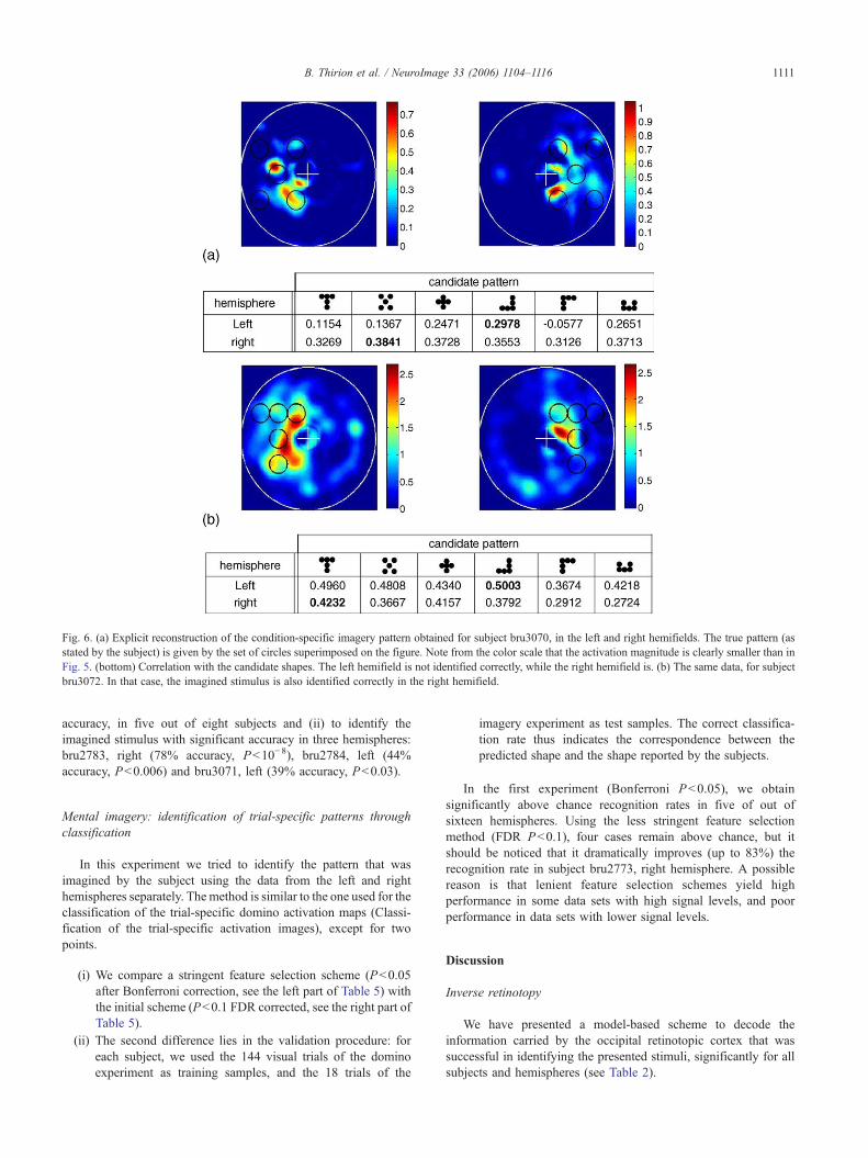
Fig. 6. (a) Explicit reconstruction of the condition-specific imagery pattern obtained for subject bru3070, in the left and right hemifields. The true pattern (asstated by the subject) is given by the set of circles superimposed on the figure. Note from the color scale that the activation magnitude is clearly smaller than inFig. 5. (bottom) Correlation with the candidate shapes. The left hemifield is not identified correctly, while the right hemifield is. (b) The same data, for subjectbru3072. In that case, the imagined stimulus is also identified correctly in the right hemifield.


accuracy, in five out of eight subjects and (ii) to identify theimagined stimulus with significant accuracy in three hemispheres:bru2783, right (78% accuracy, P<10−8), bru2784, left (44%accuracy, P<0.006) and bru3071, left (39% accuracy, P<0.03).

Mental imagery: identification of trial-specific patterns throughclassification

In this experiment we tried to identify the pattern that wasimagined by the subject using the data from the left and righthemispheres separately. The method is similar to the one used for theclassification of the trial-specific domino activation maps (Classi-fication of the trial-specific activation images), except for twopoints.

(i) We compare a stringent feature selection scheme (P<0.05after Bonferroni correction, see the left part of Table 5) withthe initial scheme (P<0.1 FDR corrected, see the right part ofTable 5).

(ii) The second difference lies in the validation procedure: foreach subject, we used the 144 visual trials of the dominoexperiment as training samples, and the 18 trials of the

imagery experiment as test samples. The correct classifica-tion rate thus indicates the correspondence between thepredicted shape and the shape reported by the subjects.

In the first experiment (Bonferroni P<0.05), we obtainsignificantly above chance recognition rates in five of out ofsixteen hemispheres. Using the less stringent feature selectionmethod (FDR P<0.1), four cases remain above chance, but itshould be noticed that it dramatically improves (up to 83%) therecognition rate in subject bru2773, right hemisphere. A possiblereason is that lenient feature selection schemes yield highperformance in some data sets with high signal levels, and poorperformance in data sets with lower signal levels.

Discussion

Inverse retinotopy

We have presented a model-based scheme to decode theinformation carried by the occipital retinotopic cortex that wassuccessful in identifying the presented stimuli, significantly for allsubjects and hemispheres (see Table 2).

Table 5Correct classification rate of the 18 trials of the imagery experiment, using adiscriminant model built on the 144 trials of the domino experiment of thecorresponding subject and hemisphere

Subject Correct classification rate computed by LOO (P-value)

Bonferroni P<0.05 FDR P<0.1

Lefthemisphere

Righthemisphere

Lefthemisphere

Righthemisphere

bru2773 11% (0.83) 44% (0.005) 11% (0.83) 83%(1.04e−9)

bru2774 28% (0.17) 0% (0.96) 17% (0.6) 0% (0.96)bru2782 33% (0.07) 17% (0.6) 17% (0.6) 17% (0.6)bru2783 0% (0.96) 6% (0.96) 0% (0.96) 11% (0.83)bru3070 67%

(2.19e−5)40% (0.03) 73%

(1.94e−6)20% (0.47)

bru3071 0% (0.96) 11% (0.83) 0% (0.96) 6% (0.96)bru3072 50%

(1.13e−3)38% (0.02) 44%

(5.3e−3)39% (0.02)

The left and right parts of the table differ on the feature selection method.Each rate is given with P-values computed relative to the null hypothesisthat the classifier was operating at chance level. Significantly greater thanchance results are emphasized with a bold font. Non-significant results are ingrey. The chance level is 1/6, and a score of 33% is above chance level with aP-value of 0.05.


These results confirm that (i) retinotopic activations in theprimary visual cortex are reproducible across trials and sessions,(ii) the retinotopic information obtained with the now classicaltraveling wave paradigm (Engel et al., 1997) can be used as a code,as suggested in (Tootell et al., 1998b; Vanni et al., 2005), and (iii) alinear filter model for V1 (Hansen et al., 2004), that we use in ourforward model, holds as a first approximation.

An important new feature of our approach compared to recentcontributions (Haynes and Rees, 2005; Kamitani and Tong, 2005)is that we compare classification techniques that model implicitlythe stimulus/activation relationship with the explicit resolution ofan inverse problem. Importantly, these techniques are based ondifferent hypotheses:

• Supervised classification assumes that reproducible differencesmight be found between functional images, so that theassociated stimulus can be inferred. The important issue is toidentify and select the discriminating information and to assessits reliability. Cross-validation and heuristic arguments are usedto solve the problem. The acquired knowledge is restricted to thecategories presented in the learning set.

• Inverse reconstruction builds on a model of the activationprocess, with explicit simplifying assumptions. The main issueis to find a simplified model that remains consistent with thedata. The inverse problem can then be solved in a rathersystematic way, and with any kind of input data: the initialretinotopic mapping is assumed here to yield a generalizablemodel of any visual activation.

As we have noticed, SVM-based classification yields moreaccurate results than the inverse problem; the price to pay is that itis not as general. But a key point is that the high performance ofclassifiers indicates that sufficient discriminant information isindeed present in the data, even if it was not explicitly decoded:some identification failures in the inverse problem can thus beattributed to shortcomings of the model rather than insufficient

information in the data (which might e.g. be related to theperformance or attention of the subjects).

Mental imagery

Moreover, we were able to extrapolate our predictions frompassive viewing experiments to mental imagery in some of thesubjects, with particularly strong evidence when using classifica-tion tools. These latter findings are consistent with the hypothesisthat mental imagery involves activation in the primary visual areas,and that the spatial structure of these activations is accounted forby standard retinotopic mapping (Kosslyn et al., 1999; Klein et al.,2004; Slotnick et al., 2005).

If inter-subject differences play a mild role in the performanceof inverse retinotopy algorithms applied to actual visual stimuli,they might have more impact on the results of the imageryexperiment. In particular, the different subjects reported more orless subjective difficulty in the task performance, as alreadynoticed in the literature (Kosslyn et al., 1984). This is clear in Table5, where the performance in the prediction of the laterality variesstrongly across subjects. One can also notice that in O'Craven andKanwisher (2000), mental imagery activations were decoded inthree out of eight subjects. In view of this, the good performanceachieved in five hemispheres is thus an important result (ifresponses were random, the probability of obtaining significantvalues in five hemispheres would be P<0.00043). The explicitidentification of the imagined pattern is a challenging task, due tothe weak signals that are obtained (see Fig. 6). Note that, besidesthe well-known weakness of retinotopic activations in imageryexperiments (Klein et al., 2004), the subjects had to keep their eyesopen and fixate the grid during this experiment, which might havereduced the level of activation in primary visual areas.

Technical aspects

Care should be taken when evoking fMRI-based brain readingexperiments. In particular, any method rests on a deconvolution ofthe hemodynamic responses on a voxel-by-voxel basis. We haveperformed this using a standard GLM procedure, which isreasonable given that the temporal linearity hypothesis might befulfilled given our inter-stimulus intervals (6 s) (Boynton et al.,1996; Soltysik et al., 2004). One might think, however, thatunmodeled spatio/temporal interactions may be present in the data.

Another set of simplifications were introduced in our formula-tion of the forward model: linearity of the transfer operator,isotropic Gaussian receptive field (RF) structure at the voxel level,constant RF size, linear gain. While this model might be partiallysupported by current knowledge about V1 (Tootell et al., 1998b;Hansen et al., 2004), it is obviously an over-simplification(Olshausen and Field, 2005), especially if one considers highervisual areas. However, it is important to keep in mind that fMRIsignals represent in each voxel the average of the activity ofthousands of neurons, so that some hypotheses, e.g. the spatiallinearity or superposition principle used here, that are known to beviolated at a microscopic level, may hold approximately at themuch lower spatial resolution and/or using standard field strength.Clearly, our forward problem framework may be a good bench-mark to test violations of different hypotheses, e.g. the spatiallinearity of visual activity as seen in fMRI (see e.g. Shmuel et al.,2002, 2006). For instance, we have also implemented Mexican hatfilters (Laplacian of the Gaussian), but did not find significant


improvements in the results. Our interpretation is that the mainbottleneck in the forward/inverse problem is the correctness of theestimate of pv in each voxel (see Eq. (2) and Appendix A.2).Assuming that this parameter is perfectly known, modeling non-linear effects or non-isotropic and non-Gaussian Receptive fieldswould become worthwhile.

We found that a majority (50 to 60%) of the most discriminantvoxels used in the classifier were in V1, while a much smallerproportion (around 20%) were in V2. Since this delineation was notthe primary goal of our analysis, we were not sure to obtain reliableboundaries for other visual areas and did make further identificationof the discriminative information. One could indeed expect that mostof the information on the spatial layout of the stimulus would beencoded in V1. In the Supplementary material, we show thatperforming the inverse reconstruction basedonly onV1voxels yieldsa very good approximation of what is achieved when considering allthe retinotopic voxels (see Supplementary Fig. 2 and Table 3).

The inverse problem is also limited by the possibility ofevaluating correctly the precision of the results (see e.g. Eq. (12)).Approximations must be performed, so that the probabilisticinterpretation of the visual patterns is not fully assessed. For thisreason, we based our test procedure on the correlation of thereconstructed pattern with the possible candidates, rather than on afully probabilistic interpretation of the reconstructed maps.

Power and limits of inverse retinotopy

First, it should be noticed that the retinotopic mapping wasperformed in less that 20 min in each subject, so that the limitedaccuracy of the retinotopic information may be the main limit inthis experiment.

Not unexpectedly, many confusions occurred between spatialpatterns that overlapped. For instance, the -shaped and -shapedpatterns in Fig. 1(c) were often confounded. Moreover, the -shapedpattern was rarely identified in the framework of the inverseproblem: it is interesting to note that this pattern is the leastcompact. This might be attributable to the low-pass filteringinherent to the inverse problem. This effect is particularly evidentfrom Fig. 5 and Supplementary Fig. 1, and affects the results atthe group level (see Supplementary Table 2). Interestingly, the

-shaped stimulus was not confused with other patterns whenusing classification tools. Thus the problem described here might bean intrinsic shortcoming of the forward/inverse problem solution.Another important effect is that the portion of the stimulus closest tothe center of the visual field is apparently much better reconstructedthan the activity in the peripheral regions, which is often smoothedout in Fig. 5—and similarly for all the data sets studied. Thisweakness is apparently not related to the receptive field size model(see Fig. 4), and might be related to spatial/attentional modulations.For instance, the fact that left and right patterns were presentedsimultaneously facilitates fixation, but possibly increases fovealattention at the expense of the periphery. Note that this fovealemphasis effect is apparently also present in the imagery data (seeFig. 6).

Conclusion and future work

We have presented an inverse retinotopy framework that buildson two complementary points of view: an explicit inversereconstruction approach that builds on the knowledge of aretinotopic experiment to decode any activation image projected

on early visual areas, and an SVM-based classificationapproach that best classifies images into a discrete categories.We could partly extrapolate these models from passive viewingto mental imagery experiments, confirming the retinotopicnature of imagery activations. Future work might concentrateon intermediate approaches where the forward/inverse problemcould benefit from the support vector framework. Long-termresearch might address more realistic simulations of activationphenomena in the visual cortex, making the forward modelmore realistic.

Acknowledgment

We are very thankful to Jean Lorenceau, Laboratoire deNeurosciences Cognitives et Imagerie Cérébrale LENA-CNRSUPR 640, who helped us to generate the stimuli that we used in theJeda environment that he has designed, as well as for his kind andinsightful advice on retinotopic stimulation.

Appendix A

A.1. Classification of functional images withretinotopically-specific information

Let ϕ1,…, ϕn be a set of brain activation images associatedwith a set of known stimuli σ1,…, σn. Any classifier proceeds bylearning to discriminate between the images associated with agiven label Φs={ϕ

i|σi= s} and the other images. Each image isdefined by its values on a number V of retinotopically specificvoxels.

A.1.1. Multivariate analysis and the risk of overfitThe discrimination function is efficient if it combines the

information from many of these voxels: classifiers are thusinherently multivariate methods. Henceforth, we call feature avoxel-based information, sample an image of the learning or test setand label the indicator of the stimulus associated with an image.Many features, i.e. non-retinotopically specific voxels, do not carryany discriminant information, and thus they do not improve theclassifier performance. When the proportion of such useless featuresincreases, some of them are simply correlated with the associatedlabel within the training set by chance, and their information cannotgeneralize to another set of samples (test samples). Those fakepositives may dramatically harm the classifier performance. Thisproblem, known as the curse of dimensionality, is illustrated in Fig.7. The number N of features increases along the horizontal axis, so

that the rationN

decreases: the training space becomes sparser. As

shown by the blue line, the classifier rapidly reaches 100% of correctrecognition on the training samples. In parallel, the performance ofthe classifier on an independent test set of images increases until itreaches a maximum of 86% recognition for N=150 as shown by thered line. Then it starts to decrease as N further increases.

To overcome this problem, we first apply a feature selection(described in Appendix A.1.2); the selected features are then givenas input to a linear Support Vector Machines (SVM) classifier,presented in Appendix A.1.3.

A.1.2. Classification step one: feature (voxels) selectionFeature selection is a crucial step of classification: it improves

the generalization power of a classifier and it is also useful to select

Fig. 7. Recognition rate (evaluated by a Leave-One-Out scheme) as afunction of the number of input features (voxels) for the subject bru2782, lefthemisphere. We measure the recognition rate of the classifier on the trainingset and on an independent test set when the number N of input features variesfrom 1 to 800.


a small subset of discriminant features, which is a requirement tointerpret results in biological applications such as neuroscience oreven genomics. Among feature selection methods (Guyon andElisseeff, 2003), we choose a supervised univariate method basedon the computation of an ANOVA F and P-values. This simplefeature selection approach belongs to the family of methods calledfilters. Filters are supervised univariate methods that rank featuresindependently of the context of others features, according to theirability to separate the populations. Such methods are computa-tionally efficient, which makes them tractable even on thousands offeatures as in our case. Unlike PCA, filters select the features in theoriginal feature space which eases the interpretation in terms ofdiscriminant information; moreover, these methods are less proneto overfitting than multivariate selection methods in general.

We first perform an ANOVA to compute to which extent thefeatures are label-related; this yields an F and a P-value. We selectthe features with two different methods for the control of falsepositives.

In the first case, we select significant features (P<0.05) after aBonferroni correction. When doing so, we have a strong controlof the type I error (the number of false positives) selecting fewbut reliable voxels which minimize the risk of overfit. We usethis very stringent method in difficult problems like mentalimagery (Mental imagery: identification of trial-specific patternsthrough classification).

In the case of visual stimulation (trial-specific images of thedomino experiment, see the results in Classification of the trial-specific images), the risk of overfit is lower. Hence we want toreduce the type II error in order to grab more discriminant featuresas input of the classifier. Thus we select significant features(P<0.1) after a False Discovery Rate (FDR) (Benjamini andHochberg, 1995) correction.

A.1.3. Classification step two: linear SVMSupport Vector Machines (SVMs) (Schölkopf and Smola,

2002) have recently been successfully used in fMRI applications(Cox and Savoy, 2003; LaConte et al., 2005; Kamitani and Tong,2005). Briefly speaking SVMs build their discriminant model as alinear combination of critical training samples. Those samplescalled Support Vectors (SVs) are either samples that lie close tothe boundary of the two classes or samples that cannot be

correctly classified. The success of SVMs on real data may beexplained by their design which properly deals with few samplesin high dimensional spaces: in a N-dimensional space with nsamples, SVMs are fully parameterized with n+1 parameters,while e.g. Linear Discriminant Analysis requires the estimation ofN(N+3) /2 parameters. This simple fact may explain the goodbehavior of SVMs in high dimensional spaces. Another argumentis that the SVM model enhances the parsimony of thediscriminant model: SVMs not only attempt to perform a goodclassification of the training samples, as a perceptron algorithmdoes, but also constrain the discriminant model to be as simple aspossible, i.e. a model in which the number of SVs is minimal.The choice of a linear SVM instead of a radial SVM (Schölkopfand Smola, 2002) has been done after simple experimentsconducted on one of the subjects (bru2782, left hemisphere),without any feature selection procedure. The linear SVM reaches62% of correct classification while the radial SVM only reaches22%. It is noticeable that the superiority of linear SVM has alsobeen reported in Cox and Savoy (2003). The cost parameter(Schölkopf and Smola, 2002) of the linear SVM has been set to 1and the implementation comes from LIBSVM (http://www.csie.ntu.edu.tw/~cjlin/libsvm).

A.1.4. ValidationValidation is a simple but crucial point that must be carefully

conducted in order to assess the quality of a discriminant modelwithout any methodological bias. The classical way is to performan out-of-sample validation which consists of: (i) setting aside anindependent set of subjects (the test set), (ii) learning on theremaining subjects (the training set) and (iii) testing thediscriminant model on the test set. Cross-validation or bootstrapvalidation repeats the previous procedure and averages the errorson test sets. The limit case of cross-validation is the Leave-One-Out procedure where only one subject is set aside. It should benoticed that feature selection is the first step of the discriminantmodel, thus it must be performed within the cross-validation loop,only on the training samples, and not as a pre-processing on allsamples before the cross-validation.

A.2. Analysis of the retinotopic maps: estimation of pv

We detail here how the voxel-based time courses during theretinotopy experiment can be used to infer the center pv of thereceptive field associated with any voxel v. Note that this is thestandard procedure used to analyze retinotopic mapping experi-ments (see e.g. Sereno et al., 1995).

Let ϕi(v), i=1: n be the values of the fMR images at voxel vduring one retinotopic mapping session (e.g. the clockwise rotatingwedge). The stimulation is periodic with a period T0=32 s, i.e. a

rotation speed x0 ¼ 2pT0

. Fourier analysis of ϕi(v) yields

ϕiðvÞ ¼ AðvÞcosðx0i� hðvÞÞ þ wi ð16Þ

where A(v)>0 is an estimate of the amount of activity at frequencyx0

2pin ϕi(v), θv the phase associated with voxel v and w the

unmodeled signal. Note that the estimation of (A(v), θ(v)) can becast in the framework of the general linear model since Eq. (16) isequivalent to

ϕiðvÞ ¼ A1ðvÞcosðx0iÞ þ A2ðvÞsinðx0iÞ þ wi ð17Þ

http://www.csie.ntu.edu.tw/~cjlin/libsvm

http://www.csie.ntu.edu.tw/~cjlin/libsvm


where A1(v)=A(v) cos(θ(v)) and A2(v)=A(v) sin(θ(v)). Thisenables us to use standard high-pass filtering and AR(1) residualwhitening that are commonly used in fMRI data analysis(Ashburner et al., 2004). Note that Eqs. (16)–(17) rest on anapproximation in which only the fundamental frequency of thestimulus is considered. Although we have also used morecomplete models of the retinotopic activity, there was littledifference regarding the estimation of θ(v), which is ultimately theparameter of interest.

Before turning to the analysis of the phase information, let usfirst notice that the assessment through a standard Fisher statisticthat ||A(v)||2 >0 yields retinotopically specific voxels.

Then θ(v)∈ [−π, π] measures the delay of ϕv with respect to theactivity in a reference region, which is equal to the polar anglebetween pv and the reference direction, biased by an hemodynamicoffset. This offset is nicely canceled out by averaging the value ofθ(v) across both directions of phase change. We end up with anestimation of the polar angle α(v)∈ [−π, π] of pv. Similarly, theanalysis of expanding/contracting ring stimulus provides us aphase eccentricity value θv∈ [−π, π], which is not biased by thehemodynamic delay. The latter value is converted to a physical

eccentricity f vð Þ ¼ d2p

pþ h vð Þð Þ, where δ=9.5° is the maximal

visual eccentricity achieved by the stimulus.The values define uniquely an estimate pv ¼ fðvÞcosðaðvÞÞ

fðvÞsinðaðvÞÞ� �

of pv.

Appendix B. Supplementary data

Supplementary data associated with this article can be found, inthe online version, at doi:10.1016/j.neuroimage.2006.06.062.

References

Ashburner, J., Friston, K., Penny, W., 2004. Human Brain Function, 2nd Ed.Academic Press.

Benjamini, Y., Hochberg, Y., 1995. Controlling the false discovery rate: apractical and powerful approach to multiple testing. J. R. Stat. Soc. 57(1), 289–300.

Boynton, G.M., Engel, S.A., Glover, G.H., Heeger, D.J., 1996. Linearsystems analysis of functional magnetic resonance imaging in humanV1. J. Neurosci. 16, 4207–4221.

Carlson, T.A., Schrater, P., He, S., 2003. Patterns of activity in thecategorical representations of objects. J. Cogn. Neurosci. 15 (5),704–717.

Cox, D.D., Savoy, R.L., 2003. Functional magnetic resonance imaging(fmri) “brain reading”: detecting and classifying distributed patterns offmri activity in human visual cortex. NeuroImage 19 (2), 261–270.

Davatzikos, C., Ruparel, K., Fan, Y., Shen, D.G., Acharyya, M., Loug-head,J.W., Gur, R.C., Langleben, D.D., 2005. Classifying spatial patterns ofbrain activity with machine learning methods: application to liedetection. NeuroImage 28 (3), 663–668.

Dehaene, S., Clec'H, G.L., Cohen, L., Poline, J.-B., de Moortele, P.-F.V.,Bihan, D.L., 1998. Inferring behavior from functional images. Nat.Neurosci. 1 (7), 549–550.

DeYoe, E.A., Carman, G.J., P.B., Bandettini, P., Glickman, S., Wieser, J.,Cox, R., Miller, D., Neitz, J., 1996. Mapping striate and extrastriatevisual areas in human cerebral cortex. Proc. Natl. Acad. Sci. U S A 93(6), 2382–2386.

Dougherty, R.F., Koch, V.M., Brewer, A.A., Fischer, B., Modersitzki, J.,Wandell, B.A., 2003. Visual field representations and locations of visualareas V1/2/3 in human visual cortex. J.Vis. 3 (10), 586–598.

Duncan, R.O., Boynton, G.M., 2003. Cortical magnification within human

primary visual cortex correlates with acuity thresholds. Neuron 38 (4),659–671.

Engel, S.A., Glover, G.H., Wandell, B.A., 1997. Retinotopic organization inhuman visual cortex and the spatial precision of functional MRI. Cereb.Cortex 7 (2), 181–192.

Guyon, I., Elisseeff, A., 2003. An introduction to variable and featureselection. J. Mach. Learn. Res. 3, 1157–1182 (Special issue on variableand feature).

Hansen, K.A., David, S.V., Gallant, J.L., 2004. Parametric reversecorrelation reveals spatial linearity of retinotopic human V1 BOLDresponse. NeuroImage 23 (1), 233–241.

Hanson, S.J., Matsuka, T., Haxby, J.V., 2004. Combinatorial codes in ventraltemporal lobe for object recognition: Haxby (2001) revisited: is there a“face” area? NeuroImage 23 (1), 156–166.

Haxby, J.V., Gobbini, M.I., Furey, M.L., Ishai, A., Schouten, J.L.,Pietrini, P., 2001. Distributed and overlapping representations offaces and objects in ventral temporal cortex. Science 293 (5539),2425–2430.

Haynes, J.-D., Rees, G., 2005. Predicting the orientation of invisible stimulifrom activity in human primary visual cortex. Nat. Neurosci. 8,686–691.

Kamitani, Y., Tong, F., 2005. Decoding the visual and subjective contents ofthe human brain. Nat. Neurosci. 8, 679–685.

Klein, I., Dubois, J., Mangin, J.-F., Kherif, F., Flandin, G., Poline,J.-B., Denis, M., Kosslyn, S.M., Bihan, D.L., 2004. Retinotopicorganization of visual mental images as revealed by functionalmagnetic resonance imaging. Brain Res. Cogn. Brain Res. 22 (1),26–31.

Kosslyn, S.M., Brunn, J., Cave, K.R., Wallach, R.W., 1984. Individualdifferences in mental imagery ability: a computational analysis.Cognition 18 (1–3), 195–243.

Kosslyn, S.M., Pascual-Leone, A., Felician, O., Camposano, S., Keenan,J.P., Thompson, W.L., Ganis, G., Sukel, K.E., Alpert, N.M., 1999. Therole of area 17 in visual imagery: convergent evidence from PET andrTMS. Science 284 (5411), 167–170.

LaConte, S., Strother, S., Cherkassky, V., Anderson, J., Hu, X., 2005.Support vector machines for temporal classification of block designfMRI data. NeuroImage 26 (2), 317–329.

O'Craven, K.M., Kanwisher, N., 2000. Mental imagery of faces and placesactivates corresponding stimulus-specific brain regions. J. Cogn.Neurosci. 12 (6), 1013–1023.

Olshausen, B.A., Field, D.J., 2005. How close are we to understanding V1?Neural Comput. 17 (8), 1665–1699.

Piazza, M., Giacomini, E., Le Bihan, D., Dehaene, S., 2003. Single-trialclassification of parallel pre-attentive and serial processes usingfunctional magnetic resonance imaging. Phil. Trans. R. Soc. Lond. B.270, 1237–1245.

Rivière, D., Papadopoulos-Orfanos, D., Poupon, C., Poupon, F., Coulon, O.,Poline, J.-B., Frouin, V., Régis, J., Mangin, J.-F., 2000. A structuralbrowser for human brain mapping. In Proc. 6th HBM. NeuroImage 11(5), 912 (San Antonio, Texas).

Schölkopf, B., Smola, A., 2002. Learning with Kernels: Support VectorMachines, Regularization, Optimization, and Beyond. MIT Press,Cambridge, MA.

Sereno, M.I., Dale, A.M., Reppas, J.B., Kwong, K.K., Belliveau, J.W.,Rosen, B.R., Tootell, R.B., 1995. Borders of multiple visual areas inhumans revealed by functional magnetic resonance imaging. Science268, 889–893.

Shmuel, A., Yacoub, E., Pfeuffer, J., de Moortele, P.F.V., Adriany, G., Hu,X., Ugurbil, K., 2002. Sustained negative BOLD, blood flow andoxygen consumption response and its coupling to the positive responsein the human brain. Neuron 36 (6), 1195–1210.

Shmuel, A., Augath, M., Oeltermann, A., Logothetis, N.K., 2006.Negative functional MRI response correlates with decreases inneuronal activity in monkey visual area V1. Nat. Neurosci. 9 (4),569–577.

Slotnick, S.D., Thompson, W.L., Kosslyn, S.M., 2005. Visual mental

http://dx.doi.org/doi:10.1016/j.neuroimage.2006.06.062


imagery induces retinotopically organized activation of early visualareas. Cereb. Cortex 15 (10), 1570–1583.

Smith, A.T., Singh, K.D., Williams, A.L., Greenlee, M.W., 2001. Estimatingreceptive field size from fMRI data in human striate and extrastriatevisual cortex. Cereb. Cortex 11 (12), 1182–1190.

Soltysik, D.A., Peck, K.K., White, K.D., Crosson, B., Briggs, R.W., 2004.Comparison of hemodynamic response nonlinearity across primarycortical areas. NeuroImage 22 (3), 1117–1127.

Tootell, R.B., Dale, A., Sereno, M., Malach, R., 1996. New images fromhuman visual cortex. Trends Neurosci. 19, 481–489.

Tootell, R.B.H., Hadjikhani, N., Mendola, J.D., Marett, S., Dale, A.M.,1998a. From retinotopy to recognition: fMRI in human visual cortex.Trends Cogn. Sci. 2, 174–183.

Tootell, R.B., Hadjikhani, N.K., Vanduffel, W., Liu, A.K., Mendola, J.D.,

Sereno, M.I., Dale, A.M., 1998b. Functional analysis of primaryvisual cortex (V1) in humans. Proc. Natl. Acad. Sci. U. S. A. 95 (3),811–817.

Tootell, R.B., Tsao, D., Vanduffel, W., 2003. Neuroimaging weighs in:humans meet macaques in “primate” visual cortex. J. Neurosci. 23,3981–3989.

Vanni, S., Henriksson, L., James, A.C., 2005. Multifocal fMRI mapping ofvisual cortical areas. NeuroImage 27 (1), 95–105.

Warnking, J., Dojat, M., Guerin-Dugue, A., Delon-Martin, C., Olympieff,S., Richard, N., Chehikian, A., Segebarth, C., 2002. fMRI retinotopicmapping—step by step. NeuroImage 17, 1665–1683.

Wotawa, N., Thirion, B., Castet, E., Anton, J.-L., Faugeras, O., 2005.Human retinotopic mapping using fMRI. Technical Report 5472, INRIASophia-Antipolis.

inverse retinotopy: inferring the visual content of images from brain activation patterns

Documents