Inventory-Theoretic Model of Money Demand, MultipleGoods, and Price Dynamics

Hirokazu Ishise� Nao Sudoy

July 29, 2008

Abstract

Despite the theoretical prediction based on sticky-price models, it is empirically suggestedthat the tie between the frequencies of price adjustment across goods and the relative priceresponses of goods (price index of speci�c goods over non-durable aggregate price index) toa monetary policy change is limited.We o¤er an alternative view of the price dynamics of goods. We develop a multi-sector

extension of an inventory-theoretic model of money demand (segmented market model). Inour model, the diversity in the characteristics of goods, that is, durability, luxuriousness andcash intensity (the portion of the payment that is paid by cash in the purchase of goods),yields the dispersion of relative prices responses to a monetary policy shock, across goods.The model implies that the relative prices of durables, luxuries and less cash-intensive goodstend to decline in a monetary contraction.We test the empirical plausibility of our model, using two approaches: a measure of

monetary policy shock developed by Romer and Romer (2004), and a factor-augmented VARused in Bernanke et al. (2005). In both econometric methodologies, we �nd that the dataare consistent with our model, in terms of durability and luxuriousness.

Keywords: Baumol-Tobin model; Durable; Luxury; Credit goods; Monetary policy;

1 Introductory remarks

In the macroeconomics literature, a monetary policy e¤ect is considered to be tightly related to

prices responses to a policy change. As monetary policy focuses on the aggregate demand of an

economy, many studies, such as Rotemerg and Woodford (1997) and Goodfriend and King (1998),

regard an aggregate price index of non-durables, as a relevant price series for policy analysis.

�Department of Economics, Boston University, ishise@bu.eduyCorresponding author; Economist, Institute for Monetary and Economic Studies, Bank of Japan (E-mail:

nao.sudou@boj.or.jp). The authors would like to thank Robert King, Anton Braun, Simon Gilchrist, FrancoisGourio, Naohisa Hirakata, Takashi Kano, Masao Ogaki, Adrian Verdelhan, seminar participants at GLMM (GreenLine Macro Meeting) and the sta¤ of the Institute for Monetary and Economic Studies (IMES), the Bank of Japan,for their useful comments. Views expressed in this paper are those of the authors and do not necessarily re�ect theo¢ cial views of the Bank of Japan.

1

Recently, macroeconomists turned their attention to a more disaggregated level of prices (Bils

et al., 2003; Erceg and Levin. 2002; Barsky et al., 2007; Boivin et al., 2007). In particular,

Boivin et al. (2007) investigate the sectoral responses of prices to a monetary policy shock, using

item level of personal consumption expenditure (PCE) data and producer price indices. They

observe a large cross-sectional dispersion across items, in the way the prices of those items respond

to a monetary policy shock. That is, relative prices across goods change drastically following a

monetary policy shock. For example, they report clear heterogeneity in price responses betweem

durables and non-durables. Other studies focus on more aggregated prices, and �nd a similar

pattern of heterogeneity across sectors.

To examine this heterogeneity more closely, we estimate the impulse response functions (IRFs)

of prices to a contractionary monetary policy shock, for 189 PCE items. IRFs are calculated

using the approach of Romer and Romer (2004) (see Appendix B for details). For convenience of

analysis, we normalize each of the price indices by an aggregate non-durables price index. Table 1

reports the number of prices that either rise or decline signi�cantly, with respect to the aggregate

non-durables price index, after a monetary policy shock1. Among 189 items, the relative prices rise

for 15 items, while for 62 items, the relative prices decline signi�cantly. Among durables, relative

prices decline for more than half of the items.

(Table 1)

(the number of items whose relative prices either rises or declines)

All Items Rise 15 items

(189 items) Decline 62 items

Durables Rise 0 items

(30 items) Decline 17 items

Non­durables Rise 15 items

(159 items) Decline 45 items

The mechanism that produces the cross-sectional di¤erences in the relative prices is not well

understood so far. In the sticky-price framework, a dispersion in the frequency of price adjustments

across sectors operates as a strong mechanism that yields the cross-sectional di¤erences in price

responses to a shock. In the multi-sector extension of the sticky-price model (see, for example,

Ohanian et al., 1995; Carvalho, 2006), sectors that adjust prices frequently coexist with those that

adjust them infrequently. Prices in the former respond faster to a monetary policy shock, than

those in the latter, leading to a short-run change in the relative price of the two goods.

It is observed, however, that the actual price dynamics of goods are not closely linked to the

frequency of price adjustments of goods (Bils et al., 2003; Bils and Klenow, 2004). Following

Christiano et al. (1999), Bils et al. (2003) estimate the empirical responses of goods prices to

1To determine the signi�cance, we calculate the 10% con�dence interval. The prices of the items are consideredto be signi�cantly rising (or declining), if there is at least a month when the lower (upper) bound of the con�denceinterval crosses zero within a two-year horizon.

2

a monetary policy shock, to observe the inconsistency between the data and the prediction of

the sticky-price model. They �nd that the relative price of �exible-price goods, with respect to

sticky-price goods, descends following a monetary expansion shock.

The weakness of the link can also be seen by a di¤erent approach. We �rst estimate the

cumulative impulse response (CIRs) of the relative prices of PCE items to a monetary policy

shock, using two recently developed econometric procedures. One is a regression using a measure

of monetary policy shock provided in Romer and Romer (2004). The other is the factor-augmented

VAR (FAVAR), developed in Bernanke et al. (2005), and applied to disaggregated price analysis

in Boivin et al. (2007) (see Section 4 and Appendix B for details). We then regress each of the

estimated CIRs of the PCE items on the frequencies of price adjustment of goods that are reported

in Nakamura and Steinsson (2007)2, to see the tie.

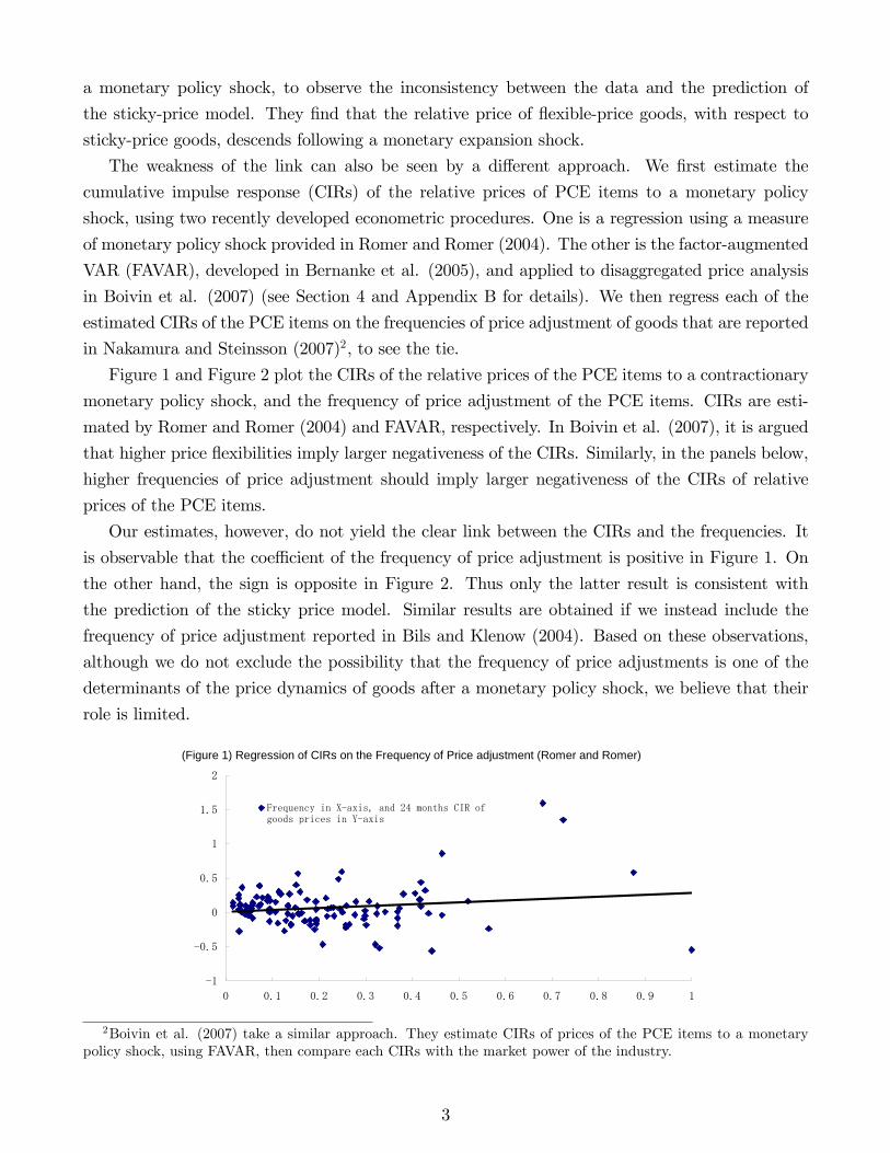
Figure 1 and Figure 2 plot the CIRs of the relative prices of the PCE items to a contractionary

monetary policy shock, and the frequency of price adjustment of the PCE items. CIRs are esti-

mated by Romer and Romer (2004) and FAVAR, respectively. In Boivin et al. (2007), it is argued

that higher price �exibilities imply larger negativeness of the CIRs. Similarly, in the panels below,

higher frequencies of price adjustment should imply larger negativeness of the CIRs of relative

prices of the PCE items.

Our estimates, however, do not yield the clear link between the CIRs and the frequencies. It

is observable that the coe¢ cient of the frequency of price adjustment is positive in Figure 1. On

the other hand, the sign is opposite in Figure 2. Thus only the latter result is consistent with

the prediction of the sticky price model. Similar results are obtained if we instead include the

frequency of price adjustment reported in Bils and Klenow (2004). Based on these observations,

although we do not exclude the possibility that the frequency of price adjustments is one of the

determinants of the price dynamics of goods after a monetary policy shock, we believe that their

role is limited.

(Figure 1) Regression of CIRs on the Frequency of Price adjustment (Romer and Romer)

­1

­0.5

0

0.5

1

1.5

2

0 0.1 0.2 0.3 0.4 0.5 0.6 0.7 0.8 0.9 1

Frequency in X­axis, and 24 months CIR ofgoods prices in Y­axis

2Boivin et al. (2007) take a similar approach. They estimate CIRs of prices of the PCE items to a monetarypolicy shock, using FAVAR, then compare each CIRs with the market power of the industry.

3

(Figure 2) Regression of CIRs on the Frequency of Price adjustment (FAVAR)

­5

­4

­3

­2

­1

0

1

2

3

4

5

6

0 0.1 0.2 0.3 0.4 0.5 0.6 0.7 0.8 0.9 1

Frequency in X­axis,and 12 months CIR ofgoods prices in Y­axis

To answer to the same question, but from a di¤erent perspective, we develop an inventory-

theoretic model of money demand. The classic works on the inventory-theoretic model by Baumol

(1952) and Tobin (1956) are extended, following the subsequent works by Grossman and Weiss

(1983) and Alvarez et al. (2003), so that we are able to analyze the e¤ect of a monetary policy

shock on the price responses of various goods. In our economy, no friction associated with price

settings is assumed. We instead assume a friction in accessing the �nancial market. We consider

an economy where the �nancial market and the goods market are separated, and access to the

�nancial market incurs costs on households3. Given this access cost, households withdraw money

from banks infrequently, and they spend the money over several periods. Because only a portion of

money present in the economy is used for transactions, a change in aggregate money supply is not

fully re�ected in a change in the prices of goods that are purchased during the period. Thus, in a

wake of monetary policy shock, such as an exogenous fall in money supply, prices adjust sluggishly.

In order to discuss the relative price of goods in the inventory-theoretic framework, we incor-

porate the multiple-goods set up used in Bils and Klenow (1998). Using standard consumption

theory, Bils and Klenow (1998) ask if the dispersions of the cyclicality of consumption goods can be

attributed to the characteristics of goods. They �nd that �durability�and �luxuriousness�make

the responses of goods to aggregate shocks more cyclical. Following their approach, we analyze

the tie between the characteristics of goods and the price responses of goods to a monetary policy

shock. In addition to �durability�and �luxuriousness�, we study the implication of �cash goods

vs credit goods�distinction, for the price response to a monetary policy shock. Existing monetary

models, including Lucas and Stokey (1987) and Hodrick et al. (1991), classify goods by the way

of settlement. In these studies, goods paid for by cash are called cash goods, and goods paid for

by private credit are called credit goods. We follow their approach, and describe the goods that

3In the literature, there are various ways of modeling the current type of �nancial frictions. Grossman and Weiss(1983) and Alvarez et al. (2003) assume a Taylor type of �nancial friction. In these models, households are allowedto access the �nancial market every N periods, where N exogenous. In Chiu (2005) and Khan and Thomas (2007),N is endogenously determined by households. We follow the former approach.

4

are paid for by cash as cash-intensive goods.

Based on the current model, the price responses of goods to a monetary policy shock are linked

to the characteristics of the goods. Similarly to the model of Alvarez et al. (2003), we assume that

all the goods are endowed exogenously, and the prices of goods are determined by the households�

consumption decisions. In the economy, as households di¤er from each other in their timing of

access to the �nancial market, the impact of a policy shock is not uniform among them. Some

types of households become richer, and others become poorer, as a consequence of a monetary

policy shock. The equilibrium relative prices of each goods to the shocks are thus determined by

the consumption decisions by each type of households, and the relative importance of the speci�c

types.

From the simulation exercises that investigate a tie between goods�characteristics and relative

price responses of goods to a monetary policy shock, we �nd that the relative prices of durables,

luxuries and credit goods tend to descend (ascend), following a contractionary (expansionary)

monetary policy shock. This observation is invariant to the various speci�cations of the parameters

associated with the size of the �nancial frictions, or law of motion of the money supply shock.

We then investigate the plausibility of our theoretical results using the U.S. data. For each

of the PCE items, we estimate the responses of the relative prices of goods, with respect to the

aggregate price index of non-durables, to a monetary policy shock, using a measure of monetary

policy developed by Romer and Romer (2004), and the factor-augmented VAR. We test whether

the size and the sign of the estimated responses are related to the depreciation rate, luxuriousness

and cash intensity of the items, in the manner that our theory suggests. We �nd from the data

analysis that the depreciation rate and luxuriousness are the important determinants of the price

responses of goods after a monetary policy shock.

The rest of the paper is organized into four sections. Section 2 describes our model� inventory-

theoretic model with multiple consumption goods. Section 3 demonstrates how the characteristics

of goods� durability, luxuriousness and cash intensity of the goods� a¤ect price responses of the

goods to a monetary policy shock. Section 4 presents an empirical observation on the price

responses of goods to a monetary policy shock. Section 5 concludes.

2 The Model

2.1 Environment

We consider an economy where j = 1; :::; J consumption goods, and s = 0; : : : ; N � 1 equallydivided types of agents are present. We assume that the J items may be di¤erent from each other,

in terms of durability, cash intensity of payment, and luxuriousness. We say that an item jA is

5

more durable than an item jB when the depreciation rate of the item �jA 2 [0; 1] is smaller than�jB 2 [0; 1] : Similarly, we de�ne the cash intensity of payment for an item j; by a size of the

portion of the payment that households pays by cash for the purchase of the item �j 2 [0; 1] : Wede�ne luxuriousness by the income elasticity, following the terminology used by Bils and Klenow

(1998). We will see that the income elasticity is governed by the parameter �j > 0 in the utility

function. For simplicity of analysis, we treat an item j = 1 as numeraire, and we assume that the

depreciation rate, cash intensity and �j are all unity for the numeraire:

A coalition is characterized by the initial period type and each fraction consists of 1=N measure

of people. In each period, agent moves forwardly: type 0 becomes type 1, type 1 to type 2, ...,

and type N � 1 to type 0. The economy is composed of the two separate markets, and eachagent has an account for each market. One market is the �nancial market where agents trade

interest-bearing assets. Following Alvarez et al. (2003), we call the accounts used for the market

as �brokerage accounts.�The other market the a goods market where agents trade goods, and the

accounts associated with this market are named �bank accounts.�The two types of accounts are

segmented from each other, in the sense that only type s = 0 agent can rebalance assets between

the two accounts. When type s = 0 agents access their brokerage account, they transfer a nominal

money, xt, from the brokerage account to the bank account. The money in the bank account serves

to the purchase of goods in the goods market. Once they have rebalanced their assets, the agents

s = 0 need another N � 1 months before the next rebalancing.The supply side of our model is comparatively simple. In each period, every agent, type

s = 0; : : : ; N � 1 receives an equal amount of endowments for goods j, for j = 1; :::; J . Each

household is divided into shopper-saler pair, so that they cannot consume their own endowments.

Agents purchase goods either by cash or by credit or both. The payments for the purchases of

goods are deducted from the bank account if they are paid by cash, and from the brokerage account

if they are paid by credit. Earnings from selling their endowments are transferred to the accounts.

Following Alvarez et al. (2003), we assume that of the payments for goods that are settled by cash,

a portion 2 [0; 1] of the payment is sent to the bank account, and the rest of the payment is sentto the brokerage account. All the payments via credit are transferred to the brokerage account.

2.2 Households problem

Each type of agent maximizes utility over the stock of goods, kj for j = 1; :::; J . Utility function

satis�es standard increasing and diminishing marginal utility condition, ukj ! 1 if kj ! 0 for

j = 1; :::; J :1Xt=0

Xht

�t Pr(ht)u(k1;t(s; ht); :::kJ;t(s; h

t)); (1)

where ht is the history to date t, Pr(ht) is the probability of realizing a particular history of

the economy and Pr(htjht�1) is the conditional probability of reaching ht given ht�1.

6

Following Bils and Klenow (1998), we assume that the temporal utility function has the fol-

lowing addilog form:

u(k1;t(s; ht); ::kJ;t(s; h

t)) =XJ

j=1�jkj;t(s; h

t)1��j � 11� �j

; (2)

wherePJ

j=1 �j = 1, and �j stands for the steady state expenditure share of the goods j over the

consumption basket. A goods-speci�c income elasticity for goods j is captured by the intertemporal

elasticity parameter �j; as in Bils and Klenow (1998). The law of motion for the durable stock of

goods j, kj;t (s; ht) held by type s agent at period t is:

kj;t(s; ht) � [1� �j]kj;t�1(s� 1; ht�1) + cj;t(s; ht): (3)

where �j 2 [0; 1] denotes the goods-speci�c depreciation rate, and cj;t(s; ht) is the amounts ofgoods j that are purchased by agent s at the period t: For any goods j; all agents receive an equal

amount of endowment yj;t(ht) in each period. cj;t(s; ht) does not need to be equalized to yj;t(ht);

because cj;t(s; ht) is an endogenous variable while yj;t(ht) is an exogenous variable.

Households face a cash-in-advance constraint (or �bank account�constraint) and cash holding

transition:

JXj=1

�jPj;t(ht)cj;t(s; h

t) + Zt(s; ht) =Mt(s; h

t); (4)

Mt(s; ht) = Zt�1(s� 1; ht�1) +

JXj=1

�j jPj;t�1(ht�1)yj;t�1(h

t�1) + 1 � Pt(ht)xt(ht) (5)

where �j 2 [0; 1] denotes the goods-speci�c cash intensity, and Mt(s; ht) are the cash holdings

in the bank account that belong to type s at period t: (4) denotes the way cash holdings by

households of type s at period t; Mt(s; ht); are spent. In each period t; households of type s spend

a portion of their cash holdings for the purchasing of goods (the �rst term on the left-hand-side

(LHS) of (4)); and carry the rest of their money, Zt(s; ht); in the bank accounts to period t + 1:

(5) indicates the various components that constitute a cash holding at period t; Mt(s; ht): Namely,

Mt(s; ht) is the sum of (i) money that is carried by type s� 1 at period t� 1; from the previous

period, which is Zt�1(s � 1; ht�1), (ii) a portion of their earnings from selling their endowments

that are deposited in their bank accounts (the second term on the right-hand-side (RHS) of (5)),

and (iii) a transfer of cash from their brokerage account, Pt(ht)xt(ht): Note that 1 is an index

function taking 1 if s = 0 and 0 otherwise.

7

A brokerage account constraint is described as follows:

Xht+1

qtt+1(ht+1)Bt(s; h

t+1) + At(s; ht) + 1 � Pt(ht)xt(ht) +

JXj=1

[1� �j]Pj;t(ht)cj;t(s; ht)

= Bt�1(s� 1; ht) + At�1(s� 1; ht�1) +JXj=1

�j�1� j

�Pj;t�1(h

t�1)yj;t�1(ht�1)

+JXj=1

[1� �j]Pj;t(ht)yj;t(ht)� Pt(ht)� t(ht); (6)

where Bt(s; ht+1) is the amount of bond holdings of the households of type s at t, qtt+1(ht+1) is

the price of a one-period-ahead bond returning one dollar, and At(s; ht) is the cash holding at the

brokerage account. This equation shows how the assets belonging to the households of type s at

period t are accumulated. Note that a fraction of the payments for purchasing goods j that are

paid for by credit, [1� �j]Pj;t(ht)cj;t(s; ht); is deducted directly from the brokerage account, while

the rest of the payments are deducted from the bank account. The earnings from selling their

endowments of goods j, �j�1� j

�Pj;t�1(h

t�1)yj;t�1(ht�1) and [1� �j]Pj;t(ht)yj;t(ht); �ow into the

brokerage account at each period. � t(ht) is the lump-sum transfer by the government.

In addition to the accounts, households face nonnegativity constraints of Zt(s; ht), Mt(s; ht),

At(s; ht). As for the purchase of goods cj;t(s; ht) for j = 1; :::J , we assume the nonnegativity

constraint:

cj;t�s; ht

�� 0 (7)

The government faces the following government budget constraint:

Bt�1(ht) =Mt(h

t)�Mt�1(ht�1) + Pt(h

t)� t(ht) +

Xht+1

qtt+1(ht+1)Bt(h

t+1); (8)

where Mt(ht) and Bt(ht) are the average values of money and bonds in the economy, respectively.

We also de�ne the growth rate of money by �t = Mt=Mt�1. We assume �t follows a stationary

AR(1) process, where �M 2 (0; 1] :

�t = �M�t�1 + "t: (9)

Asset prices are related to nominal interest rate as follows.

1

1 + it(ht)=Xht+1

qtt+1(ht+1): (10)

8

The velocity of money circulation, vt(ht), is

vt(ht) =

1N

PJj=1 Pj;t(h

t)PN�1

s=0 cj;t(s; ht)

Mt(ht): (11)

De�nition: A Competitive Equilibrium of the Economy is

a sequence of prices ffPj;t(ht)gJj=1 ; qtt+1(ht+1)g1t=0 andthe allocations fffcj;t(s; ht); kj;t(s; ht)gJj=1 ; xt(ht); Bt(s; ht+1); At(s; ht);Mt(s; h

t); Zt(s; ht)gN�1s=0 g1t=0

for a given government policy f� t(ht);Mt(ht); Bt(h

t)g1t=0, endowment process ffyj;t(s; ht)gJj=1g1t=0

and initial conditions ffkj;�1(s� 1)gJj=1 ; B�1(s�1; :); A�1(s�1; :); Z�1(s�1; :)gN�1s=0 such that for

all t; ht :

(i)household maximizes utility given the prices;

(ii)the government budget constraint holds;

(iii)markets clear:

1

N

Xs

cj;t(s; ht) = yj;t(h

t) for j = 1; ::J (12)

1

N

Xs

Bt(s; ht+1) = Bt(h

t+1) (13)

1

N

Xs

[Mt(s; ht) + At(s; h

t)] =Mt(ht): (14)

Following Alvarez et al. (2003), we focus on an economy with a positive interest rate, so that

At(s; ht) = Zt(N � 1; ht) = 0. The endowment process is assumed to have no trend growth. We

use a log-linearized rational expectations model to analyze the dynamics of the model. The be-

havior of the economy is described as the deviation from the following non-stochastic steady state

where all the real variables stay constant:

De�nition: Non-Stochastic Steady State of the Economy is an Equilibrium with At(s) = 0,

Zt(N � 1) = 0, such that ffcj;t(s); kj;t(s)gJj=1 ; xt; Bt(s);mt(s); zt(s);mt; fpj;tgJj=1gN�1s=0

= f�cj(s); kj(s)

Jj=1; x; B(s);m(s); z(s);m; fpjgJj=1gN�1s=0 , � =Mt=Mt�1 = � = Pt=Pt�1 and qtt+1=Pt

is constant.

2.3 How the model works

In this section, we brie�y discuss the equilibrium responses of the variables to a monetary policy

shock.

The �rst order conditions with respect to the numeraire consumption and money holdings give

9

the following Euler equations for agent s, for s = 0; :::; N � 1:

u1�s; ht

�= �Et

�u1 (s+ 1; h

t+1)

�t+1 (ht+1)

�+ Pt(h

t)�zt (s; ht); (15)

where u1 (s; ht) denotes the marginal utility for households of type s from consuming numeraire

c1 (s; ht) ; and �zt (s; h

t) is the Lagrange multiplier associated with nonnegativity of Zt(s; ht)4. Etdenotes expectation conditional on time t information.

Similarly to the model of Alvarez et al. (2003), the cash-in-advance constraint is binding for

transactions in the goods market, and the consumption growth rate is a function of the price

growth rate �t+1. The equilibrium levels of money holdings by households are determined, so as to

be consistent with the growth rate of their numeraire consumption. At each period, a portion of

the households�money holdings Zt(s; ht) for s = 1; :::; N � 1 is not used for goods purchasing andis carried over to the next period. As rebalancing between the accounts happens only once every

N periods, money holdings for each household decline over successive periods, until they access to

their brokerage accounts again:

In this environment, a monetary policy shock, such as an unexpected exogenous change in

aggregate money supply, does not incur an immediate one-for-one rise in goods�price levels. A

change in the aggregate money supply leads to a gradual change in money that is used as a means

of exchange. Provided that supplies of goods are constant, prices adjust sluggishly.

Using (15) and (10), it is shown that the asset price in the �nancial market is determined by

the marginal utility of a dollar for households of type s = 0: Equivalently, the nominal interest

rate it is expressed as5:

1

1 + it= �Et

�u1 (0; h

t+1)

u1 (0; ht)�t+1(ht+1)

�: (16)

As only a subset of the households participate in the �nancial market, a monetary policy shock

primarily a¤ects the money holdings of the households who rebalance their assets during the period

of innovation. Suppose a monetary contraction shock occurs at period t: Households that are type

s = 0 during this period receive less money than those who were type s = 0 at period t� 1: As aconsequence, the numeraire consumptions by the active households decline at period t, because the

share of aggregate real money balances held by those households shrinks in the short run, leading

to a rise in the interest rate.

As for the substitution between goods j and the numeraire, combining the �rst order conditions

4Alvarez et al. (2003) point out that in an economy with positive in�ation, households of type s = N � 1 doesnot carry money to the next period. As the households are able to rebalance their assets between the brokerageaccount and bank account in the subsequent period, there is no incentive for them to keep their money unspent, orequivalently, leaving Z (N � 1; ht) positive.

5In order to derive the equation below, we need to impose some class of initial distribution for the bondsendowment. See Alvarez et al. (2003) for details.

10

for the numeraire and for the goods _j yields the user cost equation:

cj (s; ht)��j u1 (s; h

t) = pj;t (ht)

��ju1 (s; h

t) + [1� �j]u1 (0; ht) + �jt (s; ht)�

u1 (s; ht)

�� [1� �j]Etpj;t+1 (ht+1)(�ju1 (s+ 1; h

t+1)

u1 (s; ht)+[1� �j]rt (ht)

u1 (0; ht)

�u1 (s; ht)+�jt+1 (s+ 1; h

t+1)

u1 (s; ht)

);

(17)

where uj (s; ht) denotes marginal utility for agent s from consuming the goods j; rt (ht) is the

real interest rate measured by the numeraire, and �jt (s; ht) is the Lagrange multiplier associated

with the nonnegativity constraint. Clearly, the consumption decisions of households of type s on

goods j depend on the goods-speci�c parameters �j; �j and �j: We will see in the next section

that the impact of a monetary policy shock is not uniform across the households, depending on

what their types are at the period of the monetary policy shock. Thus the aggregate demand of

goods j is determined by both the goods-speci�c parameters and the households�type. Note that

provided that goods supply is una¤ected by a monetary policy shock in the current model, the

relative price pj;t (ht) changes so that (17) holds for every type s:

(Figure 3)

­1.2

­1.0

­0.8

­0.6

­0.4

­0.2

0.0

0.2

0.4

0 1 2 3 4 5 6 7 8 9 10

Price of Numeraire Money Velocity

(months)

­0.50

­0.40

­0.30

­0.20

­0.10

0.00

0.10

0.20

14 13 12 11 10 9 8 7 6 5 4 3 2 1 0

rou_m = 0.0 rou_m = 0.2

rou_m = 0.6

(two­year cumulative sum of  the response of numeraire cunsumption)

(type s ; a number of months it takes the households to rebalance the assets)

(Figure 4)

­3.0000

­2.0000

­1.0000

0.0000

1.0000

2.0000

3.0000

0 1 2 3 4 5 6 7 8 9 10

Relative Price of Durables Nominal Interest Rate

(months)

11

To see the quantitative implications of our model, we calculate the IRFs of certain variables

to a monetary policy shock. Alvarez et al. (2003) concentrate on how the price sluggishness is

generated through inventory-theoretic model of money demand. Keeping the features highlighted

in Alvarez et al. (2003) in the model, we study more disaggregated level of prices.

Following Erceg and Levin (2006) and Barsky et al. (2007), we disaggregate an economy into

two sectors, so that J = 2; where one sector is non-durables (nondurable goods and services) sector

and the other sector is durable. The details of the parameterization are described in Appendix A.

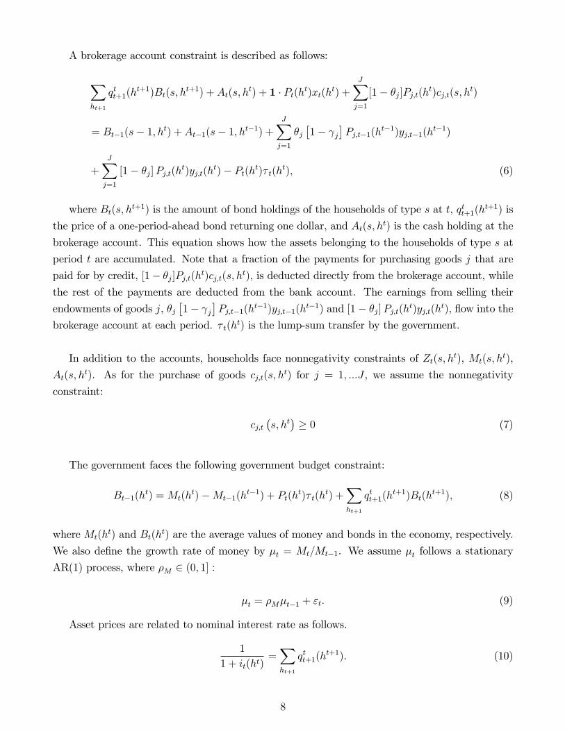
Figure 3 shows the IRFs of selected variables to a monetary policy shock. The line with black

diamonds depicts the equilibrium response of the price level of the numeraire, the line without

symbols displays that of the aggregate velocity of the economy, and the line with white circles

displays that of the aggregate money supply. We consider a one time, negative monetary policy

shock, by one unit, that happens at period 0. The �gure indicates a sluggish dynamics of the

numeraire price, relative to a money supply in a wake of monetary policy shock. The price level of

numeraire does not fall one-for-one with the drop of aggregate money supply. As a consequence,

an aggregate velocity, which is de�ned by (11) rises, in the short run.

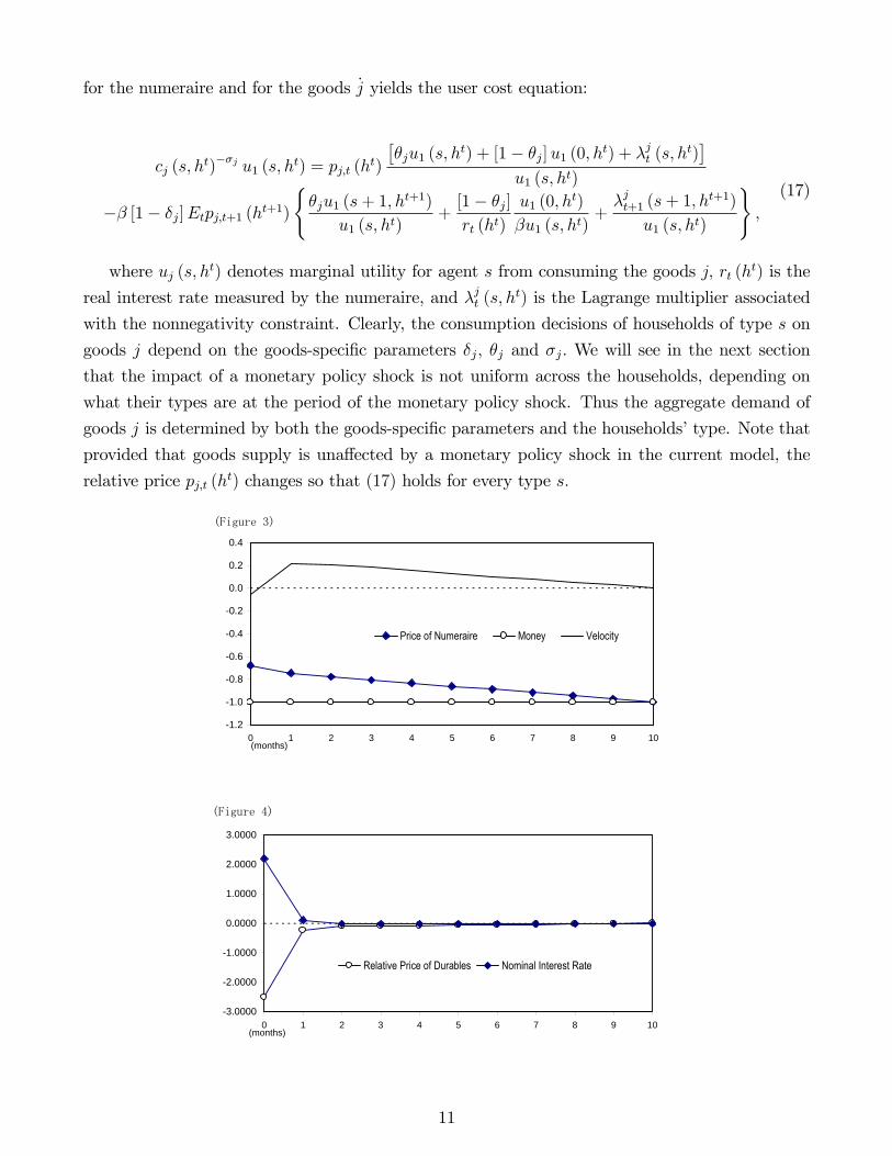
In Figure 4, the line with black diamonds displays the equilibrium response of the nominal

interest rate to the monetary policy shock, and the line with white circles displays that of the

relative price of durables. Upon the shock, as the quantity of money supply drops in the �nancial

market, the nominal interest rate rises (liquidity e¤ect. see, for example, Edmond and Weill

(2005)). As for the relative price of durables, the time path shows that it declines for a while and

returns to the steady state.

As discussed in Alvarez et al. (2003) and Edmond and Weill (2005), the inventoy-theoretic

model delivers the price sluggishness in an environment where the price is �exible. Price level

deviates from the quantity of money in the short run. In the next section, we argue that the model

also implies that the price responses of goods to a monetary policy shock are not uniform. Figure

4 indicates that the price response of durable is di¤erent from that of non-durable. We examine

the underlying mechanism that renders this heterogeneity of price responses in the section below.

3 Relative price responses and goods characteristics

In this section, we investigate the link between the characteristics of goods, and the price responses

of goods to a monetary policy shock. We claim that the characteristics of goods are the important

determinants of the observed price response dispersions across goods in a monetary policy shock.

A consumption theory, such as Bils and Klenow (1998), provides theoretical grounds for the

model implications. Because explicit production sectors are missing in our model, households�

consumption decisions are the only source of the dispersion of the price responses across goods

to a monetary policy. For a given income level, households�decisions about their expenditure

on goods are a¤ected by the characteristics of the goods. That is, durability, cash-intensity and

12

luxuriousness of the goods are playing a part in households�demand decisions. Bils and Klenow

(1998), using the representative agent model, show that following an increase in income, the

households�demands for durables and luxuries tend to be higher compared with the demand for

the �numeraire�.

Our model is not a representative agent model, and households are heterogeneous in terms of

the timing of the rebalancing of their assets. A monetary policy shock, in this environment, does

not bring a uniform increase of wealth to all the households. The size and the sign of the impact

of the monetary policy shock for households is type speci�c.

(Figure 5)

­0.50

­0.40

­0.30

­0.20

­0.10

0.00

0.10

0.20

14 13 12 11 10 9 8 7 6 5 4 3 2 1 0

ρ_m = 0.0 ρ_m = 0.2

ρ_m = 0.6

(two­year cumulative sum of  the response of numeraire cunsumption)

(type s ; a number of months it takes the households to rebalance the assets)

To see this quantitatively, we show how household type matters to the households�responses to

a monetary policy shock. Figure 5 plots the CIRs of the numeraire consumption for each household

after a monetary contraction shock, in terms of the deviation from the steady state. Along the

x-axis, each household is grouped according to its type at the period when the policy shock occurs.

For each household type of s = 0; :::14; a positive (negative) value of CIR along the y-axis indicates

the household increases (decreases) the numeraire consumption after the monetary policy shock,

implying the household becomes richer (poorer) upon the shock. The line with black diamonds

denotes the CIRs when the policy shock is one time, and one unit decline of money growth rate.

This corresponds to the case where �M = 0:0 (see, (9)): The line with white circles, and the line

without circles depict the CIRs of the numeraire consumption for the case where �M = 0:2 and for

the case where �M = 0:6, respectively.

Figure 5 shows, for all three speci�cations of �M ; that the CIRs of the numeraire consumptions

take negative values for households with smaller s at the period of innovation; and positive values

for households with larger s at the same period:While the persistency of the money growth shock

to some extent changes the pattern of the distribution, it is clear that the impact of the monetary

policy shock is di¤erent across the households, depending on the household type at the period of

innovation. For example, for households that are type s = 0 at the occurrence of the policy shock,

the monetary policy shock always works as a negative income shock that leads to the reduction

of the consumption. A fall in the money supply in the �nancial market results in the decline of

13

money holdings by the households who transfer money to their bank account at that time. The

portion of the real money balances held by these households shrink, and the households reduce

their goods purchases. For those that have rebalanced their assets before the policy shock, the

shock works as a positive income shock that results in an increases in their consumption. Their

money holdings are invariant to the shock, but the price level of goods become lower after the

shock as the aggregate money stock shrinks, and they become richer in the short run.

In this section, we see that the response of each household to an income shock is an important

determinant of household�s expenditure decision. It is notable, however, that the equilibrium

relative price response of goods j is determined by the relative size of the aggregate demand for the

goods j; compared with the aggregate demand for the numeraire, which re�ects the consumption

decisions of those heterogenous households discussed above.

3.1 Durables vs Non-durables

First, we examine the role of durability of goods in determining their price responses to a monetary

policy shock. To see this, we consider goods j with �j, which is strictly smaller than unity. We

assume that goods j is di¤erent from the numeraire only in terms of its durability. That is, �jand �j are both unity.

If we ignore the terms associated with the nonnegativity constraint for simplicity, combining

the �rst order conditions for the households of type s; with respect to goods j and the numeraire

yields the user cost equation:

uj (s; ht)

u1 (s; ht)= pj;t

�ht�� � [1� �j]Etpj;t+1

�ht+1

� u1 (s+ 1; ht+1)u1 (s; ht)

; (18)

where pj;t (ht) is the relative price of the goods j with respect to the numeraire, and uj (s; ht)

denotes the marginal utility of the service �ow from an additional unit of the durables j; for

households of type s:

According to Bils and Klenow (1998), consumption theory implies that the durables expenditure

cj (s; ht) is more responsive to an income change, than the non-durables expenditure c1 (s; ht) :

Suppose that there is an unexpected increase in households�income at t� 1; and that the relativeprice pj;t (ht) is constant, then the �rst order conditions derived from the utility function (2) gives

us the following relations:

~cj�s; ht

�=~kj (s; h

t)

�j> ~kj

�s; ht

�= ~c1

�s; ht

�; (19)

where ~xj (s; ht) is the percentage deviation of the variable xj (s; ht) ; around the non-stochastic

steady state. This equation says that in a wake of positive income shock, goods j is more needed

by the households than the numeraire, at period t: A lower depreciation rate implies that goods

j is more preferred by the households. If a shock of an equal size but opposite sign happens,

14

conversely, goods with lower depreciation rate is less wanted. In an economy where goods supply

is unchanged, the relative price pj;t (ht) varies, so as to clear the market.

As we have seen in Figure 5 above, a monetary policy shock, in our model, invokes a distri-

butional shock across household types. While aggregate quantities of goods are unaltered by the

monetary policy shock, some types of households reduce their consumption, while others increase

their consumption. In our economy, households hit by a positive income shock and those hit by a

negative income shock coexist.

(Figure 6)

­0.35

­0.30

­0.25

­0.20

­0.15

­0.10

­0.05

0.00

0.05

0.10

0.15

0 1 2 3 4 5 6 7 8 9 10 11 12 13 14 15

delta = 1 delta = 0.8

delta = 0.6 delta = 0.4

(months)

­4.0

­3.5

­3.0

­2.5

­2.0

­1.5

­1.0

­0.5

0.0

0.5

0.05 0.15 0.25 0.35 0.45 0.55 0.65 0.75 0.85 0.95

CIR (6 months) CIR (12 months)

CIR (24 months)

(delta)

­2.50

­2.00

­1.50

­1.00

­0.50

0.00

0.50

0 1 2 3 4 5 6 7 8 9 10

theta = 1 theta = 0.8

theta = 0.6 theta = 0.4

(months)

­4.5

­4.0

­3.5

­3.0

­2.5

­2.0

­1.5

­1.0

­0.5

0.0

0.00 0.10 0.20 0.30 0.40 0.50 0.60 0.70 0.80 0.90

CIR (6 months) CIR (12 months)

CIR (24 months)

(Theta)

­4.0

­3.5

­3.0

­2.5

­2.0

­1.5

­1.0

­0.5

0.0

0.5

0.05 0.15 0.25 0.35 0.45 0.55 0.65 0.75 0.85 0.95

CIR (6 months) CIR (12 months)

CIR (24 months)

(delta)

­4.5

­4.0

­3.5

­3.0

­2.5

­2.0

­1.5

­1.0

­0.5

0.0

0.00 0.10 0.20 0.30 0.40 0.50 0.60 0.70 0.80 0.90

CIR (6 months) CIR (12 months)

CIR (24 months)

(Theta)

The upper panel in Figure 6 displays IRFs of the relative price of durables j over the numeraire,

to a monetary policy innovation. We consider one time negative shock to money growth, by one

unit, as before (monetary contraction). The IRFs are drawn for the various annual depreciation

rates of goods j; �j: See Appendix A for details of other parameterizations.

The �gures show that the durables price drops in a monetary contraction, compared with the

numeraire�s price. When �j is unity, the relative price is una¤ected by the monetary policy shock.

As goods become more durable, prices decline more severely. This observation implies that the

fall in demand for goods j by the poor households outweighs the rise in demand for goods j by

rich households. The lower panel of Figure 6 reports the CIRs of the relative price of goods j; as a

function of the depreciation rate �j: For each �j; the CIRs are calculated for a 6-month period, a

15

12-month period and a 24-month period. For all the CIRs with di¤erent time horizons, the size of

the relative price decline measured by the CIRs, is larger for the goods with a smaller depreciation

rate �j.

The same pattern is observed even when we change the parameterization of the model. Table

C1 in Appendix C represents the CIRs of the relative price of goods j to a contractionary monetary

policy innovation, for several di¤erent rates of annual depreciation. We report the CIRs for several

parameterizations of money growth persistency parameter �M ; and the frequency with which the

households access to their brokerage accounts, N�1: We consider �M = 0:0; 0:2; 0:4; 0:6; and

0:8. For N; we consider N = 6; 15 and 24: For each combination of �M and N; a reduction

in depreciation rate �j leads to larger negativeness of the CIRs. Moreover, given the size of

depreciation rate, either higher �M or higher N implies larger negative CIRs for the relative price

of goods j:

3.2 Credit goods vs Cash goods

Second, we examine the importance of cash goods vs credit goods distinction, for the price responses

of the items to a monetary policy shock. Earlier works in monetary economics, such as Lucas and

Stokey (1987), Ogaki (1988), Hodrick et al. (1991) and Kakkar and Ogaki (2002), consider an

economy where certain types of goods are purchased only with cash, and other goods are purchased

only with privately o¤ered credit contracts.

For instance, Kakkar and Ogaki (2002) regard that non-durable consumption and food con-

sumptions as cash goods, and Ogaki (1988) regards automobiles as credit goods.

In Aizcorbe et al. (2003), the amount of debt of U.S. families is distributed by the purpose of

the debt, based on the Survey of Consumer Finances. They report that throughout the surveys

in 1992, 1995, 1998 and 2001, �Home purchase� and �Vehicles� constituted about 80% of the

total amount of debt of all families, while the shares of �Goods and service�and �Education�are

small. Klee (2008), using grocery store scanner data, shows that households�payment substitution

between cash, debit card, credit card and check is correlated with average value per item they

purchase. These empirical studies are consistent with the view that certain types of goods are

always credit goods, and others are always cash goods.

There are, however, other empirical studies that shed lights on the di¤erent aspect of the

payment system. Empirical studies by Borzekowski et al. (2006) �nd the cohort e¤ect in the con-

sumers�choice of payment instrument. That is, the payment instrument depends on the consumers�

ages. Klee (2008) also reports that choice of the payment is strongly related to demographics. This

suggests that payment instruments are rather agent speci�c, and distinctions such as cash goods

vs credit goods may be misleading. In this paper, however, we follow the presumption that cash

intensiveness and credit intensiveness is goods speci�c characteristics.

Consider a credit goods j whose �j is zero. �j = 0 indicates that the goods j is cash-goods. By

assumption, transaction of goods j are free from in�ationary tax. Assuming goods j only di¤ers

16

from the numeraire by �j; the �rst order conditions associated with the numeraire and goods j are

reduced to:

uj�s; ht

�= pj;t

�ht�u1�0; ht

�; (20)

where pj;t (ht) is the relative price of goods j over that of the numeraire. Using the resource

constraints (12), the deviation of the relative price of goods j is described by the following equation:

~pj;t�ht�= �~u1

�0; ht

��1= �~c1

�0; ht

�; (21)

where � is a positive constant. This equation says that the relative price of goods j, ~pj;t (ht),

increases one-for-one with the increase of ~u1 (0; ht)�1, or equivalently with ~c1 (0; ht) : Note that as

~pj;t (ht) re�ects the households�costs of paying a dollar from their brokerage accounts, instead of

from their bank accounts, the variations of the prices are associated with the variations of utility

of the households of type s = 0:When a monetary contraction induces a shortage of money supply

in the �nancial market, a cost of paying a dollar from the brokerage account measured by u1 (0; ht)

increases. A dollar in the brokerage account becomes more precious than a dollar in the bank

account, and households avoid purchasing goods that are linked to the reduction of a dollar from

the brokerage account. A monetary contraction leads to a decline in demand for credit goods j;

for all the types of households. The relative price ~pj;t (ht) then drops to clear the market.

(Figure 7)

­2.50

­2.00

­1.50

­1.00

­0.50

0.00

0.50

0 1 2 3 4 5 6 7 8 9 10

theta = 1 theta = 0.8

theta = 0.6 theta = 0.4

(months)

­4.5

­4.0

­3.5

­3.0

­2.5

­2.0

­1.5

­1.0

­0.5

0.0

0.00 0.10 0.20 0.30 0.40 0.50 0.60 0.70 0.80 0.90

CIR (6 months)CIR (12 months)CIR (24 months)

(Theta)

­0.0015

­0.0010

­0.0005

0.0000

0.0005

0.0010

0.0015

0.0020

0.0025

0 1 2 3 4 5 6 7 8 9 10 11 12 13 14 15

sigma = 1.2 sigma = 1.1

sigma = 1.0

(months)

­0.07

­0.06

­0.05

­0.04

­0.03

­0.02

­0.01

0.00

0.01

0.02

0.03

0.50 0.60 0.70 0.80 0.90 1.00 1.10 1.20 1.30 1.40

CIR (6 months)

CIR (12 months)

CIR (24 months)

(sigma)

17

­4.5

­4.0

­3.5

­3.0

­2.5

­2.0

­1.5

­1.0

­0.5

0.0

0.00 0.10 0.20 0.30 0.40 0.50 0.60 0.70 0.80 0.90

CIR (6 months) CIR (12 months)

CIR (24 months)

(Theta)

­0.07

­0.06

­0.05

­0.04

­0.03

­0.02

­0.01

0.00

0.01

0.02

0.03

0.50 0.60 0.70 0.80 0.90 1.00 1.10 1.20 1.30 1.40

CIR (6 months) CIR (12 months)

CIR (24 months)

(sigma)

The upper panel in Figure 7 displays IRFs of the relative price of credit goods j over the

numeraire goods, to a contractionary monetary policy shock for the various �j:We consider the

same monetary policy shock as in the previous section. Compared with the numeraire�s price, the

credit goods�price declines in a monetary contraction. As goods become less cash intensive, the

price declines are more severe.

The lower panel of Figure 7 reports the CIRs, as a function of the size of �j: For each �j; the

CIRs for 6-month period, 12-month period and 24-month period are plotted. For all CIRs with

di¤erent time horizons, the size of the relative price decline measured by the CIRs, is larger for

the goods with smaller �j.

The role of �j in determining the relative price responses to a monetary policy innovation is

unchanged in an economy where the environments are altered. Table C2 in Appendix C shows

the CIRs of the relative price of goods j to a contractionary monetary policy shocks, for several

di¤erent degrees of cash intensity. As before, we report the CIRs for several parameterizations of

�M ; and N: For each combination of �M and N; a reduction in cash intensity �j leads to larger

negativeness of the CIRs. Moreover, given the level of cash intensity, either a higher �M or a higher

N implies more negative CIRs of the relative price of goods j:

3.3 Luxuries vs Necessities

The third characteristic we consider is the distinction between luxuries and necessities. Following

Bils and Klenow (1998), the luxuriousness in our model is captured by the parameter �j in addilog

utility functions (2), where a higher �j corresponds to necessities. Consider a goods j with �j,

that only di¤ers from the numeraire by the income elasticity. That is, both �j and �j are unity.

In this speci�cation, the user cost equation for the goods j and the numeraire is expressed as:

uj�s; ht

�= pj;t

�ht�u1�s; ht

�; (22)

where pj;t (ht) is the relative price of the goods j with respect to the numeraire. Bils and Klenow

(1998) argue that assuming that the relative price change pj;t is unchanged, luxury is preferred to

18

the numeraire when the households receive an unexpected positive income shock. (22) with our

utility function (1) yields:

~cj;t�s; ht

�=1

�j~c1;t�s; ht

�: (23)

That is, given a change in consumption of the numeraire denoted by ~c1;t; the demand for goods

j increases by ~c1;t��1j : Note that �j > 0 indicates that goods j consumption ~cj;t (s; ht) and ~c1;t (s; ht)

co-move upon an income shock, and that �j a¤ects the relative size of ~cj;t (s; ht), with respect to

~c1;t (s; ht). Higher (lower) �j implies that goods j is less (more) demanded by the household of

type s; compared with the numeraire, in a wake of positive income shock. As we have discussed

above, in our speci�cation, pj;t (ht) clears the markets for both goods j and the numeraire at the

equilibrium.

Using the resource constraints (12), the deviation of the relative price of goods j is described

by the following equation:

~pj;t =

N�1Xs=0

�c1(s)1�j

!�1 N�1Xs=0

�c1(s)1�j ~c1;t(s): (24)

This equation indicates that the relative price of goods j, ~pj;t (ht), is determined by the linear

combination of ~c1;t(s; ht) for s = 0; :::; N � 1: If all agents in an economy reduce their expendituresin a monetary contraction, (23) indicates that the demands toward luxury lessen more, compared

with those toward the numeraire. Then the price of goods with lower �j should decline quicker

than the numeraire to clear the market. As we have seen in the previous sections, however,

the signs of the income shocks to each households are not the same. The size and the sign of

the relative price changes, ~pj;t(ht); after a monetary policy shock, are dependent on both how

each types of the households respond to the shock, and the relative signi�cance of the household,�PN�1s=0 �c1(s)

1�j

��1�c1(s)

1�j :

(Figure 8)

­0.0015

­0.0010

­0.0005

0.0000

0.0005

0.0010

0.0015

0.0020

0.0025

0 1 2 3 4 5 6 7 8 9 10 11 12 13 14 15

sigma = 1.2 sigma = 1.1

sigma = 1.0

(months)

­0.07

­0.06

­0.05

­0.04

­0.03

­0.02

­0.01

0.00

0.01

0.02

0.03

0.50 0.60 0.70 0.80 0.90 1.00 1.10 1.20 1.30 1.40

CIR (6 months) CIR (12 months)

CIR (24 months)

(sigma)

­0.0015

­0.0010

­0.0005

0.0000

0.0005

0.0010

0.0015

0.0020

0.0025

0 1 2 3 4 5 6 7 8 9 10 11 12 13 14 15

sigma = 1.2 sigma = 1.1

sigma = 1.0

(months)

­0.07

­0.06

­0.05

­0.04

­0.03

­0.02

­0.01

0.00

0.01

0.02

0.03

0.50 0.60 0.70 0.80 0.90 1.00 1.10 1.20 1.30 1.40

CIR (6 months) CIR (12 months)

CIR (24 months)

(sigma)

19

­0.07

­0.06

­0.05

­0.04

­0.03

­0.02

­0.01

0.00

0.01

0.02

0.03

0.50 0.60 0.70 0.80 0.90 1.00 1.10 1.20 1.30 1.40

CIR (6 months) CIR (12 months)

CIR (24 months)

(sigma)

­0.07

­0.06

­0.05

­0.04

­0.03

­0.02

­0.01

0.00

0.01

0.02

0.03

0.50 0.60 0.70 0.80 0.90 1.00 1.10 1.20 1.30 1.40

CIR (6 months) CIR (12 months)

CIR (24 months)

(sigma)

The upper panel in Figure 8 displays the IRFs of the relative price of goods j over the nu-

meraire, to a contractionary monetary policy shock for the various �j � 1:We consider the samemonetary policy shock as in the previous sections. Compared with the numeraire�s price, the price

of necessities rises in a monetary contraction. As goods becomes more luxurious, that is as �japproaches unity, the rise in the relative price gets smaller.

The lower panel of Figure 8 reports the CIRs of the relative price of goods j; as a function of

the income elasticity parameter �j: For each �j; the CIRs for 6-month period, 12-month period

and 24-month period are plotted. For all CIRs with di¤erent time horizons, the size of the relative

price decline, measured by the CIRs, is larger for the goods with smaller �j. If �j is smaller than

unity, the goods are luxurious, and the relative prices decline upon the shock. For goods with �jgreater than unity (necessity), the relative price rises, upon the same shock.

Similarly to the experiments conducted in the previous sections, we test the robustness of this

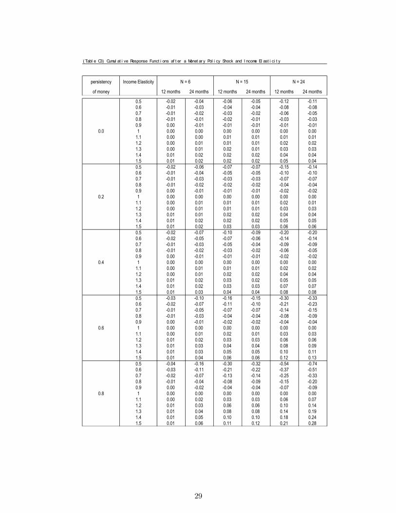
pattern, using various other parameterizations. Table C3 in Appendix C shows the CIRs of the

relative price of goods j; to contractionary monetary policy shocks, for several di¤erent values of

income elasticity parameter. As we did before, we report the CIRs for several parameterizations

for �M and N: For each combination of �M and N; a reduction in income elasticity parameter �jleads to larger negativeness in CIRs. Moreover, for a given size of �j, either a higher �M or a

higher N implies more negative CIRs for the relative price of goods j:

4 Empirical evaluation

In this section, we empirically investigate the link between the responses of relative prices to a

monetary policy shock and the goods�characteristics. We test our model using two econometric

procedures: a measure of the monetary policy innovation developed in Romer and Romer (2004),

and the factor-augmented VAR proposed in Bernanke et al. (2005). See Appendix B for details.

Mapping from the relative price responses of speci�c goods to a monetary policy shock to the

goods�characteristics requires rich knowledge about the goods�characteristics, such as the size of

�j; �j and �j of the goods. In the empirical analysis below, most of these goods-speci�c parameters

20

are taken from the previous studies, especially from Bils and Klenow (1998). They report two series

of goods-speci�c parameters, that are directly related to �j and �j. One series is �Expected life

of service time� reported for 43 consumption goods. These �gures are based on an intero¢ ce

memo of a major property-casualty insurance company and Fixed Reproducible Tangible Wealth

published by the Bureau of Economic Analysis. We calculate the depreciation rate �j of goods j

from the reported expected lives of goods j. For the items that belong to service in PCE, Bils

and Klenow (1998) do not provide the associated depreciation rates. We assume that all items

in Service have a unit depreciation rate. The other series that Bils and Klenow (1998) report is

related to the goods�speci�c income elasticity �j. Using the panel data released from the Bureau

of Labor Statistics, they estimate the goods-speci�c �Engel curves�for many consumption goods.

Their de�nition of the �Engel curve� is the elasticity of expenditure on goods j with respect to

households�total nondurable consumption. From (23) ;this elasticity of expenditure corresponds

to ��1j in our model. As Bils and Klenow (1998) concentrate their analysis on goods, we have

limited sample data for �j in which the items that belong to services are not included.

Lastly, we set the parameters for cash intensity of goods j, �j; based on the premise made in

Kakkar and Ogaki (2002). Following them, foods are regarded as cash goods whose �js are unity

in our empirical analysis. As we do not know the cash intensity for the other goods, we use dummy

variable for the PCE items that belong to food, and check whether those dummies are signi�cant

in the estimation.

To see the role of goods� characteristics in determining the price responses of goods j, we

follow Davis and Haltiwanger (2001) and Boivin et al. (2007). We �rst calculate impulse response

functions (IRFs) for a monetary policy shock, either using the regression developed in Romer and

Romer (2004) or using FAVAR, for each PCE item. We then regress the CIRs calculated for each

item, on the each item�s characteristic parameters, �j; �j and �j.

We run �ve regressions where the dependent variable is always the CIRs of the relative prices

for each goods, and the explanatory variables are each one of the goods characteristic paramters

discussed earlier: depreciation rate (LS1), income elasticity (LS2), food dummy (LS3), and fre-

quency of price adjustment (LS4). We also run a regression where all the depreciation rates,

income elasticities and food dummies are included as the explanatory variables (LS5). As the

parameters reported in Bils and Klenow (1998) are limited to goods, the samples used in LS2 and

LS5 include only durables and nondurable goods, while the samples used in LS1, LS3 and LS4include durables, nondurable goods and services (see Appendix B for details).

21

(Table 2)(regression of CIRs of relative prices on goods' characteristics, CIRs estimated by Romer and Romer (2004))

LS (1) LS (2) LS (3) LS (4) LS (5)(explanatory variable)

constant ­0.11* ­0.27* ­0.07* 0.01 ­0.29*(0.04) (0.13) (0.03) (0.04) (0.13)

δ 0.21* 0.39(0.05) (0.21)

σ 0.37* 0.20*(0.17) (0.17)

food dummy 0.08** ­0.16(0.06) (0.19)

freqnency 0.28(0.31)

Figures in brankets are standard deviation, that are calculated by bootstrap.* denotes 5% significance, and ** denotes 10% significance.

(Table 3)(regression of CIRs of relative prices on goods' characteristics, CIRs estimated by FAVAR)

LS (1) LS (2) LS (3) LS (4) LS (5)(explanatory variable)

constant ­0.28* ­0.51* ­0.03 0.13 ­0.67*(0.09) (0.25) (0.05) (0.06) (0.20)

δ 0.35* 0.50(0.11) (0.31)

σ 0.57* 0.30*(0.33) (0.21)

food dummy ­0.31 0.48*(0.11) (0.26)

freqnency ­0.78*(0.22)

Figures in brankets are standard deviation, that are calculated by bootstrap.* denotes 5% significance, and ** denotes 10% significance.

Table 2 reports the results where a measure of Romer and Romer (2004) is used for the

estimation. Table 3 reports the cases where the dependent variables (CIRs) are estimated by

FAVAR. For both cases, we consider a positive innovation in Federal Fund Rate as a contractionary

monetary policy shock.

As for the durability of goods �; it is noticeable from both Table 2 and Table 3, that the relative

price of items that have higher durability (or equivalently, lower �) tend to descend in monetary

contraction shock. Regressions in which goods and services are included in the samples (LS1 and

LS2) yield the positive and signi�cant coe¢ cients for depreciation rate of items. In the regressions

22

where items in services are excluded from the sample (LS5), the coe¢ cients become less signi�cant

(11% signi�cance), but the estimated sign for � is consistent with the model.

As for the income elasticity of goods �; it is also evident that the relative price of items that have

higher income elasticity (or equivalently, smaller �) tend to descend in a monetary contraction.

The sign and the signi�cance of � are maintained in both speci�cations of the estimations (LS2and LS5).

The role of the food dummy is, on the other hand, not clear from the data. The coe¢ cient

estimated by the Romer and Romer measure has the correct sign and is signi�cant, but the

coe¢ cient estimated using FAVAR has the opposite sign. Weakness in the regressions relating

the CIRs of the prices and the cash intensities lies on the fact that we do not have explicit goods

speci�c �gures for cash intensity. In addition, as we discussed above, the assumption that some

goods are always purchased with cash and the others are purchased with credit may be a strong

assumption.

The quantitative role of the frequency of price adjustments in determining the relative price

responses of goods is also ambiguous. Along the line of the standard Keynesian model, including

Carvalho (2006), higher frequency of price adjustment suggests more negativeness in the rela-

tive price responses of goods to a contractionary monetary shock. This theoretical prediction is

consistent with the FAVAR estimates, but it is not so with the results by Romer and Romer (2004).

In summary, our empirical result suggests that there is a model implied relationship between

the estimated relative price responses of PCE items, and the goods�characteristics parameters

reported in Bils and Klenow (1998) and Kakkar and Ogaki (2002). That is, the relative prices of

more durable goods and more luxurious goods tend to descend in a wake of monetary contraction.

The role of cash intensity in determining the price responses of goods to a monetary policy shock

is less apparent from our experiments.

5 Conclusion

In this paper, we provided a theoretical basis for understanding the price responses of goods

to a monetary policy shock. Using an inventory-theoretic model of money demand framework,

we show that the characteristics of the consumption goods are important determinants of the

price dynamics of goods after a monetary policy shock. Our model implies that prices of more

durable goods, more luxurious goods and less cash intensive goods descend more to a monetary

contraction shock, compared with the price of the numeraire. This implication is robust to the

various parameterizations of the model, such as the persistency of the money growth rate, and the

frequency of asset rebalancing for households.

We estimate the relative price responses of goods to a monetary policy shock, using the mon-

etary policy shock measure provided in Romer and Romer (2004), and FAVAR developed in

Bernanke et al (2005). We examine whether the estimates of those relative prices are statisti-

23

cally related to the goods speci�c parameters of durability, luxuriousness and the cash intensity

of goods that are reported in Bils and Klenow (1998) and Ogaki and Kakkar (2002). In terms

of durability and luxuriousness, both Romer and Romer (2004) and FAVAR yield the pattern of

relative price responses that are consistent with our model. We, however, do not �nd an empirical

evidence that relative prices of credit goods fall following a monetary policy shock. One interpre-

tation of this observation may be that the payment instruments are rather agent speci�c, and not

goods speci�c.

Appendix A: Parameters for calibration

In Section 2.3, we simulate our model using a two-sector speci�cation. A two-sector model where an

economy is composed of a non-durables sector and a durables sector is analyzed in the previous literature,

such as Erceg and Levin (2006) and Barsky et al. (2007). The non-durable sector is numbered as one,

and the durables sector is numbered as two. The simulation is conducted monthly. The parameters used

for the simulations are;

Parameters

Parameter Value Description

N 15 Period of the cycle

� 0.962 Discount factor

�1 1.00 Intertemporal elasticity of substitution of numeraire

�2 1.00 Intertemporal elasticity of substitution of durables

� 0.2 Durable share parameter

� .22 Depreciation of durables

1 0.6 Ratio endowed to banking account

2 0.6 Ratio endowed to banking account

� 1.05 Mean of money growth

�� 0.00 Persistence of money growth shock

�� 1 s.d. of money growth innovation

The parameters, N; �1; �2; 1; 2; ��; ��; �� are taken from Alvarez et al. (2003). � corresponds to the

steady state share of the durables goods, and is set to be the long-run average nominal expenditure share

of durable (relative to total consumption), which is around 0:2 in the US. For the annual depreciation

rate, we follow the speci�cation of Baxter (1996).

Appendix B: Description of the data

Price seriesThe disaggregated price data used in the current paper are the monthly series of personal consumption

expenditures (price indexes and nominal expenditure). Data are seasonally adjusted. All item series are

24

normalized by the price index of the aggregate non-durables, which we constructed from the nondurable

goods series and the services series of PCE, using a Tornqvist approximation (see Welan (2000)).

In each regression above, we drop some of the items for the following reasons.

In estimating the regressions where the frequencies of price adjustments of goods are involved, we

disregard some of the samples because of the di¢ culties of relating the price indices of the PCE items to

their frequencies, reported in Nakamura and Steinsson (2007). Among the PCE items in 2003, although

most of the items are de�ated by the consumer price indices (CPI), some items are de�ated by the

producer price indices (PPI) (e.g., proprietary hospitals) or other price measure (e.g., clubs & fraternal

organizations). In addition, there are items that are de�ated by the CPI but by broader categories of

the CPI than the item stratum (e.g., casino gambling). We exclude the items of the PCE that are not

de�ated by the CPI, and the items that are de�ated by broader categories than Major Group, CPI. These

procedures reduce the number of sample items that are for our regressions to 134.

Table 2 and Table 3 report regression of the CIRs on the depreciation rates. Our depreciation series

is based on Bils and Klenow (1998). Because of the lack of correspondence, we drop 12 items from the

134 items. For the same reason, the number of the sample in LS2 and LS5 is limited to 39.

Frequency of price adjustmentFigures for the frequency of price adjustment are taken from Nakamura and Steinsson (2007). All

the estimates reported in our paper refer to the frequency of price change by category for 1998-2005 in

Nakamura and Steinsson (2007). These series include sales. Their frequency data are constructed for

Entry Level Item (ELI) category, while each item�s stratum in PCE covers one or more ELIs. We average

the reported frequencies for each ELI with its weight reported in Nakamura and Steinsson (2007), to yield

frequencies of the CPI item stratum. The matching between ELI and CPI item stratum is done, using

the BLS Handbook of Methods, released by the Bureau of Labor Statistics.

Sample periodThe data sample period for the all estimations in the current paper is from January 1976 to December

1996. The initial period of the samples used in Boivin et al (2007) is January 1976, and the measure of

Romer and Romer (2004) is available from January 1969 to December 1996. The length of our sample

period is thus chosen so that the samples of the disaggregated price series are the same for both estimations,

FAVAR and the estimation using the measure of Romer and Romer (2004).

Calculating IRFs of disaggregated relative prices using Romer and Romer (2004)The IRFs of relative prices are estimated using the two measures of monetary policy innovations

mentioned above. In estimating the IRFs using the measure of monetary policy shocks developed by

Romer and Romer (2004), we use the following regression for each of the relative prices, based on Romer

25

and Romer (2004):

�pj;t (j) = c0 +24Xi=1

�i�pj;t�i (j) +

48Xi=1

ci�St�i + et; (25)

where �pj;t (j) is the log-di¤erence of each of the disaggregated relative price index of goods j, and

c0; �i and ci are the estimated parameters of the explanatory variables. St is the monetary policy shock

provided in Romer and Romer (2004).

Calculating IRFs of disaggregated relative prices using FAVARIn estimating the IRFs using the FAVAR methodology, we need to specify a panel of economic indi-

cators, to estimate common factors. In Bernanke et al. (2005), the panel contains 120 macroeconomic

variables. In addition to the variables employed in Bernanke et al. (2005), we add 194 real personal

consumption expenditure series, 154 producer price indices and 194 relative price series of personal con-

sumption expenditure series. They are transformed to the stationary series by taking the �rst di¤erence

of their logarithms.

26

5.1 Appendix C: Robustness tests

(Table C1) Cumulative Response Functions after a Monetary Policy Shock and Depreciation Rate

persistency depreciation rate N = 6 N = 15 N = 24

of money 12 months 24 months 12 months 24 months 12 months 24 months

0.1 ­1.54 ­1.55 ­3.30 ­3.24 ­4.73 ­4.570.2 ­1.51 ­1.51 ­3.17 ­3.10 ­4.50 ­4.350.3 ­1.49 ­1.50 ­2.48 ­2.41 ­2.09 ­2.060.4 ­1.49 ­1.49 ­1.32 ­1.26 ­1.12 ­1.07

0.0 0.5 ­0.69 ­0.70 ­0.80 ­0.72 ­0.94 ­0.890.6 ­0.41 ­0.41 ­0.71 ­0.61 ­0.77 ­0.730.7 ­0.19 ­0.19 ­0.61 ­0.51 ­0.63 ­0.580.8 ­0.20 ­0.21 ­0.49 ­0.42 ­0.55 ­0.520.9 ­0.03 ­0.03 ­0.37 ­0.32 ­0.44 ­0.421.0 0.00 0.00 0.00 0.00 0.00 0.000.1 ­2.01 ­2.02 ­4.23 ­4.14 ­5.98 ­5.830.2 ­1.97 ­1.97 ­4.06 ­3.97 ­5.69 ­5.550.3 ­1.95 ­1.96 ­3.17 ­3.08 ­2.67 ­2.670.4 ­1.94 ­1.95 ­1.72 ­1.65 ­1.46 ­1.43

0.2 0.5 ­0.92 ­0.92 ­1.07 ­0.97 ­1.24 ­1.220.6 ­0.56 ­0.57 ­0.96 ­0.84 ­1.03 ­1.030.7 ­0.28 ­0.28 ­0.84 ­0.72 ­0.86 ­0.840.8 ­0.30 ­0.30 ­0.68 ­0.59 ­0.75 ­0.750.9 ­0.05 ­0.06 ­0.52 ­0.45 ­0.60 ­0.621.0 0.00 0.00 0.00 0.00 0.00 0.000.1 ­2.84 ­2.85 ­5.85 ­5.72 ­8.14 ­8.010.2 ­2.79 ­2.80 ­5.62 ­5.50 ­7.75 ­7.640.3 ­2.77 ­2.77 ­4.38 ­4.26 ­3.69 ­3.760.4 ­2.76 ­2.76 ­2.45 ­2.34 ­2.09 ­2.12

0.4 0.5 ­1.33 ­1.33 ­1.57 ­1.44 ­1.79 ­1.860.6 ­0.84 ­0.84 ­1.42 ­1.27 ­1.52 ­1.590.7 ­0.43 ­0.43 ­1.24 ­1.10 ­1.27 ­1.330.8 ­0.47 ­0.47 ­1.03 ­0.91 ­1.11 ­1.180.9 ­0.11 ­0.11 ­0.78 ­0.69 ­0.87 ­0.961.0 0.00 0.00 0.00 0.00 0.00 0.000.1 ­4.62 ­4.64 ­9.30 ­9.15 ­12.62 ­12.710.2 ­4.55 ­4.57 ­8.97 ­8.82 ­12.04 ­12.130.3 ­4.52 ­4.54 ­6.96 ­6.82 ­5.87 ­6.220.4 ­4.51 ­4.52 ­4.08 ­3.92 ­3.49 ­3.75

0.6 0.5 ­2.20 ­2.20 ­2.69 ­2.50 ­3.04 ­3.380.6 ­1.41 ­1.41 ­2.44 ­2.24 ­2.60 ­2.940.7 ­0.75 ­0.74 ­2.13 ­1.95 ­2.16 ­2.450.8 ­0.83 ­0.83 ­1.75 ­1.62 ­1.86 ­2.170.9 ­0.26 ­0.26 ­1.33 ­1.22 ­1.46 ­1.751.0 0.00 0.00 0.00 0.00 0.00 0.000.1 ­9.71 ­10.38 ­19.69 ­21.00 ­25.80 ­28.710.2 ­9.61 ­10.28 ­19.09 ­20.36 ­24.70 ­27.520.3 ­9.57 ­10.24 ­15.15 ­15.78 ­13.11 ­15.180.4 ­9.55 ­10.22 ­9.39 ­9.61 ­8.29 ­9.92

0.8 0.5 ­4.97 ­5.12 ­6.31 ­6.41 ­7.27 ­9.060.6 ­3.34 ­3.45 ­5.71 ­5.85 ­6.19 ­7.930.7 ­2.00 ­2.08 ­4.97 ­5.15 ­5.09 ­6.620.8 ­2.15 ­2.26 ­4.11 ­4.31 ­4.34 ­5.800.9 ­1.03 ­1.10 ­3.12 ­3.30 ­3.36 ­4.651.0 0.00 0.00 0.00 0.00 0.00 0.00

27

( Tabl e  C2)   Cumul at i ve  Response  Funct i ons  af t er   a  Monet ar y  Pol i cy  Shock  and  Cash  I nt ensi t y

persistency cash intensity N = 6 N = 15 N = 24

of money 12 months 24 months 12 months 24 months 12 months 24 months

0.0 ­1.77 ­1.77 ­4.15 ­4.08 ­6.24 ­6.020.1 ­1.62 ­1.63 ­3.81 ­3.74 ­5.70 ­5.510.2 ­1.47 ­1.47 ­3.42 ­3.36 ­5.11 ­4.940.3 ­1.30 ­1.30 ­3.01 ­2.96 ­4.48 ­4.330.4 ­1.12 ­1.12 ­2.58 ­2.54 ­3.83 ­3.70

0.0 0.5 ­0.93 ­0.93 ­2.14 ­2.10 ­3.16 ­3.050.6 ­0.74 ­0.74 ­1.69 ­1.67 ­2.49 ­2.410.7 ­0.55 ­0.55 ­1.25 ­1.23 ­1.83 ­1.770.8 ­0.36 ­0.36 ­0.82 ­0.80 ­1.19 ­1.150.9 ­0.18 ­0.18 ­0.40 ­0.39 ­0.58 ­0.561 0.00 0.00 0.00 0.00 0.00 0.00

0.0 ­2.28 ­2.29 ­5.29 ­5.19 ­7.87 ­7.650.1 ­2.10 ­2.10 ­4.85 ­4.76 ­7.20 ­6.990.2 ­1.89 ­1.90 ­4.36 ­4.28 ­6.45 ­6.270.3 ­1.67 ­1.67 ­3.84 ­3.77 ­5.66 ­5.490.4 ­1.44 ­1.44 ­3.29 ­3.23 ­4.83 ­4.69

0.2 0.5 ­1.20 ­1.20 ­2.72 ­2.68 ­3.99 ­3.870.6 ­0.95 ­0.95 ­2.16 ­2.12 ­3.14 ­3.050.7 ­0.71 ­0.71 ­1.59 ­1.57 ­2.31 ­2.250.8 ­0.46 ­0.46 ­1.04 ­1.02 ­1.51 ­1.470.9 ­0.23 ­0.23 ­0.51 ­0.50 ­0.73 ­0.711 0.00 0.00 0.00 0.00 0.00 0.00

0.0 ­3.18 ­3.18 ­7.27 ­7.12 ­10.66 ­10.460.1 ­2.91 ­2.92 ­6.66 ­6.52 ­9.74 ­9.560.2 ­2.63 ­2.63 ­5.98 ­5.87 ­8.73 ­8.560.3 ­2.32 ­2.32 ­5.26 ­5.16 ­7.65 ­7.500.4 ­1.99 ­2.00 ­4.51 ­4.42 ­6.53 ­6.41

0.4 0.5 ­1.66 ­1.66 ­3.73 ­3.66 ­5.39 ­5.290.6 ­1.32 ­1.32 ­2.95 ­2.90 ­4.25 ­4.170.7 ­0.98 ­0.98 ­2.18 ­2.14 ­3.13 ­3.070.8 ­0.64 ­0.65 ­1.43 ­1.40 ­2.04 ­2.000.9 ­0.32 ­0.32 ­0.70 ­0.69 ­0.99 ­0.981 0.00 0.00 0.00 0.00 0.00 0.00

0.0 ­5.06 ­5.07 ­11.42 ­11.23 ­16.40 ­16.430.1 ­4.62 ­4.64 ­10.44 ­10.27 ­14.97 ­14.980.2 ­4.15 ­4.17 ­9.37 ­9.23 ­13.41 ­13.420.3 ­3.66 ­3.67 ­8.24 ­8.11 ­11.76 ­11.750.4 ­3.14 ­3.15 ­7.05 ­6.95 ­10.04 ­10.03

0.6 0.5 ­2.62 ­2.62 ­5.84 ­5.76 ­8.29 ­8.280.6 ­2.08 ­2.09 ­4.63 ­4.56 ­6.54 ­6.530.7 ­1.55 ­1.55 ­3.42 ­3.37 ­4.81 ­4.810.8 ­1.02 ­1.02 ­2.24 ­2.21 ­3.14 ­3.130.9 ­0.50 ­0.50 ­1.10 ­1.08 ­1.53 ­1.531 0.00 0.00 0.00 0.00 0.00 0.00

0.0 ­10.28 ­10.98 ­23.41 ­24.88 ­32.77 ­36.150.1 ­9.34 ­9.98 ­21.33 ­22.67 ­29.87 ­32.900.2 ­8.36 ­8.92 ­19.11 ­20.30 ­26.73 ­29.390.3 ­7.34 ­7.83 ­16.77 ­17.81 ­23.41 ­25.710.4 ­6.30 ­6.72 ­14.35 ­15.24 ­19.98 ­21.93

0.8 0.5 ­5.24 ­5.59 ­11.89 ­12.63 ­16.50 ­18.090.6 ­4.17 ­4.45 ­9.42 ­10.01 ­13.03 ­14.270.7 ­3.11 ­3.32 ­6.98 ­7.41 ­9.61 ­10.520.8 ­2.05 ­2.19 ­4.58 ­4.86 ­6.28 ­6.870.9 ­1.02 ­1.09 ­2.25 ­2.39 ­3.07 ­3.351 0.00 0.00 0.00 0.00 0.00 0.00

28

( Tabl e  C3)   Cumul at i ve  Response  Funct i ons  af t er   a  Monet ar y  Pol i cy  Shock  and  I ncome  El ast i ci t y

persistency Income Elasticity N = 6 N = 15 N = 24

of money 12 months 24 months 12 months 24 months 12 months 24 months

0.5 ­0.02 ­0.04 ­0.06 ­0.05 ­0.12 ­0.110.6 ­0.01 ­0.03 ­0.04 ­0.04 ­0.08 ­0.080.7 ­0.01 ­0.02 ­0.03 ­0.02 ­0.06 ­0.050.8 ­0.01 ­0.01 ­0.02 ­0.01 ­0.03 ­0.030.9 0.00 ­0.01 ­0.01 ­0.01 ­0.01 ­0.01

0.0 1 0.00 0.00 0.00 0.00 0.00 0.001.1 0.00 0.00 0.01 0.01 0.01 0.011.2 0.00 0.01 0.01 0.01 0.02 0.021.3 0.00 0.01 0.02 0.01 0.03 0.031.4 0.01 0.02 0.02 0.02 0.04 0.041.5 0.01 0.02 0.02 0.02 0.05 0.040.5 ­0.02 ­0.06 ­0.07 ­0.07 ­0.15 ­0.140.6 ­0.01 ­0.04 ­0.05 ­0.05 ­0.10 ­0.100.7 ­0.01 ­0.03 ­0.03 ­0.03 ­0.07 ­0.070.8 ­0.01 ­0.02 ­0.02 ­0.02 ­0.04 ­0.040.9 0.00 ­0.01 ­0.01 ­0.01 ­0.02 ­0.02

0.2 1 0.00 0.00 0.00 0.00 0.00 0.001.1 0.00 0.01 0.01 0.01 0.02 0.011.2 0.00 0.01 0.01 0.01 0.03 0.031.3 0.01 0.01 0.02 0.02 0.04 0.041.4 0.01 0.02 0.02 0.02 0.05 0.051.5 0.01 0.02 0.03 0.03 0.06 0.060.5 ­0.02 ­0.07 ­0.10 ­0.09 ­0.20 ­0.200.6 ­0.02 ­0.05 ­0.07 ­0.06 ­0.14 ­0.140.7 ­0.01 ­0.03 ­0.05 ­0.04 ­0.09 ­0.090.8 ­0.01 ­0.02 ­0.03 ­0.02 ­0.06 ­0.050.9 0.00 ­0.01 ­0.01 ­0.01 ­0.02 ­0.02

0.4 1 0.00 0.00 0.00 0.00 0.00 0.001.1 0.00 0.01 0.01 0.01 0.02 0.021.2 0.00 0.01 0.02 0.02 0.04 0.041.3 0.01 0.02 0.03 0.02 0.05 0.051.4 0.01 0.02 0.03 0.03 0.07 0.071.5 0.01 0.03 0.04 0.04 0.08 0.080.5 ­0.03 ­0.10 ­0.16 ­0.15 ­0.30 ­0.330.6 ­0.02 ­0.07 ­0.11 ­0.10 ­0.21 ­0.230.7 ­0.01 ­0.05 ­0.07 ­0.07 ­0.14 ­0.150.8 ­0.01 ­0.03 ­0.04 ­0.04 ­0.08 ­0.090.9 0.00 ­0.01 ­0.02 ­0.02 ­0.04 ­0.04

0.6 1 0.00 0.00 0.00 0.00 0.00 0.001.1 0.00 0.01 0.02 0.01 0.03 0.031.2 0.01 0.02 0.03 0.03 0.06 0.061.3 0.01 0.03 0.04 0.04 0.08 0.091.4 0.01 0.03 0.05 0.05 0.10 0.111.5 0.01 0.04 0.06 0.06 0.12 0.130.5 ­0.04 ­0.16 ­0.30 ­0.32 ­0.54 ­0.740.6 ­0.03 ­0.11 ­0.21 ­0.22 ­0.37 ­0.510.7 ­0.02 ­0.07 ­0.13 ­0.14 ­0.25 ­0.330.8 ­0.01 ­0.04 ­0.08 ­0.09 ­0.15 ­0.200.9 0.00 ­0.02 ­0.04 ­0.04 ­0.07 ­0.09

0.8 1 0.00 0.00 0.00 0.00 0.00 0.001.1 0.00 0.02 0.03 0.03 0.06 0.071.2 0.01 0.03 0.06 0.06 0.10 0.141.3 0.01 0.04 0.08 0.08 0.14 0.191.4 0.01 0.05 0.10 0.10 0.18 0.241.5 0.01 0.06 0.11 0.12 0.21 0.28

29

References

[1] Aizcorbe, A. M., A. B. Kennickell, B. M. Kevin B. Moore (2003) �Recent Changes in U.S.

Family Finances: Evidence from the 1998 and 2001 Survey of Consumer Finances,�Federal

Reserve Bulletin.

[2] Alvarez, F., A. Andrew, C. Edmond (2003) �On the Sluggish Response of Prices to Money in

an Inventory-Theoretic Model of Money Demand,�NBER working paper, 10016.

[3] Barsky, R. B., C. L. House, and M. S. Kimball (2007) �Sticky-Price Models and Durable

Goods,�American Economic Review, Vol. 97, No. 3.

[4] Baumol, W. J. (1952) �The Transactions Demand for Cash: An Inventory Theoretic Ap-

proach,�Quarterly Journal of Economics, Vol. 66, No. 4.

[5] Baxter, M. (1996) �Are Consumer Durables Important for Business Cycles?�Review of Eco-

nomics and Statistics, Vol. 78, No. 1.

[6] Bernanke, B. S., J. Boivin, P. Eliasz (2005) �Measuring the E¤ects of Monetary Policy: A

Factor-Augmented Vector Autoregressive (FAVAR) Approach,� Quarterly Journal of Eco-

nomics, Vol. 120, No. 1.

[7] Bils, M., P. J. Klenow (1998) �Using Consumer Theory to Test Competing Business Cycle

Models,�Journal of Political Economy, Vol. 106, No. 2.

[8] Bils, M., P. J. Klenow (2004) �Some Evidence on the Importance of Sticky Prices,�Journal

of Political Economy, Vol. 112, No. 5.

[9] Bils, M., P. J. Klenow, O. Kryvtsov (2003) �Sticky Prices and Monetary Policy Shocks�

Federal Reserve Bank of Minneapolis Quarterly Review, Vol. 27, No. 1.

[10] Boivin, J., M. Giannoni, and I. Mihov (2007) �Sticky Prices and Monetary Policy: Evidence

from Disaggregated US Data,�NBER working paper, 12824.

[11] Borzekowski, R. and E. K. Kiser (2006) �The Choice at the Checkout: Quantifying Demand

Across Payment Instruments,�Finance and Economics Discussion Series, Divisions of Re-

search & Statistics and Monetary A¤airs, Federal Reserve Board, April.

[12] Carvalho, C. (2006) �Heterogeneity in Price Stickiness and the Real E¤ects of Monetary

Shocks,�Frontiers of Macroeconomics, Vol. 2, No. 1.

[13] Chiu, J. (2005) �Endogenous Segmented Asset Market in an Inventory Theoretic Model of

Money Demand,�mimeo.

30

[14] Christiano, L. J., M. Eichenbaum, C. L. Evans (1999) �Monetary policy shocks: What have

we learned and to what end?,�Handbook of Macroeconomics, in: J. B. Taylor & M. Woodford

(ed.), Handbook of Macroeconomics, edition 1, Vol. 1, chapter 2.

[15] Davis, S. J. and J. B. Haltiwanger (2001) �Sectoral job creation and destruction responses to

oil price changes,�Journal of Monetary Economics, Vol. 48, No. 3.

[16] Edmond, C. and P. O. Weill (2005) �Models of the liquidity e¤ect� forthcoming in �The

New Palgrave Dictionary of Economics 2nd edition,�edited by S.N. Durlauf and L.E. Blume.

Palgrave Macmillan.

[17] Erceg, C. and A. Levin (2002) �Optimal Monetary Policy with Durable Consumption Goods,�

International Finance Discussion Paper, No.748, Board of Governors of the Federal Reserve

System.

[18] Erceg, C. and A. Levin (2006) �Optimal Monetary Policy with Durable Consumption Goods,�

Journal of Monetary Economics, Vol. 53, No. 7.

[19] Goodfriend M., R. G. King (1998) �The new neoclassical synthesis and the role of monetary

policy,�Working Paper 98-05, Federal Reserve Bank of Richmond.

[20] Grossman, S. and L.Weiss (1983) �A Transactions-BasedModel of the Monetary Transmission

Mechanism,�American Economic Review, Vol. 73, No. 5.

[21] Hayashi, F. (1985) �The Permanent Income Hypothesis and Consumption Durability: Analy-

sis Based on Japanese Panel Data,�Quarterly Journal of Economics, Vol. 100, No. 4.

[22] Hodrick, R. J., N. Kocherlakota, and D. Lucas (1991) �The Variability of Velocity in Cash-

in-Advance Models,�Journal of Political Economy, Vol. 99, No. 2.

[23] Kakkar, V. and M. Ogaki (2002) �The Distortionary E¤ects of In�ation: An Empirical Inves-

tigation,�mimeo.

[24] Khan, A. and J. K. Thomas (2007) �In�ation and Interest Rates with Endogenous Market

Segmentation,�Federal Reserve Bank of Philadelphia Working Paper 07-1.

[25] Khan, A., R. G. King, and A. L. Wolman (2003) : �Optimal Monetary Policy,�Review of

Economic Studies, Vol. 70, No. 4.

[26] Klee, E (2008) �How People Pay: Evidence from Grocery Store Data,�Journal of Monetary

Economics, Vol. 70, No. 4.

[27] Lucas, R. E., Jr. and N. L. Stokey (1987) �Money and Interest in a Cash-in-Advance Econ-

omy,�Econometrica, Vol. 55, No. 3.

31

[28] Mankiw, N. G. (1985) �Consumer Durables and the Real Interest Rate,�Review of Economics

and Statistics, Vol. 67, No. 3.

[29] Nakamura, Emi and J. Steinsson (2007) �Five Facts About Prices: A Reevaluation of Menu

Cost Models,�mimeo.

[30] Ohanian, L. E., A. C. Stockman, and L. Kilian (1995) �The E¤ects of Real and Monetary

Shocks in a Business Cycle Model with Some Sticky Prices,�Journal of Money, Credit, and

Banking, Part 2, Vol. 27, No. 4.

[31] Ogaki, M. (1988) �Learning about Preferences from Time Trends.�Unpublished Ph.D. dis-

sertation, University of Chicago, Chicago. Distortionary E¤ects of In�ation: An Empirical

Investigation,�mimeo.

[32] Romer, C. D. and D. H. Romer (2004) �New Measure of Monetary Shocks: Derivation and

Implications,�American Economic Review, Vol. 94, No. 4.

[33] Rotemberg, Julio and Michael Woodford (1997) �An Optimization-Based Econometric Frame-

work for the Evaluation of Monetary Policy,�NBER Macroeconomics Annual 1997.

[34] Tobin, J. (1956) �The Interest-Elasticity of Transactions Demand For Cash,�Review of Eco-

nomics and Statistics, Vol. 38, No. 3.

[35] Whelan, K. (2000) �A Guide to the Use of Chain Aggregated NIPA,�Finance and Economics

Discussion Series 2000-35, Board of Governors of the Federal Reserve System (U.S.).

32