introduction x a

BAIRE RESULTS OF MULTISEQUENCES

ROBERT TICHY AND MARTIN ZEINER

Dedicated to the memory of Edmund Hlawka

Abstract. We extend Baire results about nα-sequences in different ways, in

particular we investigate sequences with multidimensional indices.

1. Introduction

A sequence x = (xn)n∈N of real numbers is called uniformly distributed modulo 1,if for every pair a, b of real numbers with 0 ≤ a < b ≤ 1 the following conditionholds:

limn→∞

A([a, b), n,x)n

= b− a,

where A(I, n,x) is the number of elements xi, i ≤ n with xi ∈ I for an interval I.For a general theory of uniform distribution we refer to Kuipers and Niederreiter [11]and Drmota and Tichy [4].

In [7] Goldstern, Schmeling and Winkler studied the size (in the sense of Baire)of the set

U := {α ∈ R/Z : nα is uniformly distributed mod 1}for a given sequence n = (nj)j∈N of natural numbers; the size of this set dependson the growth rate of the sequence n. In particular they showed that U is meagerif n grows exponentially (for theory about Baire categories see Oxtoby [15]). ByAjtai, Havas, Komlos [2] this condition cannot be weakened.

Moreover it was proven in [7] that the set

V := {α ∈ R/Z : nα is maldistributed}is residual if n grows very fast (for the precise statement we refer to [7]).

The aim of this paper is to generalise these results in different ways. In Section 2we consider for a given sequence (nj)j∈N of r-dimensional vectors of nonnegativeintegers and an r-dimensional vector α of real numbers the sequence (njα)j∈N,where njα means the scalar product of two vectors. Afterwards we investigate inSection 3 in uniform distribution in Rd, i.e. for a d-dimensional sequence (nj) anda d-dimensional vector α we consider the sequence (njα)j∈N, where njα means theHadamard product of two vectors.

Section 4 is devoted to the generalisation of elementary properties of uniformdistribution of sequences to uniform distribution of nets. Afterwards we extendin Section 5 the characterisation of the set of limit measures of a sequence (see

Date: July 30, 2009.

2000 Mathematics Subject Classification. Primary: 11K38; Secondary: 11K06, 54E52.Key words and phrases. Baire category, nα-sequences, uniform distribution mod 1, nets, se-

quences with multidimensional indices.M. Zeiner was supported by the NAWI-Graz project and the Austrian Science Fund project

S9611 of the National Research Network S9600 Analytic Combinatorics and Probabilistic NumberTheory.

R. Tichy was supported by the Austrian Science Fund project S9611 of the National ResearchNetwork S9600 Analytic Combinatorics and Probabilistic Number Theory.

1

2 ROBERT TICHY AND MARTIN ZEINER

Winkler [18]) to a special kind of nets over Nd. Finally, we turn in Section 6 to nα-sequences with multidimensional indices. Besides the classical notion of uniformdistribution of such sequences (see Kuipers and Niederreiter [11]) we study the(s1, . . . , sd)-uniform distribution (see Kirschenhofer and Tichy [10]) and introducea new concept of uniform distribution modulo 1, which is inspired by Aistleitner [1].In most of these cases it turns out that the known results for the classical caseremain true in these generalised settings.

2. Vectors

In this section let (nj)j∈N be a sequence of r-dimensional vectors of nonnegativeintegers, i.e.

nj = (nj,1, . . . , nj,r) with nj,i ∈ N,and let α = (α1, . . . , αr) denote an r-dimensional vector of real numbers 0 ≤ αi ≤ 1,i = 1, . . . , r. We are now interested in the distribution of the sequence

nα := (njα)j∈N with njα =r∑i=1

nj,iαi.

Note that nα is a one-dimensional sequence of real numbers. To study the size inthe sense of Baire of the set

U = {α ∈ (R/Z)r : (njα)j∈N is uniformly distributed mod 1}we follow Goldstern, Schmeling, Winkler [7]. For this purpose we generalise thedefinition of ε-mixing sequences of functions:

Definition 2.1. A sequence of functions fi : [0, 1)r → [0, 1) is called ε-mixing in(δ1, . . . , δr), if for all sequences of intervals J1, J2, . . . of length ε and for all cuboidsJ ′ of size δ1 × · · · × δr and for all k ≥ 0

J ′ ∩k⋂i=1

f−1i (Ji)

contains an inner point.

To proceed further we need a criterion when a sequence of functions is ε-mixingin (δ1, . . . , δr):

Lemma 2.2. Let fj : [0, 1)r → [0, 1) be the function mapping α to njα modulo1, where (nj)j∈N is a sequence of r-dimensional vectors of nonnegative integerssatisfying

(1) nj+1,s >4εnj,s for all j and

(2) n0,s >ε

2δs

for a fixed s ∈ {1, . . . , r}. Then (f1, f2, . . . ) is ε-mixing in (δ1, . . . , δr).

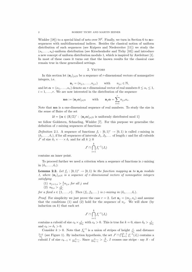
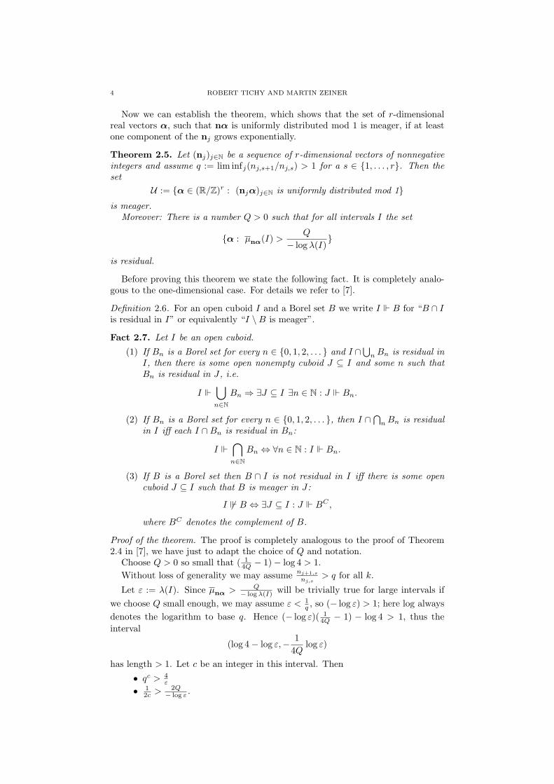
Proof. For simplicity we just prove the case r = 2. Let nj = (mj , nj) and assumethat the conditions (1) and (2) hold for the sequence of nj . We will show (byinduction on k) that each set

J ′ ∩k⋂i=1

f−1i (Ji)

contains a cuboid of size ck× ε2nk

with ck > 0. This is true for k = 0, since δ2 > ε2n0

and c0 := δ1 > 0.Consider k > 0. Note that f−1

k is a union of stripes of height εnk

and distance1−εnk

(see Figure 1). By induction hypothesis, the set J ′ ∩⋂k−1i=1 f

−1i (Ji) contains a

cuboid I of size ck−1 × ε2nk−1

. Since ε2nk−1

> 2nk

, I crosses one stripe - say S - of

BAIRE RESULTS OF MULTISEQUENCES 3

k1/m k2/m k3/m

k3/n

0 1

1

k

k

1/n

2/n

{k/nε

Figure 1.

height εnk

. Thus I ∩S contains a cuboid I ′ of size ck × ε2nk

for some ck ≤ ck−1 (seeFigure 2). �

k1/m k2/m k3/m

k/nε {

0 1

1

k

k

k

1/n

2/n

3/n

I

SI’

Figure 2.

To be able to state the theorem, we need the following definitions.

Definition 2.3. For a sequence x = (xn)n∈N of real numbers we define the measuresµx,n by

µx,n =1n

n∑i=1

δxi,

where δx denotes the point measure in x. The set of accumulation points of thesequence (µx,n)n∈N is denoted by M(x) and is called the set of limit measures ofthe sequence x.

Definition 2.4. For any sequence x = (xn)n∈N and any interval I we define µx(I)by

µx(I) := sup{µ(I) : µ ∈M(x)}.


Now we can establish the theorem, which shows that the set of r-dimensionalreal vectors α, such that nα is uniformly distributed mod 1 is meager, if at leastone component of the nj grows exponentially.

Theorem 2.5. Let (nj)j∈N be a sequence of r-dimensional vectors of nonnegativeintegers and assume q := lim infj(nj,s+1/nj,s) > 1 for a s ∈ {1, . . . , r}. Then theset

U := {α ∈ (R/Z)r : (njα)j∈N is uniformly distributed mod 1}is meager.

Moreover: There is a number Q > 0 such that for all intervals I the set

{α : µnα(I) >Q

− log λ(I)}

is residual.

Before proving this theorem we state the following fact. It is completely analo-gous to the one-dimensional case. For details we refer to [7].

Definition 2.6. For an open cuboid I and a Borel set B we write I B for “B ∩ Iis residual in I” or equivalently “I \B is meager”.

Fact 2.7. Let I be an open cuboid.

(1) If Bn is a Borel set for every n ∈ {0, 1, 2, . . . } and I ∩⋃nBn is residual in

I, then there is some open nonempty cuboid J ⊆ I and some n such thatBn is residual in J , i.e.

I ⋃n∈N

Bn ⇒ ∃J ⊆ I ∃n ∈ N : J Bn.

(2) If Bn is a Borel set for every n ∈ {0, 1, 2, . . . }, then I ∩⋂nBn is residual

in I iff each I ∩Bn is residual in Bn:

I ⋂n∈N

Bn ⇔ ∀n ∈ N : I Bn.

(3) If B is a Borel set then B ∩ I is not residual in I iff there is some opencuboid J ⊆ I such that B is meager in J :

I 6 B ⇔ ∃J ⊆ I : J BC ,

where BC denotes the complement of B.

Proof of the theorem. The proof is completely analogous to the proof of Theorem2.4 in [7], we have just to adapt the choice of Q and notation.

Choose Q > 0 so small that ( 14Q − 1)− log 4 > 1.

Without loss of generality we may assume nj+1,s

nj,s> q for all k.

Let ε := λ(I). Since µnα > Q− log λ(I) will be trivially true for large intervals if

we choose Q small enough, we may assume ε < 1q , so (− log ε) > 1; here log always

denotes the logarithm to base q. Hence (− log ε)( 14Q − 1) − log 4 > 1, thus the

interval

(log 4− log ε,− 14Q

log ε)

has length > 1. Let c be an integer in this interval. Then

• qc > 4ε

• 12c >

2Q− log ε .


Now suppose that the theorem ist false. Since the set {α : µnα(I) > Q− log ε} is a

Borel set and not residual, its complement is residual in I ′, for some open cuboidI ′:

I ′

{α : µnα(I) ≤ Q

− log ε

}.

Since µnα(I) ≥ lim supn→∞ µnα,n the set {α : µnα(I) ≤ Q− log ε} is contained in

the set {α : ∃m ∀N ≥ m : µnα,N (I) ≤ 2Q

− log ε

}.

Denote the set {j < N : njα ∈ I} by ZN (α). So µnα,N (I) = #ZN (α)N . Therefore

I ′ ⋃m

⋂N≥m

{α :

#ZN (α)N

≤ 2Q− log ε

}.

So, by Fact 2.7, we can find an open cuboid J ⊆ I ′ and a k∗ such that

J ⋂

N≥k∗

{α :

#ZN (α)N

≤ 2Q− log ε

},

or equivalently, for all N ≥ k∗:

J

{α :

#ZN (α)N

≤ 2Q− log ε

},(1)

Let δi := λi(J), where λi(J) is the length of the egde in the i-th dimension. Withoutloss of generality we assume nk∗c,s >

ε2δs

(otherwise we just increase k∗). Nowconsider the functions fk∗c, f(k∗+1)c, . . . , f(2k∗−1)c, defined as in Lemma 2.2. Since

n(k∗+i+1)c,s

n(k∗+i)c,s≥ qc > 4

ε

and nk∗c,s >εδs

, these functions are ε-mixing in (δ1, . . . , δr) by Lemma 2.2. Sothere is an open cuboid K ⊆ J such that for all α ∈ K and all i ∈ {0, . . . , k∗}:

α ∈ f−1(k∗+i)c(I) i.e. n(k∗+i)cα ∈ I.

Hence for all α ∈ K#Z2k∗c(α) = #{i < 2k∗c : niα ∈ I} ≥ #{k∗c, (k∗ + 1)c, . . . , (2k∗ − 1)c} = k∗.

So for all α ∈ K#Z2k∗c(α)

2k∗c≥ 1

2c.(2)

Since 12c >

2Q− log ε and K ⊆ J , (1) with N := 2k∗c implies

K

{α :

#Z2k∗c(α)2k∗c

≤ 12c

}.(3)

Now consider the set {α : #Z2k∗c(α)2k∗c < 1

2c} ∩ K. By (2), this set is empty, butby (3) it is residual in K, which is a contradiction. �

Note that the above theorem still remains true, if we require instead of q :=lim infj(nj,s+1/nj,s) > 1 for a s ∈ {1, . . . , r} only that there exists s ∈ {1, . . . , r}and a constant C with ∣∣{j : 2r ≤ nj,s < 2r+1

}∣∣ ≤ C ∀r.Then you can choose each c := 2Cd2− log2 εe-th term to obtain a growth of factor4/ε, and Q has to be chosen so small, that 1

2c >2Q− log ε . Indeed, one can use instead

of the base 2 in the above condition any number K > 1, but we will state alltheorems in terms of the base 2 throughout this paper.


Remark 2.8. With the same argument as above, Theorem 2.4 in [7] holds also forsequences (nj)j∈N with ∣∣{j : 2r ≤ nj < 2r+1

}∣∣ ≤ C ∀r.

So far we gave sufficient conditions that nα is u.d. mod 1 only for α in a set offirst category. If we weaken the growth condition in the following way, there will besequences n, such that nα is u.d. mod 1 for α in a set of second category. Thereforwe start with an extension of a result due to Ajtai, Havas, Komlos [2].

Lemma 2.9. Given any r sequences (εj,k)j∈N, 1 ≤ k ≤ r, εj,k ≥ 0, limj→∞ εj,k =0 for all k, there is a sequence of r-dimensional vectors of nonnegative integers(nj)j∈N with

nj+1,k

nj,k> 1 + εj,k 1 ≤ k ≤ r

such that for all α with∑ri=1 αi 6∈ Q the sequence nα is u.d. mod 1.

Proof. Set εj := max{εj,k : 1 ≤ k ≤ r}. Then, by [2, Lemma 1], there existsa sequence (nj)j∈N with nj+1/nj > 1 + εj such that njα is u.d. mod 1 for allirrational α. Define nj := (nj , . . . , nj). Then

njα =r∑i=1

njαi = nj

r∑i=1

αi = njα′

with irrational α′. �

To get a statement in Baire’s categories, we need a lemma which tells us thatthe set of d-dimensional real vectors, which entries are linearly independet over Q,is residual in Rd.

Lemma 2.10. The set

I := {α : 1, α1, . . . , αd are linearly independent over Q}is residual, and hence of second category, in Rd.

Proof. Note thatI = Rd \

⋃a0,...,ad∈Q

(a0,...,ad)6=(0,...,0)

S(a1, . . . ad)

whereS(a1, . . . ad) = {α : a0 + a1α1 + · · ·+ adαd = 0} .

Since S(a1, . . . ad) is a subspace of dimension smaller than d, all these sets S(a1, . . . ad)are nowhere dense. Therefore ⋃

a0,...,ad∈Q(a0,...,ad)6=(0,...,0)

S(a1, . . . ad)

is of first category. �

Consequently we have

Theorem 2.11. Given any r sequences (εj,k)j∈N, 1 ≤ k ≤ r, εj,k ≥ 0, limj→∞ εj,k =0 for all k, there is a sequence of r-dimensional vectors of nonnegative integers(nj)j∈N with

nj+1,k

nj,k> 1 + εj,k 1 ≤ k ≤ r

such that the set{α : nα is u.d. mod 1}

is residual.


In [7] Goldstern, Schmeling and Winkler also proved, that if the sequence (nj)j∈Ngrows very fast (i.e. if limj→∞ nj+1/nj = ∞), then the set of α, for which nα ismaldistributed, is residual. A sequence x = (xn)n∈N is called maldistributed, iffthe set M(x) is the whole set of Borel probability measures on [0, 1]. It is as easyas the modification of the proof of [7, Theorem 2.4] to the proof of Theorem 2.5 toobtain a generalisation of [7, Theorem 2.6]:

Theorem 2.12. Let (nj)j∈N be a sequence of r-dimensional vectors of nonnegativeintegers and assume that there is a s ∈ {1, . . . , r} such that limk→∞ ns,k+1/ns,k =∞. Then the set

{α ∈ (R/Z)r : nα is maldistributed}is residual.

3. nα-sequences in Rd

In this section we investigate in uniform distribution in Rd. For a sequence(nj)j∈N of d-dimensional vectors of nonnegative integers and a d-dimensional vectorα = (α1, . . . , αd) of real numbers we are interested in the sequence

nα := (nj,1α1, . . . , nj,dαd)j∈N.

To obtain results for such sequences we use the connection between uniform dis-tribution modulo 1 in [0, 1]d and uniform distribuion in [0, 1]. As in the previoussection our first theorem shows that the set of α such that nα is u.d. is meager ifat least one component of the nj grows exponentially.

Theorem 3.1. Let (nj)j∈N be a sequence of d-dimensional vectors of nonnegativeintegers and assume that there exists s ∈ {1, . . . , d} and a constant C with∣∣{j : 2r ≤ nj,s < 2r+1

}∣∣ ≤ C ∀r.

ThenA :=

{α ∈ (R/Z)d : nα is u.d. mod 1 in Rd

}is meager.

Proof. By [11, Theorem 6.3], uniform distribution of nθ implies that each compo-nent niθi := (nj,iθi)j∈N, 1 ≤ i ≤ d is u.d. mod 1, especially nsθs is u.d. mod 1.Therefore

A ⊆ R× · · · × R×As × R× · · · × R,where

As := {θ : nsθ u.d. mod 1} .By Remark 2.8, the set As is meager. Hence, by [15, Th. 15.3.], A is meager. �

As before the grows condition in the theorem above cannot be weakened:

Lemma 3.2. Given any d sequences (εj,k)j∈N, 1 ≤ k ≤ d, εj,k ≥ 0, limj→∞ εj,k =0 for all k, there is a sequence of d-dimensional vectors of nonnegative integers(nj)j∈N with

nj+1,k

nj,k> 1 + εj,k 1 ≤ k ≤ d

such that for all α with 1, α1, . . . , αd linearly independent over Q the sequence(nj,1α1, . . . , nj,dαd)j∈N is u.d. mod 1 in Rd.

Proof. Set εj := max{εj,k : 1 ≤ k ≤ d}. Then, by [2, Lemma 1], there existsa sequence (nj)j∈N with nj+1/nj > 1 + εj such that njα is u.d. mod 1 for allirrational α. Define nj := (nj , . . . , nj). By [11, Theorem 6.3] we have to show that


for all h ∈ Zd, h 6= 0 the sequence 〈h, njα〉 is u.d. mod 1 for all α with 1, α1, . . . , αdlinearly independent over Q. This is true since

〈h, njα〉 =d∑i=1

hinjαi = nj

d∑i=1

hiαi = njα′

with α′ ∈ R \Q. �

Using Lemma 2.10 we get as an immediate consequence

Theorem 3.3. Given any d sequences (εj,k)j∈N, 1 ≤ k ≤ d, εj,k ≥ 0, limj→∞ εj,k =0 for all k, there is a sequence of d-dimensional vectors of nonnegative integers(nj)j∈N with

nj+1,k

nj,k> 1 + εj,k 1 ≤ k ≤ d

such that the set{α : (nj,1α1, . . . , nj,dαd)j∈N is u.d. mod 1 in Rd

}is residual.

Again using [15, Th. 15.3.] we obtain for fast growing sequences (nj):

Theorem 3.4. Let (nj)j∈N be a sequence of d-dimensional vectors of nonnegativeintegers and assume limk→∞ nt,k+1/nt,k =∞ for all t ∈ {1, . . . , d}, then the set

{α ∈ (R/Z)d : nα is maldistributed}is residual.

We can combine the ideas of this and the previous section: Consider a sequenceof d× r-matrices of nonnegative integers

(Nj)j∈N with Nj = (njik), i = 1, . . . , d, k = 1, . . . , r.

We are now interested in the distribution of the sequence Nα := (Njα)j∈N, whereNjα means the classical matrix-vector-product. Same argumentation as in theproof of Theorem 3.1 yields

Theorem 3.5. Let (Nj)j∈N be a sequence of d×r-matrices of nonnegative integersand assume that there exist s ∈ {1, . . . , d}, t ∈ {1, . . . , r} and a constant C with∣∣∣{j : 2r ≤ njst < 2r+1

}∣∣∣ ≤ C ∀r.

Then the set

A :={α = (α1, . . . , αr) : Nα is u.d. mod 1 in Rd

}is meager.

4. Uniform distribution of nets

In this section we define uniform distribution of nets of elements of a locallycompact Hausdorff space and give a list of some elementary properties which gen-eralise the results for classical sequences given in Bauer [3], Helmberg [8], Kuipersand Niederreiter [11] and Winkler [18]. The proofs are analogous to the ones of thecase of one-dimensional sequences, so we omit them and just state the theorems. Asexplained in the following such nets induce nets of certain discrete probability mea-sures. Uniform distribution properties of nets of general probability measures onlocally compact groups were studied in Gerl [5] and Maxones and Rindler [13, 14].A special kind of nets are sequences indexed by d-dimensional vectors in Nd. Suchsequences of random variables also appear in probability theory, see eg. Jacod andShiryaev [9]. For an introduction to nets we refer to Willard [17].


Throughout this and the following section let X 6= ∅ be a locally compact Haus-dorff space with countable topology base. Moreover, letM(X) be the compact setsof nonnegative finite Borel measures with µ(X) = 1 if X is compact and µ(X) ≤ 1if X is not compact, equipped with the topology of weak convergence. On M(X)we use the metric given in [18]. Furthermore let Λ (equipped with a relation ≤)be a countable directed set with the additional property that for all λ ∈ Λ the setV(λ) := {ν : ν ≤ λ} is finite.

For net x = (xλ)λ∈Λ of elements in X and a function f ∈ K(X), the space ofall continuous real-valued functions on X whose support is compact, we define thenet µf = (µλ,f )λ∈Λ by

(4) µλ,f =1

|V(λ)|∑`≤λ

f(x`).

If the nets µf converges to the integral∫X

fdµ

for all f ∈ K(X) then we say x is µ-uniformly distributed (µ-u.d.) in X.Now we give some basic properties:

(i) If V is a class of functions from K(X) such that sp(V ) is dense in K(X),then V is convergence-determining with respect to any µ in X.

(ii) If sp(V ) is a subalgebra ofK(X) that seperates points and vanishes nowhere,then V is a convergence-determining class with respect to any µ in X.

(iii) The net x = (xλ)λ∈Λ is µ-u.d. in X iff the nets yM = (yMλ )λ∈Λ defined by

yMλ =A(M ;λ)|V(λ)|

converge to µ(M) for all compact µ-continuity setsM ⊆ X. HereA(M ;λ) =∑`≤λ 1M (x`).

(iv) In a locally compact Hausdorff space X with countable space, there exists acountable convergence-determining class of real-valued continuous functionswith compact support with respect to any µ ∈M(X).

(v) Let S be the set of all µ-u.d. sequences in X, viewed as a subset of XΛ :=∏λ∈Λ. Then µ∞(S) = 1.

(vi) If X contains more than one element, then the set S from the above theoremis a set of first category in XΛ.

(vii) The set S is everywhere dense in XΛ.Generalising the concept of uniform distribution we introduce the set M(x), the

set of limit measures of the net x, as the set of cluster points of the net µ = (µλ)λ∈Λ

of induced measures defined by

(5) µλ =1

|V(λ)|∑`≤λ

δx`.

If M(x) = {µ} (µ ∈ M(X)), then this net is µ-u.d. in X. If M(x) = M(X) wesay x is maldistributed in X.

As in the classical case (see [18]) only very few (in a topological sense) nets areµ-u.d. Moreover, almost all nets are maldistributed. We have:The typical situation in the sense of Baire is M(x) =M(X), i.e. the set

Y = {x ∈ XΛ| M(x) =M(X)} ⊆ XΛ

is residual.


At the end of this section we define two notions of uniform distribution onΛ = Nd, which we will use in the following. First let Nd be equipped with therelation ≤ defined by x ≤ y iff xi ≤ yi (1 ≤ i ≤ d). The second concept is tointroduce the relation ≤s defined by x ≤s y iff |x| ≤ |y|, where |x| :=

∏di=1 xi. A

µ-u.d. net w.r.t. to this relation on Nd we will call strongly uniformly distributed(s.u.d.). The set of limit measure we denote by Ms(x). The first concept is inaccord with Kuipers and Niederreiter [11], the second concept is motivated byAistleitner [1], who studied the discrepancy of sequences with multidimensionalindices.

5. Characterisation of M(x) and distribution of subnets for aspecial kind of nets on Nd

This section is devoted to the generalisation of the characterisation of the sets oflimit measures given in Winkler [18, Theorem 3.1] to nets defined on Λ = (Nd,≤)(see Section 4).

To simplify notation we introduce some operations on multidimensional indices.For an index i = (i1, . . . , id) we define

i + c = (i1 + c, . . . , id + c)

i mod c = (i1 mod c, . . . , id mod c).

Furthermore, we define the index-sets

I[i, j] := {k : k ≥ i and ∃` : k` ≤ j`}I[i, j) := {k : k ≥ i and ∃` : k` < j`} = I[i, j− 1]

I(i, j] := {k : k > i and ∃` : k` ≤ j`} = I[i + 1, j].

A sequence of the form x = (xi)i∈I[1,N] we call an angle-sequence, and by theperiodic continuation of an angle-sequence by a finite sequence y = (yi)1≤i≤N1 wemean the sequence x′ = (x′i)i∈Nd defined by

x′i ={xi if i ∈ I[1,N]yki−N mod N1

if i > N .

Here we assume N = (N, . . . , N) and N1 = (N1, . . . , N1). In fact, we could definethe above construction for arbitrary indices N and N1, but in the following we willjust need this definition.

Example 5.1. In two dimensions the periodic continuation of x with period y lookslike the following:

......

...... . .

.

... y y y · · ·

... y y y · · ·

... y y y · · ·x · · · · · · · · · · · ·

The following lemma generalises [18, Section 2] and gives some properties of theset M(x).

Lemma 5.2. For all sequences x ∈ Xω×···×ω the set M(x) has the following prop-erties: M(x) is

(i) nonempty,(ii) contained in M(X),(iii) closed (hence compact),


(iv) connected.

Proof. (i): M(x) 6= ∅ since every net in a compact space has a convergent subnetand all λN ∈M(X).

(ii): The proof is completely analogous to the proof in [18], you just have to takethe multidimensional limit.

(iii): M(x) is the set of cluster points of the net y = (yN)N∈Nk , and the set ofcluster points of any net in any topological space is closed.

(iv): Assume that M = M(x) is not connected. Therefore there are nonemptydisjoint closed subsets M1, M2 ⊆M with M = M1 ∪M2. Since compact Hausdorffspaces are normal, we can find open sets Oi and Vi, i = 1, 2, in M(X) satisfying

Mi ⊆ Oi ⊆ Oi ⊆ Vi, i = 1, 2, and V1 ∩ V2 = ∅.Thus the closures of the Oi are compact and disjoint. This yields that they havepositive distance

d(O1, O2) = infµi∈Oi

d(µ1, µ2) = ε > 0.

Now consider the compact set L =M(X)\O1 \O2. Since both M1 and M2 containcluster points of Λ, the net has to be infintely many times in O1 as well as inO2 for all tails (λN)N≥n with n ∈ Nd. Observe that d(λN, λN+1) ≤ c/(N + 1),where N = (N, . . . , N). Thus the distance of subsequent members in the diagonalof Λ gets arbitrarily small, say less than ε. This means that Λ has to intersect Linfinitely many times for all tails (λN)N≥n with n ∈ Nd. Since L is compact, theremust be a cluster point of Λ in L, but we also have

L ∩M = L ∩ (M1 ∪M2) ⊆ (L ∩O1) ∪ (L ∩O2) = ∅,which is a contradiction. �

The parts (i), (ii), and (iii) of the lemma above are valid for arbitrary nets asconsidered in Section 4, whereas part (iv) fails in general. We give the followingexample: Let x = (xn,m)(n,m)∈N2 be the net defined by

x(n,m) ={

0 if m = 01 if m > 0

and consider the relation ≤s. Then the set of limit measures is the set

M(x) = {λ : λ(0) = 1n , λ(1) = 1− 1

n} ∪ {δ1}.Now we turn to the main result of this section. The proof uses two lemmas which

we will present afterwards. With the definitions given in Section 4 we have

Theorem 5.3. Let X be a locally compact Hausdorff space with countable topolog-ical base and x = (xn)n∈Nd a net. Then:

(1) Every M(x) is a nonempty, closed (hence compact) and connected subsetof M(X).

(2) Let M ⊆M(X) be nonempty, compact and connected. Then there is a netx ∈ Xω×···×ω with M(x) = M .

Proof. (1) see Lemma 5.2(2) By Lemma 5.4 there exists a net (µk)k∈Nd in M whose set of cluster points

equals M and with the additional property that limk→∞ εk = 0 with a monotoni-cally nonincreasing sequence of εk > dk where dk is the maximum of the distances ofµk to its successors (see Lemma 5.4). Now we construct a sequence x = (xn)n∈Nd

such that the induced sequence of the λN approximates the µk in the followingsense: There are indices N1 < N2 < · · · such that d(µ, λN(x)) < 2εk for allN ∈ I[Nk,Nk+1) where Nj = (Nj , . . . , Nj). Then the relation M = M(x) is animmediate consequence.


To construct such a sequence we take a finite sequence x0 = (x0i )1≤i≤N0 such

that d(λN0(x0), µ1) < ε1 (the existence of x0 is guaranteed by Section 4). Considerthe sequence x1 = (x1

i )i∈Nd with x1i = xi mod N0 such that there is a number N1

with d(λN(x1), µ1) < ε1 for all N ≥ N1. Now we proceed by induction:For arbitrary k ≥ 1 assume that there is an angle-sequence xk = (xki )i∈I[1,Nk]

with the following properties:

(1) d(λNk(xk), µk) < εk.

(2) There is a finite sequence yk = (yki )1≤i≤(K,...,K) such that for the periodiccontinuation xck of xk with period yk we have d(λN(xck), µk) < εk for allN ≥ Nk.

By Lemma 5.6 there is an angle-sequence x′ = (x′i)i∈I(Nk,Nk+1] such that for theangle-sequence xk+1 = (xk+1

i )i∈I[1,Nk+1] defined by

xk+1i =

{xki if i ∈ I[1,Nk]x′i if i ∈ I(Nk,Nk+1]

the following conditions hold:

(i) If N ∈ I[Nk,Nk+1), then there is a point µ on the linear connection betweenµk and µk+1 with d(λN(xk+1), µ) < Cεk, where C is a constant dependingonly on the dimension d.

(ii) There is a finite sequence yk+1 = (yk+1i )1≤i≤(K′,...,K′) such that for the

periodic continuation of xk+1 with yk+1, which we denote by x, we haved(λN(x), µk+1) < εk+1 for all N ≥ Nk+1.

Then the limit sequence limk→∞ xk+1, generated by the above induction, has thedesired properties. �

Lemma 5.4. Let M be a nonempty closed and connected subset of M(X). Thenthere is a net (µk)k∈Nd in M , whose set of cluster points equals M and with theadditional properties limk→∞ dk = 0, where dk is the maximum of the distancesof µk to its successors, i.e. dk = maxk′∈Ik d(µk, µk′), where Ik = {(K1, . . . ,Kd) :Ki ∈ {ki, ki + 1}, i = 1, . . . , d} if k = (k1, . . . kd), and µk′ = µ(k,k,...,k), where k′

runs over all indices which coincide with (k, . . . , k) in at least one coordinate.

Example 5.5. In two dimensions such a net has the following form:...

......

...... . .

.

µ1 µ2 µ3 µ4 µ5 · · ·µ1 µ2 µ3 µ4 µ4 · · ·µ1 µ2 µ3 µ3 µ3 · · ·µ1 µ2 µ2 µ2 µ2 · · ·µ1 µ1 µ1 µ1 µ1 · · ·

Proof. By [18, Lemma 3.3], there exists a sequence (µk)k∈N in M whose set of accu-mulation points equals M and with limk→∞ d(µk, µk+1) = 0. The net determinedby µ(k,...,k) = µk has the desired properties. �

Lemma 5.6. Let µk, µk+1 ∈ M(X) and εk > εk+1 > 0 be given. Assume thatxk = (xki )i∈I[1,Nk] with Nk = (Nk, . . . , Nk) is an angle-sequence with the followingproperties:

(1) d(λNk(xk), µk) < εk

(2) There exists a finite sequence yk = (yki )1≤i≤(K,...,K) such that for the pe-riodic continuation xck of xk with period yk the following property holds:d(λn(xck), µk) < εk for all n ≥ Nk.


Then there is an angle-sequence x′ = (x′i)i∈I(Nk,Nk+1] such that for the angle-sequence xk+1 = (xk+1

i )i∈I[1,Nk+1] defined by

xk+1i =

{xki if i ∈ I[1,Nk]x′i if i ∈ I(Nk,Nk+1]

the following conditions hold:(i) If n ∈ I[Nk,Nk+1) then there is a point µ on the linear connection between

µk and µk+1 with d(λn(xk+1), µ) < Cεk, where the constant C dependsonly on the dimension d.

(ii) There is a finite sequence yk+1 = (yk+1i )1≤i≤(K′,...,K′) such that for the

sequence x, which denotes the periodic continuation of xk+1 with periodyk+1, we have d(λn(x), µk+1) < εk+1 for all n ≥ Nk+1.

Proof. By Section 4 there is a sequence y with limit distribution µk+1. Take theinitial part yk+1 = (yk+1

i )1≤i≤(K′,...,K′) in such a way that the induced measureλ = λ(K′,...,K′)(yk+1) satisfies

d(λ, µk+1) < εk+1 < εk

and K|K ′. Consider the angle-sequence xk+1 = (xk+1i )i∈I[1,Nk+1] constructed in

the following way:

xk+1i =

xki if i ∈ I[1,Nk]yki−Nk mod K if i ∈ I(Nk,Nk +mkK]yi−(Nk+mkK) mod K′ if i ∈ I(Nk +mkK,Nk+1]

,

where Nk+1 = (Nk+1, . . . , Nk+1) and Nk+1 = Nk + mkK + mk+1K′ with suit-

able chosen mk and mk+1; this is done below. Let x denote the sequence ob-tained from xk+1 by periodic continuation with period yk+1. We first prove thesecond statement of the lemma. Given mk, we can choose mk+1 large enoughthat d(λn(x), µk+1) < εk+1 for all n ≥ Nk+1 since for n = (n1, . . . , nd) withni = Nk +mkK +mk+1K

′ + siK′ + ci with 0 ≤ ci < K ′ and si ≥ 0 we have

d(λN(x), µk+1) = d

(1|n|

(K ′d

d∏i=1

(mk+1 + si)λ+∑)

, µk+1

)

≤ 1|n|

K ′dd∏i=1

(mk+1 + si)d(λ, µk+1)

+|n| −K ′d

∏di=1(mk+1 + si)|n|

= 1− (1− d(λ, µk+1))1|n|

K ′dd∏i=1

(mk+1 + si),

where∑

is a sum over |n| −K ′d∏di=1(mk+1 + si) indicator functions. For mk+1

so large that1|n|

K ′dd∏i=1

(mk+1 + si) >1− εk+1

1− d(λ, µk+1),

the statemant is true.Now we turn to the first assertion. Firstly we give a detailed proof of the two-

dimensional case, afterwards we prove the general case. Indeed, the general caseuses the same idea as the two-dimensional case, but it is not necessary (and inhigher dimension also very awful to write things down) to be so accurate as we arein the two-dimensional case, but this accuracy will be very helpful to understandwhat’s going on.


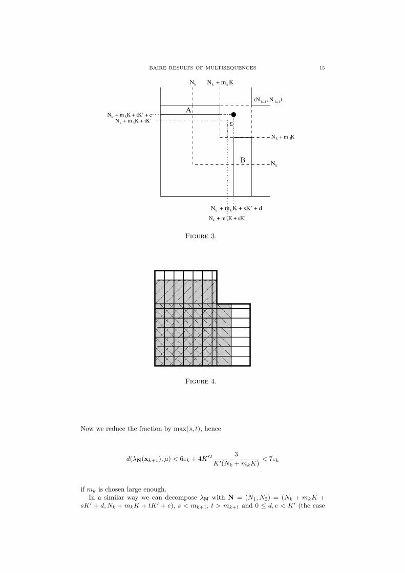
So we have to show that for all n ∈ I[Nk,Nk+1) we have d(λn(xk+1), µ) < Cεkfor some µ on the linear connection between µk and µk+1. For n ∈ I[N,Nk+mkK]this is true by assumption. Now consider a point N = (N1, N2) = (Nk + mkK +sK ′ + d,Nk + mkK + tK ′ + e) with 0 ≤ s, t ≤ mk+1 and 0 ≤ d, e < K ′. We canwrite λN as

NλN = N2k+1

st

m2k+1

λNk+1

− (Nk +mkK)(Nk +mkK +mk+1K′)

st

m2k+1

λ(Nk+mkK,Nk+1)

− (Nk +mkK)(Nk +mkK +mk+1K′)

st

m2k+1

λ(Nk+1,Nk+mkK)

+ (Nk +mkK)(Nk +mkK + tK ′ + e)λ(Nk+mkK,N2)

+ (Nk +mkK)(Nk +mkK + sK ′ + d)λ(N1,Nk+mkK)

+(

st

m2k+1

− 1)

(Nk +mkK)2λ(Nk+mkK,Nk+mkK)

+∑

=: a1λ1 +6∑i=2

aiλi +∑

,

where∑

is a sum over de+esK ′+dtK ′ indicator functions. The first term is neededto count the indicator functions induced by the complete yk+1-blocks. In λNk+1 wehave m2

k+1 such blocks and we need st blocks, so we multiply with stm2

k+1. But with

this measure we count too many indicator functions, namely those in the areas A =I((1, N2), (Nk+mkK,Nk+1)] and B = I((N1, 1), (Nk+1, Nk+mkK)] (see Figure 3).This error is corrected by subtracting the terms with the measures λ(Nk+mkK,Nk+1)

and λ(Nk+1,Nk+mkK). But now we have eliminated all contributions from the areasI((1, Nk + mkK), (Nk + mkK,N2)] and I((Nk + mkK, 1), (N1, Nk + mkK)] too,so we add the terms with λ(Nk+mkK,N2) and λ(N1,Nk+mkK). Last we correct thecontribution of I[1, (Nk + mkK,Nk + mkK)]. The measure

∑contains all the

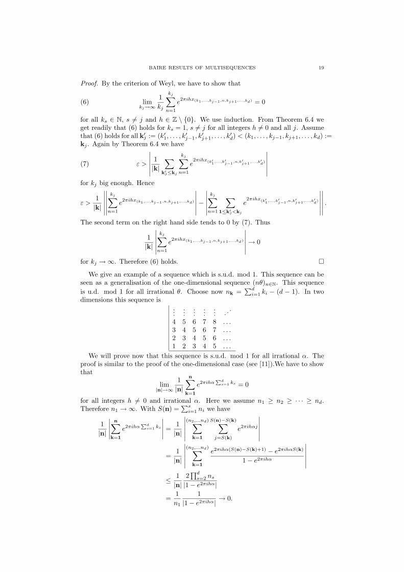
indicator functions from the incomplete yk+1-blocks.Figure 4 illustrates this procedure (except the error

∑): We have the thick-

border area and want to construct the grey area, using only rectangles startingin the origin. So we substract the vertical and horizontal dotted areas first, thenwe have to add their intersection, the thick-borderd square again. Afterwards weadd the diagonally lined areas and correct the error we made by substracting theirintersections, again thick-borderd square.

Now define µ := 1|N|

(a1µk+1 + µk

(∑6i=2 ai + de+ dtK ′ + esK ′

)). Then µ is

on linear connection between µk and µk+1 and we have

d(λN(xk+1), µ) ≤ a1d

N1N2(λ1(xk+1), µk+1) +

1N1N2

6∑i=2

|ai|d(λi(xk+1), µk)

+ 2de+ dtK ′ + esK ′

N1N2

< 6εk + 22K ′2(s+ t+ 1)

N1N2


N + m K + sK’ + dk k

k+1(N , N )

k+1

N + m Kk k

Nk

N + m Kk kNk

N + m K + sK’k k

N + m K + tK’ + ek k

N + m K + tK’k k

A

B

Σ

Figure 3.

Figure 4.

Now we reduce the fraction by max(s, t), hence

d(λN(xk+1), µ) < 6εk + 4K ′23

K ′(Nk +mkK)< 7εk

if mk is chosen large enough.In a similar way we can decompose λN with N = (N1, N2) = (Nk + mkK +

sK ′ + d,Nk + mkK + tK ′ + e), s < mk+1, t > mk+1 and 0 ≤ d, e < K ′ (the case


t < mk+1, s > mk+1 is symmetric) into

N1N2λN = Nk+1(Nk +mkK + (t+ 1)K ′)st

mk+1(t+ 1)λ(Nk+1,Nk+mkK+(t+1)K′)

− st

mk+1(t+ 1)(Nk +mkK)(Nk +mkK + (t+ 1)K ′)λ(Nk+mkK,Nk+mkK+(t+1)K′)

− st

mk+1(t+ 1)Nk+1(Nk +mkK)λ(Nk+1,Nk+mkK)

+ (Nk +mkK)N2λ(Nk+mkK,N2)

+N1(Nk +mkK)λ(N1,Nk+mkK)

+(

st

mk+1(t+ 1)− 1)

(Nk +mkK)2λ(Nk+mkK,Nk+mkK)

+∑

,

where∑

is a sum over de + esK ′ + dtK ′ indicator functions and obtain that forsuitable chosen µ on the linear connection between µk and µk+1

d(λN(xk+1), µ) < 7εk.

Now we turn to the general case. Therefor consider a point N = (N1, . . . , Nd)with Ni = Nk +mkK + siK

′ + di and si < mk+1 and 0 ≤ di < K ′ first. Then wecan write

|N|λN = |Nk+1|∏di=1 si

mdk+1

λNk+1 +T∑i=1

aiλni +∑

,

where ni is of the form ni = (n1, . . . nd) with all ni ∈ {Nk+1, Nk + mkK} or allni ∈ {Ni, Nk + mkK} but not all ni = Ni. The coefficients ai = vi|ni|ci with

vi ∈ {1,−1} and ci ∈ {1,Qd

i=1 si

mdk+1}. The above formula is true, since after taking

λNk+1 , we have to substract the error we made. Therefore we substract the λni

with exactly one ni = Nk + mkK and for all the other j 6= i with nj = Nk+1;there are p1 = d such measures. Each two of them have an intersection, so we havethe correct this, which leads to p2 =

(d2

)summands (each such index has exactly

two entries Nk + mkK). Each of them have again an intersection (now there arep3 =

(p22

)of them) and so on (pi+1 =

(pi

2

)). After d steps this procedure must end.

Afterwards we start adding the terms with those ni with exactly one entry equalsNk +mkK and the other entries equal Ni. There are p1 of them. Then we correctthe intersections again and so on. Last we add the term due to the non-completeyk blocks, this is denoted by

∑and is a sum over

S := 1 +d∑j=1

∑A⊆{1,...,d}|A|=j

K ′d−j∏p∈A

dp∏

q∈{1,...,d}\A

sq

indicator functions.Hence T ≤ 2

∑di=1 pi < F (d), where F (d) is a constant only depending on the

dimension d. Taking

µ =1N|Nk+1|

∏di=1 si

mdk+1

µk+1 +1N

(T∑i=1

ai + S

)µk

we find that

d(λN(xk+1), µ) ≤ F (d)εk +2S|N|

.


By reducing the fraction on the right-hand side by the product of the (d−1) greatestsi and estimating di ≤ K ′ we see

d(λN(xk+1), µ) ≤ F (d)εk + 22dK ′d

K ′d−1(Nk +mkK).

So we have to choose mk in such a way that the fraction becomes small. A similarconstruction holds for the other points N ∈ I[Nk +mkK,Nk+1) . �

After this characterisation of M(x) we will study the distribution of certain sub-nets of a given net and generalise results due to Goldstern, Winkler and Schmel-ing [6]. We study subnets as studied in Losert and Tichy [12]: Choose d sequencesa1, . . . ,ad ∈ {0, 1}N and define a = (an)n∈Nd by

a(n1,...,nd) =d∏i=1

ai,ni.

Then the subnet ax of x is the net obtained by taking those elements xn for whichan = 1 and using the given relation ≤.

The next theorem is a consequence of Theorem 5.3 and generalises [6, Theorem1.2]:

Theorem 5.7. Let x ∈ XNd

and M ⊆M(X). Then there exists a subsequence axwith M(ax) = M iff M is closed and connected with ∅ 6= M ⊆ M(A(x)), whereA(x) is the set of cluster points of the net x.

Proof. This proof runs along the same lines as the one in [6]: First assume M =M(ax). Using Lemma 5.2 we get that M is nonempty, closed and connected. Itremains to show that M ⊆ M(A(x)). For this purpose it suffices to show thatevery x ∈ X \ A(x) has a neighbourhood U with limN→∞ µN,ax(U) = 0. Therefortake a neighbourhood U with compact closure U and with U ∩A(x) = ∅. If xn ∈ Ufor an infinite increasing sequence of indices n1 < n2 < · · · , U would contain acluster point of x, which is a contradiction. Hence xn 6∈ U for all n ≥ N0. Thus

limN→∞

µN,ax(U) ≤ limN→∞

|N0||N|

= 0.

The other direction is completely analogous to [6]. �

Similarly to [6, Theorem 1.3] we get that a typical subsequence of a given se-quence is maldistributed in A(x):

Theorem 5.8. M(ax) = M(A(x)) holds for all a ∈ R from a residual set R ⊆[0, 1)d.

6. nα-nets over Nd

In this section we specalise on nα-nets over Nd, i.e. we consider X = [0, 1)and µ the Lebesgue-measure. Besides the two notions of uniform distribution mod1 according to Section 4 we consider the (s1, . . . , sd)-u.d. (see Kirschenhofer andTichy [10]). After some elementary properties and examples of these three con-cepts we turn to the generalisation of results given in Goldstern, Schmeling andWinkler [7] and Ajtai, Havas and Komlos [2].

In Section 4 we introduced two special notions of uniform distribution. In thecontext of this section we call a net x uniformly distributed mod 1 iff for any a andb with 0 ≤ a < b ≤ 1,

limN1,...,Nd→∞

A([a, b); N)|N|

= b− a,


where A([a, b); N) is the number of xk, 1 ≤ k ≤ N with a ≤ {xk} < b.This definition is a direct extension of uniform distribution in the case d = 2

given by Kuipers and Niederreiter [11] and a special case of the concept studiedin Losert and Tichy [12]. Following [11] one gets immediately the theorems givenbelow.

Theorem 6.1. The sequence (xk)k∈Nd is u.d. mod 1 iff for every Riemann-integrable function f on [0, 1]

limN1,...,Nd→∞

1|N|

N∑k=1

f ({xk}) =

1∫0

f(x)dx,

where∑N

k=1 =∑

k:1≤k≤N.

Theorem 6.2. The sequence (xk)k∈Nd is u.d. mod 1 iff

limN1,...,Nd→∞

1|N|

N∑k=1

e2πihxk = 0

for all integers h 6= 0.

Moreover, a net x = (xk)k∈Nd is said to be strongly uniformly distributed (s.u.d.)mod 1 iff for any a and b with 0 ≤ a < b ≤ 1,

lim|N|→∞

A([a, b); N)|N|

= b− a.

Here lim|N|→∞ f(N) = f means that ∀ε > 0 ∃N ∈ N : ∀N with |N| ≥ N :|f(N)− f | < ε.

The following theorems hold:

Theorem 6.3. The sequence (xk)k∈Nd is s.u.d. mod 1 iff for every Riemann-integrable function f on [0, 1]

lim|N|→∞

1|N|

N∑k=1

f ({xk}) =

1∫0

f(x)dx.

Theorem 6.4. The sequence (xk)k∈Nd is s.u.d. mod 1 iff

lim|N|→∞

1|N|

N∑k=1

e2πihxk = 0

for all integers h 6= 0.

As in the one-dimensional case, a sequence with multidimensional sequences isstrongly uniformly distributed modulo 1 if and only if the multidimensional dis-crepancy introduced by Aistleitner [1] tends to 0.

Clearly, strong uniform distribution implies uniform distribution. The converseis not true: Consider the double sequence x defined by xj,k = jθ with θ irrational.Then this sequence is u.d. mod 1 (this follows easily from Theorem 6.2), but nots.u.d., since this sequence is constant for fixed k. Thus x is not s.u.d. mod 1 bythe following theorem:

Theorem 6.5. Let xk be s.u.d. mod 1. Then all “one-dimensional sequences”, i.e.sequences (x(k1,...,kj ,...,kd))kj∈N with fixed ks, s 6= j, are u.d. mod 1.


Proof. By the criterion of Weyl, we have to show that

(6) limkj→∞

1kj

kj∑n=1

e2πihx(k1,...,kj−1,n,kj+1,...,kd) = 0

for all ks ∈ N, s 6= j and h ∈ Z \ {0}. We use induction. From Theorem 6.4 weget readily that (6) holds for ks = 1, s 6= j for all integers h 6= 0 and all j. Assumethat (6) holds for all k′j := (k′1, . . . , k

′j−1, k

′j+1, . . . , k

′d) < (k1, . . . , kj−1, kj+1, . . . , kd) :=

kj . Again by Theorem 6.4 we have

(7) ε >

∣∣∣∣∣∣ 1|k|

∑k′j≤kj

kj∑n=1

e2πihx(k′1,...,k′

j−1,n,k′j+1,...,k′

d)

∣∣∣∣∣∣for kj big enough. Hence

ε >1|k|

∣∣∣∣∣∣∣∣∣∣∣∣kj∑n=1

e2πihx(k1,...,kj−1,n,kj+1,...,kd)

∣∣∣∣∣∣−∣∣∣∣∣∣kj∑n=1

∑1≤k′j<kj

e2πihx(k′1,...,k′

j−1,n,k′j+1,...,k′

d)

∣∣∣∣∣∣∣∣∣∣∣∣ .

The second term on the right hand side tends to 0 by (7). Thus

1|k|

∣∣∣∣∣∣kj∑n=1

e2πihx(k1,...,kj−1,n,kj+1,...,kd)

∣∣∣∣∣∣→ 0

for kj →∞. Therefore (6) holds. �

We give an example of a sequence which is s.u.d. mod 1. This sequence can beseen as a generalisation of the one-dimensional sequence (nθ)n∈N. This sequenceis u.d. mod 1 for all irrational θ. Choose now nk =

∑di=1 ki − (d − 1). In two

dimensions this sequence is...

......

...... . .

.

4 5 6 7 8 . . .3 4 5 6 7 . . .2 3 4 5 6 . . .1 2 3 4 5 . . .

We will prove now that this sequence is s.u.d. mod 1 for all irrational α. Theproof is similar to the proof of the one-dimensional case (see [11]).We have to showthat

lim|n|→∞

1|n|

n∑k=1

e2πihαPd

s=1 ks = 0

for all integers h 6= 0 and irrational α. Here we assume n1 ≥ n2 ≥ · · · ≥ nd.Therefore n1 →∞. With S(n) =

∑si=1 ni we have

1|n|

∣∣∣∣∣n∑

k=1

e2πihαPd

s=1 ks

∣∣∣∣∣ =1|n|

∣∣∣∣∣∣(n2,...nd)∑

k=1

S(n)−S(k)∑j=S(k)

e2πihαj

∣∣∣∣∣∣=

1|n|

∣∣∣∣∣∣(n2,...nd)∑

k=1

e2πihα(S(n)−S(k)+1) − e2πihαS(k)

1− e2πihα

∣∣∣∣∣∣≤ 1|n|

2∏ds=2 ns

|1− e2πihα|

=1n1

1|1− e2πihα|

→ 0.


We give another example: In the one-dimensional case the sequence ({k!e})k∈Nhas 0 as the only limit point (see [11]). Consider now the sequence nk = (S(k) −d+ 1)! =: k!. Then

k!e = A+eα

S(k)− d+ 1, 0 < α < 1, A ∈ N.

Thus {k!e} = eα/(S(k)−d+ 1)→ 0 in the first sense. Therefore it is not u.d. mod1 (and hence not s.u.d. mod 1).

The third concept is the (s1, . . . , sd)-uniform distribution introduced by Kirschen-hofer and Tichy [10]. According to the definitions above we gave an equivalentdefintion to that one stated in [10].

Definition 6.6. A sequence (xk)k∈Nd is (s1, . . . , sd)-u.d. iff for all ai1...id and bi1...idwith 0 ≤ ai1...id < bi1...id ≤ 1 and 1 ≤ ij ≤ sj for 1 ≤ j ≤ d

limN1,...,Nd→∞∏di=1

(Ni

si

)−1A ([a11...1, b11...1), . . . , [as1...sd

, bs1...sd);N1, . . . , Nd; s1, . . . sd)

=∏di=1

∏si

ji=1 bj1...jd − aj1...jdwhere A ([a11...1, b11...1), . . . , [as1...sd

, bs1...sd);N1, . . . , Nd; s1, . . . sd) is the number of

(s1 · · · sd)-tuples (xi11,...id1, . . . xi1s1 ,...idsd

) with 1 ≤ ij1 < · · · < ijsd≤ Nj for all

1 ≤ j ≤ d in [a11...1, b11...1)× · · · × [as1...sd, bs1...sd

).

As in [11] we have that the set S of (s1, . . . , sd)-u.d. sequences is everywheredense in Xω×···×ω. By [10], (s1, . . . , sd)-uniform distribution implies uniform dis-tribution. Thus from Section 4 we conclude: If X contains more than one element,then the set S of (s1, . . . , sd)−µ-u.d. sequences is a set of first category in Xω×···×ω.

After these examples and elementary properties of uniform distribution of se-quences with multidimensional indices, we turn to the generalisation of [7, Theo-rem 2.4] for these cases. For the sake of completeness we mention that in [16] Salatproved that for a sequence (nk)k∈N with nk =

∏kj=1 qj , where (qj)j∈N is a sequence

of integers greater than 1, then the set U := {α ∈ R : (nkα) is u.d.mod 1 } ismeager. By modifying the proof slightly, we get

Theorem 6.7. Let (qk)k∈Nd be a sequence of integers greater than 1. Put

an =n∏

k=1

qk, n ∈ Nd.

Then the setU := {α ∈ R : (nkα) is u.d. mod 1}

is meager. Consequently the sets

U ′ := {α ∈ R : (nkα) is s.u.d. mod 1}

andU ′′ := {α ∈ R : (nkα) is (s1, . . . , sd)-u.d.}

are meager.

Now we turn to the stronger result. We will generalise [7, Theorem 2.4]. Forthis purpose we will follow [7] again. Recall the definitions of Section 4. Moreover,let λ denote the Lebesgue measure on R/Z.

We start with an elementary property.

Theorem 6.8. Given a sequence x = (xn)n∈Nd we have ∅ 6= M(x) ⊆Ms(x).

Now we can establish the main result of this section.


Theorem 6.9. Let n = (nk)k∈Nd be a sequence of nonnegative integers and assumethat there exists a constant Q such that

#{k : 2r ≤ nk < 2r+1} ≤ Q, ∀r = 0, 1, 2, . . . .

Then the set

U := {α ∈ R/Z : nα is uniformly distributed w.r.t. λ}is meager. Moreover, there is a number P > 0 such that for all intervals I the set

{α : µnα(I) >P

− log λ(I)}

is residual (here µnα is defined analogously to Definition 2.4).Consequently, the sets

U ′ := {α ∈ R/Z : nα is s.u.d. mod 1}and

U ′′ := {α ∈ R/Z : (nkα) is (s1, . . . , sd)-u.d.}are meager.

Before proving the theorem we note the following lemma:

Lemma 6.10. Assume that (nk)k∈Nd is a sequence of positive integers with theproperty that whenever you choose T +1 elements nk1 ≤ · · · ≤ nkT+1 you know thatnkT+1/nk1 > U . Then in a cuboid with X ≥ T+1 elements there are D := bX−1

T c+1elements nk′1 , . . . , nk′D such that nk′i+1/nk′i > U for i = 1, . . . , D − 1.

Proof. Let nk1 ≤ nk2 ≤ · · · ≤ nkXbe a sorting of the X elements in the cuboid

and choose the elements with indices k1,kT+1, . . . ,kb(X−1)/TcT+1. �

Proof of the theorem. Choose P > 0 so small, that(1

2d+1PQ− 1)− 1 > 1

and assume λ(I) =: ε < 12 . Then there exists an integer c in the interval(

1− log ε,− 12d+1PQ

log ε).

Thus 12d+1Qc

> 2P− log ε and 2c > 2/ε. Again we assume that the theorem is false.

Since the set {α : µnα(I) > P− log ε} is a Borel set and not residual, its complement

is residual in I, for some open interval I:

I

{α : µnα(I) ≤ P

− log ε

}.

As in Section 2 the set {α : µnα(I) ≤ P− log ε} is contained in the set{

α : ∃m ∀N ≥m : µnα,N(I) ≤ 2P− log ε

}.

Denote the set {j ≤ N : njα ∈ I} by ZN(α). So µnα,N(I) = #ZN(α)|N| . Therefore

I ⋃m

⋂N≥m

{α :

#ZN(α)|N|

≤ 2P− log ε

}.

So, by Fact 2.7, we can find an open interval J ⊆ I and a k∗ such that

J ⋂

N≥k∗

{α :

#ZN(α)|N|

≤ 2P− log ε

},


or equivalently, for all N ≥ k∗:

J

{α :

#ZN(α)|N|

≤ 2P− log ε

},(8)

Let δ := λ(J). Without loss of generality we assume k∗ = (k, k, . . . , k) and nk > ε/δfor all k ≥ (kc, . . . , kc). Now consider the cuboid starting at (kc, . . . , kc) and endingat (kc(2Q+1), . . . , kc(2Q+1)) =: K. Then, by Lemma 6.10 with U = 2/ε, T = 2Qcand X = (2Qkc+ 1)d, there are at least⌊

(2Qkc+ 1)d − 12Qc

⌋+ 1 ≥ 2dQdkdcd

2Qc=: D

elements nk1 , . . . , nkDwith nki+1/nki

> 2/ε for i = 1, . . . , D − 1. Thus the cor-responding fuctions are ε-mixing in δ by Lemma [7, Lemma 2.13]. So there is anopen interval K ⊆ J such that for all α ∈ K

#ZK(α) = #{j ≤ K : niα ∈ I} ≥ D.Thus for all α ∈ K

#ZK(α)|K|

=#ZK(α)

kdcd(2Q+ 1)d≥ D

kdcd4dQd=

12d+1Qc

.(9)

Since 12d+1Qc

> 2P− log ε and K ⊆ J , (8) with N := K implies

K

{α :

#ZK(α)|K|

≤ 12d+1Qc

}.(10)

Now consider the set {α : #ZK(α)|K| < 1

2d+1Qc} ∩K. By (9), this set is empty, but

by (10) it is residual in K, which is a contradiction. �

To obtain the extension of [7, Theorem 2.6], the theorem about the fast growingsequences, we call - in analogy to the classical case - a sequence with multidimen-sional indices maldistributed in [0, 1], if M(x) = P.

Theorem 6.11. Let n = (nk)k∈Nd be a sequence of nonnegative integers and as-sume that there are R,Q ∈ N, such that

Qr := {k : 2r ≤ nk < 2r+1} ≤ Q ∀ r = 0, 1, 2, . . . ,

and that Qr ≤ 1 for all r ≥ R. Moreover, let (rj)j∈N be the sequence of thoseindices rj with Qrj > 0. Define a sequence (rj)j∈N by rj = rj − rj−1 (j ≥ 0) andr0 = 0. Suppose rj →∞. Then the set

{α ∈ R/Z : nα is maldistributed}is residual. Consequently, the set

{α ∈ R/Z : nα is strongly maldistributed}is residual.

Proof. We follow [7] and adapt the notation. With similiar arguments it suffices toshow that for each list ~e and each η the set

(11) {α : for all tails there is an index N such that µnα,N ∈M~e,η}is residual. Now assume that this fails. Therefore we can find a nonempty intervalI, an index N0, a sequence ~e = (e0, . . . , e`−1) of natural numbers and a η ∈ R with

I {α : ∀N ≥ N0 : µnα,N 6∈M~e,η}.

W.l.o.g. we assume N0 = (n0, . . . , n0) > ( dη , . . . ,dη ), that e :=

∑ei divides |N0|,

nN0 >1

λ(I) and that nk′nk

> 2` if nk′ > nk.


Choose a sequence of intervals (Ij : 1 ≤ j ≤ N20) where N2

0 = (n20, . . . , n

20) such

that for all 0 ≤ i ≤ `− 1 we have

|{j : 1 ≤ j ≤ N20, Ij = [

i

`,i+ 1`

)}| = eie|N0|2.

So each interval Ij has length 1` . Let fj(x) = njx for N0 ≤ j ≤ N2

0. Let (fj) be asorting of these functions such that nj+1/nj > 2`. Then, by [7, Lemma 2.13], thefj are 1

` -mixing in λ(I), i.e. we can find an interval

J ⊆ I ∩⋂j

f−1j (Ij).

We will show that µnα,N20∈ M~e,η for all α ∈ J , which is a contradiction to (11).

Indeed, if α ∈ J , then for all j we have fj(α) ∈ Ij . Consequently (writing O(1) fora quantity between −1 and 1) we obtain

µnα,N20([i

`,i+ 1`

)) =1|N0|2

(eie|N2

0|+O(1) · d · n2(d−1)+10

)=eie

+dO(1)n0

,

so µnα,N20∈M~e,η, since d

n0< η. �

Replacing in [2] N by N and the one-dimensional limits by the multidimensionallimits, we get immediately

Theorem 6.12.Given any sequence (εi1,...,ij+1,...,id

i1,...,ij ,...,id)i1,...,id∈N,j=1,...,d with εi1,...,ij+1,...,id

i1,...,ij ,...,id→ 0 in the

classical (strong) sense, there is a sequence nk of positive integers withnk1,...,kj+1,...,kd

nk1,...,kj ,...,kd

> 1 + εk1,...,kj+1,...,kd

k1,...,kj ,...,kd

such that for any irrational α the sequence nα is (strongly) uniformly distributedmod 1.

References

[1] C. Aistleitner, On the law of the iterated logarithm for the discrepancy of sequences 〈nkx〉with multidimensional indices, Unif. Distrib. Theory, 2 (2007), pp. 89–104.

[2] M. Ajtai, I. Havas, and J. Komlos, Every group admits a bad topology, in Studies in pure

mathematics, Birkhauser, Basel, 1983, pp. 21–34.

[3] H. Bauer, Wahrscheinlichkeitstheorie und Grundzuge der Maßtheorie, Walter de Gruyter &Co., Berlin, 1968.

[4] M. Drmota and R. F. Tichy, Sequences, discrepancies and applications, vol. 1651 of Lecture

Notes in Mathematics, Springer-Verlag, Berlin, 1997.[5] P. Gerl, Gleichverteilung auf lokalkompakten Gruppen, Math. Nachr., 71 (1976), pp. 249–

260.

[6] M. Goldstern, J. Schmeling, and R. Winkler, Metric, fractal dimensional and Baireresults on the distribution of subsequences, Math. Nachr., 219 (2000), pp. 97–108.

[7] , Further Baire results on the distribution of subsequences, Unif. Distrib. Theory, 2(2007), pp. 127–149.

[8] G. Helmberg, Gleichverteilte Folgen in lokal kompakten Raumen, Math. Z., 86 (1964),pp. 157–189.

[9] J. Jacod and A. N. Shiryaev, Limit theorems for stochastic processes, vol. 288 ofGrundlehren der Mathematischen Wissenschaften [Fundamental Principles of Mathematical

Sciences], Springer-Verlag, Berlin, second ed., 2003.[10] P. Kirschenhofer and R. F. Tichy, On uniform distribution of double sequences,

Manuscripta Math., 35 (1981), pp. 195–207.[11] L. Kuipers and H. Niederreiter, Uniform distribution of sequences, Wiley-Interscience

[John Wiley & Sons], New York, 1974. Pure and Applied Mathematics.[12] V. Losert and R. F. Tichy, On uniform distribution of subsequences, Probab. Theory Relat.

Fields, 72 (1986), pp. 517–528.


[13] W. Maxones and H. Rindler, Bemerkungen zu: “Gleichverteilung auf lokalkompakten

Gruppen” [Math. Nachr. 71 (1976), 249–260; MR 53 #6231] von P. Gerl, Math. Nachr.,

79 (1977), pp. 193–199.[14] , Asymptotisch gleichverteilte Netze von Wahrscheinlichkeitsmaßen auf lokalkompak-

ten Gruppen, Colloq. Math., 40 (1978/79), pp. 131–145.[15] J. C. Oxtoby, Measure and category. A survey of the analogies between topological and

measure spaces, Springer-Verlag, New York, 1971. Graduate Texts in Mathematics, Vol. 2.

[16] T. Salat, On uniform distribution of sequences (anx)∞1 , Czechoslovak Math. J., 50(125)(2000), pp. 331–340.

[17] S. Willard, General topology, Addison-Wesley Publishing Co., Reading, Mass.-London-Don

Mills, Ont., 1970.[18] R. Winkler, On the distribution behaviour of sequences, Math. Nachr., 186 (1997), pp. 303–

312.

(Robert Tichy, Martin Zeiner) Graz University of Technology, Department for Analysis

and Computational Number Theory, Steyrergasse 30, 8010 Graz, AustriaE-mail address: tichy at tugraz.at

E-mail address: zeiner at finanz.math.tu-graz.ac.at

introduction x a

Documents