Introduction to Transverse Beam Optics II

Bernhard Holzer, CERN

I. Reminder: the ideal world

0s

x xM

x x

0

1cos( ) sin(

sin( ) cos( )

foc

K s K sKM

K K s K s

z

x

ρ

s

θ

z

Beam parameters of a typical

high energy ring: Ip = 100 mA

particles per bunch: N ≈ 10 11

The Beta Function

... question: do we really have to calculate some 1011 single particle trajectories ?

Example: HERA Bunch pattern

( ) ( ) cos( ( ) )x s s s

0

( )( )

sds

ss D

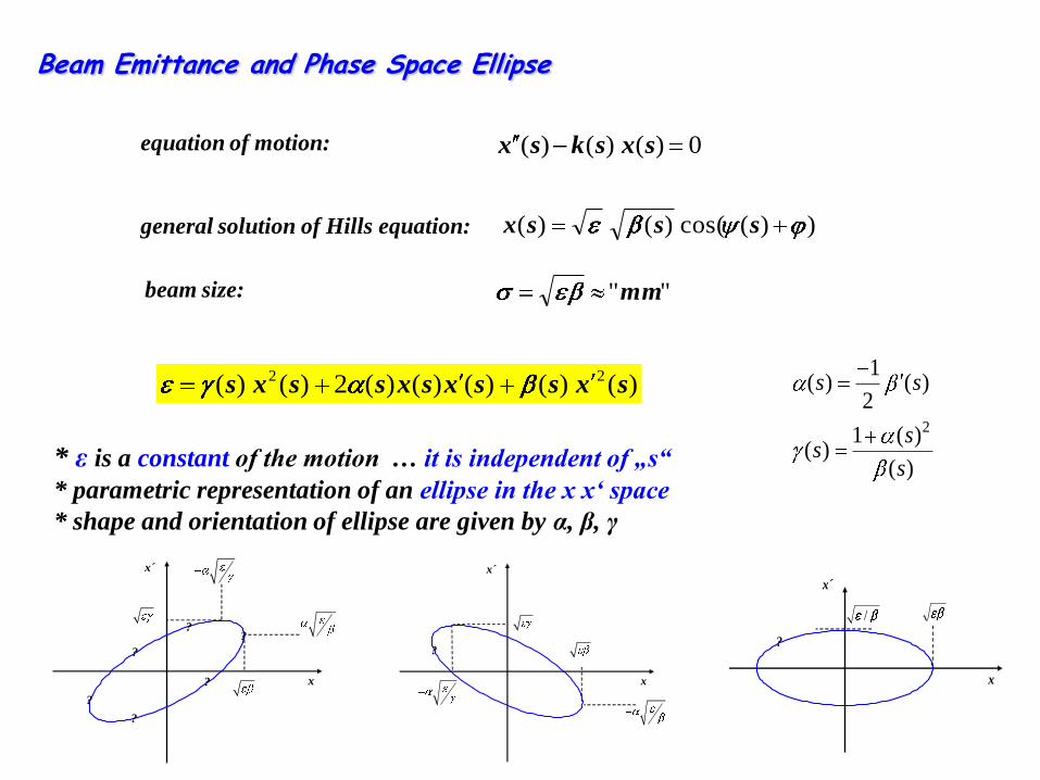
general solution of Hills equation:

* ε is a constant of the motion … it is independent of „s“

* parametric representation of an ellipse in the x x‘ space

* shape and orientation of ellipse are given by α, β, γ

equation of motion:

2

1( ) ( )

2

1 ( )( )

( )

s s

ss

s

""mmbeam size:

0)()()( sxsksx

))(cos()()( sssx

x´

x

?

?

?

?

?

?

x´

x

?

x´

x

?

/

)()()()()(2)()( 22sxssxsxssxs

Beam Emittance and Phase Space Ellipse

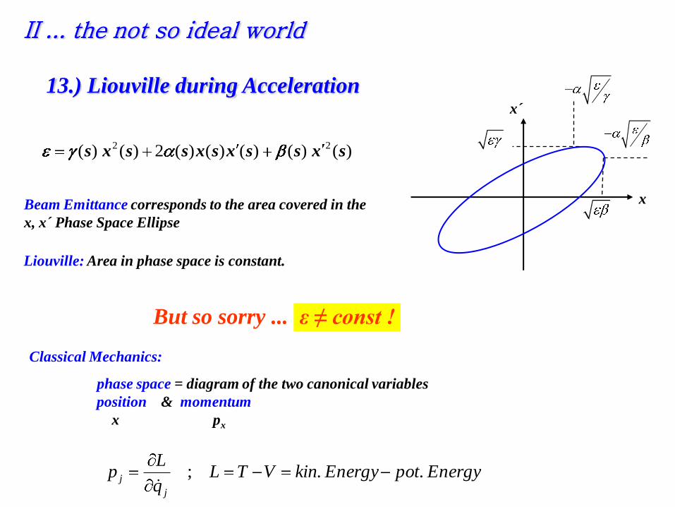
13.) Liouville during Accelerationx´

xBeam Emittance corresponds to the area covered in the

x, x´ Phase Space Ellipse

Liouville: Area in phase space is constant.

But so sorry ... ε ≠ const !

Classical Mechanics:

phase space = diagram of the two canonical variables

position & momentum

x px

EnergypotEnergykinVTLq

Lp

j

j ..;

)()()()()(2)()( 22sxssxsxssxs

II ... the not so ideal world

According to Hamiltonian mechanics:

phase space diagram relates the variables q and p

Liouvilles Theorem: p dq const

for convenience (i.e. because we are lazy bones) we use in accelerator theory:

xdx dx dtx

ds dt dswhere βx= vx / c

1x dx

the beam emittance

shrinks during

acceleration ε ~ 1 / γ

q = position = x

p = momentum = γmv = mcγβx

2

2

1

1

c

v c

xx

;

dxmcpdq x

dxxmcpdq

ε

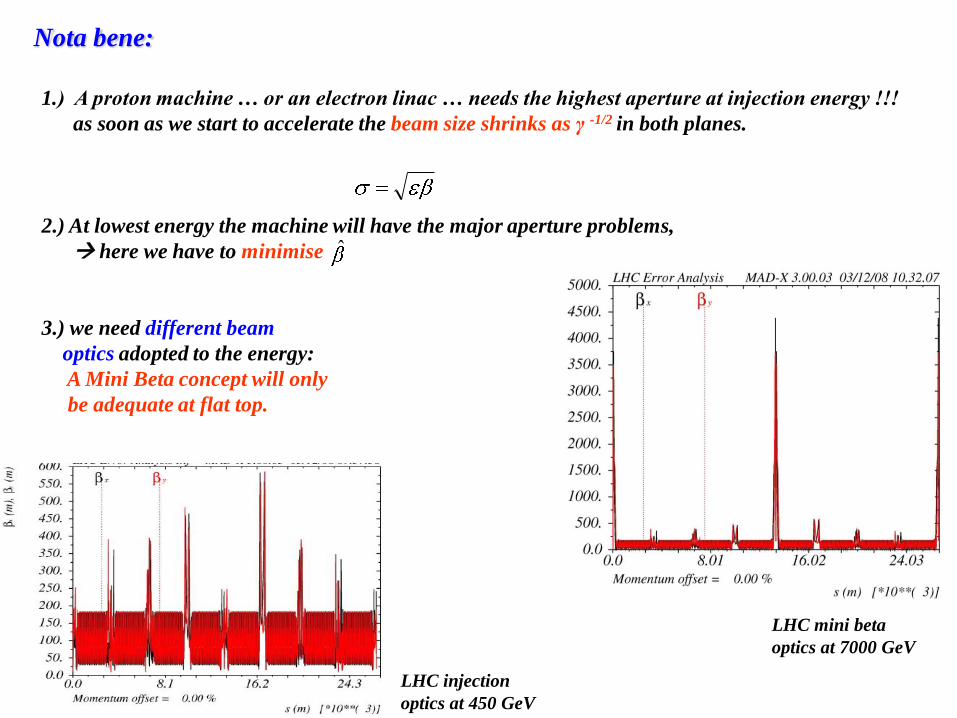
Nota bene:

1.) A proton machine … or an electron linac … needs the highest aperture at injection energy !!!

as soon as we start to accelerate the beam size shrinks as γ -1/2 in both planes.

2.) At lowest energy the machine will have the major aperture problems,

here we have to minimise

3.) we need different beam

optics adopted to the energy:

A Mini Beta concept will only

be adequate at flat top.

ˆ

LHC injection

optics at 450 GeV

LHC mini beta

optics at 7000 GeV

Example: HERA proton ring

injection energy: 40 GeV γ = 43

flat top energy: 920 GeV γ = 980

emittance ε (40GeV) = 1.2 * 10 -7

ε (920GeV) = 5.1 * 10 -9

7 σ beam envelope at E = 40 GeV

… and at E = 920 GeV

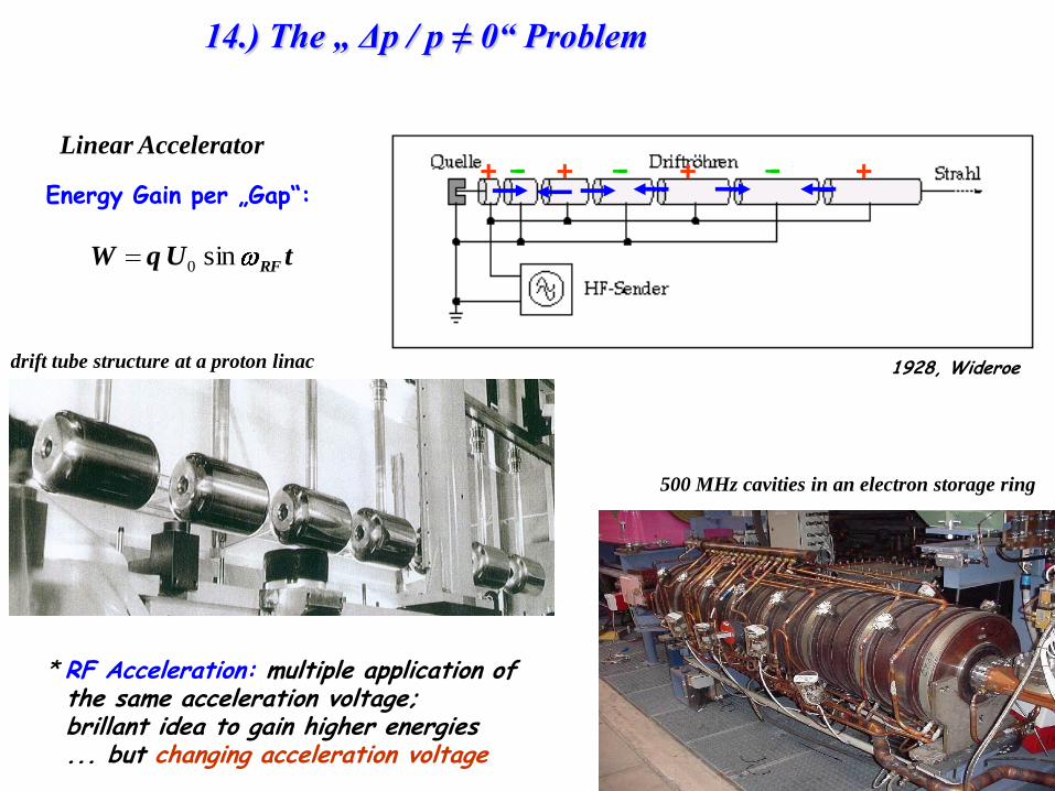
Linear Accelerator

1928, Wideroe

+ + + +- - -

* RF Acceleration: multiple application of the same acceleration voltage;brillant idea to gain higher energies ... but changing acceleration voltage

Energy Gain per „Gap“:

tUqW RFsin0

500 MHz cavities in an electron storage ring

drift tube structure at a proton linac

14.) The „ Δp / p ≠ 0“ Problem

Problem: panta rhei !!!(Heraklit: 540-480 v. Chr.)

Z X Y( )

Bunch length of Electrons ≈ 1cmExample: HERA RF:

U0

t c

MHz500cm60

cm60

994.0)84sin(

1)90sin(

o

o

3100.6U

U

typical momentum spread of an electron bunch: 3100.1

p

p

15.) Dispersion: trajectories for Δp / p ≠ 0

vBex

mvx

dt

dmF y

2

2

2

)( yρ

s

x

remember: x ≈ mm , ρ ≈ m … develop for small x

veBxmv

dt

xdm y)1(

2

2

2

consider only linear fields, and change independent variable: t → s

mv

gxe

mv

Bexx 0)1(

1

p=p0+Δp

Force acting on the particle

… but now take a small momentum error into account !!!

x

BxBB

y

y 0

y

Dispersion:

develop for small momentum error2

000

0

11

p

p

ppppp

10xk

2

00

02

00

0

2

1

p

pxeg

p

xegeB

p

p

p

Bexx

1

0

2p

pkx

xx

1)

1(

0

2p

pkxx

Momentum spread of the beam adds a term on the r.h.s. of the equation of motion.

inhomogeneous differential equation.

xkp

pxk

p

eB

p

pxx *

1**

)(*

00

0

0

2

1

2

1 1( )

px x k

p

general solution:

( ) ( ) ( )h ix s x s x s

( ) ( ) ( ) 0h hx s K s x s

1( ) ( ) ( )i i

px s K s x s

p

Normalise with respect to Δp/p:

( )( ) i

pp

x sD s

Dispersion function D(s)

* is that special orbit, an ideal particle would have for Δp/p = 1

* the orbit of any particle is the sum of the well known xβ and the dispersion

* as D(s) is just another orbit it will be subject to the focusing properties of the lattice

.ρ

xβ

Closed orbit for Δp/p > 0

( ) ( )i

px s D s

p

Matrix formalism:

( ) ( ) ( )p

x s x s D sp

0 0( ) ( ) ( ) ( )p

x s C s x S s x D sp

0s

x C S x Dp

x C S x Dp

DispersionExample: homogenous dipole field

00 0 1p p

p ps

x C S D x

x C S D x

Example HERA

3

1...2

( ) 1...2

1 10

x mm

D s m

pp

Amplitude of Orbit oscillation

contribution due to Dispersion ≈ beam size

Calculate D, D´

1 1

0 0

1 1( ) ( ) ( ) ( ) ( )

s s

s s

D s S s C s ds C s S s ds

D

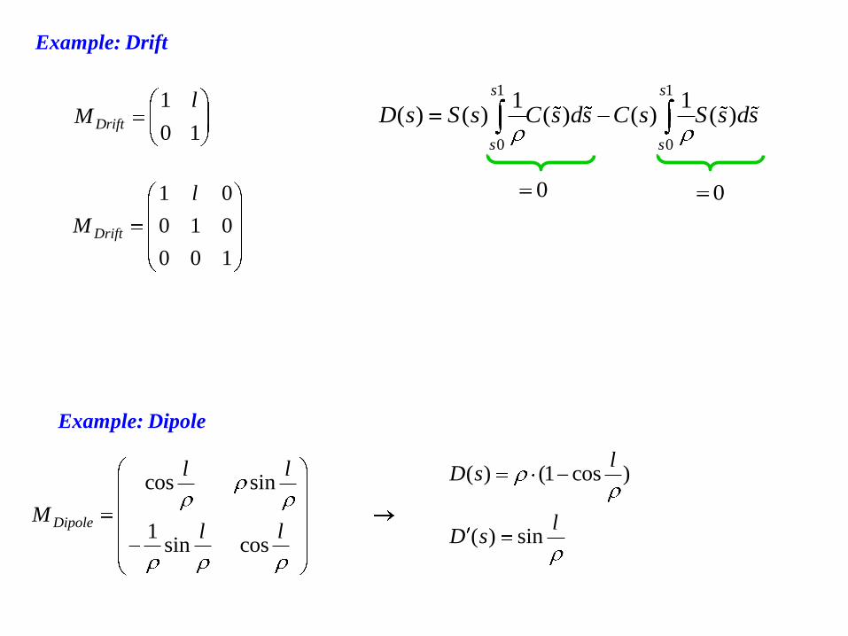
Example: Drift

1

0 1Drift

lM

1 0

0 1 0

0 0 1

Drift

l

M

1 1

0 0

1 1( ) ( ) ( ) ( ) ( )

s s

s s

D s S s C s ds C s S s ds

0 0

Example: Dipole

cos sin

1sin cos

Dipole

l l

Ml l

( ) (1 cos )

( ) sin

lD s

lD s

p

p*)s(Dx

D

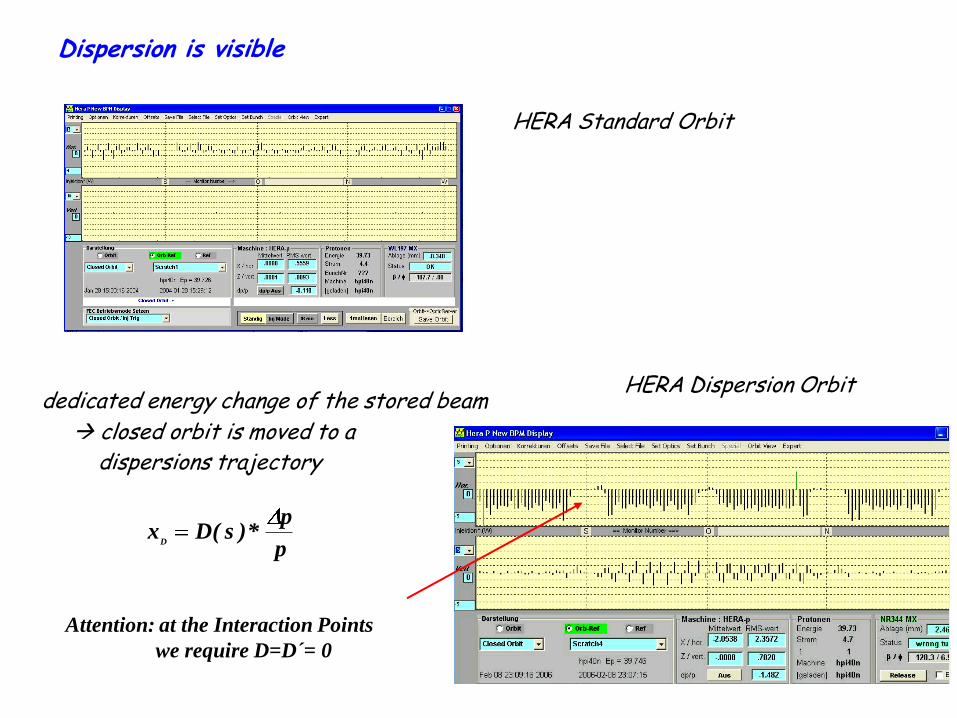
Dispersion is visible

HERA Standard Orbit

dedicated energy change of the stored beam

closed orbit is moved to a dispersions trajectory

HERA Dispersion Orbit

Attention: at the Interaction Points

we require D=D´= 0

16.) Momentum Compaction Factor:

The dispersion function relates the momentum error of a particle to the horizontal

orbit coordinate.

1( )*

px K s x

p

( ) ( ) ( )p

x s x s D sp

xβ

inhomogeneous differential equation

general solution

But it does much more:

it changes the length of the off - energy - orbit !!

ρ

ρ

dsx

dl

design orbit

particle trajectory

particle with a displacement x to the design orbit

path length dl ...

1( )

xdl ds

s

dl x

ds

1( )

EE

xl dl ds

s

circumference of an off-energy closed orbit

remember:

( ) ( )E

px s D s

p

( )

( )E

p D sl ds

p s

* The lengthening of the orbit for off-momentum

particles is given by the dispersion function

and the bending radius.

o

o

o

cp

l p

L p

1 ( )

( )cp

D sds

L s

For first estimates assume: 1

const

1 1 1 12cp dipolesl D D

L L

2cp

DD

L R

Assume: v c

cp

lT p

T L p

Definition:

αcp combines via the dispersion function

the momentum spread with the longitudinal

motion of the particle.

o

dipoledipoles

dipoles

DldssD *)()(

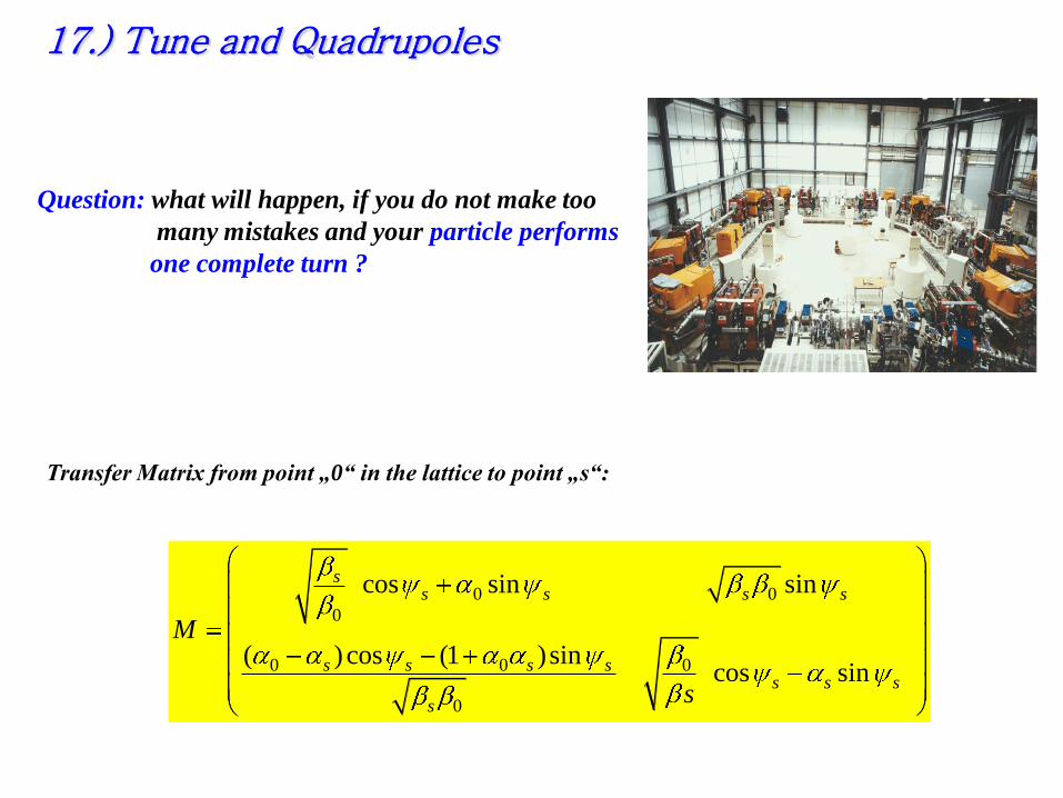
Question: what will happen, if you do not make too

many mistakes and your particle performs

one complete turn ?

17.) Tune and Quadrupoles

0 0

0

0 0 0

0

cos sin sin

( ) cos (1 )sincos sin

ss s s s

s s s ss s s

s

M

s

Transfer Matrix from point „0“ in the lattice to point „s“:

cos sin sin

sin cos sin

turn turn turnturn

turn turn turn

C SM

C S

Definition: phase advance

of the particle oscillation

per revolution in units of 2π

is called tune

2 2

turnQ

x(s)

s

0

Matrix for one complete turn

the Twiss parameters are periodic in L:( ) ( )

( ) ( )

( ) ( )

s L s

s L s

s L s

Quadrupole Error in the Lattice

optic perturbation described by thin lens quadrupole

0

rule for getting the tune

Quadrupole error Tune Shift

ideal storage ringquad error

turnturnturn

turnturnturn

kdistKds

MMMsincossin

sinsincos*

1

01* 0

turnturnturnturnturnturn

turnturnturn

distKdsKds

Msincossin*sin)sin(cos

sinsincos

00 sincos2cos2)( KdsMTrace

remember the old fashioned trigonometric stuff and assume that the error is small !!!

1

and referring to Q instead of ψ:

2

sincos)cos( 0

00

Kds

2

sincossin*sincos*cos 0

000

Kds

2

Kds

Q2

Ls

s

dsssKQ

0

04

)()(

a quadrupol error leads to a shift of the tune:

! the tune shift is proportional to the β-function at the quadrupole

!! field quality, power supply tolerances etc are much tighter at places where β is large

!!! mini beta quads: β ≈ 1900

arc quads: β ≈ 80

!!!! β is a measure for the sensitivity of the beam

Example: measurement of β in a storage ring:

GI06 NR

y = -6.7863x + 0.3883

y = -3E-12x + 0.28140.2800

0.2850

0.2900

0.2950

0.3000

0.3050

0.01250 0.01300 0.01350 0.01400 0.01450

k*L

Qx

,Qy

tune spectrum ... tune shift as a function of a gadient change

44

)()(0

0

quadLs

s

KldsssKQ

18.) Chromaticity:

A Quadrupole Error for Δp/p ≠ 0

Influence of external fields on the beam: prop. to magn. field & prop. zu 1/p

dipole magnet

focusing lensg

kp

e

particle having ...

to high energy

to low energy

ideal energy

ep

dlB

/ p

psDsxD )()(

definition of chromaticity:

gk

pe

Chromaticity: Q'

in case of a momentum spread:

… which acts like a quadrupole error in the machine and leads to a tune spread:

0p p p

kkgp

p

p

e

pp

egk 0

000

)1(

0

0

kp

pk

dsskp

pQ )(

4

10

0

p

pQQ '

Problem: chromaticity is generated by the lattice itself !!

ξ is a number indicating the size of the tune spot in the working diagram,

ξ is always created if the beam is focussed

it is determined by the focusing strength k of all quadrupoles

k = quadrupole strength

β = betafunction indicates the beam size … and even more the sensitivity of

the beam to external fields

Example: HERA

HERA-p: Q' = -70 … -80

Δ p/p = 0.5 *10-3

Q = 0.257 … 0.337

Some particles get very close to

resonances and are lost

odssskQ )()(*

4

1

dsssDkskQ )()()(4

121

N

Sextupole Magnets:

Correction of Q':

1.) sort the particles acording to their momentum ( ) ( )D

px s D s

p

2.) apply a magnetic field that rises quadratically with x (sextupole field)

xB gxz

2 21( )

2zB g x z

linear rising

„gradient“: x zB B

gxz x

S

SN

corrected chromaticity:

k1 normalised quadrupole strength

xkep

xgsextk *

/

~)( 21

p

pDksextk **)( 21

k2 normalised sextupole strength

D

x

D

xsext

D

sextD

F

x

F

xsext

F

sextF

x DlkDlkdssskQ 2214

1

4

1)()(*

4

1

Chromaticity in the FoDo Lattice

(1 sin )2ˆ

sin

L (1 sin )2

sin

Lβ-Function in a FoDo

x

y

dssskQ )()(*4

1

QfNQ

ˆ

*4

1

sin

)2

sin1()2

sin1(

*1

*4

1LL

fNQ

Q

remember ...

sin 2sin cos2 2

x xx

putting ...

sin2 4 Q

L

f

contribution of one FoDo Cell to the chromaticity of the ring:

using some TLC transformations ... ξ can be expressed in a very simple form:

sin

2sin2

*1

*4

1L

fNQ

Q

2cos

2sin

2sin

*1

*4

1L

fNQ

Q

2sin

2tan

*4

1L

fQ

Q

cell

2tan*

1cellQ

question: main contribution to ξ in a lattice … ?

Chromaticity

interaction region

odsssKQ )()(

4

1

19.) Resume´:1

beam emittance:

2

0 0 0( ) 2s s s

2

0

0

( )s

s

beta function in a drift:

… and for α = 0

1)

1(

0

2p

pkxxparticle trajectory for Δp/p ≠ 0

inhomogenious equation:

( ) ( ) ( )p

x s x s D sp

… and its solution:

momentum compaction: p

p

L

lcp

R

DD

Lcp

2

quadrupole error:

chromaticity:

ls

s

dsssKQ

0

04

)()(

dsssKQ )()(4

1