introduction to the equations of fluid dynamics and the

1

Introduction to the equations offluid dynamics and the finite

element approximation

1.1 General remarks and classification of fluid dynamicsproblems discussed in this book

The problems of solid and fluid behaviour are in many respects similar. In both mediastresses occur and in both the material is displaced. There is, however, one majordifference. Fluids cannot support any deviatoric stresses when at rest. Thus only apressure or a mean compressive stress can be carried. As we know, in solids deviatoricstresses can exist and a solid material can support general forms of structural forces.

In addition to pressure, deviatoric stresses can develop when the fluid is in motion andsuch motion of the fluid will always be of primary interest in fluid dynamics. We shalltherefore concentrate on problems in which displacement is continuously changing andin which velocity is the main characteristic of the flow. The deviatoric stresses whichcan now occur will be characterized by a quantity that has great resemblance to theshear modulus of solid mechanics and which is known as dynamic viscosity (molecularviscosity).

Up to this point the equations governing fluid flow and solid mechanics appear tobe similar with the velocity vector u replacing the displacement which often uses thesame symbol. However, there is one further difference, even when the flow has aconstant velocity (steady state), convective acceleration effects add terms which makethe fluid dynamics equations non-self-adjoint. Therefore, in most cases, unless thevelocities are very small so that the convective acceleration is negligible, the treatmenthas to be somewhat different from that of solid mechanics. The reader should notethat for self-adjoint forms, approximating the equations by the Galerkin method givesthe minimum error in the energy norm and thus such approximations are in a senseoptimal. In general, this is no longer true in fluid mechanics, though for slow flows(creeping flows) where the convective acceleration terms are negligible the situation issomewhat similar.

With a fluid which is in motion, conservation of mass is always necessary and, unlessthe fluid is highly compressible, we require that the divergence of the velocity vectorbe zero. Similar problems are encountered in the context of incompressible elasticity

2 Introduction to the equations of fluid dynamics and the finite element approximation

and the incompressibility constraint can introduce difficulties in the formulation (viz.reference 1). In fluid mechanics the same difficulty again arises and all fluid mechanicsapproximations have to be such that, even if compressibility is possible, the limit ofincompressibility can be modelled. This precludes the use of many elements whichare otherwise acceptable.

In this book we shall introduce the reader to finite element treatment of the equa-tions of motion for various problems of fluid mechanics. Much of the activity in fluidmechanics has, however, pursued a finite difference formulation and more recently aderivative of this known as the finite volume technique. Competition between finiteelement methods and techniques of finite differences have appeared and led to a muchslower adoption of the finite element process in fluid dynamics than in structures. Thereasons for this are perhaps simple. In solid mechanics or structural problems, the treat-ment of continua often arises in combination with other structural forms, e.g. trusses,beams, plates and shells. The engineer often dealing with structures composed ofstructural elements does not need to solve continuum problems. In addition when con-tinuum problems are encountered, the system can lead to use of many different materialmodels which are easily treated using a finite element formulation. In fluid mechanics,practically all situations of flow require a two- or three-dimensional treatment and hereapproximation is required. This accounts for the early use of finite differences in the1950s before the finite element process was made available. However, as pointed outin reference 1, there are many advantages of using the finite element process. This notonly allows a fully unstructured and arbitrary domain subdivision to be used but alsoprovides an approximation which in self-adjoint problems is always superior to or atleast equal to that provided by finite differences.

A methodology which appears to have gained an intermediate position is that offinite volumes, which were initially derived as a subclass of finite difference methods.As shown later in this chapter, these are simply another kind of finite element formin which subdomain collocation is used. We do not see much advantage in using thisform of approximation; however, there is one point which seems to appeal to someinvestigators. That is the fact the finite volume approximation satisfies conservationconditions for each finite volume. This does not carry over to the full finite elementanalysis where generally satisfaction of conservation conditions is achieved only in anassembly region of elements surrounding each node. Satisfaction of the conservationconditions on an individual element is not an advantage if the general finite elementapproximation gives results which are superior.

In this book we will discuss various classes of problems, each of which has a certainbehaviour in the numerical solution. Here we start with incompressible flows or flowswhere the only change of volume is elastic and associated with transient changes ofpressure (Chapters 4 and 5). For such flows full incompressible constraints must beavailable.

Further, with very slow speeds, convective acceleration effects are often negligibleand the solution can on occasion be reached using identical programs to those derivedfor linear incompressible elasticity. This indeed was the first venture of finite elementdevelopers into the field of fluid mechanics thus transferring the direct knowledge fromsolid mechanics to fluids. In particular the so-called linear Stokes flow is the case wherefully incompressible but elastic behaviour occurs. A particular variant of Stokes flow isthat used in metal forming where the material can no longer be described by a constant

General remarks for fluid mechanics problems 3

viscosity but possesses a viscosity which is non-Newtonian and depends on the strainrates. Chapter 5 is partly devoted to such problems. Here the fluid formulation (flowformulation) can be applied directly to problems such as the forming of metals orplastics and we shall discuss this extreme situation in Chapter 5. However, even inincompressible flows, when the speed increases convective acceleration terms becomeimportant. Here often steady-state solutions do not exist or at least are extremelyunstable. This leads us to such problems as vortex shedding. Vortex shedding indicatesthe start of instability which becomes very irregular and indeed random when high speedflow occurs in viscous fluids. This introduces the subject of turbulence, which occursfrequently in fluid dynamics. In turbulent flows random fluctuation of velocity occursat all points and the problem is highly time dependent. With such turbulent motion, itis possible to obtain an averaged solution using time averaged equations. Details ofsome available time averaged models are summarized in Chapter 8.

Chapter 6 deals with incompressible flow in which free surface and other gravity con-trolled effects occur. In particular we show three different approaches for dealing withfree surface flows and explain the necessary modifications to the general formulation.

The next area of fluid dynamics to which much practical interest is devoted is ofcourse that of flow of gases for which the compressibility effects are much larger. Herecompressibility is problem dependent and generally obeys gas laws which relate thepressure to temperature and density. It is now necessary to add the energy conservationequation to the system governing the motion so that the temperature can be evaluated.Such an energy equation can of course be written for incompressible flows but thisshows only a weak or no coupling with the dynamics of the flow. This is not the casein compressible flows where coupling between all equations is very strong. In suchcompressible flows the flow speed may exceed the speed of sound and this may lead toshock development. This subject is of major importance in the field of aerodynamicsand we shall devote a part of Chapter 7 to this particular problem.

In a real fluid, viscosity is always present but at high speeds such viscous effects areconfined to a narrow zone in the vicinity of solid boundaries (the so-called boundarylayer). In such cases, the remainder of the fluid can be considered to be inviscid. Therewe can return to the fiction of an ideal fluid in which viscosity is not present and herevarious simplifications are again possible. Such simplifications have been used sincethe early days of aerodynamics and date back to the work of Prandtl and Schlichting.2

One simplification is the introduction of potential flow and we shall mention this laterin this chapter. Potential flows are indeed the topic of many finite element investigators,but unfortunately such solutions are not easily extendible to realistic problems.

A particular form of viscous flow problem occurs in the modelling of flow in porousmedia. This important field is discussed in Chapter 9. In the topic of flow throughporous media, two extreme situations are often encountered. In the first, the porousmedium is stationary and the fluid flow occurs only in the narrow passages between solidgrains. Such an extreme is the basis of porous medium flow modelling in applicationssuch as geo-fluid dynamics where the flow of water or oil through porous rocks occurs.The other extreme of porous media flow is the one in which the solid occupies only asmall part of the total volume (for example, representing thermal insulation systems,heat exchangers etc.). In such problems flow is almost the same as that occurring influids without the solid phase which only applies an added, distributed, resistance toflow. Both extremes are discussed in Chapter 9.


Another major field of fluid mechanics of interest to us is that of shallow waterflows that occur in coastal estuaries or elsewhere. In this class of problems the depthdimension of flow is very much less than the horizontal ones. Chapter 10 will dealwith such problems in which essentially the distribution of pressure in the verticaldirection is almost hydrostatic. For such shallow water problems a free surface alsooccurs and this dominates the flow characteristics and here we note that shallow waterflow problems result in a formulation which is closely related to gas flow.

Whenever a free surface occurs it is possible for transient phenomena to happen,generating waves such as those occurring in oceans or other bodies of water. We haveintroduced in this book two chapters (Chapters 11 and 12) dealing with this particularaspect of fluid dynamics. Such wave phenomena are also typical of some other physicalproblems. For instance, acoustic and electromagnetic waves can be solved using similarapproaches. Indeed, one can show that the treatment for this class of problems is verysimilar to that of surface wave problems.

In what remains of this chapter we shall introduce the general equations of fluiddynamics valid for most compressible or incompressible flows showing how the par-ticular simplification occurs in some categories of problems mentioned above. How-ever, before proceeding with the recommended discretization procedures, which wepresent in Chapter 3, we must introduce the treatment of problems in which convectionand diffusion occur simultaneously. This we shall do in Chapter 2 using the scalarconvection–diffusion–reaction equation. Based on concepts given in Chapter 2, Chap-ter 3 will introduce a general algorithm capable of solving most of the fluid mechanicsproblems encountered in this book. There are many possible algorithms and very oftenspecialized ones are used in different areas of applications. However, the general algo-rithm of Chapter 3 produces results which are at least as good as others achieved bymore specialized means. We feel that this will give a certain unification to the wholesubject of fluid dynamics and, without apology, we will omit reference to many othermethods or discuss them only in passing.

For completeness we shall show in the present chapter some detail of the finiteelement process to avoid the repetition of basic finite element presentations which weassume are known to the reader either from reference 1 or from any of the numeroustexts available.

1.2 The governing equations of fluid dynamics3−9

1.2.1 Stresses in fluids

As noted above, the essential characteristic of a fluid is its inability to sustain deviatoricstresses when at rest. Here only hydrostatic ‘stress’or pressure is possible. Any analysismust therefore concentrate on the motion, and the essential independent variable is thevelocity u or, if we adopt indicial notation (with the coordinate axes referred to asxi, i = 1, 2, 3),

ui, i = 1, 2, 3 or u = [u1, u2, u3

]T(1.1)

This replaces the displacement variable which is of primary importance in solidmechanics.

The governing equations of fluid dynamics 5

The rates of strain are the primary cause of the general stresses, σij , and these aredefined in a manner analogous to that of infinitesimal strain in solid mechanics as

εij = 1

2

(∂ui

∂xj

+ ∂uj

∂xi

)(1.2)

This is a well-known tensorial definition of strain rates but for use later in variationalforms is written as a vector which is more convenient in finite element analysis. Detailsof such matrix forms are given fully in reference 1 but for completeness we summarizethem here. Thus, the strain rate is written as a vector (ε) and is given by the followingform

ε = [ε11, ε22, 2ε12]T = [ε11, ε22, γ12]T (1.3a)

in two dimensions with a similar form in three dimensions

ε = [ε11, ε22, ε33, 2ε12, 2ε23, 2ε31]T (1.3b)

When such vector forms are used we can write the strain rate vector in the form

ε = Su (1.4)

where S is known as the strain rate operator and u is the velocity given in Eq. (1.1).The stress–strain rate relations for a linear (Newtonian) isotropic fluid require the

definition of two constants. The first of these links the deviatoric stresses τij to thedeviatoric strain rates:

τij ≡ σij − 13δij σkk = 2µ

(εij − 1

3δij εkk

)(1.5)

In the above equation the quantity in brackets is known as the deviatoric strain rate,δij is the Kronecker delta, and a repeated index implies summation over the range ofthe index; thus

σkk ≡ σ11 + σ22 + σ33 and εkk ≡ ε11 + ε22 + ε33 (1.6)

The coefficient µ is known as the dynamic (shear) viscosity or simply viscosity andis analogous to the shear modulus G in linear elasticity.

The second relation is that between the mean stress changes and the volumetric strainrate. This defines the pressure as

p = − 13 σkk = −κ εkk + p0 (1.7)

where κ is a volumetric viscosity coefficient analogous to the bulk modulus K in linearelasticity and p0 is the initial hydrostatic pressure independent of the strain rate (notethat p and p0 are invariably defined as positive when compressive).

We can immediately write the ‘constitutive’ relation for fluids from Eqs (1.5) and(1.7)

σij = τij − δij p

= 2µ(εij − 1

3δij εkk

)+ κ δij εkk − δijp0

(1.8a)


or

σij = 2µεij + δij (κ− 23 µ) εkk − δij p0 (1.8b)

The Lame notation is occasionally used, putting

κ− 23 µ ≡ λ (1.9)

but this has little to recommend it and the relation (1.8a) is basic.There is little evidence about the existence of volumetric viscosity and, in what

follows, we shall takeκ εkk ≡ 0 (1.10)

giving the essential constitutive relation as (now dropping the suffix on p0)

σij = 2µ(εij − 1

3 δij εkk

)− δij p ≡ τij − δij p (1.11a)

without necessarily implying incompressibility εkk = 0. In the above,

τij = 2µ(εij − 1

3 δij εkk

)= µ

[(∂ui

∂xj

+ ∂uj

∂xi

)− 2

3δij

∂uk

∂xk

](1.11b)

The above relationships are identical to those of isotropic linear elasticity as wewill note again later for incompressible flow. However, in solid mechanics we oftenconsider anisotropic materials where a larger number of parameters (i.e. more than 2) arerequired to define the stress–strain relations. In fluid mechanics use of such anisotropyis rare and in this book we will limit ourselves to purely isotropic behaviour.

Non-linearity of some fluid flows is observed with a coefficientµ depending on strainrates. We shall term such flows ‘non-Newtonian’.

We now consider the basic conservation principles used to write the equations offluid dynamics. These are: mass conservation, momentum conservation and energyconservation.

1.2.2 Mass conservation

If ρ is the fluid density then the balance of mass flow ρui entering and leaving aninfinitesimal control volume (Fig. 1.1) is equal to the rate of change in density asexpressed by the relation

∂ρ

∂t+ ∂

∂xi

(ρui) ≡ ∂ρ

∂t+ ∇T (ρu) = 0 (1.12)

where ∇T = [∂/∂x1, ∂/∂x2, ∂/∂x3

]is known as the gradient operator.

It should be noted that in this section, and indeed in all subsequent ones, the controlvolume remains fixed in space. This is known as the ‘Eulerian form’and displacementsof a particle are ignored. This is in contrast to the usual treatment in solid mechanicswhere displacement is a primary dependent variable.


It is possible to recast the above equations in relation to a moving frame of referenceand, if the motion follows the particle, the equations will be named ‘Lagrangian’.Such Lagrangian frame of reference is occasionally used in fluid dynamics and brieflydiscussed in Chapter 6.

1.2.3 Momentum conservation: dynamic equilibrium

In the j th direction the balance of linear momentum leaving and entering the controlvolume (Fig. 1.1) is to be in dynamic equilibrium with the stresses σij and body forcesρgj . This gives a typical component equation

∂(ρuj )

∂t+ ∂

∂xi

[(ρuj )ui] − ∂

∂xi

(σij ) − ρgj = 0 (1.13)

or using Eq. (1.11a),

∂(ρuj )

∂t+ ∂

∂xi

[(ρuj )ui] − ∂τij

∂xi

+ ∂p

∂xj

− ρgj = 0 (1.14)

with Eq. (1.11b) implied.The conservation of angular momentum merely requires the stress to be symmetric,

i.e.σij = σji or τij = τji

In the sequel we will use the term momentum conservation to imply both linear andangular forms.

1.2.4 Energy conservation and equation of state

We note that in the equations of Secs 1.2.2 and 1.2.3 the dependent variables are ui (thevelocity components), p (the pressure) and ρ (the density). The deviatoric stresses,

dx3

x2; (y)

dx2

dx1x1; (x)

x3; (z)

Fig. 1.1 Coordinate direction and the infinitesimal control volume.


of course, are defined by Eq. (1.11b) in terms of velocities and hence are dependentvariables.

Obviously, there is one variable too many for this equation system to be capable ofsolution. However, if the density is assumed constant (as in incompressible fluids) or ifa single relationship linking pressure and density can be established (as in isothermalflow with small compressibility) the system becomes complete and solvable.

More generally, the pressure (p), density (ρ) and absolute temperature (T ) are relatedby an equation of state of the form

ρ = ρ(p, T ) (1.15a)

For an ideal gas this takes the form

ρ = p

RT(1.15b)

where R is the universal gas constant.In such a general case, it is necessary to supplement the governing equation system by

the equation of energy conservation. This equation is of interest even if it is not coupledwith the mass and momentum conservation, as it provides additional information aboutthe behaviour of the system.

Before proceeding with the derivation of the energy conservation equation we mustdefine some further quantities. Thus we introduce e, the intrinsic energy per unit mass.This is dependent on the state of the fluid, i.e. its pressure and temperature or

e = e(T , p) (1.16)

The total energy per unit mass, E, includes of course the kinetic energy per unitmass and thus

E = e + 12 uiui (1.17)

Finally, we can define the enthalpy as

h = e + p

ρor H = h + 1

2 uiui = E + p

ρ(1.18)

and these variables are found to be convenient to express the conservation of energyrelation.

Energy transfer can take place by convection and by conduction (radiation generallybeing confined to boundaries). The conductive heat flux qi for an isotropic material isdefined as

qi = −k∂T

∂xi

(1.19)

where k is thermal conductivity.To complete the relationship it is necessary to determine heat source terms. These can

be specified per unit volume as qH due to chemical reaction (if any) and must includethe energy dissipation due to internal stresses, i.e. using Eqs (1.11a) and (1.11b),

∂

∂xi

(σij uj ) = ∂

∂xi

(τij uj ) − ∂

∂xj

(puj ) (1.20)


The balance of energy in a infinitesimal control volume can now be written as

∂(ρE)

∂t+ ∂

∂xi

(ρuiE) − ∂

∂xi

(k∂T

∂xi

)+ ∂

∂xi

(pui) − ∂

∂xi

(τij uj ) − ρgiui − qH = 0

(1.21a)

or more simply

∂(ρE)

∂t+ ∂

∂xi

(ρuiH) − ∂

∂xi

(k∂T

∂xi

)− ∂

∂xi

(τij uj ) − ρgiui − qH = 0

(1.21b)

Here, the penultimate term represents the rate of work done by body forces.

1.2.5 Boundary conditions

On the boundary of a typical fluid dynamics problem boundary conditions need to bespecified to make the solution unique. These are given simply as:

(a) The velocities can be described as

ui = ui on �u (1.22a)

or traction asti = njσij = ti on �t (1.22b)

where �u

⋃�t = �. Generally traction is resolved into normal and tangential

components to the boundary.(b) In problems for which consideration of energy is important the temperature on the

boundary is expressed asT = T on �T (1.23a)

or thermal flux

qn = −nik∂T

∂xi

= −k∂T

∂n= qn on �q (1.23b)

where �T

⋃�q = �.

(c) For problems of compressible flow the density is specified as

ρ = ρ on �ρ (1.24)

1.2.6 Navier--Stokes and Euler equations

The governing equations derived in the preceding sections can be written in a generalconservative form as

∂Φ∂t

+ ∂Fi

∂xi

+ ∂Gi

∂xi

+ Q = 0 (1.25)

in which Eq. (1.12), (1.14) or (1.21b) provides the particular entries to the vectors.


Thus, using indicial notation the vector of independent unknowns is

Φ =

⎧⎪⎪⎪⎪⎪⎨⎪⎪⎪⎪⎪⎩

ρ

ρu1

ρu2

ρu3

ρE

⎫⎪⎪⎪⎪⎪⎬⎪⎪⎪⎪⎪⎭

, (1.26a)

the convective flux is expressed as

Fi =

⎧⎪⎪⎪⎨⎪⎪⎪⎩

ρui

ρu1ui + pδ1i

ρu2ui + pδ2i

ρu3ui + pδ3i

ρHui

⎫⎪⎪⎪⎬⎪⎪⎪⎭

, (1.26b)

similarly, the diffusive flux is expressed as

Gi =

⎧⎪⎪⎪⎪⎪⎨⎪⎪⎪⎪⎪⎩

0−τ1i

−τ2i

−τ3i

−(τij uj ) − k∂T

∂xi

⎫⎪⎪⎪⎪⎪⎬⎪⎪⎪⎪⎪⎭

(1.26c)

and the source terms as

Q =

⎧⎪⎪⎪⎨⎪⎪⎪⎩

0ρg1

ρg2

ρg3

ρgiui − qH

⎫⎪⎪⎪⎬⎪⎪⎪⎭

(1.26d)

with

τij = µ[(∂ui

∂xj

+ ∂uj

∂xi

)− 2

3δij

∂uk

∂xk

]

The complete set of Eq. (1.25) is known as the Navier–Stokes equation. A particularcase when viscosity is assumed to be zero and no heat conduction exists is known asthe ‘Euler equation’ (where τij = 0 and qi = 0).

The above equations are the basis from which all fluid mechanics studies start andit is not surprising that many alternative forms are given in the literature obtained bycombinations of the various equations.5 The above set is, however, convenient andphysically meaningful, defining the conservation of important quantities. It should benoted that only equations written in conservation form will yield the correct, physicallymeaningful, results in problems where shock discontinuities are present.

In Appendix A, we show a particular set of non-conservative equations which arefrequently used. The reader is cautioned not to extend the use of non-conservativeequations to problems of high speed flow.

Inviscid, incompressible flow 11

In many actual situations one or another feature of the flow is predominant. Forinstance, frequently the viscosity is only of importance close to the boundaries atwhich velocities are specified. In such cases the problem can be considered separatelyin two parts: one as a boundary layer near such boundaries and another as inviscid flowoutside the boundary layer.

Further, in many cases a steady-state solution is not available with the fluid exhibit-ing turbulence, i.e. a random fluctuation of velocity. Here it is still possible to usethe general Navier–Stokes equations now written in terms of the mean flow with anadditional Reynolds stress term. Turbulent instability is inherent in the Navier–Stokesequations. It is in principle always possible to obtain the transient, turbulent, solutionmodelling of the flow, providing the mesh size is capable of reproducing the smalleddies which develop in the problem. Such computations are extremely costly andoften not possible at high Reynolds numbers. Hence the Reynolds averaging approachis of practical importance.

Two further points have to be made concerning inviscid flow (ideal fluid flow as it issometimes known). First, the Euler equations are of a purely convective form:

∂Φ∂t

+ ∂Fi

∂xi

+ Q = 0 Fi = Fi (Φ) (1.27)

and hence very special methods for their solutions will be necessary. These methodsare applicable and useful mainly in compressible flow, as we shall discuss in Chap-ter 7. Second, for incompressible (or nearly incompressible) flows it is of interest tointroduce a potential that converts the Euler equations to a simple self-adjoint form.We shall discuss this potential approximation in Sec. 1.3. Although potential forms arealso applicable to compressible flows we shall not use them as they fail in complexsituations.

1.3 Inviscid, incompressible flow

In the absence of viscosity and compressibility, ρ is constant and Eq. (1.12) can bewritten as

∂ui

∂xi

= 0 (1.28)

and Eq. (1.14) as∂ui

∂t+ ∂

∂xj

(ujui) + 1

ρ

∂p

∂xi

− gi = 0 (1.29)

1.3.1 Velocity potential solution

The Euler equations given above are not convenient for numerical solution, and it is ofinterest to introduce a potential, φ, defining velocities as

u1 = − ∂φ

∂x1u2 = − ∂φ

∂x2u3 = − ∂φ

∂x3

or

ui = − ∂φ

∂xi

(1.30)


If such a potential exists then insertion of Eq. (1.30) into Eq. (1.28) gives a singlegoverning equation

∂2φ

∂xi∂xi

≡ ∇2φ = 0 (1.31)

which, with appropriate boundary conditions, can be readily solved. Equation (1.31) isa classical Laplacian equation. For contained flow we can of course impose the normalvelocity un on the boundaries:

un = −∂φ∂n

= un (1.32)

and, as we shall see later, this provides a natural boundary condition for a weightedresidual or finite element solution.

Of course we must be assured that the potential function φ exists, and indeed deter-mine what conditions are necessary for its existence. Here we observe that so far inthe definition of the problem we have not used the momentum conservation equations(1.29), to which we shall now return. However, we first note that a single-valuedpotential function implies that

∂2φ

∂xj ∂xi

= ∂2φ

∂xi ∂xj

(1.33)

Defining vorticity as rotation rate per unit area

ωij = 1

2

(∂ui

∂xj

− ∂uj

∂xi

)(1.34)

we note that the use of the velocity potential in Eq. (1.34) gives

ωij = 0 (1.35)

and the flow is therefore named irrotational.Inserting the definition of potential into the first term of Eq. (1.29) and using

Eqs (1.28) and (1.34) we can rewrite Eq. (1.29) as

− ∂

∂xi

(∂φ∂t

)+ ∂

∂xi

[12ujuj + p

ρ+ P

]= 0 (1.36)

in which P is a potential of the body forces given by

gi = −∂P

∂xi

(1.37)

In problems involving constant gravity forces in the x2 direction the body force potentialis simply

P = g x2 (1.38)

Equation (1.36) is alternatively written as

∇(− ∂φ

∂t+ H + P

)= 0 (1.39)

Incompressible (or nearly incompressible) flows 13

where H is the enthalpy, given as H = uiui/2 + p/ρ.If isothermal conditions pertain, the specific energy is constant and Eq. (1.39) implies

that

−∂φ∂t

+ 1

2uiui + p

ρ+ P = constant (1.40)

over the whole domain. This can be taken as a corollary of the existence of the potentialand indeed is a condition for its existence. In steady-state flows it provides the well-known Bernoulli equation that allows the pressures to be determined throughout thewhole potential field once the value of the constant is established.

We note that the governing potential equation (1.31) is self-adjoint (see AppendixB) and that the introduction of the potential has side-stepped the difficulties of dealingwith convective terms. It is also of interest to note that the Laplacian equation, whichis obeyed by the velocity potential, occurs in other contexts. For instance, in two-dimensional flow it is convenient to introduce a stream function the contours of whichlie along the streamlines. The stream function, ψ, defines the velocities as

u1 = ∂ψ

∂x2and u2 = − ∂ψ

∂x1(1.41)

which satisfy the incompressibility condition (1.28)

∂ui

∂xi

= ∂

∂x1

(∂ψ

∂x2

)+ ∂

∂x1

(− ∂ψ

∂x1

)= 0 (1.42)

For an existence of a unique potential for irrotational flow we note that ω12 = 0[Eq. (1.34)] gives a Laplacian equation

∂2ψ

∂xi∂xi

= ∇2ψ = 0 (1.43)

The stream function is very useful in getting a pictorial representation of flow. InAppendix C we show how the stream function can be readily computed from a knowndistribution of velocities.

1.4 Incompressible (or nearly incompressible) flows

We observed earlier that the Navier–Stokes equations are completed by the existenceof a state relationship giving [Eq. (1.15a)]

ρ = ρ(p, T )

In (nearly) incompressible relations we shall frequently assume that:

(a) The problem is isothermal.(b) The variation of ρ with p is very small, i.e. such that in product terms of velocity

and density the latter can be assumed constant.

The first assumption will be relaxed, as we shall see later, allowing some thermalcoupling via the dependence of the fluid properties on temperature. In such cases we


shall introduce the coupling iteratively. For such cases the problem of density-inducedcurrents or temperature-dependent viscosity will be typical (see Chapters 5 and 6).

If the assumptions introduced above are used we can still allow for small com-pressibility, noting that density changes are, as a consequence of elastic deformability,related to pressure changes. Thus we can write

dρ = ρ

Kdp (1.44a)

where K is the elastic bulk modulus. This also can be written as

dρ = 1

c2dp (1.44b)

or

∂ρ

∂t= 1

c2

∂p

∂t(1.44c)

with c = √K/ρ being the acoustic wave velocity.

Equations (1.25) and (1.26a)–(1.26d) can now be rewritten omitting the energy trans-port equation (and condensing the general form) as

1

c2

∂p

∂t+ ρ

∂ui

∂xi

= 0 (1.45a)

∂uj

∂t+ ∂

∂xi

(ujui) + 1

ρ

∂p

∂xj

− 1

ρ

∂τji

∂xi

− gj = 0 (1.45b)

In three dimensions j = 1, 2, 3 and the above represents a system of four equations inwhich the variables are uj and p. Here

1

ρτij = ν

(∂ui

∂xj

+ ∂uj

∂xi

− 2

3δij

∂uk

∂xk

)where ν = µ/ρ is the kinematic viscosity.

The reader will note that the above equations, with the exception of the convectiveacceleration terms, are identical to those governing the problem of incompressible (orslightly compressible) elasticity (e.g. see Chapter 11 of reference 1).

1.5 Numerical solutions: weak forms, weighted residualand finite element approximation

1.5.1 Strong and weak forms

We assume the reader is already familiar with basic ideas of finite element and finitedifference methods. However, to avoid a constant cross-reference to other texts (e.g.reference 1), we provide here a brief introduction to weighted residual and finite elementmethods.

Numerical solutions: weak forms, weighted residual and finite element approximation 15

The Laplace equation, which we introduced in Sec. 1.3, is a very convenient examplefor the start of numerical approximations. We shall generalize slightly and discuss insome detail the quasi-harmonic (Poisson) equation

− ∂

∂xi

(k∂φ

∂xi

)+ Q = 0 (1.46)

where k and Q are specified functions. These equations together with appropriateboundary conditions define the problem uniquely. The boundary conditions can be ofDirichlet type

φ = φ on �φ (1.47a)

or that of Neumann type

qn = −k∂φ

∂n= qn on �q (1.47b)

where a bar denotes a specified quantity.Equations (1.46) to (1.47b) are known as the strong form of the problem.

Weak form of equationsWe note that direct use of Eq. (1.46) requires computation of second derivatives tosolve a problem using approximate techniques. This requirement may be weakenedby considering an integral expression for Eq. (1.46) written as∫

�

v

[− ∂

∂xi

(k∂φ

∂xi

)+ Q

]d� = 0 (1.48)

in which v is an arbitrary function. A proof that Eq. (1.48) is equivalent to Eq. (1.46)is simple.

If we assume Eq. (1.46) is not zero at some point xi in � then we can also let v bea positive parameter times the same value resulting in a positive result for the integralEq. (1.48). Since this violates the equality we conclude that Eq. (1.46) must be zerofor every xi in � hence proving its equality with Eq. (1.48).

We may integrate by parts the second derivative terms in Eq. (1.48) to obtain∫�

∂v

∂xi

(k∂φ

∂xi

)d� +

∫�

v Q d� −∫

�

v ni

(k∂φ

∂xi

)d� = 0 (1.49)

We now split the boundary into two parts, �φ and �q , with � = �φ

⋃�q , and use

Eq. (1.47b) in Eq. (1.49) to give∫�

∂v

∂xi

(k∂φ

∂xi

)d� +

∫�

v Q d� +∫

�q

v qn d� = 0 (1.50)

which is valid only if v vanishes on �φ. Hence we must impose Eq. (1.47a) forequivalence.

Equation (1.50) is known as the weak form of the problem since only first derivativesare necessary in constructing a solution. Such forms are the basis for the finite elementsolutions we use throughout this book.


Weighted residual approximationIn a weighted residual scheme an approximation to the independent variableφ is writtenas a sum of known trial functions (basis functions) Na(xi) and unknown parametersφa . Thus we can always write

φ ≈ φ = N1(xi)φ1 + N2(xi)φ

2 + · · ·

=n∑

a=1

Na(xi)φa = N(xi)φ

(1.51)

whereN = [N1, N2, · · · Nn

](1.52a)

andφ = [φ1, φ2, · · · φn

]T(1.52b)

In a similar way we can express the arbitrary variable v as

v ≈ v = W1(xi)v1 + W2(xi)v

2 + · · ·

=n∑

a=1

Wa(xi)va = W(xi)v

(1.53)

in which Wa are test functions and va arbitrary parameters. Using this form of approx-imation will convert Eq. (1.50) to a set of algebraic equations.

In the finite element method and indeed in all other numerical procedures for whicha computer-based solution can be used, the test and trial functions will generally bedefined in a local manner. It is convenient to consider each of the test and basis functionsto be defined in partitions �e of the total domain �. This division is denoted by

� ≈ �h =⋃

�e (1.54)

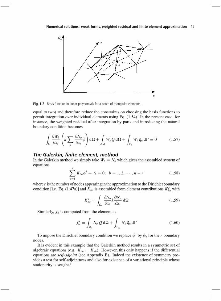
and in a finite element method �e are known as elements. The very simplest useslines in one dimension, triangles in two dimensions and tetrahedra in three dimensionsin which the basis functions are usually linear polynomials in each element and theunknown parameters are nodal values of φ. In Fig. 1.2 we show a typical set of suchlinear functions defined in two dimensions.

In a weighted residual procedure we first insert the approximate function φ into thegoverning differential equation creating a residual, R(xi), which of course should bezero at the exact solution. In the present case for the quasi-harmonic equation we obtain

R = − ∂

∂xi

(k∑

a

∂Na

∂xi

φa

)+ Q (1.55)

and we now seek the best values of the parameter set φa

which ensures that∫�

WbR d� = 0; b = 1, 2, · · · , n (1.56)

Note that this is the term multiplying the arbitrary parameter vb. As noted previously,integration by parts is used to avoid higher-order derivatives (i.e. those greater than or


Na

a

x

y

~

Fig. 1.2 Basis function in linear polynomials for a patch of trianglular elements.

equal to two) and therefore reduce the constraints on choosing the basis functions topermit integration over individual elements using Eq. (1.54). In the present case, forinstance, the weighted residual after integration by parts and introducing the naturalboundary condition becomes∫

�

∂Wb

∂xi

(k∑

a

∂Na

∂xi

φ

)d� +

∫�

WbQ d� +∫

�q

Wb qn d� = 0 (1.57)

The Galerkin, finite element, methodIn the Galerkin method we simply take Wb = Nb which gives the assembled system ofequations

n∑a=1

Kbaφa + fb = 0; b = 1, 2, · · · , n − r (1.58)

where r is the number of nodes appearing in the approximation to the Dirichlet boundarycondition [i.e. Eq. (1.47a)] and Kba is assembled from element contributions Ke

ba with

Keba =

∫�e

∂Nb

∂xi

k∂Na

∂xi

d� (1.59)

Similarly, fb is computed from the element as

f eb =

∫�e

Nb Q d� +∫

�eq

Nb qn d� (1.60)

To impose the Dirichlet boundary condition we replace φa by φa for the r boundarynodes.

It is evident in this example that the Galerkin method results in a symmetric set ofalgebraic equations (e.g. Kba = Kab). However, this only happens if the differentialequations are self-adjoint (see Appendix B). Indeed the existence of symmetry pro-vides a test for self-adjointness and also for existence of a variational principle whosestationarity is sought.1


(a) Three-node triangle. (b) Shape function for node 1.

y

1

3

x2

N1x2

x1

2

3

1

1

Fig. 1.3 Triangular element and shape function for node 1.

It is necessary to remark here that if we were considering a pure convection equation

ui

∂φ

∂xi

+ Q = 0 (1.61)

symmetry would not exist and such equations can often become unstable if the Galerkinmethod is used. We will discuss this matter further in the next chapter.

Example 1.1 Shape functions for triangle with three nodesA typical finite element with a triangular shape is defined by the local nodes 1, 2, 3 andstraight line boundaries between nodes as shown in Fig. 1.3(a) and will yield the shapeof Na of the form shown in Fig. 1.3(b). Writing a scalar variable as

φ = α1 + α2 x1 + α3 x2 (1.62)

we may evaluate the three constants by solving a set of three simultaneous equationswhich arise if the nodal coordinates are inserted and the scalar variable equated to theappropriate nodal values. For example, nodal values may be written as

φ1 = α1 + α2 x11 + α3 x1

2

φ2 = α1 + α2 x21 + α3 x2

2

φ3 = α1 + α2 x31 + α3 x3

2

(1.63)

We can easily solve for α1, α2 and α3 in terms of the nodal values φ1, φ2 and φ3 andobtain finally

φ = 1

2�

[(a1 + b1x1 + c1x2)φ

1 + (a2 + b2x1 + c2x2)φ2 + (a3 + b3x1 + c3x2)φ

3]

(1.64)

in whicha1 = x2

1x32 − x3

1x22

b1 = x22 − x3

2

c1 = x31 − x2

1

(1.65)


where xai is the i direction coordinate of node a and other coefficients are obtained by

cyclic permutation of the subscripts in the order 1, 2, 3, and

2� = det

∣∣∣∣∣∣1 x1

1 x12

1 x21 x2

2

1 x31 x3

2

∣∣∣∣∣∣ = 2 · (area of triangle 123) (1.66)

From Eq. (1.64) we see that the shape functions are given by

Na = (aa + ba x1 + ca x2)/(2�); a = 1, 2, 3 (1.67)

Since the unknown nodal quantities defined by these shape functions vary linearlyalong any side of a triangle the interpolation equation (1.64) guarantees continuitybetween adjacent elements and, with identical nodal values imposed, the same scalarvariable value will clearly exist along an interface between elements. We note, however,that in general the derivatives will not be continuous between element assemblies.1

Example 1.2 Poisson equation in two dimensions: Galerkinformulation with triangular elementsThe relations for a Galerkin finite elemlent solution have been given in Eqs (1.58)to (1.60). The components of Kba and fb can be evaluated for a typical element orsubdomain and the system of equations built by standard methods.

For instance, considering the set of nodes and elements shown shaded in Fig. 1.4(a),to compute the equation for node 1 in the assembled patch, it is only necessary tocompute the Ke

ba for two element shapes as indicated in Fig. 1.4(b). For the Type1 element [left element in Fig. 1.4(b)] the shape functions evaluated from Eq. (1.67)using Eqs (1.65) and (1.66) gives

N1 = 1 − x2

h; N2 = x1

h; N3 = x2 − x1

h

thus, the derivatives are given by:

∂N∂x1

=

⎧⎪⎪⎪⎪⎪⎨⎪⎪⎪⎪⎪⎩

∂N1

∂x1

∂N2

∂x1

∂N3

∂x1

⎫⎪⎪⎪⎪⎪⎬⎪⎪⎪⎪⎪⎭

=

⎧⎪⎪⎪⎪⎨⎪⎪⎪⎪⎩

0

1

h

−1

h

⎫⎪⎪⎪⎪⎬⎪⎪⎪⎪⎭

and∂N∂x2

=

⎧⎪⎪⎪⎪⎪⎨⎪⎪⎪⎪⎪⎩

∂N1

∂x2

∂N2

∂x2

∂N3

∂x2

⎫⎪⎪⎪⎪⎪⎬⎪⎪⎪⎪⎪⎭

=

⎧⎪⎪⎪⎪⎨⎪⎪⎪⎪⎩

−1

h

0

1

h

⎫⎪⎪⎪⎪⎬⎪⎪⎪⎪⎭

Similarly, for the Type 2 element [right element in Fig. 1.4(b)] the shape functionsare expressed by

N1 = 1 − x1

h; N2 = x1 − x2

h; N3 = x2

h


(a) ‘Connected’ equations for node 1.

(b) Type 1 and Type 2 element shapes in mesh.

h

5 4 3

6 1 2

7

3 2

1 12

3

8 9

h h

h

Fig. 1.4 Linear triangular elements for Poisson equation example.

and their derivatives by

∂N∂x1

=

⎧⎪⎪⎪⎪⎪⎨⎪⎪⎪⎪⎪⎩

∂N1

∂x1

∂N2

∂x1

∂N3

∂x1

⎫⎪⎪⎪⎪⎪⎬⎪⎪⎪⎪⎪⎭

=

⎧⎪⎪⎪⎪⎨⎪⎪⎪⎪⎩

−1

h1

h

0

⎫⎪⎪⎪⎪⎬⎪⎪⎪⎪⎭

and∂N∂x2

=

⎧⎪⎪⎪⎪⎪⎨⎪⎪⎪⎪⎪⎩

∂N1

∂x2

∂N2

∂x2

∂N3

∂x2

⎫⎪⎪⎪⎪⎪⎬⎪⎪⎪⎪⎪⎭

=

⎧⎪⎪⎪⎪⎨⎪⎪⎪⎪⎩

0

−1

h1

h

⎫⎪⎪⎪⎪⎬⎪⎪⎪⎪⎭

and

Evaluation of the matrix Keba and f e

b for Type 1 and Type 2 elements gives (refer toAppendix D for integration formulae)

Keφe = 1

2k

[1 0 −10 1 −1

−1 −1 2

] ⎧⎪⎨⎪⎩φ

1e

φ2e

φ3e

⎫⎪⎬⎪⎭

and

Keφe = 1

2k

[1 −1 0

−1 2 −10 −1 1

] ⎧⎪⎨⎪⎩φ

1e

φ2e

φ3e

⎫⎪⎬⎪⎭ ,


respectively. The force vector for a constant Q over each element is given by

f e = 1

6Q h2

{111

}

for both types of elements. Assembling the patch of elements shown in Fig. 1.4(b)gives the equation with non-zero coefficients for node 1 as (refer to references 1 and10 for assembly procedure)

k[4 −1 −1 −1 −1

]⎧⎪⎪⎪⎪⎪⎨⎪⎪⎪⎪⎪⎩

φ1

φ2

φ4

φ6

φ8

⎫⎪⎪⎪⎪⎪⎬⎪⎪⎪⎪⎪⎭

+ Q h2 = 0

Using a central difference finite difference approximation directly in the differentialequation (1.46) gives the approximation

k

h2

[4 −1 −1 −1 −1

]⎧⎪⎪⎪⎪⎪⎨⎪⎪⎪⎪⎪⎩

φ1

φ2

φ4

φ6

φ8

⎫⎪⎪⎪⎪⎪⎬⎪⎪⎪⎪⎪⎭

+ Q = 0

and we note that the assembled node using the finite element method is identical tothe finite difference approximation though presented slightly differently. If all theboundary conditions are forced (i.e. φ = φ) no differences arise between a finiteelement and a finite difference solution for the regular mesh assumed. However, ifany boundary conditions are of natural type or the mesh is irregular differences willarise, with the finite element solution generally giving superior answers. Indeed, norestrictions on shape of elements or assembly type are imposed by the finite elementapproach.

Example 1.3In Fig. 1.5 an example of a typical potential solution as described in Sec. 1.3 is given.Here we show the finite element mesh and streamlines for a domain of flow around asymmetric aerofoil.

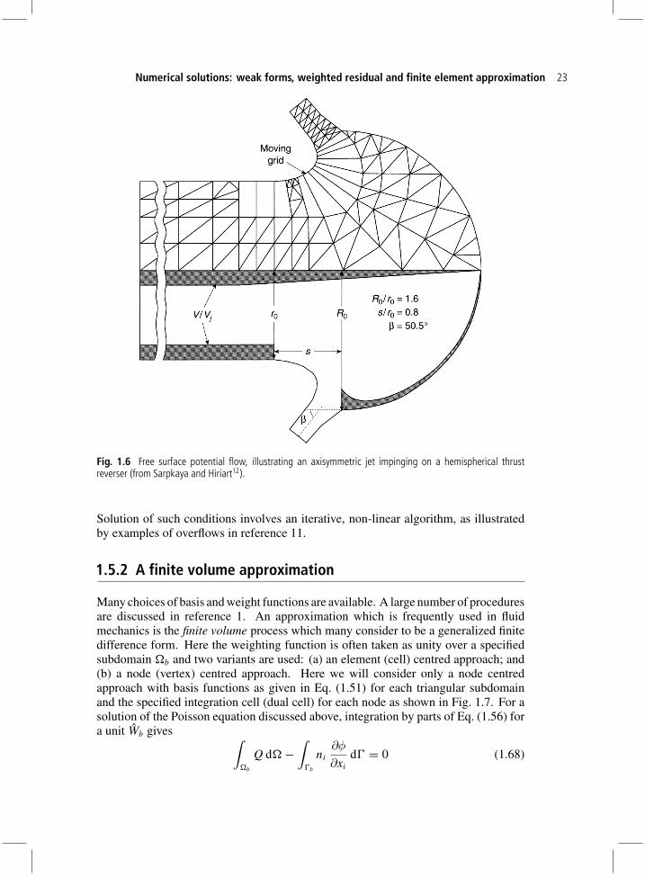
Example 1.4Some problems of specific interest are those of flow with a free surface.11,12,13 Herethe governing Laplace equation for the potential remains identical, but the free surfaceposition has to be found iteratively. In Fig. 1.6 an example of such a free surface flowsolution is given.12

For gravity forces given by Eq. (1.38) the free surface condition in two dimensions(x1, x2) requires

12 (u1u1 + u2u2) + gx2 = 0


Fig. 1.5 Potential flow solution around an aerofoil. Mesh and streamline plots.


Fig. 1.6 Free surface potential flow, illustrating an axisymmetric jet impinging on a hemispherical thrustreverser (from Sarpkaya and Hiriart12).

Solution of such conditions involves an iterative, non-linear algorithm, as illustratedby examples of overflows in reference 11.

1.5.2 A finite volume approximation

Many choices of basis and weight functions are available. A large number of proceduresare discussed in reference 1. An approximation which is frequently used in fluidmechanics is the finite volume process which many consider to be a generalized finitedifference form. Here the weighting function is often taken as unity over a specifiedsubdomain �b and two variants are used: (a) an element (cell) centred approach; and(b) a node (vertex) centred approach. Here we will consider only a node centredapproach with basis functions as given in Eq. (1.51) for each triangular subdomainand the specified integration cell (dual cell) for each node as shown in Fig. 1.7. For asolution of the Poisson equation discussed above, integration by parts of Eq. (1.56) fora unit Wb gives ∫

�b

Q d� −∫

�b

ni

∂φ

∂xi

d� = 0 (1.68)


Fig. 1.7 Finite volume weighting. Vertex centred method (�b).

for each subdomain �b with boundary �b. In this form the integral of the first termgives ∫

�b

Q d� = Q �b (1.69)

when Q is constant in the domain. Introduction of the basis functions into the secondterm gives ∫

�b

ni

∂φ

∂xi

d� ≈∫

�b

ni

∂φ

∂xi

d� =∫

�b

ni

∂Na

∂xi

d� φa

(1.70)

requiring now only boundary integrals of the shape functions. In order to make theprocess clearer we again consider the case for the patch of elements shown in Fig. 1.4(a).

Example 1.5 Poisson equation in two dimensions: finite vol-ume formulation with triangular elementsThe subdomain for the determination of equation for node 1 using the finite volumemethod is shown in Fig. 1.8(a). The shape functions and their derivatives for the Type 1and Type 2 elements shown in Fig. 1.8(b) are given in Example 1.2. We note especiallythat the derivatives of the shape functions in each element type are constant. Thus, theboundary integral terms in Eq. (1.70) become∫

�b

ni

∂Na

∂xi

d� =∑

e

∫�e

nei d�

∂Nea

∂xi

where e denotes the elements surrounding node a. Each of the integrals on �e will bean I1, I2, I3 for the Type 1 and Type 2 elements shown. It is simple to show that theintegral

I 11 =

∫�e

ne1 d� =

∫ c

4

ne1 d� +

∫ 6

c

ne1 d� = x6

2 − x42


5 4 3

7 8 9

6

1

2

(a) ‘Connected’ area for node 1.

3

6

c

4

1

5

2

I3 I2

I2I1

I3I1

6

1 24

3

5

c

(b) Type 1 and Type 2 element boundary integrals.

Fig. 1.8 Finite volume domain and integrations for vertex centred method.

where x42 , x6

2 are mid-edge coordinates of the triangle as shown in Fig. 1.8(b). Similarly,for the x2 derivative we obtain

I 21 =

∫�e

ne2 d� =

∫ c

4

ne2 d� +

∫ 6

c

ne2 d� = x4

1 − x61

Thus, the integral

I1 =∫

�e

ni

∂Na

∂xi

d� = ∂Na

∂x1(x6

2 − x42) + ∂Na

∂x2(x4

1 − x61)


The results I2 and I3 are likewise obtained as

I2 = ∂Na

∂x1(x4

2 − x52) + ∂Na

∂x2(x5

1 − x41)

I3 = ∂Na

∂x1(x5

2 − x62) + ∂Na

∂x2(x6

1 − x51)

Using the above we may write the finite volume result for the subdomain shown inFig. 1.8(a) as

k[4 −1 −1 −1 −1

]⎧⎪⎪⎪⎪⎪⎨⎪⎪⎪⎪⎪⎩

φ1

φ2

φ4

φ6

φ8

⎫⎪⎪⎪⎪⎪⎬⎪⎪⎪⎪⎪⎭

+ Q h2 = 0

We note that for the regular mesh the result is identical to that obtained using thestandard Galerkin approximation. This identity does not generally hold when irregularmeshes are considered and we find that the result from the finite volume approachapplied to the Poisson equation will not yield a symmetric coefficient matrix. As weknow, the Galerkin method is optimal in terms of energy error and, thus, has moredesirable properties than either the finite difference or the finite volume approaches.

Using the integrals defined on ‘elements’, as shown in Fig. 1.8(b), it is possible toimplement the finite volume method directly in a standard finite element program. Theassembled matrix is computed element-wise by assembly for each node on an element.The unit weight will be ‘discontinuous’ in each element, but otherwise all steps arestandard.

1.6 Concluding remarks

We have observed in this chapter that a full set of Navier–Stokes equations can bewritten incorporating both compressible and incompressible behaviour. At this stageit is worth remarking that

1. More specialized sets of equations such as those which govern shallow water flowor surface wave behaviour (Chapters 10, 11 and 12) will be of similar forms andwill be discussed in the appropriate chapters later.

2. The essential difference from solid mechanics equations involves the non-self-adjoint convective terms.

Before proceeding with discretization and indeed the finite element solution of thefull fluid equations, it is important to discuss in more detail the finite element procedureswhich are necessary to deal with such non-self-adjoint convective transport terms.

We shall do this in the next chapter where a standard scalar convective–diffusive–reactive equation is discussed.

References 27

References

1. O.C. Zienkiewicz, R.L. Taylor and J.Z. Zhu. The Finite Element Method: Its Basis and Funda-mentals. Elsevier, 6th edition, 2005.

2. H. Schlichting. Boundary Layer Theory. Pergamon Press, London, 1955.3. C.K. Batchelor. An Introduction to Fluid Dynamics. Cambridge University Press, Cambridge,

1967.4. H. Lamb. Hydrodynamics. Cambridge University Press, Cambridge, 6th edition, 1932.5. C. Hirsch. Numerical Computation of Internal and External Flows, volumes 1 & 2. John Wiley

& Sons, New York, 1988.6. P.J. Roach. Computational Fluid Mechanics. Hermosa Press, Albuquerque, New Mexico, 1972.7. L.D. Landau and E.M. Lifshitz.Fluid Mechanics. Pergamon Press, London, 1959.8. R. Temam. The Navier–Stokes Equation.North-Holland, Dordrecht, 1977.9. I.G. Currie. Fundamental Mechanics of Fluids. McGraw-Hill, New York, 1993.

10. R.W. Lewis, P. Nithiarasu and K.N. Seetharamu. Fundamentals of the Finite Element Methodfor Heat and Fluid Flow. Wiley, Chichester, 2004.

11. P. Bettess and J.A. Bettess. Analysis of free surface flows using isoparametric finite elements.International Journal for Numerical Methods in Engineering, 19:1675–1689, 1983.

12. T. Sarpkaya and G. Hiriart. Finite element analysis of jet impingement on axisymmetric curveddeflectors. In J.T. Oden, O.C. Zienkiewicz, R.H. Gallagher and C. Taylor, editors, Finite Elementsin Fluids, volume 2, pages 265–279. John Wiley & Sons, New York, 1976.

13. M.J. O’Carroll. A variational principle for ideal flow over a spillway. International Journal forNumerical Methods in Engineering, 15:767–789, 1980.

introduction to the equations of fluid dynamics and the

Documents