introduction to rapid-n for natech risk analysis and...
TRANSCRIPT

Introduction to RAPID-N for Natech Risk Analysis and Mapping
A Beginner's Guide
Girgin, S.
Necci, A.
2018
EUR 29511 EN

This publication is a Technical report by the Joint Research Centre (JRC), the European Commission’s science
and knowledge service. It aims to provide evidence-based scientific support to the European policymaking
process. The scientific output expressed does not imply a policy position of the European Commission. Neither
the European Commission nor any person acting on behalf of the Commission is responsible for the use that
might be made of this publication.
Contact information
Name: Elisabeth Krausmann
Address: Via E. Fermi, 2749, I-21027, Ispra (VA), Italy
Email: [email protected]
Tel.: +39 0332 789612
EU Science Hub
https://ec.europa.eu/jrc
JRC114363
EUR 29511 EN
PDF ISBN 978-92-79-98277-4 ISSN 1831-9424 doi:10.2760/78743
Ispra: European Commission, 2018
© European Union, 2018
The reuse policy of the European Commission is implemented by Commission Decision 2011/833/EU of 12
December 2011 on the reuse of Commission documents (OJ L 330, 14.12.2011, p. 39). Reuse is authorised,
provided the source of the document is acknowledged and its original meaning or message is not distorted. The
European Commission shall not be liable for any consequence stemming from the reuse. For any use or
reproduction of photos or other material that is not owned by the EU, permission must be sought directly from
the copyright holders.
All content © European Union, 2018
How to cite this report: Girgin, S. and Necci, A., Introduction to RAPID-N for Natech Risk Analysis and Mapping:
A Beginner’s Guide, EUR 29511 EN, European Commission Joint Research Centre, Ispra, 2018,
ISBN 978-92-79-98277-4, doi:10.2760/78743, JRC114363

i
Contents
Abstract ............................................................................................................... 4
1 Introduction ...................................................................................................... 5
1.1 Overview of RAPID-N ................................................................................... 5
1.2 Structure of the Guide .................................................................................. 7
2 User Interface ................................................................................................... 8
2.1 Record Types ............................................................................................ 10
2.2 User Access .............................................................................................. 11
2.3 Data Access .............................................................................................. 11
2.4 Data Query and Listing ............................................................................... 12
2.5 Data Entry ................................................................................................ 15
2.5.1 Date Input ........................................................................................ 16
2.5.2 Wiki Input ......................................................................................... 16
2.5.3 Combo Box Input ............................................................................... 17
2.5.4 Fuzzy Number Input ........................................................................... 17
2.5.5 Unit Input ......................................................................................... 18
2.5.6 Properties Input ................................................................................. 19
2.5.7 Conditions Input ................................................................................ 21
2.6 Mapping ................................................................................................... 22
2.6.1 Editing Features ................................................................................ 22
2.6.2 Data Entry Maps ................................................................................ 25
2.6.3 Mapping Tool ..................................................................................... 26
3 Data Estimation Framework .............................................................................. 29
3.1 Properties ................................................................................................. 29
3.2 Property Estimators ................................................................................... 32
3.3 Data Estimation Methodology ...................................................................... 36
4 Risk Analysis Framework .................................................................................. 39
4.1 Risk Analysis Methodology .......................................................................... 39
4.2 References ................................................................................................ 40
4.3 Hazards .................................................................................................... 42
4.4 Hazard Maps ............................................................................................. 45
4.5 Industrial Plants ........................................................................................ 46
4.6 Plant Units ................................................................................................ 50
4.7 Typical Plant Units ..................................................................................... 52
4.8 Substances ............................................................................................... 54
4.9 Damage Classifications ............................................................................... 56
4.10 Fragility Curves ................................................................................... 58

ii
4.11 Risk States ......................................................................................... 61
4.12 Risk Analyses ...................................................................................... 62
5 Estimation Functions ........................................................................................ 67
5.1 Syntax ..................................................................................................... 67
5.1.1 Comments ........................................................................................ 68
5.1.2 Constants ......................................................................................... 68
5.1.3 Data Parameters ................................................................................ 69
5.1.4 Operators ......................................................................................... 70
5.1.5 Variables .......................................................................................... 71
5.2 Data Types ............................................................................................... 72
5.2.1 boolean ............................................................................................ 72
5.2.2 integer ............................................................................................. 72
5.2.3 float ................................................................................................. 72
5.2.4 string ............................................................................................... 73
5.2.5 array ................................................................................................ 73
5.2.6 null .................................................................................................. 74
5.3 Control Structures ..................................................................................... 74
5.3.1 if … else if … else ............................................................................... 74
5.3.2 switch .............................................................................................. 75
5.4 Loops ....................................................................................................... 75
5.4.1 while ................................................................................................ 75
5.4.2 do … while ........................................................................................ 76
5.4.3 for ................................................................................................... 76
5.4.4 foreach ............................................................................................. 77
5.4.5 Nested Loops .................................................................................... 77
5.4.6 Controlling Loops ............................................................................... 77
5.5 Functions .................................................................................................. 78
5.6 Example Estimation Functions ..................................................................... 79
6 Tutorials ......................................................................................................... 81
6.1 Creating Natural Hazard Data ...................................................................... 81
6.2 Creating Industrial Plant and Plant Unit Data ................................................. 86
6.2.1 Industrial Plant .................................................................................. 86
6.2.2 Plant Units ........................................................................................ 91
6.3 Single Plant Natech Risk Analysis ................................................................. 97
6.3.1 Data Entry ........................................................................................ 97
6.3.2 Results ............................................................................................. 99
6.4 Single Plant Natech Risk Analysis with Custom Parameters ........................... 102
6.4.1 Data Entry ...................................................................................... 102

iii
6.4.2 Results ........................................................................................... 103
6.5 Multiple Plant Natech Risk Analysis ............................................................ 109
6.5.1 Data Entry ...................................................................................... 109
6.5.2 Results ........................................................................................... 109
References ....................................................................................................... 112
List of abbreviations and definitions ..................................................................... 114
List of boxes ..................................................................................................... 115
List of figures .................................................................................................... 118
List of tables ..................................................................................................... 120

4
Abstract
The impact of natural hazards on industrial plants, pipelines, offshore platforms and other
infrastructure that handles, stores or transports hazardous substances can cause fires,
explosions, and toxic or radioactive releases. These so called Natech accidents are a
recurring but often overlooked feature in many natural disasters and have often had
significant human, environmental and economic impacts.
Successfully controlling Natech risk is usually a major challenge, which requires targeted
prevention, preparedness and response. Systematic analysis of the Natech risk is a
prerequisite for this purpose. Developed by the European Commission Joint Research
Centre (JRC) in response to requests by competent authorities, the Rapid Natech Risk
Analysis and Mapping System (RAPID-N) is an online software for the quick analysis and
mapping of Natech accident risk both at local and regional levels. The system unites
natural-hazard impact and damage assessment, Natech scenario development, and
chemical accident consequence analysis capabilities under a single roof featuring an open,
extensible, and collaborative architecture facilitating data entry, analysis and visualisation.
Since it became operational in 2012, the user base of RAPID-N has been growing, including
more and more users from public authorities, research organisations, academia, and the
private sector. According to feedback from the users, the system has been further
developed in time to provide additional capabilities, such as a modern and mobile-friendly
user interface, a more advanced analysis framework, and extended support for various
natural hazards and industrial activities. Besides a comprehensive user manual,
case-studies and hands-on training are also provided by the JRC to support the users.
As part of these support activities, this beginner's guide aims to deliver a comprehensive,
yet easy-to-follow introduction to Natech risk analysis and mapping by using RAPID-N. The
user interface, data estimation framework, and risk analysis methodology are explained in
detail. Step-by-step tutorials are provided for various Natech risk analysis case-studies
ranging from a simple single industrial plant scenario to a scenario involving multiple
industrial plants and multiple plant equipment. The guide also includes updated information
to the User Manual by describing features and capabilities added, updated, or deprecated
since the publication of the manual.

5
1 Introduction
The impact of natural hazards on industrial plants, pipelines, offshore platforms and other
infrastructure that handles, stores or transports hazardous substances can cause
secondary effects such as fires, explosions, and toxic or radioactive releases (Showalter
and Myers, 1994; Cruz and Krausmann, 2009; Girgin and Krausmann, 2016a). These so
called Natech accidents are a recurring but often overlooked feature in many natural
disasters and have often had significant human, environmental and economic impacts
(Krausmann et al., 2017).
Successfully controlling Natech risk is usually a major challenge, which requires targeted
prevention, preparedness and response. Systematic analysis of the Natech risk a
prerequisite for this purpose (Krausmann and Baranzini, 2012). RAPID-N is an online
system for the analysis and mapping of accident risks at industrial plants due to
natural-hazard impacts (Girgin and Krausmann, 2013a). It was developed by the European
Commission Joint Research Centre (JRC) in 2010-2012 with initial support by the Scientific
and Technological Research Council of Turkey (TUBITAK). The system has been operational
since 2012 and it is publicly available at http://rapidn.jrc.ec.europa.eu. A comprehensive
user guide is available, which is the precursor of this guide and describes the initial features
of the system in detail (Girgin, 2012). At the beginning, RAPID-N was focused on the
impacts of earthquakes on hazardous industrial plants (Girgin and Krausmann, 2012;
Girgin and Krausmann, 2013b). In time it has been extended to also cover floods hazards
(Girgin, 2016a; Girgin, 2017) and hazardous liquid transmission pipelines (Girgin and
Krausmann, 2016b) for which prototype systems were developed.
1.1 Overview of RAPID-N
The primary aim of RAPID-N is rapid local (e.g. single plant) or regional (e.g. multiple
plants distributed over a large geographic area) Natech risk analysis with minimum data
requirements. Competent authorities can use RAPID-N for land-use or emergency planning
by analysing the potential consequences of different Natech scenarios. RAPID-N can also
support natural disaster response activities by quickly identifying hazardous installations
where Natech accidents might have occurred, so that first responders and the population
in the vicinity of the plants can receive timely warning.
In order to analyse the Natech risk, RAPID-N first calculates natural-hazard severity
parameters at the industrial installations either by using pre-calculated on-site hazard data,
such as hazard maps, or by utilizing hazard-specific data estimation functions. Natural
hazard impacts are evaluated separately for each industrial equipment, called plant units,
and the possible damage scenarios and corresponding occurrence probabilities are
determined. For each damage scenario, case-specific Natech accident scenarios are
generated by using appropriate risk states, which relate damage scenarios to consequence
scenarios, and finally the consequences are analysed by using the available consequence
models (Girgin and Krausmann, 2013a). The results are presented as risk reports and
interactive risk maps showing impact zones and their occurrence probabilities. An example
Natech risk analysis report and risk map is given in Figure 1.
RAPID-N does not contain any pre-defined, hard-coded models for the analysis. For each
Natech scenario, a flowchart of the damage and consequence models required for risk
analysis is created on-demand by using the individual model equations available in the
system considering the available input data and the validity conditions of the equations. A
starter set of model equations has already been implemented in RAPID-N, which is
available to all users. However, the users can also define their own input data and
equations to customize the calculations according to their needs. The data protection
features of the system prevents user-specific modifications to affect other users, allowing
the users to experiment with different analysis scenarios and methods. Therefore, RAPID-N
can also be used as a test bed for scientific research and development purposes.
In order to preserve confidentiality, RAPID-N supports data access restrictions for critical
information, such as industrial plant and risk analysis data.

6
Figure 1. Example Natech risk analysis report and map
Source: JRC, 2018

7
User registration is needed for data entry, and further authorisation is required for carrying
out Natech risk analysis. All other data supporting the risk analysis process is publicly
available. RAPID-N also features an open-model approach, in which all equations and
methods needed for the analysis are fully documented and directly accessible from the
analysis reports. Besides obtaining the values of the analysis parameters, the users can
also easily follow how each parameter is calculated, access the associated algorithms, and
view related bibliographic references.
In addition, RAPID-N has data extraction and importing capabilities which are used to keep
track of recent natural hazard events (e.g. earthquakes) and to obtain and harmonize data
automatically for Natech risk analysis. The system monitors online natural hazard data
feeds in near real-time and collects information on recent events. Currently, the natural
hazard database of RAPID-N contains information of about 22,000 earthquakes and 14,000
earthquake hazard maps. World-wide information on over 5,500 industrial plants (e.g.
refineries, power plants) and 64,000 storage tanks collected from public sources is also
available. However, they are not publicly accessible due to confidentiality constraints.
Recently, the user interface and risk analysis capabilities of RAPID-N were improved by
re-designing and further developing its application and computation frameworks (Girgin,
2016b). The user interface was upgraded to a mobile-friendly, responsive interface. The
computational modules were also upgraded to provide a more flexible data estimation and
modelling framework facilitating further development and integration of RAPID-N with
other related systems. Feasibility studies were performed in order to determine how
RAPID-N can be integrated into existing natural hazard forecasting and early-warning
systems to provide Natech-related information to support emergency management and
response activities (Girgin et al., 2016; Girgin et al., 2017). Studies to integrate RAPID-N
with advanced consequence modelling software, e.g. the Accident Damage Analysis Module
(ADAM) of the JRC (Fabbri et al., 2017), are also on-going.
In order to support the competent authorities and other users, the JRC organises Natech
risk assessment workshops, which include hands-on RAPID-N training. Reference local and
regional risk analysis case-studies by using RAPID-N are also available (Girgin and
Krausmann, 2013b; Girgin and Krausmann, 2017; Necci et al., 2017a; Necci et al., 2017b).
1.2 Structure of the Guide
The guide is composed of five main sections. In the first section, the system and its user
interface is explained. Data access rules, data query methods, and data entry features are
described. In the second section, the data estimation framework of RAPID-N is described
in detail. Besides properties and property estimators, which form the basis of the
framework, the steps of the data estimation methodology are also defined. In the third
section, the risk analysis framework of the system and its primary components, such as
natural hazards, industrial plants, and risk analyses, are explained. Data entry options and
also minimum data requirements are described. The steps of the Natech risk analysis
methodology are indicated and information on customisation options of the analysis is
provided. In the fourth section, the basics of the programming language that can be used
by the users to develop their own data estimators are summarised. In the last section,
step-by-step tutorials are provided for various Natech risk analysis case-studies ranging
from a simple single plant scenario to a scenario involving multiple plants and multiple
plant units. In addition to information on data entry and analysis steps that should be
followed for each scenario, a short discussion on the risk analysis results are also provided
to assist the users in the interpretation of the risk analysis reports and maps produced by
the system.
The provided information and tutorials in this guide aim to facilitate the use of RAPID-N by
a wide range of users world-wide and lessen the time necessary to perform Natech risk
analysis by using the system. The guide also provides updated information to the User
Manual (Girgin, 2012) by describing features and capabilities added, updated, or
deprecated since the publication of the manual.

8
2 User Interface
RAPID-N features a mobile-friendly, responsive user interface which can be accessed at
http://rapidn.jrc.ec.europa.eu by using any modern web browser supporting HTML 5 and
JavaScript. The typical entry page of the system (i.e. home page) is illustrated in Figure 2.
Figure 2. Home page of RAPID-N
Source: JRC, 2018

9
The home page includes a standard menu at the top with quick access links to sign-in,
help, contact, and search actions, as well as legal notice and privacy statement documents.
This menu is permanent, i.e. displayed on all pages of the system.
The last item of the top menu is a drop-down list, from which the language of the system
can be selected. RAPID-N supports multiple languages for the user interface elements,
including menus and data entry forms. By changing the language, you can use the system
in your preferred language. The default language is English.
Remark. Changing the language
Changing the language affects all user interface elements, but not the content, i.e. data
stored in the records. Therefore, you can still see some information in the default
language, although you set the language differently.
Remark. Default language
RAPID-N is a collaborative system, which aims to collect and share expert knowledge on
Natech risk analysis. For this purpose, it is good practice to enter and share
non-confidential data in the default language (i.e. English), so that it can be easily
understood by a larger audience.
At the beginning of the home page a series of icons are available, each of which allows
access to listing pages of different records provided by the system, such as risk analyses,
hazards, industrial plants, plant units, and substances.
Below the icons, summary information about the system and the resources available for
the users, such as the user manual, scientific articles, and case-study documents are
shown.
Next to the information section, a map of recent natural hazard events is displayed on
which the events are located by coloured markers in various sizes indicating their
severities. A quantitative severity indicator (e.g. magnitude for earthquakes) is also
provided for each event. An information window containing summary information about
the event can be displayed by clicking on a marker. Clicking the "Details" link on the
information window leads to the detailed information page of the event.
Hint. Recent natural hazards map
The map of recent natural hazards not only displays the most recent events, but also
earlier but more severe events. For example, the map includes all earthquakes with a
magnitude greater than M 8.0 and all earthquakes with a magnitude between M 7.0 and
M 8.0 in the last 12 months. Therefore, it can be used to observe the overall distribution
of the most important and most recent events.
The table below the map lists the most recent natural hazard events sorted in the
decreasing order by the occurrence date. For each event, the table indicates the type of
hazard, country of origin, occurrence date, name of the event, available hazard source
data (e.g. focal depth, magnitude), and availability of hazard maps related to the event.
At the bottom of the page, a permanent quick access directory is available, which lists links
to the listing pages of all records provided by the system and also the links available in the
top menu. Similar to the top menu, the directory is displayed on all pages of the system.
Hint. Bottom directory
You can use the directory to quickly access different types of records without going back
to the home or personal pages.

10
2.1 Record Types
The analysis framework of RAPID-N is based on data records, which are also called entities.
Each record has a record type that defines the content (i.e. data fields) and role (i.e. how
it is processed) of the record in the system. In fact, record types correspond to physical or
theoretical definitions (e.g. natural hazards, industrial plants, hazardous substances, etc.)
which play a role in Natech risk analysis, and records are data sets holding information on
individual entities based on these definitions (e.g. Hurricane Harvey, Jamnagar Refinery,
Gasoline, etc.). The system features record-type specific data entry forms which can be
used to create or modify the associated records and information pages to visualise these
records. Natech risk analysis is performed by using the records available in the system,
which are either provided by the system itself or entered by the users.
The following record types are available in RAPID-N:
— Properties are used to define record-type specific characteristics and attributes of the
records.
— Property Estimators are used to calculate values of properties by using scientific
methods and readily available property data.
— Hazards are used to provide data on natural hazard events (i.e. scenarios).
— Hazard Maps are used to provide site-specific (i.e. on-site) natural hazard severity data
for hazard events.
— On-Site Hazard Data are used to provide custom site-specific natural hazard severity
data for industrial plants.
— Industrial Plants are used to provide information on hazardous industrial installations.
— Pipelines are used to provide information on hazardous pipeline systems.
— Plant Units are used to provide information on storage and processing units (i.e.
equipment) located at industrial plants.
— Typical Plant Units are used to provide reference (i.e. representative) plant unit data
for industrial plants, for which actual plant unit data is missing.
— Substances are used to provide information on hazardous substances.
— Operators are used to provide information on the operators of the industrial plants and
pipelines.
— Damage Classifications are used to define qualitative damage states of the plant units
that could occur due to natural hazard impacts.
— Fragility Curves are used to estimate the probability of various damage states based
on on-site natural hazard severity data.
— Risk States are used to initiate consequence (e.g. fire, explosion, toxic release)
scenarios that might be triggered by the damage scenarios.
— Risk Analyses are used to set-up the risk analysis process and store the results.
— Natechs are used to store information about historical Natech events.
— Natech Damages are used to provide information on historical Natech damage at
industrial plants and plant units.
— References are used to provide bibliographic information on records.
— Units are used for unit conversion.
The record types which are covered in this guide are explained in detail in the Data
Estimation Framework and Risk Analysis Framework sections. Please refer to the User
Manual (Girgin, 2012) for the details of other record types.

11
2.2 User Access
You can sign-in to the system by clicking on the "Login" link in the top menu. Once you
click the link, you will be forwarded to the European Commission's user authentication
service known as "EU Login". If you already have an EU Login account, you can use your
existing account to login to RAPID-N. Otherwise you can create an account by clicking the
"Create an account" link on the EU Login page and following the instructions. Once you
complete the sign-in process through EU Login, you will be redirected to RAPID-N.
Remark. EU Login
If you already signed in to EU Login before using RAPID-N, then EU Login will not display
the login screen, but will directly redirect you to RAPID-N by using your active user
account. If you have multiple EU Login accounts (i.e. work-related and personal) and
want to use a specific one for RAPID-N, first make sure that you signed out from your
EU Login accounts. Otherwise EU Login may redirect you to RAPID-N automatically as
indicated above, without allowing you to change the account. You can use the "EU
Logout" link on the top menu of RAPID-N to access the EU Login sign out page.
The first time you register to RAPID-N, the system will display a registration form when
you are redirected back to the system. By filling in the form with your information, agreeing
to the terms and conditions, and clicking the "Update" button, you can complete your
registration. After the registration and also after all successive logins, your personal page
will be displayed which shows your user information and icons for accessing record listing
pages similar to the home page. You can modify your personal information at any time by
clicking on the "Update" button, which leads to the user data entry form.
Remark. Personal information
Your name, surname, and e-mail address are provided automatically by EU Login.
Therefore, if you need to modify this information you should use EU Login account
settings. They cannot be changed in RAPID-N. Also your account password is controlled
by EU Login and it should be changed though EU Login, if necessary.
2.3 Data Access
Many records available in RAPID-N, such as hazards, hazard maps, substances, properties,
property estimators, and references are publicly available. Hence, it is not necessary to
sign-in to the system to access such information. However, signing-in allows you to create
your own records. In addition, depending on the access restrictions, some records and
functionalities are only available to certain registered users. Therefore, signing in is highly
recommended to be able to use all available features of the system.
RAPID-N has a three-level access control for most of the record types, which includes
private, restricted, and public states. Private records are only accessible by the users who
created these records, i.e. the owners. This is the default state while creating new records.
Remark. Private records
The private access level provides confidentiality for records with critical information such
as risk analyses and plant units which can be protected by using this state.
Owners can set the state of their records individually as restricted. In this state, a record
is also accessible by other registered users. However, it can only be modified or deleted by
its owner. Therefore, the other users have only read-only access. Finally, a record which
is in the restricted state can be made publicly available by the administrators by setting its
state as public. Such records are available to all users, including the ones who did not sign
in, i.e. visitors. Similar to the restricted state, public records can only be deleted by their
owners. However, they can only be modified by the administrators if necessary. Therefore,
this state indicates that the record is complete and in its final form.
12
Remark. Restricted records
The restricted state is an intermediate state which aims to indicate that the information
provided in the record (e.g. bibliographic reference, property estimator) might be useful
for the user community of RAPID-N and also the public. Registered users are able to
access the record immediately once its state is set as restricted, whereas for public
access records, peer-review by the administrators (i.e. setting the state as public) is
necessary. This allows publicly available information to be validated and quality
controlled.
In addition to the data access states, which affect how data is accessed, created and
modified, the system also requires authorisation for the creation of selected record types.
Risk analysis, property, and property estimator records require this additional authorisation
step due to their critical role in the system. Authorisation is granted by the administrators
based on the provided personal information (e.g. job title, institution) once a user is
registered to the system. Authorisation is permanent, i.e. does not need to be renewed
unless it is cancelled by the administrators.
Remark. Authorisation
Because authorisation is not an automated process, there can be a short delay between
being registered to the system and being authorised for performing risk analyses and
creating properties and property estimators. Users receive an email from the
administrators once authorisation has been granted.
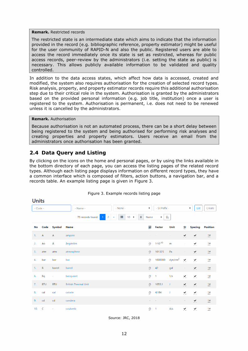
2.4 Data Query and Listing
By clicking on the icons on the home and personal pages, or by using the links available in
the bottom directory of each page, you can access the listing pages of the related record
types. Although each listing page displays information on different record types, they have
a common interface which is composed of filters, action buttons, a navigation bar, and a
records table. An example listing page is given in Figure 3.
Figure 3. Example records listing page
Source: JRC, 2018

13
By default, the listing pages list all records available in the system, which are accessible
by the active user. As indicated before in the data access section, visitors and different
registered users may see different sets of records due to access restrictions. Specific
records can be searched by using the available filters. Multiple filters can be entered at the
same time. The system applies the logical AND operator to combine the filters; hence,
entering multiple filters results in a more restricted query, usually yielding a lower number
of matching records.
In order to perform the query, the "List" button located at the end of the filters should be
clicked. Pressing the "Enter" key on the keyboard while typing on a textual filter also
automatically triggers the query action. Depending on user rights, a "Create" button might
also be displayed next to the "List" button, which leads to the data entry form of the related
record type.
The system features 4 types of filters: textual, drop-down list, date, and existence.
Textual filters allow free-text search by using keywords, which can be further customized
by using special characters and keyword groups. By default, keywords entered in the
textual filters are searched as a whole in the related data fields of the records. For example,
performing a search by entering the keyword degree into the "Name" filter on the "Units"
listing page will return 4 matching records, which are "degree", "degree Celsius", "degree
Fahrenheit", and "degree Rankine". However, the same query with the keyword deg will
return no results, as there are no units in the database which include "deg" as a whole in
the name field.
In order to extend the search to partial words, the asterisk (*) character can be utilized at
the beginning and/or at the end of the keyword. The asterisk is regarded as a placeholder
for zero or more characters, and therefore indicates "starting with", "ending with", or
"including" criteria, if located at the beginning, at the end, or at both sides of a keyword,
respectively. For example, a query with deg* will return the initial 4 matching records, as
all records including the word "degree" also contain a word starting with "deg".
Multiple keywords separated by one or more space characters are combined with the logical
OR operator. Therefore, a query with deg* percent keywords will return 8 records, which
include 4 additional records containing the word "percent": "percent", "percent by volume",
"percent by weight", and "percent standard gravity".
Keyword groups that are composed of multiple keywords can be entered in quotation marks
to prevent evaluation as multiple keywords. For example, the query with deg* cel* will
return 4 degree records matched by the deg* keyword, as the second keyword cel* does
not match additional units. But, the same query with the "deg* cel*" keyword group will
return only one record which is "degree Celsius", as "degree" matches the deg* keyword
and "Celsius" matches the cel* keyword of the keyword group.
Remark. Order of the keywords
The order of the keywords in a keyword group is important and affects how the keywords
are searched. For example, "deg* cel*" and "cel* deg*" are not identical.
In order to exclude a keyword or keyword group, the minus (-) character can be utilized
at the beginning of the keyword or keyword group. For example, deg* -cel* will return 3
records, i.e. all 4 degree records, except "degree Celsius" because "Celsius" matches the
cel* keyword which is excluded.
By entering multiple keywords or keyword groups and utilizing special characters,
advanced queries can be performed easily by using the textual filters.

14
Remark. Textual filters
Textual filters are case insensitive, i.e. lower case and upper case characters are
considered to be identical, unless the related data field of the record is case sensitive.
For example, the degree and DEGREE keywords return the same results. The only
exceptions (i.e. case-sensitive filters) are the filters related to the "Code" data fields of
the "Unit" and "Property" records, as these data fields are case-sensitive.
Drop-down filters match the records which have the same value in the related data field
as the value selected in the drop-down filter. Usually drop-down filters correspond to the
drop-down list input elements of the records and include the options presented by these
input elements. There are also two additional special options available, which are Any and
None. The records having a value (i.e. any value) set or having no value set for the
specified data field can be queried by using the Any and None options, respectively.
Similarly, existence filters check whether or not any value exists in the related data field.
Date filters match the records with the specified date value in the related date field. See
the Date Input section for more details on the date fields.
The records matching the filters, if any, are listed on the listing pages in a tabular format.
Each row in the table corresponds to a separate record. Because some queries may match
a very large number of records, the results are tabulated through pagination, i.e. each
time a limited number of records are tabulated based on the active page number and the
number of rows per page (Figure 3).
Above the results table, a navigation bar is provided which includes tools to navigate
through the results and modify how the results are listed. The first item on the navigation
bar is an indicator, which displays the total number of records in the results set. Next to
the indicator, a pagination element is provided which shows the active page and allows
navigation through the other result pages.
Hint. Rows per page
The default number of rows per page is 25, which can be changed by the "Rows Per
Page" drop-down list next to the pagination element. Setting a new number of rows per
page does not reset the current starting row number. For example, if the current starting
row is 26, then 50 rows starting from the 26th row are displayed if rows per page is
changed from 25 to 50.
Normally, results are tabulated as sorted by the default sorting column of the results table,
which depends on the record type. The sorting column can be changed by using the "Sort
By" drop-down list. The direction of sorting (i.e. ascending or descending) can be specified
by clicking the "Sort Direction" button, which toggles the sorting direction between the
ascending and descending orders. The active sorting column is indicated by a triangle next
to the column name, which points up or down for ascending or descending order,
respectively.
Hint. Local sorting
The sorting settings affect not only the results visible on the active page, but also on all
other pages, i.e. all results matching the query are sorted accordingly. By clicking the
table column labels, you can also sort the results in the current page locally. Similar to
the normal sorting, the sorted column is indicated with a triangle. Successive clicks on
the same label change the sort direction. Local sorting is not permanent, i.e. the sorting
column and direction will reset to the defaults specified in the sorting settings if the active
page is changed or refreshed.

15
2.5 Data Entry
Data entry to the system is done through interactive data forms. You can access the
record-specific data entry forms by clicking the "Create" button displayed on the record
listing pages. Create buttons are also displayed for specific record types on the information
pages of the related records. For example, the industrial plant information page displays a
"Create" button for the "Risk Analysis" record type, which leads to the risk analysis data
entry form and sets the plant data field automatically.
Remark. Display of the "Create" buttons
"Create" buttons are only displayed if the user has the right to create an associated
record. Most of the time being a registered users is enough to create records, but
additional limitations exist for certain record types as indicated in the Data Access
section.
The data entry forms include mobile-friendly and responsive input elements, such as text
fields, drop-down lists, and check boxes, which are common to web-based applications.
There are also some enhanced input elements, such as fuzzy number fields, wiki editors,
calendars, and input lists. The data entry forms also include data entry maps that allow
entry of geographical information, such as coordinates and physical boundaries, the details
of which are given in the Mapping section. The forms are dynamic, i.e. some of the input
elements are shown or hidden according to the values of others. Input elements that must
not be left empty (i.e. which are mandatory) are indicated by an asterisk (*) in their labels.
Textual input elements are generally restricted to the entry of specific types of data, such
as numbers, dates, or coordinates. Usually, such elements are indicated with special icons
appended to the input elements. An example data entry form illustrating different input
elements is shown in Figure 4.
Figure 4. Example data entry form
Source: JRC, 2018
Form data is validated on the client-side before submission of the data to the server for
processing. If empty or invalid input data are found, the related input elements are
highlighted and error messages are displayed to indicate the identified errors (Figure 5).
Form submission is not possible until all invalid inputs are corrected. After the submission,
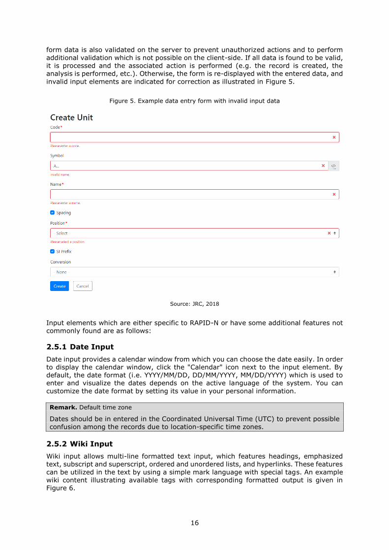
16
form data is also validated on the server to prevent unauthorized actions and to perform
additional validation which is not possible on the client-side. If all data is found to be valid,
it is processed and the associated action is performed (e.g. the record is created, the
analysis is performed, etc.). Otherwise, the form is re-displayed with the entered data, and
invalid input elements are indicated for correction as illustrated in Figure 5.
Figure 5. Example data entry form with invalid input data
Source: JRC, 2018
Input elements which are either specific to RAPID-N or have some additional features not
commonly found are as follows:
2.5.1 Date Input
Date input provides a calendar window from which you can choose the date easily. In order
to display the calendar window, click the "Calendar" icon next to the input element. By
default, the date format (i.e. YYYY/MM/DD, DD/MM/YYYY, MM/DD/YYYY) which is used to
enter and visualize the dates depends on the active language of the system. You can
customize the date format by setting its value in your personal information.
Remark. Default time zone
Dates should be in entered in the Coordinated Universal Time (UTC) to prevent possible
confusion among the records due to location-specific time zones.
2.5.2 Wiki Input
Wiki input allows multi-line formatted text input, which features headings, emphasized
text, subscript and superscript, ordered and unordered lists, and hyperlinks. These features
can be utilized in the text by using a simple mark language with special tags. An example
wiki content illustrating available tags with corresponding formatted output is given in
Figure 6.

17
Figure 6. Example wiki content with corresponding formatted output
== Heading ==
This is a paragraph.
This is another paragraph.
Example '''emphasized''' text.
Example ^^superscript^^ text.
Example ^_subscript_^ text.
Example link: [http://rapidn.jrc.ec.europa.eu]
* Item A
* Item B
* Item C
# First item
# Second item
# Third item
Source: JRC, 2018
2.5.3 Combo Box Input
Combo box input is a combination of a text input and a drop-down list, which allows the
selection of existing values instead of re-typing manually. By clicking the button next to
the input element, text input or drop-down list modes can be toggled.
Remark. Combo boxes
Because they allow standardisation of data values, the use of existing values through the
drop-down list is good practice for combo box inputs.
2.5.4 Fuzzy Number Input
Input data available for the analysis is not always well-defined and can include some
uncertainties. For example, substances often have different values for the same properties
(e.g. heat of combustion) based on the characteristics and limitations of the analysis
methods used to measure the values. Therefore, sometimes data may be available not as
exact numbers, but as range or boundary values such as 2.0 – 2.2, < 10-3, > 0.8, etc. In
order to prevent loss of valuable information by enforcing the users to convert such values
to their point-value approximates for the data entry, the system allows fuzzy numbers to
be entered for numerical data. Signed and unsigned integer, decimal and scientific fuzzy
numbers are supported.
In order to simplify the calculations, five different fuzzy number types are defined in the
system, which describe less than, greater than, in between, about and exact value
conditions that are encountered frequently. Trapezoidal fuzzy numbers with constant
slopes are used to represent fuzzy values (Buckley, 2006). A trapezoidal fuzzy number is
defined by four numbers a ≤ b ≤ c ≤ d, where the base of the trapezoid is the interval
[a, d] and its core is the interval [b, c]. A value of 20% is selected as the default
fuzziness amount, which results in a 20% slope for one-sided conditions (i.e. less than and
greater than) and a 10% slope at sides for the two-sided condition (i.e. about). Examples
of supported fuzzy numbers and their corresponding four-number presentation and
point-value approximations are given in Table 1.

18
Table 1. Supported fuzzy number types
Type Example Definition Point-value
Less than < 8
[6.4, 8.0, 8.0, 8.0] 7.467
Greater than > 8
[8.0, 8.0, 8.8, 9.6] 8.533
Between 7 – 9
[7.0, 7.0, 9.0, 9.0] 8.0
About ~8
[7.2, 8.0, 8.0, 8.8] 8.0
Exact 8
[8.0, 8.0, 8.0, 8.0] 8.0
Source: Girgin, 2012
Remark. Handling of fuzzy numbers
By default, fuzzy numbers are automatically converted to their point-value
approximations for the calculations. The system also has the capability to use fuzzy
arithmetic instead of ordinary arithmetic for the calculations, whenever necessary. In
this case, the results are presented by using the five fuzzy number types supported by
the system, if possible. For example, if the result is [5, 5, 6, 6], it is shown as 5 – 6.
Besides the quantitative uncertainty that can be specified by the fuzzy number types, fuzzy
numbers also support a qualitative uncertainty indicator. By appending a question mark
(?) at the end of the fuzzy number, you can indicate that there is a further uncertainty (i.e.
doubt) on the specified value. For example, 10? indicates that the value might be 10, or
10 - 20? indicates that the value might be between 10 and 20.
Remark. Use of fuzzy numbers
Because fuzzy numbers allow uncertainty in the data to be specified explicitly, they allow
a better representation of the state of the data quality. Therefore, it is good practice to
utilize fuzzy numbers if input data is not well-defined and if it can be represented by the
supported fuzzy number types (i.e. less than, greater than, between, about, and exact).
2.5.5 Unit Input
Most of the numerical data utilized by the system require that the unit of the data to be
specified. For this purpose, the system features unit input elements which allow composite
units to be entered by using a simple format that is composed of base unit codes,
separators, and exponentials. The base units supported by the system and corresponding
unit codes can be accessed through the "Units" listing page, which is available at
http://rapidn.jrc.ec.europa.eu/unit/list.
Codes of the base units that support metric (i.e. SI) prefixes can be combined with
standard SI prefix codes to obtain multiple or fractional units. For example, gram denoted
by g can be prefixed with k to obtain kilogram (kg, 1000 gram), or with m to obtain
milligram (mg, 10-3 gram). A list of SI prefix codes and the corresponding scaling factors is
given in Table 2.
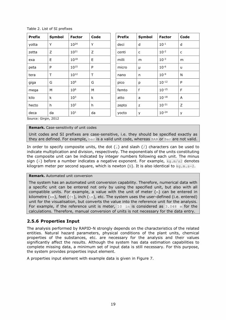
19
Table 2. List of SI prefixes
Prefix Symbol Factor Code Prefix Symbol Factor Code
yotta Y 1024 Y deci d 10-1 d
zetta Z 1021 Z centi c 10-2 c
exa E 1018 E milli m 10-3 m
peta P 1015 P micro μ 10-6 u
tera T 1012 T nano n 10-9 N
giga G 109 G pico p 10-12 P
mega M 106 M femto f 10-15 F
kilo k 103 k atto a 10-18 A
hecto h 102 h zepto z 10-21 Z
deca da 101 da yocto y 10-24 y
Source: Girgin, 2012
Remark. Case-sensitivity of unit codes
Unit codes and SI prefixes are case-sensitive, i.e. they should be specified exactly as
they are defined. For example, bar is a valid unit code, whereas BAR or Bar are not valid.
In order to specify composite units, the dot (.) and slash (/) characters can be used to
indicate multiplication and division, respectively. The exponentials of the units constituting
the composite unit can be indicated by integer numbers following each unit. The minus
sign (-) before a number indicates a negative exponent. For example, kg.m/s2 denotes
kilogram meter per second square, which is newton (N). It is also identical to kg.m.s-2.
Remark. Automated unit conversion
The system has an automated unit conversion capability. Therefore, numerical data with
a specific unit can be entered not only by using the specified unit, but also with all
compatible units. For example, a value with the unit of meter (m) can be entered in
kilometre (km), feet (ft), inch (in), etc. The system uses the user-defined (i.e. entered)
unit for the visualisation, but converts the value into the reference unit for the analysis.
For example, if the reference unit is meter, 10 in is considered as 3.048 m for the
calculations. Therefore, manual conversion of units is not necessary for the data entry.
2.5.6 Properties Input
The analysis performed by RAPID-N strongly depends on the characteristics of the related
entities. Natural hazard parameters, physical conditions of the plant units, chemical
properties of the substances, etc. are necessary for the analysis and their values
significantly affect the results. Although the system has data estimation capabilities to
complete missing data, a minimum set of input data is still necessary. For this purpose,
the system provides properties input element.
A properties input element with example data is given in Figure 7.

20
Figure 7. Example properties input
Source: JRC, 2018
Properties input allows multiple property data to be entered. Each property data includes
the related property and its value together with additional information, such as
measurement unit. Each property can be selected from a drop-down list which lists the
properties that are available (i.e. exists and accessible) in the system that are related to
the record type as grouped by property types.
Hint. Search box
If the number of properties available for a record type is more than 20, the drop-down
list also displays an inline search box which can be used to filter the properties for quick
selection. If a keyword is entered in the search box, only the properties matching the
keyword anywhere in their names, including as part of the words, are displayed. For
example, the vol keyword matches "Volume", "Released Volume", etc.
The input elements presented for the property value depend on the type of the selected
property. For tabular properties, the system uses drop-down list elements from which a
selection can be made. Similar to the property drop-down lists, property value drop-down
lists also feature search boxes if the number of options is high. For numerical properties,
property values can be specified as ordinary or fuzzy numbers in integer, decimal, or
scientific notation. See the Fuzzy Number Input section for details of the fuzzy numbers.
For selected numerical properties the input can be limited to integers only. Similarly,
depending on the nature of the property, possible numerical values might be limited to a
certain range of values (e.g. positive numbers, numbers between 0 – 100, etc.). Numerical
property data inputs may also require the unit of measurement to be specified, which
should be compatible with the reference unit of the related property. The details of the
properties, including the supported data types and validity constraints, are described in
the Properties section.
For each entered property data, the system automatically checks the consistency between
the record type, property, and the property data, including context of the property,
correctness of the data type, correctness of the value, presence and compatibility of the
measurement unit information, and concordance of the entered properties with each other
based on the validity conditions of the properties. For example, the diameter property is
not valid if the shape is set as rectangular or the roof type property is only valid for
cylindrical vertical tanks under atmospheric storage conditions. Problems identified during
the validation are indicated for each property data separately, so that they can be corrected
by the user.
Remark. Data estimation
The system has data estimation capabilities to estimate missing property data by using
other readily available data sources (e.g. maps) or by utilizing its data estimation
framework, which calculates property data by using property-specific estimation
functions. Details of the data estimation capabilities are given in the Data Estimation
Framework section.

21
2.5.7 Conditions Input
Some data utilized by RAPID-N is only valid (i.e. can only be utilized) if certain conditions
are met. For example, the diameter of a plant unit can only be defined if the unit has a
circular cross section. Similarly, a damage function, which can be used to estimate a
damage parameter, can be suitable only for specific natural hazard conditions. In order to
indicate such specific conditions, the system features conditions input elements. A
conditions input element with example condition data is given in Figure 8.
Figure 8. Example conditions input
Source: JRC, 2018
Conditions input allows multiple conditions to be specified. For each condition, the condition
property, condition type, and conditional value (if required) should be specified. Condition
properties can be selected from the properties available in the system that are related to
the record type for which data is entered. The condition type can be selected from a
drop-down list. The system supports three condition types, which are equal to (=), not
equal to (≠), and does not exist (∅). The does not exist condition is valid if the related
property value is not available. It can be used to set validity in case of unavailability of
other property data. Equal to and not equal to condition types test whether the available
property value is the same as the value indicated in the condition (i.e. conditional value).
For tabular condition properties, the conditional value can be selected from the drop-down
list of options provided by the system. For other condition properties, the value should be
entered manually. If the property has a reference unit, the unit of the conditional value
should also be indicated and it has to be compatible with the reference unit.
Remark. Validity of no data
Because they need property data to test the validity, equal to and not equal to conditions
are not valid if property data is not available (i.e. is missing).
Numerical conditions can be entered by using the fuzzy number notation, but in this case
they are regarded as range expressions instead of fuzzy numbers. Example range
expressions and their meanings are illustrated in Table 3.
Table 3. Range expressions for numerical conditions
Expression Description Definition
< 8 Less than 8 𝑥 < 8
> 8 Greater than 8 𝑥 > 8
7 - 9 Between 7 and 9 7 ≤ 𝑥 < 8
8 Exactly 8 𝑥 = 8
Source: Girgin, 2012

22
Multiple conditions can be specified for a single condition property, which are evaluated
with logical OR operators (e.g. Modified Mercalli Intensity, MMI = 5 or = 6 or = 7). Thus,
the validity of a single condition is enough to make the estimator valid for a specific
condition property. Conditions of different condition properties are evaluated with logical
AND operators (e.g. MMI = 5 and Peak Ground Acceleration, PGA ≥ 0.2 g). Therefore, the
validity of all condition properties is necessary to make a conditions list valid.
Conditions are visualized by the system as a comma-separated list of conditions grouped
by condition properties. Example conditions data view is given in Figure 9.
Figure 9. Example condition data view
Source: JRC, 2018
2.6 Mapping
RAPID-N features a mapping system with built-in GIS analysis capabilities for the entry,
visualisation, and analysis of geographical information. The location and boundaries of
natural hazards, industrial plants, and plant units can be easily mapped by using the
interactive map available at the data entry pages. For industrial plants and plant units, a
special mapping tool is also provided, which facilitates entry of multiple records and
delineation of their boundaries. RAPID-N uses Google Maps API for editing geographical
features (i.e. points, polygons, polylines, and circles) and displaying then on the maps.
2.6.1 Editing Features
The basic feature editing functionality provided by the system is identical for the mapping
tool and the maps provided in the data entry pages (i.e. data entry maps). The mapping
tool includes a full screen map which covers the whole page, whereas by default the data
entry maps are limited in size which can be extended, if necessary. A typical map in editing
mode is shown in Figure 10.
Figure 10. Example map in editing mode
Source: JRC, 2018

23
Hint. Full screen map editing
For data entry maps, you can toggle to the full screen map view mode by clicking on the
"Full Screen" button located on the top left corner of the map. While in this mode, clicking
the button again or pressing the "Esc" key on the keyboard will bring you back to the
data entry form with a normal size map.
In order to delineate a feature, first zoom in to the location of the related entity (e.g.
industrial plant) in the map. You can use the zoom in and zoom out buttons located on the
bottom left corner of the map to change the zoom level (Figure 10). Alternatively you can
also use the scroll wheel of your mouse for zooming.
Remark. Use of the "Ctrl" key
For data entry forms, you may need to press the "Ctrl" key on the keyboard while turning
the scroll wheel to enable zooming, otherwise it may scroll the page instead. A "Use ctrl
+ wheel to zoom the map" message is displayed on the map whenever this is necessary.
You can pan the map by clicking a location on the map and dragging it to another location.
By default, the map displays a high-resolution satellite image overlaid with labels, e.g.
street and place names. You can change the map type by using the "Map" and "Satellite"
buttons on the top right corner of the map (Figure 10). In the satellite mode the labels,
and in the map mode the terrain can be toggled on and off by clicking the related
checkboxes, which are displayed when you click on the associated map type button.
Clicking a location on the map initializes the editing process. The system automatically
focuses on the spot and displays a white point and a toolbar on the map (Figure 11.a). You
can easily change the location of the point by dragging and dropping it to somewhere else.
The point can be brought back to the previous location by clicking the "Undo" button that
will be displayed beside the point. The point can be removed completely by clicking the
right-most "Remove" button on the map toolbar and confirming the removal by clicking
"Ok" on the displayed modal dialog. Once the point is deleted, it cannot be undone, but a
new point can be created by clicking the same location on the map.
For point features, the white point indicates the feature itself. For other feature types (i.e.
polygon, polyline, circle) it is only the initial state, which indicates the origin of the feature
without any geometry data. By clicking the "Create Geometry" button on the map toolbar
indicated by a rectangle icon, the point can be converted into a feature with initial geometry
data (i.e. boundary). By default, the system creates a medium sized rectangle, line, or
circle for polygon, polyline, and circle features, respectively.
The initial rectangle boundary for polygon features has 4 "real" vertices on each corner
marked by white points, and 4 "virtual" vertices located at the mid-points of the lines
connecting the real vertices (i.e. boundary lines). The shape of the boundary can be
modified by moving the vertices, i.e. dragging and dropping them to other locations (Figure
11.b). Moving a real vertex deforms the boundary without changing the number of
boundary lines. Therefore, the number of vertices is not affected. On the other hand,
moving a virtual vertex converts it into a real vertex. Subsequently, the original line that
the virtual vertex belongs to is divided into two line segments, for which two additional
virtual vertices are created (Figure 11.c). A real vertex can be removed from the polygon
by right-clicking on the vertex. Once the vertex is removed, two line segments connecting
the vertex to the neighbouring real vertices are also removed and a new line is created to
connect the neighbour vertices to each other (Figure 11.b). By performing successive real
and virtual vertex modifications, the shape of the boundary can be easily modified to match
the physical boundaries of the related entity (e.g. industrial plant) (Figure 11.d). Each
vertex move can be undone by clicking the "Undo" button displayed next to the vertex
after the move. It is also possible to move the whole polygon by dragging and dropping it
to a new location.

24
Figure 11. Polygon editing
(a)
(b)
(c)
(d)
Source: JRC, 2018
Remark. Undo editing
Undo support for vertex moves is limited to a single step, i.e. only the last modification
can be undone. Relocation of a polygon as a whole (i.e. polygon drag-and-drop) cannot
be undone. Similarly, removed vertices can also not be undone. Therefore, you should
create a new vertex at the same location if you want to revert to the previous shape.
For circular features, the map toolbar includes a diameter input tool, which can be used to
set the diameter of the circle manually in meters or feet. Changing the unit, automatically
resizes the circle while keeping its centre fixed. The size (i.e. diameter) of the circle can
also be modified on the map by moving the point markers located on the circle boundary
similar to the vertices of a polygon. Different from the polygons, the number of points is
fixed for circles and limited to 4 for each cardinal direction. One-step undo is available for
each modification. A feature can be removed completely by clicking the "Remove" button
on the map toolbar and confirming the removal. Alternatively, by clicking the "Remove
Geometry" button indicated by a dotted circle on the toolbar, the feature can be converted
into a single point located at the geometric centre of the feature. Clicking the "Zoom"
button on the map toolbar will pan the map to the centre of the feature and set the zoom
level, so that the whole feature is visible on the map with the highest zoom level possible.

25
2.6.2 Data Entry Maps
Data entry maps available at the data entry pages are linked to the input elements of the
associated data entry forms. Whenever you create or modify a feature on the map, the
values of the related input elements are updated automatically.
For example, once you create a point on the map, its coordinates (i.e. latitude and
longitude) will be displayed in the coordinates input of the data entry form and they will
be updated whenever you change the location of the point. Similarly, modifying the
boundaries of a polygon updates the boundaries input. Because changing the boundaries
also usually affects the geometric centre of the feature (i.e. origin), coordinates input will
also be updated automatically.
Hint. Country drop-down list
Besides geometric input elements, the country drop-down list is also linked to the map.
Whenever you choose a country, the map automatically pans and focuses on the
geographic boundaries of the selected country. You can use this feature to facilitate
location finding.
The links to the input elements are operational not only from the map to the inputs, but
also vice versa. So, if you enter or update the coordinates manually in the input field, the
origin of the feature on the map will be updated to reflect the new coordinates.
Hint. Manual input of coordinates
You can use the automated link between the input elements and the map to locate an
entity (e.g. industrial plant), for which coordinate data is available in advance.
Remark. Invalid coordinates
Entering an invalid latitude or longitude in the coordinate input will remove the point on
the map and subsequently clear the manually entered coordinate data, as it is linked to
the map.
By default, the coordinates in the data entry form are displayed in decimal degrees (e.g.
45.5084). But if you want, you can change it into degrees decimal minutes (e.g. 45 30.504)
or degrees minutes seconds (e.g. 45 30 30.24) by changing the coordinate format setting
in your personal page.
Remark. Coordinate format
Coordinate format setting only affects how the coordinates are displayed, but not how
they should be entered. Coordinate inputs can "smartly" detect the format that you use
for data entry and convert them into decimal degrees automatically for storage.
Therefore, you can use any of the three formats to enter coordinates, without performing
a manual conversion. This is especially useful if the coordinate data is originally not
available in the standard decimal degrees format.
Remark. Reference coordinate system
Although the system supports multiple coordinate formats, currently it does not support
user-defined coordinate systems and map projections. The coordinates should be in the
World Geodetic System (WGS 84, EPSG:4326), which is the reference coordinate system
used by the Global Positioning System (GPS).
Although the location of the feature can be modified manually for features with a geometry
(i.e. polygon, polyline, and circle), their boundaries cannot be modified, because the
boundary input is currently read-only.

26
In addition to coordinates and boundary inputs, the circle feature also updates the values
of the "Diameter" and "Radius" properties, if they exist in the properties list of the entity.
If the circle already exists on the map when you add these properties for the first time,
their values are automatically entered by the system and modified subsequently whenever
the circle is modified. Similarly, manually modifying the value of the "Diameter" or "Radius"
property automatically updates the circle on the map, including the diameter input on the
mapping toolbar. Because they are linked, changing the diameter also changes radius, and
vice versa.
Hint. Diameter units
The units of the diameter input tool and the diameter and radius properties are
independent of each other. Hence, they can be set differently (e.g. ft for diameter input
tool, m for diameter or radius property). The system automatically performs unit
conversion and updates the values accordingly.
The system decides the type of feature (i.e. polygon or circle) based on the "Shape"
property. By default, the feature type is set to polygon. Once a "Shape" property is added
to the list of properties and its value is set to one of the following values, the circle editing
mode is activated:
— Cylindrical Dished Vertical
— Cylindrical Hemispheroidal
— Cylindrical Vertical
— Spherical
— Spheroidal
Removing the "Shape" property or changing its value to something different than the
values indicated above, disables circle editing mode and removes the circle on the map, if
it exists. Similarly, activating circle editing mode removes the existing polygon feature.
2.6.3 Mapping Tool
In addition to the data entry maps provided at the data entry pages, RAPID-N also features
a mapping tool specifically designed to map a large number of plants and plant units easily
and quickly. Besides facilitating delineation of the boundaries of plants and plant units, the
tool also allows entry of basic information about the associated records, which can be
further elaborated later through the related data entry forms.
The mapping tool can be accessed by clicking on the "Mapping Tool" icon on the home and
personal pages, or by following the link available in the bottom directory displayed at each
page. For quick access to the tool, you can also use the following URL address:
http://rapidn.jrc.ec.europa.eu/mapping_tool.
The mapping tool provides a map that is similar to the data entry maps, but covers the
whole page area. Zoom in/out buttons located at the bottom right corner, and the map
type selection buttons located at the top left are identical and function as explained in the
Editing Features section. The Full screen button located at the top right corner also exists
and can be used to make the map even larger by covering the full screen.
Different from the data entry maps, the mapping tool also provides a toolbar with several
tool buttons and a search box, which is located at the top left corner of the map. The
toolbar includes the following items (from left to right):
Plant Unit Button activates the plant unit editing mode, which allows you to create new
plant units.
Plant Button activates the industrial plant editing mode, which allows you to create new
plants.

27
Auto-pan Button toggles the automatic map pan mode, which helps you to enter data easily
by panning the map automatically so that the active feature is located at the centre of the
map. By default, it is disabled.
Search Box allows quick zooming to a specific area by entering an address. If you enter a
place name (e.g. city, town, industrial plant, etc.) in the search input and press the "Enter"
key, the system automatically queries and zooms to the boundaries of the specified
location. By using the standard zoom in/out functionality you can focus on the exact
location you are interested in.
Remark. Location search box
If the search query returns information on multiple locations, the first location is
displayed on the map. In order to obtain a single result, you can enter additional
keywords, such as the country or province name, which further restricts the query. If no
results are returned, the existing map location will be kept.
Close Button closes the mapping tool and returns to the personal page.
Once you focus on an area in the mapping tool, either by using the search functionality or
by using the standard zoom in/out – pan features, the system automatically loads the
existing plants and plant units that are located in the map area, which are accessible. Each
plant and plant unit is indicated by a separate map icon (i.e. marker) and the associated
boundaries are also mapped on the map. By clicking on a marker, you can select the related
feature (i.e. plant or plant unit) and open its data window.
Hint. Auto-pan
If auto-pan is enabled, the map will automatically pan to the marker location and the
data window will be opened at the centre of the page.
If you do not have editing access to the selected feature, the data window will only display
information about the related record, such as its name for industrial plants, or type and
shape for the plant units. By clicking on the "Details" link provided at the data window
heading, you can access the information page of the record, from which you can obtain
more detailed information.
If you have editing access to the selected feature, then the editing mode will be activated.
In this case the data window includes input elements, through which you can set or modify
certain properties of the selected record as illustrated in Figure 12. The system also enables
the editing mode for the selected feature, so you can modify the feature (e.g. move, resize,
reshape) as described in detail in the Editing Features section.
The input elements displayed in the data window depend on the type of the selected record.
For industrial plants, only the name input is available. For plant units, you can select the
type (e.g. storage tank, reactor), shape (e.g. cylindrical, spherical), storage condition (e.g.
atmospheric, pressurized), base type (e.g. on-ground, above ground), and roof type (e.g.
fixed roof, floating roof). For both record types it is also possible to enter notes.
The feature type of the plants is a polygon. For plant units, the system automatically selects
the feature type based on the "Shape" property similar to the case of the data entry forms.
See the Data Entry Maps section for the list of shapes that enable circle editing mode.
In order to finish editing and save the changes, you should click on the "Close" button.
Remark. Automated linking of plants and plant units
While saving a plant unit record, the system checks if the associated feature (i.e. polygon
or circle) is located inside a boundary polygon of a plant and if such a plant is found, the
plant unit and the plant are automatically linked to each other (i.e. plant of the plant unit
is set as the identified plant). This facilitates data entry by getting rid of the need to
manually indicate the relation between plant and plant units.

28
Figure 12. Data window in editing mode
Source: JRC, 2018
The editing mode also allows you to delete the record if you are allowed to delete it. In
order to delete the record click on the "Delete" button and confirm it through the modal
dialog which will be displayed.
Remark. Deleting a record
Delete action is irreversible, i.e. can not be undone.
The "Set Default" button indicated by a copy-paste icon located at the bottom of the data
window allows you to set the data of the selected record, including the feature data (i.e.
diameter, boundary), as a template for the new records that will be created.
In order to create a new record, you should first activate either the plant or plant unit
editing mode by clicking the associated buttons on the map toolbar located at the top right
corner. Once an editing mode is activated, clicking on a location on the map will create a
new editable feature and display its associated data window, through which you can set
the record data. If the default data is set previously, the new record will initially contain all
the properties (e.g. name, type, shape, etc.) as defined by the default data and the feature
will also be initialized according to the default feature, i.e. its boundaries or diameter will
be identical to the default feature.
Hint. Quick copy-paste with default data
By setting a record data as the default data, you can easily create clones (i.e. identical
copies) of the record on the map. This is especially useful for large industrial plants (e.g.
refineries), which include many identical plant units (e.g. storage tanks).
You can close the mapping to by clicking on the "Close" button on the map toolbar.
29
3 Data Estimation Framework
RAPID-N features an innovative data estimation framework to minimize the data required
for the data entry and also to calculate the data which is required for the analysis but has
not been or cannot be provided (i.e. entered) by the users.
The framework is based on Properties and Property Estimators, which are described in
detail in the following sections. The steps followed for the data estimation are also
explained in the Data Estimation Methodology section. Besides data estimation purposes,
the framework is also utilized by the system to generate case-specific damage and
consequence models on-demand to perform the calculations necessary for the risk
analysis. Therefore, it forms the backbone of the system.
3.1 Properties
Although they describe different characteristics and attributes, the properties of entities
can be defined in a similar manner. Independent of the entity type (e.g. substance, plant
unit, etc.), each property has a value defined by a number, a string of characters, or a set
of pre-defined options. Generally, units are used to define the scales of numerical values.
Some properties may be conditionally valid. For example, the diameter of a plant unit can
only be defined if it has a spherical or cylindrical shape. Similar conditions also apply for
natural hazard, industrial plant, and substance properties. Considering this similarity,
RAPID-N uses a common framework to define properties of different entities, i.e. records.
Property records are used for this purpose.
Remark. Authorisation
Authorisation is required to create new properties.
An example property data entry form is given in Figure 13. The type of the property
determines the context of the property, i.e. to which record types it is related. It can be
selected from the list of property types available in the system. Each property has a name
and two types of short identifiers: code and symbol. The property code is used to represent
the property in the property estimation functions. The codes should be unique. They are
also case-sensitive. For example, the codes d and D are not identical and refer to different
properties. Symbols, which support subscript, superscript or italic formatting, are used to
represent properties in shorthand notation for display in information pages and record
tables.
Remark. Property codes
In order to facilitate recognition of the properties and to increase the readability of the
estimation functions that utilize the property codes to denote property values, use of
shorthand and abbreviated unit codes should be avoided. It is better practice to use
diameter as the code of the diameter property, instead of only d, as d is not self
explanatory and can be easily confused with properties like density or depth.
The data type defines the nature of the property values. Currently, four different data types
are supported by the system, which are integer, numeric, string and tabular.
The integer data type allows only integer values to be entered, whereas the numeric data
type supports decimal and scientific values, as well. If necessary, fuzzy numbers can be
entered for both numerical data types. They also allow the unit of the property to be
specified. The system treats the unit defined in the property as the reference unit, but also
allows the user to enter values in all possible compatible units. See Unit Input section for
more details on the units.
The string data type allows character strings to be entered as property values. For strings,
Unicode characters are supported which allow a wide range of specialized (e.g.
mathematical) and language specific characters to be entered by the users.

30
Figure 13. Example property data entry form
Source: JRC, 2018
Hint. List of Unicode characters
You can refer to the "List of Unicode characters" page of Wikipedia for a listing of the
Unicode characters by category.
The tabular data type restricts the property value to certain options specified explicitly.
The allowed options must be entered in the options list. For each option, a unique code
and name should be entered. A description of the option can also be specified. An example
tabular property record view is given in Figure 14.
Remark. Option descriptions
Although option descriptions are not utilized for data entry and visualisation, they provide
valuable information about the meaning of the options. Therefore, it is good practice to
provide descriptions, although they are not mandatory.

31
Figure 14. Example tabular property record view
Source: JRC, 2018
For tabular properties, the system uses drop-down list inputs to facilitate data entry. The
options are listed in the drop-down list according to the sorting criteria. If sorting is set as
name or code, the options are listed as sorted by the sorting criteria in ascending order. If
the list order is selected, they are listed according to their order in the options list.
Hint. Search box
For tabular properties including more than 20 options, the system provides an inline
search box, which can be used to filter the options for quick selection. If a keyword is
entered in the search box, only the properties matching the keyword anywhere in their
names, including as part of the words, are displayed
If the property is only valid under certain conditions, validity conditions can be defined by
using the related properties based on property type. For example, the diameter property
can be enabled (i.e. set valid) only for plant units having a circular cross section in any
direction based on the shape property. See Conditions Input section for more information
on the validity conditions and how to enter them.
Additionally, a validation rule can be specified to limit property data entry to certain values.
Validation rules are similar to the single-line functions described in the Estimation Functions
section, in which an x character in square blankets ([x]) denotes the entered value. The
validation rule is evaluated for each entered value of the property, and the value is
considered as valid only if the evaluation result is equal to TRUE. A common use is the
"value greater than zero" rule (i.e. [x] > 0) to allow only unsigned (i.e. positive) values
for numerical properties. See the Estimation Functions section for details on the single-line
functions.

32
Remark. Standard value
For numerical properties, the value of the property in the reference unit is used to
substitute the value parameter in the validation rule (i.e. [x]).
The system features property input elements for entering values of different properties
(i.e. property data) for each record, e.g. natural hazard, industrial plant, plant unit, etc.
See Properties Input section for the details of these input elements.
Available property data is displayed on the information pages of the associated records in
a tabular format that is identical to the basic record data, i.e. data entered by using other
input elements. Each property is indicated by its name, and the corresponding value is
displayed as formatted according to the data type of the property. For numerical properties,
if the unit of a property value is different from the reference unit of the property, its value
in the reference unit is also displayed in parenthesis next to the original value. An example
property data view is given in Figure 15.
Figure 15. Example property data view
Source: JRC, 2018
3.2 Property Estimators
RAPID-N utilizes user-defined property data as input to calculations needed for the
analysis. However, such data may be incomplete in some cases, and in fact it is quite
common to have a lack of information especially on industrial entities (e.g. plants and plant
units). In order to make the analysis possible with minimum data input, the system
features a data estimation framework to calculate missing data by using scientific
estimation methods. The data estimation methodology is generic and independent of the
record type and nature of the property (i.e. the same procedure is used to estimate
property data for different record types).
Property estimators are utilized by the system for three main purposes:
1. To perform calculations necessary for the analysis. The system does not contain any
pre-defined, hard-coded models for the analysis. For each Natech scenario, a flowchart
of the damage and consequence models required for risk analysis is created on demand
by using the property estimators available in the system and all computation is
performed by using the these estimators.
2. To calculate missing property data by using the available property data. For example,
the volume of a plant unit can be calculated geometrically from its dimensions if they
are available. This reduces the amount of data to be entered by the user, as it
eliminates the need to enter data which can be computed by using readily available
information.

33
3. To provide case-specific default values of the properties. For example, a property
estimator can be defined to provide a default value for the topography based on the
location. This usage is similar to making assumptions in calculations and allows the risk
analysis procedure to be completed even with limited data by sacrificing some accuracy.
Use of the property estimators increases the flexibility of the analysis capabilities of
RAPID-N as such estimators can do many calculations that would normally have to be
hard-coded into the system. For example, RAPID-N does not include any built-in functions
for the calculation of plant unit volumes. All volume-related calculations are done by using
property estimators. Therefore, if a new plant unit type with a specific shape is added to
the system, there is no need to update the source code. Only a new property estimator
should be added to support the plant unit, which can be done very easily through the data
entry interface.
Remark. Authorisation
Authorisation is required to create new property estimators.
An example property estimator data entry form is given in Figure 16. For each property
estimator, the property to be estimated should be selected from the list of properties. The
type of the estimator can be selected either as a value or as a function estimator. For value
estimators, the estimated value can be selected from the list of allowed values for tabular
properties or entered as strings or numbers (including fuzzy numbers) for string and
numerical properties, respectively. For function estimators, the estimation function should
be entered which can be a simple single-line function or a complex function involving
conditions, loops, or internal function calls. Estimation functions can utilize values of other
properties, which allows calculation of property values based on other property data. The
value returned by the estimation function should be compatible with the data type of the
estimated property. See the Estimation Functions section for more information on the
estimation functions.
Remark. Use of fuzzy numbers
Although fuzzy numbers are supported both as value estimators and also as the return
values of the function estimators, it is good practice to use exact numbers wherever
possible, since the fuzzy numbers increase the uncertainty of the calculations.
For properties having a reference unit, the unit of the value estimated by the estimator
should be indicated. The specified unit should be compatible with the reference unit of the
property.
If required, the precedence of the property estimator over the other property estimators
of the same property can be specified. The precedence is used while comparing the
estimated values of different estimators during the estimation process. See Data
Estimation Methodology section for more details.
If available, bibliographic references of the property estimator can also be indicated.
Remark. Bibliographic references
In order for a property estimator to be made publicly available, it should be
peer-reviewed for scientific adequacy and validated by comparing some case-study
results with reference data based on measurements or original computations. Both
peer-review and validation tasks require reference documents, which can be consulted
whenever necessary. Therefore it is good practice to provide at least one bibliographic
reference, which provides enough information about the rationale, scope and structure
of the estimation method.

34
Figure 16. Example property estimator data entry form
Source: JRC, 2018
Hint. Entering notes
You can use the notes field of the property estimator to provide additional information
on the estimation method. For example, you can indicate the page number of the
reference that describes the estimation method, or you can provide summary information
about the limitations that cannot be indicated as validity conditions. Because it is a wiki
input element, notes input can include links; therefore, you can refer to other records
available in the system or external resources available on the Internet, if necessary.
The system allows validity conditions to be defined for property estimators to control the
applicability of the estimators, as they may be valid only under certain conditions. For
example, a plant unit volume estimator may be valid only for a certain plant unit shape
(e.g. spherical) or a PGA estimator may be valid for earthquakes having a magnitude
greater than a certain threshold value (e.g. 5.0 in moment magnitude scale). If such
validity conditions exist, a validity test is performed automatically by the system by using
the available data and the estimator is utilized only if the conditions are valid. See
Conditions Input section for more details on the validity conditions.

35
Remark. Validity regions
Previously, property estimators were also featuring validity regions that specified the
geographical extent for which the property estimator was valid. In the current version of
RAPID-N, region records (e.g. countries, Flinn-Engdahl regions, Cratons) are converted
into separate properties with geographic boundaries. Therefore, they can be specified as
validity conditions instead of validity regions.
Example property estimators ranging from default value estimators to complex function
estimators are given in Table 4.
Table 4. Example value and function property estimators
Description Default ambient temperature
Estimator 25 C
Description Wind speed
Estimator 1.5 m/s
Validity Conditions RMP Scenario = Worst-case
Description Storage condition from roof type
Estimator Atmospheric
Validity Conditions Roof Type = Floating Roof, = Internal Floating Roof, = Open Roof
Description Diameter from volume
Estimator pow(6 * [V:m3] / M_PI, 1 / 3)
Validity Conditions Shape = Spherical
Description Energy magnitude from radiated seismic energy
Estimator 2 / 3 * log10([Es:J]) – 2.9
Description Peak Ground Acceleration
Estimator 2000 * exp(0.8 * [M]) * pow([dh:km], -2)
Validity Conditions Flinn-Engdahl Region = [Washington, Oregon, Nevada, …]
Description U.S. EPA RMP Liquid Factor Boiling
Estimator 0.284 * pow([MW:g/mol], 2 / 3) * 760 / (82.05 * [Tb:K])
Description Duration of Fireball
Estimator if ([QFL:kg] > 30000) {
return 0.45 * pow([QFL:kg], 1 / 3);
}
else {
return 2.6 * pow([QFL:kg], 1 / 6);
}
Validity Conditions Fire/Explosion Event = BLEVE
Source: Girgin and Krausmann, 2013a

36
3.3 Data Estimation Methodology
The data estimation framework of the system takes available property data as input and
tries to calculate missing properties by using the available property estimators, taking
validity conditions of the properties and property estimators into consideration. If a value
of a missing property is calculated, it is added to the set of available data and the procedure
is continued recursively until no further properties can be estimated with the available
data, including recently estimated ones.
The steps of the data estimation algorithm are as follows:
1. User-defined property data of the record is retrieved and combined with the basic
record data, which is entered by using input elements other that the properties list
(e.g. name, coordinates, etc.).
2. Associated records of the record, which are explicitly indicated by the reference inputs
(e.g. plant of a plant unit), are retrieved and their record data (i.e. basic record and
property data) are merged with the available data set. The combined data set forms
the data set that is initially available.
3. Property estimators that can be used to estimate properties related to the record are
identified and added to the property estimators list. Property estimators which can
estimate properties that are already available in the data set (i.e. which are user
defined) are excluded.
4. Each property estimator in the property estimators list is examined to determine
whether the available data is enough to evaluate the estimator (i.e. estimator is
eligible):
(a) Because value estimators do not require any other property data, they are
automatically considered as eligible.
(b) For function estimators, the syntax of the estimation function is analysed and the
properties that are utilized in the estimation function are determined. If the
available data include all required properties, the estimator is considered as eligible.
5. For each eligible estimator, conformity with the validity conditions is evaluated by using
the available data. Eligible estimators having valid validity conditions are accepted for
data estimation. See Conditions Input section for more details on the validation
conditions.
6. For each accepted estimator:
(a) If no previous estimate is available for the estimated property, the estimator is used
to estimate the data and the estimated data is added to the available data set.
(b) If a previous estimate is available (i.e. related property data exists in the data set):
i. The priority of the estimators is compared. If the new estimator has a
higher priority than the previous estimator, it is used to estimate data.
The priority check is carried out by applying the following rules in the
listed order:
1. An estimator with a higher precedence is preferred.
2. An estimator with more condition properties is preferred, because
it is assumed to be more specialized (i.e. considers more
properties for validity).
3. An estimator with a lower validity condition score is preferred,
which is calculated by multiplying the number of criteria per
condition property. A lower score indicates that on average there
is a lower number of criteria per condition property, which implies
that the condition is more specialized as the criteria are evaluated
with logical OR operator for each condition property.

37
4. An estimator with a lower dependency score is preferred, which
is calculated by considering the properties utilized by the
estimation function. Estimators that utilize more properties are
considered to be better than the estimators utilizing less
properties, as long as the property data utilized is exact (i.e.
user-defined). If property data estimated in the previous steps is
also utilized, a penalty is added for each estimated property as it
is assumed that there is an accumulation of uncertainty due to
successive estimations.
ii. If the estimator is used to estimate data, the estimated data is compared
with the previous estimate:
1. If the estimates are different (i.e. the new estimate provides a
value different that the previous value), all property data in the
available data set which are related to the previous estimate are
deleted, as they are based on a value which is changed (i.e. not
valid anymore). Property data is considered as related, if it was
estimated by using the previous estimate in the estimation
function or in the validity conditions.
2. Property estimators related to the deleted properties are added
back to the property estimators list.
3. The estimated data is added to the available data set.
(c) If an estimator is used to estimate the data, it is removed from the property
estimators list.
7. If no new property data is estimated or the property estimators list is empty, the
estimation procedure is terminated. Otherwise, the procedure is repeated starting from
Step 3.
Remark. Estimation guarantee
Because it is repetitive, the estimation algorithm is exhaustive, i.e. it guarantees that all
property data is estimated which can be estimated by using the initial data and the
available property estimators.
The estimated property data is highlighted on the record information pages, so that it can
be differentiated from the user-defined properties. An example record data view with
estimated property data is given in Figure 17.
Figure 17. Example record data view with estimated property data
Source: JRC, 2018

38
Remark. Data access in estimation
The available initial data and list of property estimators that can be used for estimation
depend on data access restrictions. Therefore, the final property data available for the
visualisation and the analysis purposes might be different among the users. For example,
private properties are only visible to their owners. Similarly, estimation of a private
estimator is only performed if the active user is the owner of the estimator.

39
4 Risk Analysis Framework
RAPID-N performs Natech risk analysis and mapping in several steps. First, plant units
located in the natural hazard area are identified. Then, the on-site hazard severity
parameters are calculated for each plant unit by using hazard maps, on-site hazard data,
and hazard-specific data estimators. Based on the calculated data, possible structural and
functional damage scenarios are determined and the associated damage probabilities are
calculated by utilizing damage functions and fragility curves. By using risk state definitions,
which relate damage scenarios to consequence scenarios, probable Natech event scenarios
are determined. Finally, the extent and severity of the Natech events are calculated by
using case-specific consequence models generated on-demand and the results are reported
as risk reports and risk maps.
The record types utilized by the system for performing the analysis as summarized above
are described in the following sections. After the presentation of the steps of the risk
analysis methodology, first the records related to natural hazards are explained in detail,
which are followed by the records related to industrial plants, including hazardous
substances. The record types used for damage and consequence analysis are also
described. Finally, the risk analysis records that set-up the risk analysis process are
explained, including important parameters that can be specified to customize the analysis.
4.1 Risk Analysis Methodology
The risk analysis procedure follows the following steps:
1. First, the plants units for which the risk analysis should be performed are identified. If
a plant unit at a plant is specified explicitly, the analysis is limited to the specified plant
unit. If only a plant is specified, the analysis is limited to the plant units located at the
plant. Otherwise, the plant units are selected based on their location with respect to
the extent of the natural hazard event (i.e. hazard boundary). All plant units within the
hazard boundary are included in the analysis. If hazard boundary information is not
available explicitly, the distance to the origin of the hazard is calculated for each plant
unit available in the system and compared to the cut-off distance criteria (i.e. Cut-off
Distance property). Plant units that are within the cut-off distance are selected for the
analysis. If the "Enable Typical Plant Units" property is enabled, "virtual" plant units
are generated for each plant in the proximity of the natural hazard event (i.e. inside
the hazard boundary or cut-off distance) by using the typical plant unit definitions, and
these virtual plant units are included in the analysis.
2. For each identified actual or virtual plant unit, on-site hazard parameters are calculated
in the order listed below. If a parameter value is obtained by using a method, values
obtained by the other methods are discarded (i.e. only the value of the preferred
method is considered).
(a) If manually entered on-site hazard data is available for the risk analysis record,
they are included in the data set.
(b) If on-site hazard data records are available for the specified natural hazard event
which are valid for the plant unit (i.e. belong to the plant where the plant unit is
located), they are included in the data set.
(c) If a custom or default hazard map is specified, the hazard parameters found in the
hazard map are extracted (i.e. interpolated) for the plant unit location and included
in the data set. For virtual plant units, the location of the plant is utilized for the
interpolation.
(d) Hazard-specific property estimators available in the data estimation framework are
utilized to estimate additional parameters by using the available data set.
3. For each identified plant unit, possible damage scenarios are assessed by using
calculated on site hazard parameters and utilizing damage functions (i.e.
damage-related property estimators) and fragility curves available in the system. For

40
this purpose, the validity conditions of the damage functions and fragility curves are
tested by using the available data, and the valid ones are used to determine the extent
and the probability of structural and functional damage states, each of which forms a
specified damage scenario.
4. If the damage probability of a damage scenario cannot be calculated, the state of the
scenario is set as "No Damage Estimate" and it is excluded from the analysis.
5. The calculated damage probability of each damage scenario is compared with the
damage threshold probabilities. The state of the scenarios with a probability less than
the value indicated by the "No Damage Probability" property is set as "No Damage"
and is excluded from the analysis. The state of the scenarios with a probability less
than the value indicated by the "Minimum Damage Probability" is set as "No Damage
Expected" and is excluded from the consequence analysis.
6. If the substance present in a plant unit is not specified, the damage probabilities of the
plant unit are reported and the unit is excluded from the consequence analysis.
7. Available risk states are identified for each damage scenario having an occurrence
probability greater than the minimum threshold probability. For this purpose, risk states
available in the system are examined and their validity conditions are evaluated by
using plant unit, substance, and damage scenario properties. Risk and consequence
scenario parameters specified in the risk states, for which validity conditions are
fulfilled, are merged with the Natech scenario parameters. If the same parameter is
found in multiple risk states, the value of the risk state having the highest precedence
is utilized.
8. The final set of Natech scenario parameters, together with the scenario parameters
indicated in the risk analysis record, are utilized to analyse the consequences. As a
proof-of-concept, the data estimation framework of RAPID-N includes an
implementation of the U.S. EPA RMP Guidance for Offsite Consequence Analysis
(RMP*Comp) methodology (U.S. EPA, 1999) for consequence analysis. All equations
and rules required for the analysis according to the methodology are available in
RAPID-N as property estimators. Suitable combinations of equations are selected by
the system automatically to construct the case-specific flowchart of the methodology
for each Natech scenario, including enhancements provided by the additional methods
and equations (i.e. property estimators) available in the system.
9. The results of the risk analysis are presented as summary reports and interactive risk
maps showing Natech event probabilities and the areas possibly affected by the events.
Use of the data estimation framework for the analysis allows parameters used by the
equations to be modified and alternative equations to be substituted easily. For example,
fire-related end-point distance criteria, which are set as second-degree burns, can be easily
changed to first or third degree burns, or the atmospheric dispersion model, which uses
lookup tables, can be substituted with a more advanced model if necessary. By modifying
the damage parameters, different scenarios can be evaluated without any modifications to
the system code and without any disturbance to the existing system functionality. Also
customized versions of the models for different users are possible.
4.2 References
Many records in RAPID-N, which are utilized for risk analysis, are based on the information
available in the scientific and technical literature. Specifying the original information
sources is not only important for proper citation of the work, but also for quality control
and assurance. It also allows users to access more detailed information when necessary.
The system provides a bibliographic database, which allows detailed bibliographic
information to be stored and linked to the related records. Reference records are used to
store bibliographic information.

41
An example reference record is given in Figure 18. A wide variety of bibliographic
references, such as journal articles, books, and technical reports are supported. Data fields
of reference records depend on the reference type, i.e. different data field combinations
are requested for each reference type. Reference types and their required and optional
data fields are based on BibTex entry types, which is a widely used reference management
system (Patashnik, 1988).
Figure 18. Example reference record view
Source: JRC, 2018
Remark. Author and editor names
The names of the authors and editors should be entered as separated by semi-colon (;).
Do not use and as a separator, as it is not recognized by the system as a separator.
Hint. Full names
It is a good practice to provide full names instead of initials, whenever possible. The
system automatically formats the names to shorten the list of authors and editors by
using initials and "et al." postfix if necessary.

42
Hint. Combo boxes
Journal, institution, publisher, and school fields are provided as combo boxes listing
previously entered values for selection and also allowing to enter new values, if
necessary. Selecting an existing value not only facilitates data entry, but also helps
standardisation of the values.
The system allows electronic copies of the references to be stored as files attached to the
reference records. Multiple files can be uploaded for each reference. The source URL can
be indicated and access rights can be set for each file separately. Public files are available
to everyone for viewing or downloading, whereas private files can only be accessed by the
user who uploaded the file (i.e. owner).
Remark. Document upload
Copyrighted documents should not be made publicly accessible. For documents that are
already publicly available on the Internet, it is good practice to provide the URL address
and also upload a copy of the document to the system. This ensures that the document
is accessible to the users even if the original source becomes unavailable or inaccessible,
which is quite common for URLs that are not permanent.
4.3 Hazards
Information on historical or scenario natural hazard events which can be used for Natech
risk analysis purposes are stored in the hazard records.
An example hazard data entry form is given in Figure 19. For each hazard, the hazard type,
a descriptive name, and the occurrence date should be specified. The location of the hazard
can be stated by country and province. The country list is linked to the map and updates
the map extent to display the selected country. The origin of the hazard can be indicated
either by entering the coordinates manually or by marking them on the map. Similarly, the
hazard area can be mapped as the hazard boundary. See the Mapping section for more
details on the mapping support of the system and how to edit map features.
RAPID-N allows hazard maps to be defined for each hazard entity, which provide
site-specific hazard severity data. One of the hazard maps associated to the hazard event
can be selected as the default hazard map. The default hazard map is utilized to calculate
on-site hazard parameters whenever necessary, unless a custom hazard map is selected
by the user. Details on the hazard maps are given in the Hazard Maps section.
Detailed information on hazard properties at the source (e.g. magnitude, intensity) can be
specified by entering property values to the properties list. Depending on the selected
hazard type, the system only lists properties that are valid for the hazard type.
By using the property estimators, additional hazard parameters are calculated by the
system and are displayed on the hazard information page. Other records related to the
hazard can also be accessed from the information page, including catalogue data of the
event, hazard maps which contain regional on-site hazard parameters for the event,
Natechs that were triggered by the event, and risk analyses already performed by using
the hazard event as the trigger. An example hazard information page is given in Figure 20.
RAPID-N has data extraction and importing capabilities which are used to keep track of
recent natural hazard events (e.g. earthquakes) and to obtain and harmonize data
automatically that can be used for Natech risk analysis purposes. The system monitors
online data feeds of the U.S. Geological Survey (USGS) and European-Mediterranean
Seismological Centre (EMSC) in near real-time for earthquakes having a magnitude greater
than M 5.5. Currently, the natural hazard database of RAPID-N contains information about
21,000 earthquakes, which is publicly available.

43
Figure 19. Example hazard data entry form
Source: JRC, 2018

44
Figure 20. Example hazard information page
Source: JRC, 2018

45
RAPID-N is also capable of estimating site-specific (i.e. on-site) hazard parameters (e.g.
intensity, peak ground acceleration) based on the source parameters (e.g. location,
magnitude, focal depth). For this purpose, hazard-specific property estimators available in
the system are used. However, the system can also utilize pre-calculated or measured (for
historical events) on-site hazard data if readily available. Such data can be entered in two
ways:
— Regional hazard data can be uploaded to the system as hazard maps, which include
multi variate hazard parameters.
— Site-specific hazard data can be entered manually as on-site hazard data records.
4.4 Hazard Maps
Hazard maps in various formats can be uploaded to the system as hazard map records.
Each hazard map is linked to a single hazard, but each hazard may have multiple hazard
maps which might have different extents, scales (i.e. resolutions), and accuracies. Hazard
maps may be multi-variate, i.e. contain multiple on-site hazard parameter data in a single
map.
Hint. Use of hazard maps
Hazard maps produced by systems or software packages specifically designed for this
purpose usually provide better and more accurate data compared to the estimators
available in RAPID-N. Therefore, whenever possible, use of hazard maps is recommended
for the analysis.
Currently, three types of hazard maps are supported by the system: ShakeMap XML,
Gzipped ShakeMap XML and ShakeMap Grid. All these types are used for earthquakes and
include tabular peak ground acceleration (PGA), peak ground velocity (PGV), modified
Mercalli intensity (MMI), and spectral acceleration (SA) data in a regular latitude and
longitude grid. Details of the formats can be found in the ShakeMap Manual (Wald et al.,
2005).
Remark. Large hazard maps
For processing a gridded hazard map which covers a large area in fine resolution (i.e.
small grid size) the system needs a significant amount of memory. If you encounter
problems during the analysis while using such a maps, please substitute the map with a
smaller extent or coarser resolution map.
An example hazard map data entry form is given in Figure 21. For each hazard map, the
associated natural hazard event should be selected from the list of hazards available in the
system. The type of the hazard map should be specified, which has to be inline with the
uploaded map file. Production date and source URL of the hazard map can be indicated
and descriptive notes can be entered. At least one bibliographical reference should be
provided for each hazard map.
Remark. Hazard map boundaries
The boundaries of the hazard map are automatically calculated by the system. Available
industrial plants within the map boundaries are also automatically determined and
displayed on the hazard map information page.
Hint. Non-gridded hazard Maps
The system only supports maps in gridded format and calculates on-site values by using
2-D spatial interpolation. If you have hazard maps in other formats (e.g. vector, raster),
you can use a GIS software to convert your files into one of the supported grid formats.
Open-source GIS software (e.g. QGIS, GRASS GIS) can be used for this purpose.

46
Figure 21. Example hazard map data entry form
Source: JRC, 2018
RAPID-N periodically monitors the ShakeMaps archive of the USGS, downloads recently
published ShakeMaps, and automatically creates the associated hazard map records in the
system, which can be used for Natech risk analysis purposes. Currently, RAPID-N contains
about 11,600 ShakeMaps, which can be used for Natech risk analysis purposes.
4.5 Industrial Plants
Information on industrial plants are stored in the system as plant records. Data on plants
includes the name and the operator of the plant, descriptive and geographic location
information, and the plant properties such as operational, environmental and
meteorological conditions.
An example plant data entry form is given in Figure 22. For each plant, a plant name should
be specified. The operator of the plant can be selected from the operator records entered
into the system, which include the name of the operator, country of origin, and contact
information including postal address, phone numbers, and web site. Descriptive location
information of a plant includes country, province, city and address. The geographic location
of the plant can be indicated as coordinates or mapped on the map as plant boundaries.
See the Mapping section for more details on mapping plant coordinates and boundaries.

47
Delineation of the plant boundaries is useful for several purposes. Besides indicating the
geographical extent of the plant, it also helps identification of on-site and off-site
consequences of potential Natech accidents. Based on the boundary data, RAPID-N can
also calculate some additional parameters, such as surface area, proximity to other plants,
etc., which can be useful for the analysis. Finally, if boundary data exists, the system can
automatically link plant units that are created through the plant unit data entry form or
the mapping tool to the plant that they are physically located in. Hence, it facilitates data
entry by getting rid of the need to manually indicate the relation between plant and plant
units.
The characteristics of the plant can be indicated by adding property values to the properties
list. Plant properties are divided into two groups: The first group is related to the physical
and operational properties of the plant, such as industrial activity, year of construction,
and number of employees. The second group is related to the plant site and its
surroundings. Environmental (e.g. topography, soil class) and meteorological (e.g. ambient
temperature) conditions can be given as examples of the properties in this group.
Remark. Activity and status of an industrial plant
You can indicate the type of industrial activity by using the "NACE Code" property.
Similarly, the operational status of the plant (e.g. operational, shutdown) can be
indicated by using the "Operational Status" property.
Hint. Site-related properties
Site-related plant properties are considered to be valid also for the plant units located at
the plant, if plant-unit specific values are not provided. Because many site-related
properties are not expected to change within a plant, it is good practice to enter such
properties into plant records and to enter customized properties to the plant units only
if it is necessary. Besides reducing data entry efforts, this practice also facilitates data
updates as updating only the plant record will automatically affect all linked plant units.
The records related to the plant can be accessed from the plant information page, which
include plant units of the plant, the on-site hazard specified for the plant for different
natural hazard events, Natechs that occurred at the plant, and risk analyses that include
the plant. An example plant information page is given in Figure 23.
The system includes data for more than 5,500 industrial plants world-wide, which is
collected from public sources, such as the Global Energy Observatory. Basic information
on all petroleum refineries and most of the power plants are available. However, due to
confidentiality reasons this data is not publicly accessible. In order to access the data,
please contact the administrators by using the Contact Form of RAPID-N.

48
Figure 22. Example plant data entry form
Source: JRC, 2018

49
Figure 23. Example plant information page
Source: JRC, 2018

50
4.6 Plant Units
The Natech risk analysis methodology of RAPID-N is based on the estimation of Natech
scenarios for plant units located at industrial plants. Hence, the focus is on plant units and
their characteristics, including their structural and functional behaviour against natural
hazard impacts and the hazardous substances present therein.
Although there are different types of plant units in an industrial plant, Natech risk analysis
methodologies developed so far mainly focused on storage tanks. Since Natech events are
directly related with hazardous substances, and storage tanks generally contain such
substances in large quantities, it is reasonable to give priority to storage tanks. However,
other types of plant units are also important and may cause major Natech accidents. For
this purpose, RAPID-N supports not only storage tanks, but also other types of plant units.
An example plant unit data entry form is given in Figure 24. For each plant unit, the type
of unit (e.g. storage tank, reactor), the industrial plant that the unit belongs to, a unique
plant unit code, descriptive and geographic location, and the substance contained within
the unit can be indicated. Additional data, such as dimensions, structural characteristics,
and safety measures, can be entered as property values in the properties list.
The system allows a plant unit to be present without being linked to a specific plant. This
is mainly to support plant unit data originating from 3rd party sources, such as open
collaborative mapping projects, which can provide geographic data on plant units (e.g.
storage tanks) without explicit reference to associated plants. Therefore, only the unit type
is mandatory as input. However, entry of other data including some properties is necessary
for carrying out a risk analysis.
Remark. Associated plants
RAPID-N automatically transfers site-specific properties (e.g. on-site hazard parameters,
meteorological conditions), from the related plant record to the plant unit record, if
plant-unit specific values are not specified. Therefore, indicating the plant of the unit is
useful for the analysis.
You can indicate the location of the plant unit and delineate its boundaries on the map as
described in detail in the Mapping section. The delineation process is identical, but
enhanced for plant units with circular cross section (e.g. cylindrical storage tanks). Because
the boundaries of such plant units are better described by circles instead of polygons, the
system automatically switches to circle editing mode based on the "Shape" property.
Because the feature editing mode depends on the "Shape" property, but not the type of
the plant unit, circular editing is not limited to storage tanks. You can also delineate other
circular units, such as columns or stacks.
Hint. Plant unit location
The location of the unit is used to map the extent of the estimated consequences as part
of the Natech risk analysis. Hence, it is necessary to provide the location data to obtain
proper Natech risk maps at the end of the analysis.
The substance stored in the plant unit can be specified by selecting a substance from the
list of substances available in the system. If the substance stored in the plant unit is not
specified, the system cannot determine the potential consequences during the Natech risk
analysis. Therefore, in the absence of the substance information, consequence analysis
cannot be performed and only the results of the damage analysis can be reported.
Hint. Substance data
For a complete risk analysis, the substance stored in the plant unit must be specified. If
the substance cannot be identified with certainty, a substance that has similar hazardous
characteristics to the actual substance can be specified as a substitute. For example,
Kerosene can be used as a substitute for fuels which are not very volatile.

51
Figure 24. Example plant unit data entry form
Source: JRC, 2018

52
The availability of data on other plant characteristics is also important and directly affects
the analysis process. Although the system tries to estimate the missing data, the more
data is provided to the estimation framework as input, the better and accurate the
estimates will be. Therefore, it is good practice to provide all available data for each plant
unit to the system.
Remark. Plant unit type
The list of plant unit properties that can be entered for each unit depends on the type of
the unit. Therefore, before entering the properties make sure that you choose the proper
plant unit type.
The extent and severity of the Natech-related consequences mainly depend on the hazard
characteristics and amount of the hazardous substance stored in the plant unit. Therefore,
plant unit properties that allow the calculation of this information are important for the
analysis. Besides the substance, at minimum the following properties should be provided
for a proper analysis:
— Volume (either directly or by providing unit dimensions, e.g. diameter and height)
— Filling level (either directly or by providing filling percentage or filled volume)
— Storage condition (either as category, e.g. atmospheric or pressurised, or by providing
storage pressure and temperature)
Providing the following properties is also highly recommended to increase the accuracy of
the analysis:
— Shape
— Dimensions (e.g. height, length, diameter)
— Base type (e.g. on-ground, above ground)
— Base support (e.g. anchorage)
— Mitigation measures (e.g. secondary containment or dike, if possible with dimensions)
Although the data in the form given in Figure 24 is not complete, it illustrates the minimum
information which should be provided. As indicated before, the system is capable of
estimating additional property data by using the available data. Figure 25, which is the
information page corresponding to the plant unit data entered in Figure 24, illustrates this
capability. In the figure, the properties indicated in red are estimated by the system.
The system includes data on more than 64,000 plant units, mainly storage tanks,
world-wide, which is collected from public sources, such as OpenStreetMap. However, due
to confidentiality reasons this data is not publicly accessible. In order to access the data,
please contact the administrators by using the Contact Form of RAPID-N.
4.7 Typical Plant Units
As indicated before, RAPID-N requires plant unit data for the estimation of Natech risk,
which can be entered as plant unit records. However, plant unit data may not be available
for each industrial plant. Especially for regional studies, it is quite common to have only
summary plant information with some indicators such as industrial activity, production
capacity, and total amount of hazardous substances present, but without specific details
of the plant units. For such plants, RAPID-N can assume which kind of plant units might be
present based on standard plant configurations and can perform the risk analysis
accordingly. Typical plant unit records are used to provide information on such
representative plant units, including characteristic properties, related hazardous
substance, and validity conditions.

53
Figure 25. Example plant unit data information page
Source: JRC, 2018

54
Similar to plant units, for each typical plant unit the type of the plant unit should be
specified. A descriptive code number (e.g. TPU-001) can be indicated. The substance stored
in the typical plant unit can be specified by selecting a substance from the list of substances
available in the system. The characteristics of the typical plant unit, including dimensions,
storage conditions, and amount of the substance stored, can be indicated by entering
property values in the properties list. Similar to the plant units, the system only lists
properties valid for the selected plant unit type. See Properties Input section for more
details on property data entry.
Different from the plant units, validity conditions can be specified for each typical plant
unit to indicate their applicability. All plant properties are available as condition properties.
Hence, a typical plant unit can be defined, for example, for plants with specific type of
activity, location, production capacity, construction date, or combinations thereof. See the
Conditions Input section for more details on the validity conditions.
Hint. Benefits of typical plant units
Typical plant units can be very useful to obtain a preliminary Natech risk analysis without
having to collect detailed information on the actual plant units. By creating various typical
plant units representative of different industrial activities and carefully setting their
validity conditions, regional preliminary risk analysis studies can be performed easily and
quickly. For example, you can specify "NACE Code" properties as validity conditions to
limit typical plant units to specific industrial activities.
Remark. Location of typical plant units
Although the typical plant units are processed like the actual plant units and yield similar
analysis results, they don't have physical coordinates because they are "virtual".
Therefore, they are listed in the risk reports, but cannot be shown on the risk maps.
Because they do not have location information, in order to estimate location-related
properties (e.g. distance to the hazard origin) the coordinates of the plant are utilized
for all typical units of the plant.
4.8 Substances
The consequences of Natech events mainly depend on the quantity, storage conditions,
and hazardous characteristics of the substances involved in the event. For example, fire is
probable only if the released substance is flammable. For volatile liquids, the amount that
will be dispersed into the atmosphere is a function of boiling point and vapour pressure.
The threshold concentrations of toxic substances also differ from substance to substance.
In order to provide such substance data required for the analysis, RAPID-N features a
substance database that includes information on the physical, chemical, and hazardous
properties of the substances.
An example substance data entry form is given in Figure 26. The information on substances
includes name, identifier and structure data. Substance names may contain symbols and
special formatting, such as italic, subscript and superscript. Multiple names of a substance
can be entered by using semi-colon (;) as separator. Frequently used chemical identifiers
can also be indicated to facilitate access to substances. Supported identifiers are:
— CAS No: Chemical Abstracts Service (CAS) Registry number of the American Chemical
Society,
— EC No: European Inventory of Existing Chemical Substances (EINECS), and European
List of Notified Chemical Substances (ELINCS) number of the European Union,
— EC Index No: 67/548/EEC Directive Annex I index number.

55
Figure 26. Example substance data entry form
Source: JRC, 2018

56
Information on the structure of the substance is stored as textual chemical formula and
formatted strings in International Chemical Identifier (InChI) (Stein et al., 2003) and
Simplified Molecular Input Line Entry Specification (SMILES) (Weininger, 1988) notations.
Besides giving insight into the chemical structure of the substance, these identifiers can
also be used to estimate chemical properties by using structure-property relationships.
The properties of a substance can be indicated by using the properties list. There are three
types of substance properties which are used for the analysis. The first one is
physicochemical properties, such as molecular weight and boiling point. The second one is
hazard properties, which includes toxic concentration thresholds and other hazardous
characteristics (e.g. flammability limits). The last category is specific to the consequence
calculations by using U.S. EPA's RMP Guidance for Offsite Consequence Analysis
(RMP*Comp) methodology (U.S. EPA, 1999) and includes properties related to substance-
specific factors, which are utilized to facilitate computations. See Properties Input section
for more details on property data entry.
Remark. Temperature-dependent properties
For temperature-dependent properties, such as density or viscosity, the value at a
reference temperature (25ºC) should be provided. The system utilises correction factors
to calculate the corresponding values in different temperatures according to the
RMP*Comp methodology. See U.S. EPA (1999) for more details.
The minimum data required for calculating the extent of consequences (i.e. heat radiation,
overpressure, toxic concentration) depends on the type of consequence and models used
for the computation. However, as a rule of thumb, the following properties should be
provided for a substance to make the consequence analysis possible:
For all substances:
— Molecular Weight
— Density
— Vapour Pressure
— Boiling Point
— Heat of Vaporisation
For toxic substances:
— Toxic Threshold Concentration
For flammable substances:
— Heat of Combustion
— Heat Capacity
— Specific Heat Ratio
— Lower Flammability Limit
— Upper Flammability Limit
4.9 Damage Classifications
The estimation of the potential damage to a plant unit due to a natural hazard event is
based on the calculation of the probabilities of certain damage scenarios given a set of
on-site natural hazard parameters. Because the extent of damage is highly case-specific
and varies significantly, a simplification is usually necessary to facilitate the analysis.
Generally, this is done by grouping similar damage scenarios into a set of damage states,
ranging from no damage to complete damage gradually in several steps (U.S. FEMA, 1997).
Damage states also form the basis of fragility curves, which are frequently used for damage
assessment. Therefore, they are supported by RAPID-N.

57
An example damage classification record is given in Figure 27. Since damage states are
natural hazard specific, a hazard type should be selected for each damage classification
record. The name of the damage classification and a short description should be provided.
By default, the damage classification is valid for all plant unit types. A plant unit type can
be specified explicitly, if the damage classification is only valid for that plant unit type (e.g.
storage tank).
Multiple damage states can be defined for each damage classification. They are identified
by damage classification-specific unique codes. Common practice is to use sequential
numbers prefixed by "DS", e.g. DS1, DS2, etc. If available, short labels such as "None",
"Light", "Moderate" can also be specified. A description of each damage state should be
provided to indicate the type and extent of damage defined by the damage state.
Bibliographic references of the damage classification can be indicated by selecting the
references from the reference records available in the system or by entering a new
reference. At least one reference is mandatory.
Figure 27. Example damage classification
Source: JRC, 2018
Hint. Alternatives to damage classifications
Although they are frequently used, damage states are not the only way to describe the
possible damage. There are also other methods available, which allow better
quantification of the damage. It is good practice to utilize such methods instead of
damage states, as quantitative damage scenarios can be more easily and accurately
linked to the related consequence scenarios.

58
4.10 Fragility Curves
Fragility curves are X-Y plots relating a hazard parameter (e.g. PGA) to the damage
probability of a structure for a certain damage state (U.S. FEMA, 1997). They are frequently
used to estimate natural hazard damage to engineered structures such as housing, bridges,
or plant units. Typically, fragility curves related to plant units are prepared by statistical
analysis of historical event data (e.g. O'Rourke and So, 2000). Fragility curves based on
numerical analysis and modelling studies are also available (e.g. Berahman and
Behnamfar, 2009). RAPID-N supports fragility curves in the damage estimation part of the
risk analysis.
An example fragility curve data entry form is given in Figure 28. For each fragility curve, a
descriptive name and an abbreviation should be provided. The damage classification that
the fragility curve is based on should be selected. The type of plant unit, for which the
fragility curve is valid (e.g. storage tank), should be specified. The hazard parameter (i.e.
independent variable) of the fragility curve should be selected from the list of hazard
parameters (e.g. PGA). If the parameter is a numerical property with a reference unit, the
unit used for the fragility curve should also be indicated.
Curve data should be entered separately for each damage state. The system supports
different functional forms for the curves, each of which require a different set of
parameters. The supported functional forms with required parameters and corresponding
functions are listed in Table 5.
Table 5. Functional forms supported for fragility curves
Functional Form Parameters Equation
Log-normal (median) Median (m)
Standard deviation (σ)
2
lnlnerf1
2
1
mx
Log-normal (mean) Mean (μ)
Standard deviation (σ)
2
lnerf1
2
1
x
Probit k1
k2
2
5)ln((erf1
2
1 21 xkk
Dataset Parameter values
Probabilities Quadratic Interpolation
Source: Girgin, 2012
In addition to different functional forms, the system also supports two different types of
curves which are discrete and cumulative. A discrete curve defines the damage probability
only for the specified damage state. Therefore, it defines an "equal" condition, e.g. = DS2.
On the other hand, a cumulative curve defines the overall damage probability for the
specified damage state and all other damage states above it. Therefore, it defines a
"greater than or equal" condition, e.g. ≥ DS2. The proper curve type should be selected
depending on the available curve data.
Remark. Discrete and cumulative curves
The system utilizes discrete curves for the analysis. But it also has the capability to
transform cumulative curves into discrete curves, and vice versa. Therefore, the curve
type does not affect the analysis.

59
Figure 28. Example fragility curve data entry form
Source: JRC, 2018

60
Remark. Damage states
Curve data is not mandatory for all damages states. Therefore, a subset of the damage
states can be used for data entry. However, it is good practice to provide data for all
damage states, so that the probability of each damage state can be explicitly calculated.
Otherwise, the system cannot successfully develop Natech scenarios, and also curve
transformation cannot be performed.
Similar to the property estimators, validity conditions can be specified for fragility curves.
Therefore, a fragility curve can be restricted to a specific plant unit type with certain
characteristics (e.g. atmospheric fixed-roof cylindrical storage tanks). See Conditions Input
section for more details on the validity conditions.
For each fragility curve, bibliographic references should be indicated to provide information
on the origin of the curve data. At least one reference is mandatory.
Fragility curve information is presented in tabular form together with curve data, validity
conditions, and bibliographic references. Interactive fragility curve plots are provided for
each damage state. The curves are plotted on the same graph, so that they can be
compared easily. By moving the mouse pointer over the curves, numerical values of
damage probabilities can be obtained. Based on the available data, both cumulative and
discrete curves are calculated automatically and displayed separately. Example fragility
curves, which are based on the data given in Figure 28, are shown in Figure 29.
Figure 29. Example cumulative and discrete fragility curves
Source: JRC, 2018

61
Hint. Alternatives to fragility curves
Use of fragility curves is not the only way to provide damage data. Damage-related
property estimators can also be used for the same purpose.
4.11 Risk States
In order to estimate the risk of Natech events, damage scenarios which are calculated by
using on site hazard parameters and damage functions, have to be related to appropriate
consequence scenarios. Similar to the simplification applied in describing damage scenarios
by using damage states, possible consequence scenarios are also simplified as risk states
to facilitate the analysis.
In the past, simple one-to-one relations were used in the literature to relate damage states
to risk states (Salzano et al., 2003; Fabbrocino et al., 2005). Going one step further,
RAPID-N supports conditional risk state definitions for each damage scenario. Conditional
risk states allow different consequence scenarios to be defined for a single damage
scenario, depending on plant unit properties (e.g. storage condition, construction material,
volume), substance properties (e.g. type of substance, boiling point, vapour pressure),
and damage properties (e.g. damage state).
For each risk state, a damage classification and related damage state should be specified.
Scenario parameters, which should be taken into consideration during consequence
analysis, can be specified. These parameters may include source-term parameters (e.g.
release rate, release duration, hole dimensions, pool area, evaporation rate), analysis
parameters (e.g. type of accident scenario, conditional release probability), and
consequence parameters (e.g. fire/explosion event, threshold concentration). See
Properties Input section for more details on property data entry.
The possibility to indicate custom scenario parameters allows damage-scenario specific
non-linear damage-consequence relations to be defined in RAPID-N. This results in a more
realistic risk analysis, for example in the case of damage to piping with significant loss of
content which is generally regarded as minor structural damage, or elephant-foot buckling
with minor loss of content which is generally regarded as major structural damage. In such
cases, classical damage-consequence relations would result in the over- or
under-estimation of the Natech risk due to their linear behaviour, where a higher damage
implies a higher consequence.
Similar to the case of property estimators, validity conditions of a risk state can be indicated
by selecting the appropriate condition properties and setting the criteria. Because
consequence scenarios strongly depend on plant unit conditions and substance
characteristics, both plant unit and substance related properties can be specified as
conditional properties. For example, risk states can be defined for atmospheric floating roof
tanks constructed before a certain date, in which substances with a high heat of combustion
are stored. See Conditions Input section for more details on the validity conditions.
Remark. Multiple risk states
For a specific damage scenario, all risk states that fulfil the validity conditions are merged
by the system while developing the final consequence scenario. Therefore, more complex
scenarios can be obtained by the combination of simpler risk states.
Hint. Use of multiple risk states
Combination of various risk states allows very detailed and case-specific Natech
scenarios to be defined, without disabling generic risk state definitions applicable to other
common situations. It is good practice to define less complex, but multiple risk states,
which can be combined by the system whenever necessary.

62
4.12 Risk Analyses
Natech risk analysis is highly automatized in RAPID-N. The risk analysis data entry form is
rather simple and involves only a couple of input elements. But customisation of the various
stages of the analysis, including hazard analysis, damage analysis, and consequence
analysis, is also possible through several mechanisms and also by setting the values of
related risk analysis properties.
Remark. Authorisation
Authorisation is required to create new risk analyses.
An example risk analysis data entry form is given in Figure 30. For each risk analysis, only
the name of the analysis and the triggering natural hazard event are necessary. The natural
hazard event can be selected from the hazard records available in the system. See the
Hazards section for detailed information on natural hazard records, including how to define
custom hazard events. Once the hazard record is selected, the system automatically lists
available hazards maps related to the hazard record. Selecting a map from the list enforces
the system to use the indicated hazard map to calculate on-site hazard parameters. If the
"Default" option is selected, the default hazard map indicated in the hazard record is
utilized.
Figure 30. Example risk analysis data entry form
Source: JRC, 2018

63
Remark. Use of hazard maps
The specified hazard map is only used to calculate the on-site hazard parameters
available in the hazard map (e.g. PGA, PGV, MMI, and SA for a ShakeMap). Other on-site
hazard parameters, which can be estimated by using available data, including data
originating from the hazard map, are estimated by the data estimation framework and
included in the analysis. Therefore, use of a hazard map does not limit the calculated
on-site hazard parameters to certain parameters. Instead, it supports further estimation
of other parameters by providing accurate input data.
Hint. Default hazard map
For the hazard records publicly available in the system, the default hazard map is
updated automatically by the system whenever a new hazard map becomes available.
Therefore, a default hazard map is usually the best available hazard map for a hazard
record. Hence, the use of default maps is suggested for the analysis.
If the analysis should be restricted to a specific industrial plant (i.e. plant units located at
the plant), the plant can be selected from the plant records available in the system. See
Industrial Plants section for detailed information on plant records. If necessary, the analysis
can be further restricted to a specific plant unit located at the plant by selecting the plant
unit from the list of plant units. By default, all plant units of the plant are included in the
analysis.
If a plant is selected, the system allows site-specific hazard parameters to be entered
manually in the risk analysis data entry form. Therefore, in addition to the hazard maps
and on-site hazard data, risk-analysis specific on-site hazard data can also be specified to
further customize the risk analysis.
For the consequence analysis part of the risk analysis, RAPID-N uses the scenario
parameters specified in the risk states as the seed parameters in forming the consequence
scenarios. It is also possible to enter custom scenario parameters specifically for each risk
analysis. If they are available, custom scenario properties overwrite damage and
consequence parameters obtained from the risk states.
Hint. End-point distance criteria
RAPID-N estimates the end-point distances by using threshold values referring to the
intensities of hazardous effects. The effects that are considered are the heat radiation
intensity for fires, peak overpressure for blast waves (i.e. explosions) and the toxic
concentration for atmospheric dispersions. You can customize threshold values by using
the following parameters:
— Endpoint Radiation Intensity (default value is 5 kW/m²)
— Endpoint Overpressure (default value is 1 psi)
— RMP Toxic Endpoint Concentration (default value is based on Emergency Response
Planning Guideline 2 (EPRG-2) or Immediately Dangerous to Life and Health (IDLH)
concentrations)
Remark. Thresholds of specific substances
Toxic concentration thresholds of some substances (e.g. Chlorine and Ammonia) are
embedded in the RMP*Comp methodology and cannot be changed (see U.S. EPA, 1999
for details).
In addition to the scenario-related parameters, it is also possible to set parameters related
to the risk analysis itself. Some important risk analysis parameters are as follows:

64
— Enable Private Estimators: User-specific property estimators, which are set as private,
are normally used for estimation of on-demand record properties, which are displayed
on the record information pages. However, due to the sensitivity of the risk analysis
calculations, which require validated estimation methods to obtain accurate and reliable
results, private estimators are normally not used for the risk analysis. In order to enable
private estimators also for the risk analysis, you can set the "Enable Private Estimators"
property. By default, it is disabled.
— Enable Hazard Maps: If you want to prevent the use of hazard maps for the calculation
of on-site hazard parameters, you can disable this feature by setting the "Enable Hazard
Maps" property. By default, it is enabled.
— Enable Typical Plant Units: Normally, risk analysis is not possible without plant unit
data. However, as described in the Typical Plant Units section, the system has the
capability to perform the analysis by using "virtual" units defined by the typical plant
units to provide approximate, but still useful results. If this feature is not needed, it
can be disabled by the "Enable Typical Plant Units" property. By default, it is enabled.
— Cut-off Distance: If no other impact area information is available (e.g. hazard
boundaries), the system identifies the plant units to be considered for the analysis
based on a cut-off distance from the origin (i.e. source) of the natural hazard event.
By setting the "Cut-off Distance" property you can define this maximum distance.
Setting a bigger cut-off distance allows consideration of more plant units, but it may
significantly increase the analysis time. By default, it is set to 200 km.
Once the risk analysis is initiated by creating the risk analysis record, RAPID-N gathers all
data available about the natural hazard event and the industrial plant units, including
virtual units defined by the typical plant unit records, if necessary. It performs natural
hazard impact analysis to quantify possible natural-hazard related damage at each plant
unit, constructs probable Natech scenarios, and analyses their consequences by following
the steps described in the Risk Analysis Methodology section.
Once the analysis is completed, the results are presented as a risk report and an interactive
risk map showing the extent of potential Natech events and their related probabilities. An
example risk analysis report with the corresponding risk map is given in Figure 31.
The risk analysis map shows circles around the units that may experience a Natech
accident. Concentric circles with different diameters represents different scenarios. The
colour of a circle indicates the type of consequence: red for fire and explosion events, and
orange for toxic dispersions. Each circle's radius is equivalent to the end-point distance
calculated by the system for the specific Natech scenario. The opacity of the circles
indicates the probability of the event. The transparency of the circles increases as the
occurrence probability decreases. You can download a KML file of the risk map by clicking
on the "Download KML" link and open it in a GIS software or Google Earth for further
examination or analysis.
The risk analysis record table summarizes the risk analysis settings and the data provided
to the system, including user-defined and estimated risk analysis parameters.
The risk analysis report summarizes the results and provides detailed information on the
different phases of the risk analysis process for each plant unit and grouped by industrial
plants (Figure 31). Plant units without related plant information are listed at the end of the
report as separate entities.
Analysis results are reported in 4 different columns, which display values of properties
related to each analysis phase, including user-defined and estimated data. In order to
simplify the report, only values of the most important properties are directly shown at each
column. Values of the other properties can be accessed by clicking the "View More" icons
indicated by a right arrows.

65
Figure 31. Example risk analysis report and risk map
Source: JRC, 2018

66
The columns contain the following information:
— The Plant Unit column contains all information about the plant unit or the typical plant
unit. Plant unit code, substance name and its quantity (as mass or volume) are directly
displayed as primary information.
— The Hazard Analysis column contains the on-site natural hazard parameters as defined
or estimated for each unit. Hazard severity parameters are directly displayed as primary
information.
— The Damage Analysis column contains one or more rows per unit. Each row contains
the damage analysis results related to a possible damage scenario. Damage state,
probability, and severity parameters are displayed as primary information.
— The Consequence Analysis column contains one or more rows per damage analysis row
of each plant unit. Each row contains the consequence analysis results linked to the
associated damage scenario. Multiple consequence scenario rows might be available,
depending on the hazard characteristics of the substance and the risk states utilized
for the analysis. For example, for a substance which is both toxic and flammable, there
might be both fire and toxic dispersion scenarios. Consequence type (e.g. pool fire,
explosion, toxic dispersion), release quantity (as mass or volume), distance at which
hazardous effects are expected with a specific severity (i.e. end-point distance),
corresponding severity criteria (i.e. end-point criteria) and probability of occurrence of
the Natech event, which is obtained by multiplying the conditional occurrence
probabilities of all events leading to a Natech event, are displayed as primary
information.
Example risk analyses with step-by-step instructions are provided in the Tutorials section.

67
5 Estimation Functions
An estimation function utilized by the property estimators of RAPID-N, which form the basis
of the data estimation and risk analysis frameworks, is typically composed of a series of
statements, which calculate or estimate the value of the related property by using the
values of other available properties and by utilizing expressions, control structures, and
functions of the supported programming language. Currently, RAPID-N uses the PHP
language for computations. Therefore, the estimators should be developed by using the
PHP syntax as extended by the features specific to the data estimation framework of
RAPID-N.
Giving detailed information on PHP is beyond the scope of the guide, but a short
introduction with examples highlighting important topics is provided in this section to
facilitate the understanding of the existing estimators and development of additional
estimators by the users, whenever necessary. Some features of the language are
deliberately excluded from the guide to enable a more simple and standardized estimation
function syntax. For detailed information on PHP, including additional features of the
language, you can consult books, documents, and tutorials which are readily available. An
excellent resource is the PHP Manual provided by the PHP Documentation Group (2018).
5.1 Syntax
Each statement of an estimation function should be terminated with a semicolon (;) at the
end of the statement, which can be spread to multiple lines. The execution of the estimation
function can be terminated and the result of the computation can be passed to the
estimation framework by using the return keyword followed by the estimate. Therefore,
the simplest estimation function possible in the framework is a function that is composed
of a return statement with a constant value:
return 20;
Such estimators are identical to the value estimators and can be used to set the default
values of some parameters, such as ambient temperature or pressure. Instead of returning
a constant value, an estimator can also return the value of an expression that is composed
of some constants, operators, variables, data parameters and internal functions. For
example, the following function calculates the diameter of a cylindrical horizontal storage
tank from its volume and length:
return 2 * sqrt([volume:m3] / (M_PI * [length:m]));
In this function, M_PI is a mathematical constant with a value equal to 𝜋 (i.e. 3.14159…),
sqrt() is an internal function call which calculates the square root of the expression
indicated between the parenthesis, * and / are multiplication and division operators, and
[volume:m3] and [length:m] are property data parameters that refer to the existing
values of volume and length properties of the storage tank (i.e. plant unit) entity.
If no estimate is available, the function should return a no value simply by omitting the
value of the return statement.
if (([height:m] / [diameter:m]) > 0.5)
return 1;
else
return;

68
If the function terminates without a return statement, it automatically returns a no value.
Therefore, the following function is identical to the previous one:
if (([height:m] / [diameter:m]) > 0.5) return 1;
Multiple statements can be grouped by encapsulating them with curly braces ({}) which
itself forms a statement.
if (([height:m] / [diameter:m]) > 0.5) {
return 1;
}
5.1.1 Comments
For documenting the estimation functions, both single and multiple line comments are
supported. A single line comment starts with double slash (//) and comment to the end of
the line. A multiple line comment starts with slash asterisk (/*) and ends at the first
encountered asterisk slash (*/).
// This is a single line comment
/* This is a single line comment in multiple line syntax */
/* This is a multiple line comment
with a second line */
// This is a multiple line comment in single line syntax
// with a second line
Remark. Nested comments
Nested multiple line comments are not supported.
5.1.2 Constants
A constant identifies a special value, which cannot be changed. Instead of writing the value
each time, the corresponding constant identifier can be utilised which not only leads to
standardized and easily understandable functions, but it might also reduce problems due
to typing errors.
Available predefined mathematical constants are listed in Table 6 with their corresponding
values.
Remark. Use of constants
PHP allows definition of custom constants by using the const keyword. However, due to
the distributed and self-contained nature of the property estimators, use of user-defined
constants is not recommended. Variables with constants values can be utilized instead
of constants whenever it is necessary.
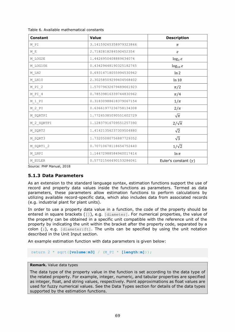
69
Table 6. Available mathematical constants
Constant Value Description
M_PI 3.14159265358979323846 𝜋
M_E 2.7182818284590452354 𝑒
M_LOG2E 1.4426950408889634074 log2 𝑒
M_LOG10E 0.43429448190325182765 log10 𝑒
M_LN2 0.69314718055994530942 ln 2
M_LN10 2.30258509299404568402 ln 10
M_PI_2 1.57079632679489661923 𝜋 2⁄
M_PI_4 0.78539816339744830962 𝜋 4⁄
M_1_PI 0.31830988618379067154 1 𝜋⁄
M_2_PI 0.63661977236758134308 2 𝜋⁄
M_SQRTPI 1.77245385090551602729 √𝜋
M_2_SQRTPI 1.12837916709551257390 2 √𝜋⁄
M_SQRT2 1.41421356237309504880 √2
M_SQRT3 1.73205080756887729352 √3
M_SQRT1_2 0.70710678118654752440 1 √2⁄
M_LNPI 1.14472988584940017414 ln 𝜋
M_EULER 0.57721566490153286061 Euler's constant (𝛾)
Source: PHP Manual, 2018
5.1.3 Data Parameters
As an extension to the standard language syntax, estimation functions support the use of
record and property data values inside the functions as parameters. Termed as data
parameters, these parameters allow estimation functions to perform calculations by
utilizing available record-specific data, which also includes data from associated records
(e.g. industrial plant for plant units).
In order to use a property data value in a function, the code of the property should be
entered in square brackets ([]), e.g. [diameter]. For numerical properties, the value of
the property can be obtained in a specific unit compatible with the reference unit of the
property by indicating the unit within the bracket after the property code, separated by a
colon (:), e.g. [diameter:ft]. The units can be specified by using the unit notation
described in the Unit Input section.
An example estimation function with data parameters is given below:
return 2 * sqrt([volume:m3] / (M_PI * [length:m]));
Remark. Value data types
The data type of the property value in the function is set according to the data type of
the related property. For example, integer, numeric, and tabular properties are specified
as integer, float, and string values, respectively. Point approximations as float values are
used for fuzzy numerical values. See the Data Types section for details of the data types
supported by the estimation functions.

70
Similar to the property data values, record data values (e.g. name) can also be utilized in
the estimation functions. For this purpose, the name token of the record data field prefixed
with exclamation mark (!) should be specified inside the square brackets instead of the
property code, e.g. [!name]. The data types of the record data values are determined
according to their native data type used for the storage in the database.
Remark. Constant values
Values of data parameters are considered to be constant within an estimation function.
Therefore, they cannot be modified.
5.1.4 Operators
An operator takes one or more values or expressions (i.e. statements) and yields another
value. There are unary operators that take only one value, binary operators that take two
values, and a ternary operator that takes three values.
The supported operators are listed in Table 7. The list is not exhaustive and only includes
the operators useful for the estimation functions. See the PHP Manual for the complete list
of operators.
Table 7. Supported operators
Operator Example Name Operator Example Name
= $a = $b Assignment Logical operators
Bitwise operators ! ! $a Not
& $a & $b And && $a && $b And
| $a | $b Or (inclusive or) || $a || $b Or
^ $a ^ $b Xor (exclusive or) Increment/decrement operators
~ ~ $a Not ++ ++$a Pre-increment
<< $a << $b Shift left ++ $a++ Post-increment
>> $a >> $b Shift right -- --$a Pre-decrement
Arithmetic operators -- $a-- Post-decrement
- -$a Negation Comparison operators
- $a - $b Subtraction == $a == $b Equal
+ $a + $b Addition === $a === $b Identical
* $a * $b Multiplication != $a != $b Not equal
/ $a / $b Division <> $a <> $b Not equal
% $a % $b Modulus !== $a !== $b Not identical
** $a ** $b Exponentiation < $a < $b Less than
String operators > $a > $b Greater than
. $a . $b Concatenation <= $a <= $b Less than or equal to
.= $a .= $b Concatenating
assignment
>= $a >= $b Greater than or equal
to
Source: PHP Manual, 2018

71
The precedence of an operator determines how it binds two values or expressions together.
For example, the expression 1 + 2 * 3 evaluates to 7 and not 9 because the precedence
of the multiplication operator (*) is higher than the addition operator (+). Parentheses may
be used to force precedence wherever necessary. For example, (1 + 2) * 3 evaluates to
9. Table 8 lists the supported operators in the order of precedence with associativity
information. Operators listed on the same row have equal precedence.
Table 8. Precedence and associativity of the supported operators
Operators Associativity
** right
++ -- (int) (float) (string) (array) (bool) right
! right
* / % left
+ - . left
<< >> left
< <= > >= none
== != === !== <> none
& left
^ left
| left
&& left
|| left
? : left
= += -= *= **= /= .= %= &= |= ^= <<= >>= => right
Source: PHP Manual, 2018
When operators have equal precedence their associativity decides how the operators are
grouped. For example, 1 * 2 / 3 is grouped as (1 * 2) / 3, because multiplication (*)
and division (/) operators are left-associative. On the other hand, assignment operators
are right-associative and $a = $b = $c is grouped as $a = ($b = $c). Non-associative
operators that have equal precedence cannot be used next to each other, for example
1 < 2 > 1 is not a valid expression.
Hint. Use of parentheses
Use of parentheses is highly recommended as it can prevent potential errors and increase
code readability by making grouping explicit rather than implicit by operator precedence
and associativity.
5.1.5 Variables
Variables, which keep values that are not constant (i.e. can be changed during the
execution of the function) are represented by a dollar sign ($) followed by the name of the
variable. A valid variable name should begin with a letter or underscore, followed by a
series of letters, numbers, or underscores. It is not necessary to initialize variables. Data
types of the variables are also not specified, as the language is capable of determining the
data type of variables and does type conversion (i.e. type casting) automatically.

72
Remark. Variable names
The variables names are case-sensitive, e.g. $var and $Var denote different variables.
$var = "variable";
$Var = "another variable";
By default, variables are always assigned by value, i.e. when an expression is assigned to
a variable, the entire value of the original expression is copied into the destination variable.
This means that after assigning one variable's value to another, changing one of those
variables will have no effect on the other.
// Set value of a as 10
$a = 10;
// Set value of b as equal to a (= 10)
$b = $a;
// Change value of a to 20
$a = 20;
// Value of b is still 10
5.2 Data Types
Variables that are used in an estimation function can store values in various data types.
Although there are some similarities, variable data types are different from the property
data types of the system which are described in the Properties section. The following data
types are supported:
5.2.1 boolean
A boolean expresses a binary value, which can be either TRUE or FALSE.
$val = TRUE;
$val = FALSE;
5.2.2 integer
An integer expresses a number without a fractional component, i.e. ℤ = {…, -2, -1, 0, 1,
2, …}. They are 32 bits signed values with minimum and maximum values of -2147483647
and 2147483647, respectively. A number beyond these values, including one originating
from an expression, is interpreted as a float.
$val = 123;
$val = -123;
5.2.3 float
A float expresses a number with decimal points, e.g. 1.2345. Float values can be assigned
by using the decimal or scientific syntaxes:

73
$val = 1.23;
$val = 1.23e3;
$val = -6.5E-10;
A float approximates a real number by using a fixed number of significant digits that are
scaled using an exponent in base 2. Therefore it has limited precision. The IEEE 754 double
precision format is used internally by PHP, which gives a maximum relative error due to
rounding in the order of 1.11-16. Moreover, rational numbers that are exactly representable
as floating point numbers in base 10 (e.g. 0.1) do not have an exact representation in
base 2. Therefore, results involving floats should not be trusted to the last digit and they
should not be directly used for comparison. For example, the following expression
evaluates to FALSE instead of TRUE as expected normally due to the base 2 rounding:
$sum = 0.1 + 0.2;
$equal = ($sum == 0.3);
In order to test the equality of two float numbers, a custom relative error value that is
acceptable for the calculation should be used. For example, the previous comparison can
be done properly by using the subtraction operator (-) and the absolute value function
abs() as follows, which evaluates to TRUE:
$sum = 0.1 + 0.2;
$equal = (abs($sum – 0.3) < 1e-10);
Some numeric operations can result in an undefined or unpresentable value, which is
denoted by the constant NAN. Such results should be checked by using is_nan() function:
$div = 0 / 0;
if (is_nan($div)) $msg = "not a number"; else $msg = "a number";
5.2.4 string
A string expresses a series of characters in quotation marks (""), which is usually used to
denote text messages. Single quotations ('') can be used to define strings containing
quotation marks.
$text = "This is a string";
$text = 'This is another text with "quotes"';
5.2.5 array
An array expresses a series of other values, which may include values having data types
of null, boolean, integer, float, string, or even nested arrays. Array elements are defined
between square brackets ([]) and separated by commas (,). Both sequential and
associative (i.e. composed of key and value pairs) arrays are supported. For associative
arrays, => operator is used to indicate the value of a key:

74
// Sequential array
$list = [1, 2, 3, 4, 5];
// Sequential array with mixed data type elements
$list = ["A", 1, 'B', 1.23, NULL, [1, 2, 3]];
// Associative array
$list = ["A" => "AA", "B" => "BB", "C" => "CC"];
5.2.6 null
The special NULL value represents a variable with no value. A variable which has not been
set to any value or explicitly set to the constant NULL is considered to be null.
$val = NULL;
5.3 Control Structures
Various control statements (i.e. structures), which allow branching or selective execution
of the statements are supported in the estimation functions.
5.3.1 if … else if … else
if (expr)
statement
else if (expr)
statement
⋮
else
statement
The if … else if… else … statement allows conditional execution of statements. The
expression following the if keyword is evaluated to its boolean value and if it is TRUE, then
the subsequent statement is executed. For example, the following if statement assigns a
value to $msg, if $val is bigger than $otherVal:
if ($val > $otherVal) $msg = "value is bigger than other value";
In order to execute another statement when the expression of the if statement evaluates
to FALSE, the related statement can be specified after the else keyword:
if ($val > $otherVal) {
$msg = "value is bigger than other value";
}
else {
$msg = "other value is bigger than or equal to value";
}
The else if keyword can be used to write successive if statements, which should be
evaluated only if the previous if statement is FALSE:

75
if ($val > $otherVal) {
$msg = "value is bigger than other value";
}
else if ($val < $otherVal){
$msg = "other value is bigger than value";
}
else {
$msg = "value and other value are equal";
}
5.3.2 switch
switch (expr)
case val1:
statement
case val2:
statement
⋮
default:
statement
The switch statement can be used to compare the same expression with multiple values
and evaluate the statement related to the value it equals to. It is like a series of if
statements, but the expression used for the comparison is only evaluated once and it also
allows other applications, such as branching and partial evaluation of the statements by
using selective use of the break and continue keywords. More detailed information on the
switch statement can be found in the PHP Manual.
switch ($val) {
case 1:
$msg = "value is one";
break;
case 2:
$msg = "value is two";
break;
default:
$msg = "value is unknown";
break;
}
5.4 Loops
Various loop statements are available for executing expressions and statements multiple
times, altering some variables if it is necessary.
5.4.1 while
while (expr)
statement

76
while executes the statement as long as the expression evaluates to TRUE at the beginning
of each iteration. If the expression evaluates to FALSE at the very beginning, the statement
is not executed at all. The following function returns the sum of the values between 1 and
9 (inclusive), which is 45.
while ($val < 10) {
$sum += $val;
$val++;
}
return $val;
5.4.2 do … while
do
statement
while (expr)
do … while is similar to while, but the expression is evaluated at the end of each iteration;
hence, the statement is executed at least once. The following function is identical to the
while function given previously:
do {
$sum += $val;
$val++;
} while ($val < 10);
return $val;
The loop below would run only once, because after the first iteration the expression
evaluates to FALSE. Therefore the $sum will be equal to $val, which is 5. A similar while
loop will leave $sum with no value, because the check will be done at the beginning.
$val = 5;
do {
$sum += $val;
} while ($val > 10);
5.4.3 for
for (expr1; expr2; expr3)
statement
The for loop is composed of three expressions and a statement. The first expression is
evaluated at the very beginning, which is usually used to initialize the variables used in the
loop. The second expression is evaluated at the beginning of each iteration. If it evaluates
to FALSE, the loop is terminated. Otherwise, the statement is executed, which is followed
by the evaluation of the third expression at the end of the iteration. The following function
loops through the numbers 1 to 9 and returns the sum:

77
for ($val = 1; $val < 10; $val++) {
$sum += $val;
}
return $sum;
Each expression can be left empty or contain multiple expressions separated by commas.
If the second expression is empty, its value is considered as TRUE; hence, the loop
continues infinitely.
5.4.4 foreach
foreach (array as $val) foreach (array as $key => $val)
statement statement
The foreach loop provides a simple mechanism to iterate over arrays, either providing
value or key and value pair at each iteration evaluating the statement and advancing to
the next item in the array until reaching the end of the array.
$list = [1, 3, 5, 7, 9]; $list = [1, 3, 5, 7, 9];
foreach ($list as $val) { foreach ($list as $key => $val) {
$sum += $val; $sum += $key * $val;
} }
// Returns 25 // Returns 70
return $sum; return $sum;
5.4.5 Nested Loops
Loops can be nested if required:
// First loop
for ($i = 1; $i < 10; $i++) {
// Second loop
for ($j = 1; $j < 10; $j++) {
$sum += $i * $j;
}
}
// Returns 2025
return $sum;
5.4.6 Controlling Loops
Execution of a loop can be terminated by using the break keyword. The following infinite
loop terminates when the sum exceeds 100:
for ($num = 1; ; $num++) {
$sum += $num;
if ($sum > 100) break;
}
return $sum;

78
If more than one loop should be terminated within nested loops, a numeric argument can
be specified to indicate the number of loops to be terminated. The following infinite loop
terminates when the sum exceeds 1,000:
for ($i = 1; $i < 10; $i++) {
for ($j = 1; $j < 10; $j++) {
$sum += $i * $j;
if ($sum > 1000) break 2;
}
}
return $sum;
In the above example, use of the break keyword without 2 will only break the nested loop.
Hence, the outside loop will continue to iterate although the sum is greater than 1,000,
which is not the intended behaviour.
In order to skip to the next iteration without terminating the loop, but only skipping the
execution of the rest of the statements in the loop, the continue keyword can be utilized.
Similar to break, the number of loops to be skipped can be indicated. The following function
returns the sum of a range of numbers, except the even values:
for ($num = 1; $num < 20; $num++) {
if ($num % 2 == 0) continue;
$sum += $num;
}
return $sum;
5.5 Functions
function name(arguments) {
statement
}
Functions allow performing repetitive tasks or calculations, which are based on values of
some variables. In RAPID-N, each estimation function is itself a function, which is
dynamically generated on demand by the data estimation framework. Following the
distributed and atomic logic of the framework, it is good practice to define a custom
estimator whenever there is a need for a computation function to perform a specific
computation. However, in some cases it might be necessary to perform repetitive
calculations inside an estimation function (e.g. root finding, matrix operations,
time-dependant analysis, etc.) which cannot be done by simple looping statements. For
such cases, it is possible to define a custom function using the function syntax.
Information is passed to functions via the argument list (i.e. arguments), which is a
comma-delimited list of expressions. The arguments are evaluated from left to right and
by default passed by value. Variable-length argument lists, default argument values, and
passing arguments by reference are also supported by PHP, details of which can be found
in the PHP Manual.
Functions may contain any valid code statements, including control structures, loops, and
nested functions. Function names follow the same rules as variables, but they are not case
sensitive. Therefore, foo() and Foo() refer to the same function.

79
Remark. Function overloading
Function overloading is not supported, i.e. it is not possible to redefine previously
declared functions. Hence, it is necessary to choose a unique name for a custom function.
As good practice, it is suggested to name custom functions starting with an underscore
(_) and the name of the property that is estimated, followed by a unique name specific
to the estimator (e.g. _volumeIterate).
Similar to the embracing estimation function, the result of the custom function can be
returned by the return keyword. An example estimator with a custom function is given
below, which calculates the sum of squares of number between 1 and 10 (exclusive):
function _square($val) {
return $val * $val;
}
for ($num = 1; $num < 10; $num++) {
$sum += _square($num);
}
return $sum;
Remark. Recursive functions
It is possible to call functions recursively. But calls with over 100-200 recursion levels
should be avoided as it can crash the stack and cause a termination of the data estimation
framework.
5.6 Example Estimation Functions
Example estimation functions, illustrating the syntax and the features of the programming
language, as extended by the data estimation framework are given below:
Function 1. Endpoint distance for confined vapour cloud explosion (Multi-energy model)
// Calculate energy of blast (3.5 Mj/m3 = average for most hydrocarbons)
$E = [VCVo:m3] * 3.5e6;
// Calculate scaled pressure
$Ps1 = [ePd:Pa] / [PA:Pa];
// Calculate scaled distance (for class 10)
$r1 = max(0.4096 * pow($Ps1, -0.859), 0.6829 * pow($Ps1, -0.414));
// Calculate explosion radius
$r = $r1 * pow($E / [PA:Pa], 1/3);
// Return distance in m
return $r;

80
Function 2. Storage height from storage volume and diameter for spherical plant units
// Return zero if stored volume is zero
if (\Scientific::equals([VST:m3], 0)) return 0.0;
// Return unit height if stored volume equals unit volume
if (\Scientific::equals([VST:m3], [V:m3])) return [D:m];
// Solve by Newton's rule
$x = [D:m] / 2;
while (TRUE) {
$y = M_PI * $x * $x * ([D:m] / 2 - $x / 3) - [VST:m3];
if (\Scientific::equals($y, 0)) return $x;
$x = $x - $y / (M_PI * $x * ([D:m] - $x));
}
Function 3. Flame tilt angle from Froude and Reynolds numbers (TNO method)
// Kinematic viscosity of air (m2/s, at 300K)
$v = 1.568e-5;
// Froude number
$Fr = pow([u:m/s], 2) / (9.80665 * [DP:m]);
// Reynolds number
$Re = [u:m/s] * [DP:m] / $v;
// tan(theta) / cos(theta)
$c = 2/3 * pow($Fr, 1/3) * pow($Re, 0.117);
// Theta (rad)
$theta = asin((pow(4 * pow($c, 2) + 1, 0.5) - 1) / (2 * $c));
// Return tilt angle in degrees
return rad2deg($theta);

81
6 Tutorials
In order to demonstrate data entry and analysis steps that should be followed to perform
Natech risk analysis in RAPID-N, several tutorials are provided in this section. The tutorials
start with data entry for the basic records required for the risk analysis (i.e. natural hazard
event, industrial plants, and plant units) and followed by risk analyses ranging from an
analysis involving a single plant to an analysis involving multiple plants and plant units.
Some steps which are identical in the tutorials are described in detail in the first tutorial
involving the step, but they are also usually repeated in the subsequent tutorials so that
each tutorial can be used separately. Still, it is suggested to follow the tutorials in the given
order.
6.1 Creating Natural Hazard Data
RAPID-N provides an extensive database of past earthquakes, which is publicly available
for Natech risk analysis. However, frequently it is also necessary to define case-specific
natural hazard scenarios, which are not limited to historical events and earthquakes. This
tutorial demonstrates how a natural hazard event scenario can be entered into the system.
The described hazard event is used for the risk analysis tutorials, which are provided in the
following sections.
The Hazards listing page, which is accessible through the home or personal pages, or the
bottom directory available at each page, lists the available natural hazard records in the
system. By clicking on the "Create" button on the listing page you can access the Create
Hazard page, which displays the natural hazard data entry form. You can also use the
following link: http://rapidn.jrc.ec.europa.eu/hazard/create.
Remark. Access to the "Create Hazard" page
Because only registered users are allowed to create new records, the "Create" button
and the "Create Hazard" page are only available if you sign-in to the system. See User
Access and Data Access sections for more details.
The natural hazard data entry form is composed of a map from which you can set the
geographic location and extent of the natural hazard event, and a series of input elements
through which you can enter natural hazard event data.
Detailed information on hazard records is given in the Hazards section. An example data
entry form is given in Figure 32, which includes the data that will be entered throughout
the tutorial. At the end of the tutorial your data entry form should be in a similar state;
therefore, you can use the figure to check and validate your data entry steps.

82
Figure 32. Natural hazard data entry form of the tutorial hazard
Source: JRC, 2018

83
For the tutorial, please follow the following steps:
1. Specify the name of the natural hazard event in the Name text input field. For this
tutorial, we will use "Tutorial Hazard". If you want you can also indicate another name.
Type the name in the input field.
2. Select the type of the natural hazard (e.g. earthquake, flood, landslide, etc.) by using
the Type drop-down list. Select the "Earthquake" option.
3. Enter the date of the event in the Date input field. You can either type the date or
choose it from the calendar window by clicking on the "Calendar" icon located at the
end of the input field. Select today as the date.
Remark. Time zone
The date should be in the Coordinated Universal Time (UTC). See the Unit Input
section for more details on the date inputs.
4. Specify the country of origin by choosing a country from the Country drop-down list.
Select "Italy".
5. In addition to the country, the province of the origin can also be indicated by using the
Province text input field. Because it is not mandatory, leave it empty.
6. You can indicate the coordinates of the origin of the natural hazard event in the
Coordinates input field. You can manually enter the coordinates or select a point on the
map, which is located at the top of the data entry form. If you click on a location on
the map, a point will be displayed and its coordinates will be automatically entered to
the Coordinates input field. You can change the coordinates manually by entering new
latitude and longitude values, or by dragging and dropping the point on the map to
another location. See the Mapping section for a detailed description on how to edit
features on the map. For this tutorial, enter 46.2661894 as latitude and 8.3528003 as
longitude manually.
Remark. Coordinate format
In addition to the decimal degrees format (e.g. 45.5084), you can also enter the
coordinates manually in degrees decimal minutes (e.g. 45 30.504) or degrees
minutes seconds (e.g. 45 30 30.24) formats. See the Data Entry Maps section for
more details.
7. From the Hazard Map drop-down list, you can specify the default hazard map of the
event, which is by default utilized by the system for the calculation of on-site hazard
parameters as indicated in the Hazards section. The drop-down list only displays the
hazard maps available in the system that are linked to the natural hazard event.
Because the natural hazard event does not exist yet (i.e. has not been created), there
are no hazard maps available; hence, the list is empty. Select "None".
8. By using the Hazard Parameters input, you can enter the parameters describing the
source characteristics of the natural hazard event. Initially, the "No hazard parameters"
message will be displayed with an "Add" button indicated by a plus icon. By clicking on
the "Add" button you can add a new parameter data row to the hazard parameters list.
According to the hazard type selected in the Type drop-down list, the related properties
available in the system will be listed in the Property drop-down list of the row. Once
you choose a property, additional input elements will be displayed in the same row for
the entry of the parameter value. You can specify the value and other related
information (e.g. measurement unit) of the parameter by using these input elements.
By clicking the "Remove" button indicated by a minus icon you can remove the
parameter data row from the list, or by clicking the "Add" button again you can add a
new parameter data row. See the Properties Input section for the details of property
data entry.

84
For this tutorial, you will add two hazard parameters:
(a) For the first parameter, click on the "Add" button and select the "Moment
Magnitude" property from the list which will be displayed in a new row. Once you
select the property, a numerical value entry input, which supports fuzzy numbers,
will be displayed in the same row. Enter 6.5 as the value.
(b) For the second parameter, click on the "Add" button displayed on the "Moment
Magnitude" row. A new row will be added to the list. Select the "Focal Depth"
property in the new row. Once you select the property, besides a numerical value
entry input similar to the first parameter, a unit input will also be displayed because
focal depth is a numerical property with a reference unit of kilometre. Enter 10 as
the value and km as the unit.
Hint. Search box
You can use the inline search box of the property drop-down list to filter the available
properties and select the property that you want quickly.
Remark. Available properties
A full listing of the properties with their data types and related reference units is
available at the Properties listing page. To quickly access the listing page, you can
use the following link: http://rapidn.jrc.ec.europa.eu/property/list.
9. You can specify some notes or remarks about the natural hazard event by using the
Notes wiki input field. See the Wiki Input section for more details on wiki inputs, which
support formatted output, including emphasis, subscript, superscript, sorted and
unsorted lists, and links. For this tutorial, leave it empty.
10. Specify the access level of the natural hazard record by selecting a state from the
Access drop-down list. Select "Private", which makes the record available only to you.
See the Data Access section for a detailed description of the available states and the
access control mechanism of the system.
After all the input data has been entered, click on the "Create" button to complete data
entry and save the natural hazard record in the system. The Create Hazard page will be
closed and replaced with the Hazard page, which will display the record information and
provide access to associated actions, such as updating or deleting of the record, or creating
related records such as hazard maps, on-site hazard data, and risk analyses. The page
should be similar to the one given in Figure 33.
Besides the data that you entered, you will also see additional data related to the event
that is obtained by the system automatically by using the data estimation framework. The
estimated data is shown together with the user-defined data, but highlighted in red (Figure
33). By hovering the mouse pointer over the estimated value you can see how the data
was estimated (i.e. which property estimator is utilized). Also by clicking on the value, you
can access to the Property Estimator information page of the associated estimator which
provides detailed data on the estimation method. See the Data Estimation Framework
section for more details on the data estimation capabilities of RAPID-N.

85
Figure 33. Natural hazard information page of the tutorial hazard
Source: JRC, 2018

86
6.2 Creating Industrial Plant and Plant Unit Data
RAPID-N requires data on the hazardous installations to analyse the Natech risk. This
includes information related to the hazardous materials and the plant units. Thus, it is
necessary to define case-specific industrial data. This tutorial demonstrates how to create
an industrial plant record and how to add the information on plant units located at the
plant. The described industrial plant and plant units are used for the risk analysis tutorials
provided in the following sections.
6.2.1 Industrial Plant
The Industrial Plants listing page, which is accessible through the home or personal pages,
or is available from the bottom directory at each page, lists the available industrial plant
records in the system. By clicking on the "Create" button on the listing page, you can
access the Create Industrial Plant page, which displays the industrial plant data entry form.
You can also use the following link: http://rapidn.jrc.ec.europa.eu/plant/create.
The Industrial plant data entry form is composed of a map, from which you can set the
geographic location and draw the boundaries of the industrial plant, and a series of input
elements through which you can enter industrial plant data.
Detailed information industrial plant records is given in the Industrial Plants section. An
example industrial plant data entry form is given in Figure 34, which includes the data that
will be entered throughout the tutorial. At the end of the tutorial your data entry form
should be in a similar state; therefore, you can use the figure to check and validate your
data entry steps.

87
Figure 34. Industrial plant data entry form of the tutorial plant
Source: JRC, 2018
88
For the tutorial, please follow these steps:
1. Specify the name of the industrial plant in the Name text input field. For this tutorial,
we will use "Tutorial Plant A". If you want, you can indicate another name. Type the
name in the input field.
2. The operator of the plant can be selected by pressing "Select" button in the Operator
input field and selecting an operator from the Operators listing page which will be
opened. Because it is not mandatory, leave it empty.
3. Specify the country of the plant by choosing a country from the Country drop-down
list. Select "Italy".
4. The province of the plant can be indicated by using the Province text input field.
Because it is not mandatory, leave it empty.
5. The city of the plant can be indicated by using the City text input field. Type the city
name "Ispra".
6. The address can also be indicated by using the Address text input field. Because it is
not mandatory, leave it empty.
7. You can indicate the coordinates of the industrial plant in the Coordinates input field.
You can manually enter the coordinates or select a point on the map, which is located
at the top of the data entry form. For this tutorial, enter 45.8095019 as latitude and
8.6319478 as longitude. The map at the top of the page will automatically zoom on the
industrial plant area. A white point and a toolbar will be displayed on the map at the
specified location.
You can use the map toolbar to delineate the industrial plant boundaries. Click on the
"Create Geometry" button indicated by a rectangle icon to generate a polygon on the
map. Drag and drop the polygon edges to change the polygon shape, so that it mirrors
the polygon on Figure 34. See the Mapping section for a detailed description on how to
edit features on the map.
8. By using the Properties input, you can enter the parameters describing the
characteristics of the industrial plant. Initially, the "No plant properties" message will
be displayed with an "Add" button indicated by a plus icon. By clicking on the "Add"
button you can add a new parameter data row to the properties list. Once you choose
a property, additional input elements will be displayed in the same row for the entry of
the parameter value. You can specify the value and other related information (e.g.
measurement unit) of the parameter by using these input elements. By clicking the
"Remove" button, indicated by a minus icon, you can remove the parameter from the
list, or by clicking the "Add" button again you can add a new parameter. See the
Properties Input section for the details of property data entry.
For this tutorial, you will add one property:
Click on the "Add" button and select the "Year of Construction" property from the list.
Once you select the property, a numerical value entry input will be displayed. Enter
2000 as the value.
Hint. Search box
You can use the inline search box of the property drop-down list to filter the available
properties and select the property that you want quickly.
Remark. List of properties
A full listing of the properties with their data types and related reference units is
available at the Properties listing page. To quickly access the listing page, you can
use the following link: http://rapidn.jrc.ec.europa.eu/property/list.

89
9. You can specify some notes or remarks about the industrial plant by using the Notes
wiki input field. See the Wiki Input section for more details on wiki inputs, which support
formatted output, including emphasis, subscript, superscript, sorted and unsorted lists,
and links. For this tutorial, leave it empty.
After all the input data has been entered, click on the "Create" button to complete data
entry and save the industrial plant record in the system. The Create Industrial Plant page
will be closed and replaced with the Industrial Plant page, which will display the record
information and provide access to associated actions, such as updating or deleting of the
record, or creating related records (i.e. plant units, on-site hazard data, Natechs and risk
analyses). The page should look similar to the one given in Figure 35.
Besides the data that you entered, you will also see additional data related to the event
that is obtained by the system automatically by using the data estimation framework. The
estimated data is shown together with the user-defined data, but highlighted in red (Figure
35). By hovering the mouse pointer over the estimated value you can see how the data
was estimated (i.e. which property estimator is utilized). By clicking on the value, you can
access to the Property Estimator information page of the related estimator which provides
detailed data on the estimation method. See the Data Estimation Framework section for
more details on the data estimation capabilities of the system. The map shows the
industrial plant location and boundaries in a vivid green, while plant units are depicted in
red. At this point, you should not be able to see any red polygons at the plant.
Remark. Other industrial plants
Other industrial plants may be present in the same area shown by the map. They are
also reported, as well as their boundaries, in a paler shade of green compared to the
current industrial plant.

90
Figure 35. Industrial plant information page of the tutorial plant
Source: JRC, 2018

91
6.2.2 Plant Units
You can add plant units to the current industrial plant record directly from the Industrial
Plant page. Initially, the "No plant units" message will be displayed under the Plant Units
section. By clicking on the "Create" button under the Plant Units section, you can access
the Create Plant Unit page, which displays the plant unit data entry form. The industrial
plant of the unit will be set automatically.
The plant unit data entry form is composed of a map, from which you can view the
associated industrial plant boundaries and draw the shape of the plant unit, and a series
of input elements through which you can enter plant unit data.
Detailed information on plant unit records is given in the Plant Units section. An example
plant unit data entry form is given in Figure 36, which includes the data that will be entered
throughout the tutorial for one of the plant units. At the end of the tutorial your data entry
form should be in a similar state; therefore, you can use the figure to check and validate
your data entry steps.

92
Figure 36. Plant unit data entry form of the tutorial plant unit
Source: JRC, 2018

93
For this tutorial, you will add two plant units: one atmospheric storage tank containing
diesel fuel and one stack.
For the data entry of the first unit, please follow these steps:
1. Select the type of the plant unit (e.g. storage tank, reactor, pump, etc.) by using the
Type drop-down list. Select the "Storage Tank" option.
2. Specify a code for the plant unit in the Code text input field. For this tutorial, we will
use "Atm_St_TK". If you want, you can indicate another code. Type the code in the
input field.
3. On the map located at the top of the page, click at the centre of the big tank within the
facility boundaries to set the plant unit coordinates. A white point and a toolbar will be
displayed on the map at the clicked location. The Coordinate text input fields will be
automatically filled. See the Mapping section for a detailed description on how to edit
features on the map.
4. The substance can be indicated by pressing "Select" button in the Substance input field
to open the Substances listing page. Search the substance by using the provided filters
as described in the Data Query and Listing section and select "Diesel Fuel No.2" from
the substance list. You can use Diesel as the keyword to find it quickly.
5. By using the Properties input, you can enter the characteristic parameters of the plant
unit. Initially, the "No plant unit properties" message will be displayed with an "Add"
button indicated by a plus icon. By clicking on the "Add" button you can add a new
parameter data row to the properties list. According to the plant unit type selected in
the Type drop-down list, the related properties available in the system will be listed in
the row. Once you choose a property, additional input elements will be displayed in the
same row for the entry of the parameter value. You can specify the value and other
related information (e.g. measurement unit) of the parameter by using these input
elements. By clicking the "Remove" button, indicated by a minus icon, you can remove
the parameter from the list, or by clicking the "Add" button again you can add a new
parameter. See the Properties Input section for the details of property data entry.
For this unit, you will add five properties:
(a) Click on the "Add" button and select the "Shape" property from the list. Once you
select the property, a drop-down entry input will be displayed. Select the option
"Cylindrical Vertical".
(b) Click on the "Add" button and select the "Base Support Type" property from the list.
Once you select the property, a drop-down entry input will be displayed. Select the
option "Unanchored".
(c) Click on the "Add" button and select the "Roof Type" property from the list. Once
you select the property, a drop-down entry input will be displayed. Select the option
"Fixed Roof".
(d) Click on the "Add" button and select the "Base Type" property from the list. Once
you select the property, a drop-down entry input will be displayed. Select the option
"On-ground".
(e) Click on the "Add" button and select the "Diameter" property from the list. Once
you select the property, a numerical value entry input (which supports fuzzy
numbers) and a unit input will be displayed. Enter "28" as the value and "m" as
the unit. A circle is automatically drawn on the map around the plant unit location,
matching the given diameter.
Hint. Search box
You can use the inline search box of the property drop-down list to filter the available
properties and select the property that you want quickly.

94
Remark. List of properties
A full listing of the properties with their data types and related reference units is
available at the Properties listing page. To quickly access the listing page, you can
use the following link: http://rapidn.jrc.ec.europa.eu/property/list.
6. You can use the map toolbar on the map to modify the plant unit shape and ensure a
perfect fit with the satellite image. You can drag and drop at any point inside the circle
to move it. You can also drag and drop the points displayed on the circle to change its
size (i.e. diameter). See the Mapping section for a detailed description on how to edit
features on the map.
7. You can specify some notes or remarks about the plant unit by using the Notes wiki
input field. See the Wiki Input section for more details on wiki inputs, which support
formatted output, including emphasis, subscript, superscript, sorted and unsorted lists,
and links. For this tutorial, leave it empty.
After all the input data has been entered, click on the "Create" button to complete data
entry and save the plant unit record in the system. The Create Plant Unit page will be
closed and replaced with the Industrial Plant page displayed initially. A table listing the
plant units of the plant is now available in the Plant Units section. For the time being, the
table contains only one record row, which describes the plant unit you just created.
For the data entry of the second unit, please follow these steps:
1. Select the type of the plant unit (e.g. storage tank, reactor, pump, etc.) by using the
Type drop-down list. Select the "Stack" option.
2. Specify a code for the plant unit in the Code text input field. For this tutorial, we will
use "Stk". If you want, you can indicate another name. Type the name in the input
field.
3. Click at the base of the chimney within the facility boundaries to set the plant unit
coordinates. A white point and a toolbar will be displayed on the map at the coordinate
location. The Coordinate text input fields will be automatically filled.
4. The substance can be indicated by pressing "Select" button in the Substance input field,
to open the Substances listing page. Because the stack is not supposed to contain any
hazardous material, leave it empty.
5. By using the Properties input, you can enter the parameters describing the
characteristics of the plant unit as you did for the first plant unit before.
For this unit, you will add two properties:
(a) Click on the "Add" button and select the "Shape" property from the list. Once you
select the property, a drop-down entry input will be displayed. Select the option
"Cylindrical Vertical".
(b) Click on the "Add" button and select the "Diameter" property from the list. Once
you select the property, a numerical value entry input (which supports fuzzy
numbers) and a unit input will be displayed. Enter "5" as the value and "m" as the
unit. A circle is automatically drawn around the unit coordinate, matching the given
diameter.
6. You can use the map toolbar on the map to modify the plant unit shape and ensure a
perfect fit with the satellite image as you did for the first plant unit.
7. You can specify some notes or remarks about the plant unit by using the Notes wiki
input field. For this tutorial, leave it empty.
After all the input data has been entered, click on the "Create" button to complete data
entry and save the plant unit record in the system. The Create Plant Unit page will be
closed and replaced with the Industrial Plant page displayed initially. The plant units table
now contains two record rows, which describes the plant units you created in the tutorial.

95
The map view of the plant should also display the two units as shown in Figure 37.
Figure 37. Map of the tutorial plant and plant units
Source: JRC, 2018
If you click on one of the two plant units listed, the system will open the Plant Unit page,
which will display the detailed record information and provide access to associated actions,
such as updating or deleting of the record, or creating related records.
Besides the data that you entered, you will also see additional data related to the selected
plant unit that is obtained by the system automatically by using the data estimation
framework. The estimated data is shown together with the user-defined data, but
highlighted in red (Figure 38). By hovering the mouse pointer over the estimated value
you can see how the data was estimated (i.e. which property estimator is utilized). Also by
clicking on the value, you can access to the Property Estimator information page of the
related estimator which provides detailed data on the estimation method. See the Data
Estimation Framework section for more details on the data estimation capabilities of the
system. The map shows the industrial plant unit location and shape in red.

96
Figure 38. Plant unit information page of the tutorial plant unit
Source: JRC, 2018

97
6.3 Single Plant Natech Risk Analysis
A risk analysis study involving a single plant can be a useful tool for plant operators and
engineering companies to identify Natech hazards and quantify Natech risks. It can be also
useful for public authorities that want to investigate the Natech risks of a hazardous
installation in their territory.
In this tutorial, you will learn the basics of Natech risk analysis by using RAPID-N and
following a step-by-step guided procedure. All the resources needed for this exercise are
publicly available in RAPID-N and are composed of a fictional natural hazard event named
"Tutorial Hazard", which is created in the first tutorial, and a fictional industrial plant named
"Tutorial Plant A", which is created in the second tutorial. Completed risk analysis is also
available publicly as "Tutorial Risk Analysis 1". You can find detailed information on the
risk analysis methodology of RAPID-N in the Risk Analysis Methodology section.
6.3.1 Data Entry
The risk analysis data entry form is composed of a series of input elements through which
you can enter risk analysis information and setup risk analysis parameters. Detailed
information on risk analysis records is given in the Risk Analyses section. An example data
entry form is given in Figure 39.
Figure 39. Risk analysis data entry form of the tutorial risk analysis
Source: JRC, 2018

98
For the data entry and analysis, please follow the following steps:
1. From the home or personal pages, click on the "Risk Analyses" icon to access the Risk
Analyses listing page. You can also use the following link to access the listing page
directly: http://rapidn.jrc.ec.europa.eu/risk_analysis/list.
2. Click on the "Create" button in the toolbar to open the Create Risk Analysis page.
3. Choose a name for your risk analysis case-study and type it in the Name input field.
For this tutorial we will use the name "Tutorial Risk Analysis 1".
4. Select a hazard record, which will be used to define the triggering natural hazard event.
Click on the "Select" button in the Hazard input to open the Hazards listing page. Search
for the hazard record named "Tutorial Hazard" and once the search results are
displayed, select it from the listing table by clicking on its name. The hazard record you
selected is the tutorial hazard record that you created previously, which is a scenario
earthquake with a moment magnitude of 6.5 and focal depth of 10 km, having an
epicentre that is approximately 60 km away from the case-study plant.
5. You can choose one of the hazard maps related to the hazard from the Hazard Maps
drop-down list, which will provide pre-calculated on-site hazard parameters for the
analysis. If set as "Default", RAPID-N will use the default hazard map specified in the
hazard record. Leave it as "Default".
Remark. Estimation of on-site hazard parameters
If no default hazard map is specified in the natural hazard record or the "Enable
Hazard Maps" risk analysis property is set as disabled, the system will use other
methods (i.e. on-site hazard data records or data estimation by using property
estimators) to calculate the on-site hazard parameters.
Remark. Use of a hazard map
Use of a hazard map does not limit the calculation of on-site parameters to the
parameters that are available in the hazard map. RAPID-N uses the available
parameters to estimate additional ones by utilizing the data estimation framework.
6. You can choose a specific industrial plant for the analysis or let RAPID-N identify and
consider all the plants located in the natural hazard area. For this tutorial, you must
select a case-study plant. Click on the "Select" button in the Industrial Plant input to
open the Industrial Plants listing page. Search for the industrial plant named "Tutorial
Plant A" and select it from the list by clicking its name.
7. The Create Risk Analysis page should look like the Figure 39 above after the hazard
and the industrial plant are selected. At this point, by clicking the names of the hazard
and industrial plant you can access associated information pages, which provide
detailed information on the hazard and industrial plant, respectively.
8. By using the Plant Unit drop-down list, you can choose whether the analysis should
consider all plant units located at the plant, or should focus only on a specified single
plant unit. For this tutorial, select All.
9. You can specify custom on-site hazard parameters which should be considered for the
analysis by entering them manually in the On-Site Hazard Parameters input. For this
tutorial, do not add any on-site hazard parameters.
10. You can specify Risk Analysis Parameters, which allow you to customize the risk
analysis process. For this tutorial, our aim is to perform a simple risk analysis.
Therefore, we will let RAPID-N use the default parameters by not entering any custom
parameters. Leave the Risk Analysis Parameters input empty.
11. Click on the "Create" button to save the risk analysis record and perform the analysis.

99
RAPID-N will collect all necessary data, estimate missing ones, and assess natural hazard
impact, possible Natech scenarios, and related consequences for the plant units located at
the specified industrial plant. At the end of the analysis, an analysis report and a risk map
will be displayed.
6.3.2 Results
The Tutorial Plant A is a simple plant, which is composed of only two units: an unanchored
atmospheric storage tank and a stack identified as "Atm_St_TK" and "Stk" respectively
(Figure 37). The analysis results are shown on the reference map and on the satellite image
in Figure 40, whereas Figure 41 represents the same results in the detailed tabular form.
For simplicity, the detailed consequence analysis results are shown in the table only for
DS2.
Figure 40. Risk analysis map
Source: JRC, 2018
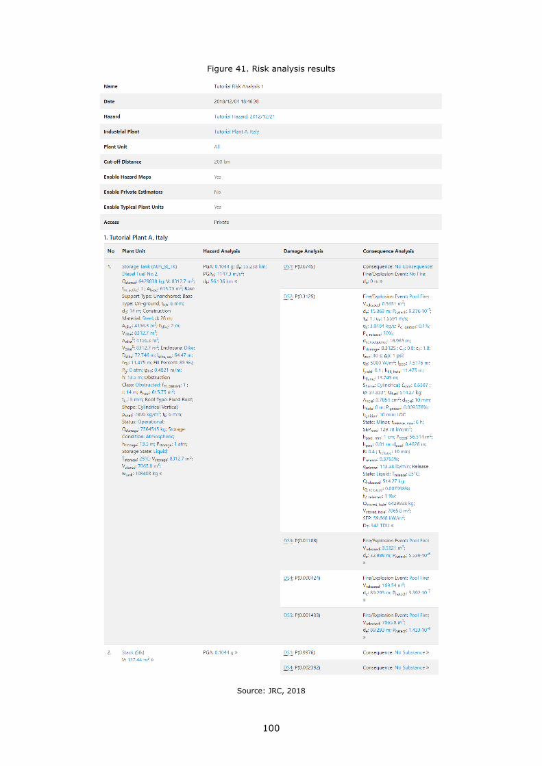
100
Figure 41. Risk analysis results
Source: JRC, 2018

101
Hazard impact/exposure
RAPID-N calculated the earthquake intensity parameters at the plant, more specifically at
the location of the two units. The calculated intensity is expressed as Peak Ground
Acceleration (PGA) and it is equal to 0.1044 g for both units. The intensity is the same for
both units, because they are located next to each other. For units scattered around a large
facility, the results might be different.
Damage assessment
RAPID-N chose a fragility curve for each unit and calculated the probable damage. The
atmospheric storage tank has 5 damage states (DS1: None, DS2: Minor, DS3: Moderate,
DS4: Extensive and DS5: Complete), while the stack has only 2 (DS1: None and DS4:
Extensive).
Damage probability
Based on the fragility curves, for the atmospheric storage tank the probability of damage
is 31% for DS2, about 1.1% for DS3 and much lower for DS4 and DS5. The probability of
damage to the stack is very small (0.2%).
One may conclude that for this hazard scenario minor damage to the tank is likely,
moderate damage is unlikely and extensive or complete damage are extremely rare.
Extensive damage to the stack is also rare.
Consequences
The gravity of the consequences can be directly related to the level of physical damage,
i.e. to the damage state. The higher the damage, the higher the amount of hazardous
substance released. In this case, the amount of fuel (diesel) released varies between
500 kg for minor damage to more than six thousand tons in case of complete damage. As
the fuels and chemicals are often valuable products, their accidental loss is not only a
safety concern but also an immediate cost to the business.
The storage tank shows consequences of the "Pool Fire" type, as it contains a liquid fuel
that may ignite if released. In case the fuel spill ignites, the resulting fire can affect humans
as far as 15.4 m away in case of minor damage and as far as 89 m away in case of complete
damage. Damage classes "Extensive" and "Complete" result in the same end-point
distance, as the size of the fire is supposed to be limited by a containment dike. The values
of the endpoint distances would indeed be different should we remove the containment
dikes.
The stack does not contain any hazardous material. Thus, in case of damage it does not
have any direct consequence aside from the repair/rebuilding costs. However, there were
cases in the past which involved secondary damage to plant units due to impact of
collapsed stacks (Girgin, 2011). Hence, such non-hazardous units might be included into
domino scenarios, especially if the damage probability is high.

102
6.4 Single Plant Natech Risk Analysis with Custom Parameters
In the previous tutorial, on-site hazard intensity parameters were estimated automatically
by RAPID-N by using available property estimators, which correspond to ground motion
prediction equations (GMPE) for earthquakes. However, these parameters can also be
specified manually for the analysis. This tutorial will demonstrate how to customize
natural-hazard related data. A custom Peak Ground Acceleration (PGA) value of 0.15 g will
be used for this purpose.
All the resources needed for this exercise are publicly available in RAPID-N and are
composed of a fictional hazard named "Tutorial Hazard", which was created in the first
tutorial, and a fictional industrial plant named "Tutorial Plant B". Completed risk analysis
is also available publicly as "Tutorial Risk Analysis 2". You can find detailed information on
the risk analysis methodology of RAPID-N in the Risk Analysis Methodology section.
6.4.1 Data Entry
Steps 1-8 are similar to the previous tutorial. Please read the previous tutorial before this
one to obtain more detailed information. Detailed information on risk analysis records is
given in the Risk Analyses section. At the end of the data entry, the risk analysis data entry
form should be similar to Figure 42.
Figure 42. Risk analysis data entry form with custom hazard data
Source: JRC, 2018

103
For the data entry and analysis, please follow the following steps:
1. From the home or personal pages click on the "Risk Analyses" icon to access the Risk
Analyses page.
2. Click on the "Create" button to open the Create Risk Analysis page.
3. Choose a name for your risk analysis and type it in the Name input field. For this
tutorial, we will use "Tutorial Risk Analysis 2".
4. Select the natural hazard scenario by clicking on "Select" button of the Hazard input to
open the Hazards listing page and click on the hazard name on the hazards listing table
after performing a search for "Tutorial Hazard".
5. You can choose a hazard map from the Hazard Map drop-down list or let RAPID-N utilize
the default hazard map of the hazard record, if it is available. Select "Default".
6. You can choose a particular industrial plant for the analysis or let RAPID-N consider all
the plants located in the natural hazard impact area. Select industrial plant named
"Tutorial Plant B" by clicking on the "Select" button of the Industrial Plant input,
performing a search by name, and clicking the name of the plant on the table listing
the search results.
7. At this point, you can click on their names of the hazard and the industrial plant selected
in the Hazard and Industrial Plant inputs to access corresponding information pages,
which provide detailed information.
8. By using the Plant Unit drop-down list, you can choose whether the analysis should
consider all plant units located at the plant, or should focus only on a specified single
plant unit. For this tutorial, select All.
9. You can specify custom on-site hazard parameters which should be considered for the
analysis by entering them manually in the On-Site Hazard Parameters input. For this
tutorial, click on the "Add" button in On-site Hazard Parameters input. Select the
property "Peak Ground Acceleration" from the property drop-down list. Type "0.15" in
the value field and "G" in the unit field.
10. You can specify risk analysis parameters, which allow you to customize the risk analysis
calculations. For this tutorial, leave the Risk Analysis Parameters input empty.
11. Click on the "Create" button to save the risk analysis record and perform the analysis.
6.4.2 Results
The Tutorial Plant B is a more complex plant compared to the Tutorial Plant A. It is divided
into four areas as shown in Figure 43.
The liquid fuel storage area includes four cylindrical vertical atmospheric storage tanks
containing flammable liquids. Two of the storage tanks contain gasoline and are anchored,
while the other two contain diesel and are unanchored. For each couple, one of the storage
tanks is filled to the 45% of its capacity, while the other is filled to 85% of its capacity.
The pressurized fuel storage area contains three horizontal cylindrical tanks with flammable
gases liquefied under pressure. Two tanks contain propane, one of which lies directly on
the ground and the other is on a support. The third tank contains butane and is on a
support.
The water storage area contains three horizontal cylindrical tanks with water at
atmospheric pressure, one of which lies directly on the ground and the other two are on a
support.
The toxic storage area contains two horizontal cylindrical tanks with toxic gases liquefied
under pressure. One tank contains ammonia and is on a support, the other tank contains
chlorine and lies on the ground.

104
Figure 43. Tutorial plant units
Source: JRC, 2018
A summary of the plant units that contains their descriptions is provided in Figure 44.
Figure 44. Details of tutorial plant units
Source: JRC, 2018
For each unit, the same considerations as described in the previous tutorial apply.
However, the results are different due to different physical, operational, and hazardous
characteristics of the units. Since the impact areas are significantly different, some specific
results will be commented for each area separately.

105
Figure 45 reports the result summary for the atmospheric liquid fuel storage area. It is
important to note that RAPID-N selected different fragility curves for each storage tank
depending on their filling level and on their support type (i.e. anchored or unanchored).
For the two tanks with filling level at 45%, RAPID-N selected the same fragility curve, this
means that their damage and Natech probabilities will be identical. However, for the two
other tanks with filling levels at 85%, RAPID-N selected different fragility curves, one for
anchored tanks and the other for unanchored tanks.
Figure 45. Results of the analysis for atmospheric storage tanks
Source: JRC, 2018
Figure 46 reports the summary of the results for the pressurized fuel storage area. Similar
to the atmospheric liquid fuel storage tanks, RAPID-N selected different fragility curves for
each pressurized storage tanks depending on whether they are on the ground or on
supports. For the two tanks on a support (above ground) RAPID-N selected the same
fragility curve, this means that their damage and Natech probabilities will be identical.
However, for the third tank on the ground, RAPID-N was not able to find any fragility curve
and did not assess the damage. This is due to limited knowledge available about
earthquake impact on on-ground pressurized tanks in the scientific and technical literature.
By providing custom fragility damage functions or fragility curves, the users can also
analyse this kind of unit with RAPID-N. The Natech scenario is a Vapour Cloud Explosion,
which may be harmful to humans and to structures up to several hundred meters away.

106
Figure 46. Results of the analysis for pressurised storage tanks
Source: JRC, 2018
Figure 47 reports the result summary for the water storage area. For the two tanks on a
support (above ground) RAPID-N selected the same fragility curve, resulting in identical
damage and Natech probabilities. However, the third tank that is on the ground and
fragility curves are available for on ground atmospheric storage tanks. Therefore, RAPID-N
selected the corresponding fragility curve. In this case, "No consequence" is reported as
water is not a hazardous material.
Figure 47. Analysis results for water storage area
Source: JRC, 2018

107
Figure 48 reports the result summary for the Toxic storage area. For the ammonia tank on
a support (above ground) RAPID-N successfully found and selected one fragility curve,
while for the other tank containing chlorine that is on the ground, RAPID-N was not able
to find any fragility curve and could therefore not assess the damage. In this case the
Natech scenario is not indicated. The release of toxic material to the environment is
dangerous because of the inherent danger posed by the dispersion of toxic vapours in the
air. This scenario is very serious and in case of DS3 (extensive damage), endpoint distances
are of the order of tens of kilometres.
Figure 48. Analysis results for the toxic area
Source: JRC, 2018
Figure 49 reports the results on a map. Endpoint distances are reported as circles around
each unit. Fire and explosion scenarios have red circles, while toxic dispersion scenarios
have orange circles.

108
Figure 49. Risk analysis map
Source: JRC, 2018

109
6.5 Multiple Plant Natech Risk Analysis
A risk analysis study for a hazard scenario involving multiple industrial plants
simultaneously can be useful for public authorities who want to investigate the Natech risks
in an area under their jurisdiction that could include several industrial plants with
hazardous substances. This is an easy and straightforward task with RAPID-N.
All the resources needed for this tutorial exercise are publicly available in RAPID-N and are
composed of a fictional natural hazard event named "Tutorial Hazard", which is created in
the first tutorial, and two fictional industrial installations named "Tutorial Plant A" and
"Tutorial Plant B". Completed risk analysis is also available publicly as "Tutorial Risk
Analysis 3". You can find detailed information on the risk analysis methodology of RAPID-N
in the Risk Analysis Methodology section.
6.5.1 Data Entry
1. From the home or personal pages click on the "Risk Analyses" icon to open the Risk
Analyses listing page.
2. Press on the "Create" button to open the Create Risk Analysis page.
3. Choose a name for your risk analysis case-study and type it in the Name input field.
For this tutorial, we will use "Tutorial Risk Analysis 3".
4. You must select a hazard record for the analysis. Click on the "Select" button to open
the Hazards listing page. Search for the Hazard case named "Tutorial Hazard" and
select it from the list by clicking on its name.
5. You can choose a hazard map from the hazard map drop-down list or let RAPID-N utilize
the default hazard map of the hazard record, if it is available. Select "Default".
6. You can choose a particular industrial plant for the analysis or let RAPID-N consider all
the plants located in the natural hazard impact area, e.g. within the cut-off distance.
For this tutorial, do not select an industrial plant.
7. You can specify On-site Hazard Parameters manually to modify the hazard intensity.
Any hazard parameter indicated manually will be applied to all plant units regardless of
their location and characteristics. For this tutorial, do not set any hazard parameters.
8. You can specify Risk Analysis Parameters, which allow you to customize the risk
analysis calculations. For this tutorial, do not set any risk analysis parameters.
9. Press on the "Create" button to save the risk analysis record and perform the analysis.
6.5.2 Results
RAPID-N identified the industrial plants within the cut off distance, carried out the risk
analysis using the tutorial hazard, and displayed the analysis results on a map. Figure 50
shows a zoomed view of the area with the plants that shows their Natech risk at local level.
It is important to highlight that there are areas in which the risk due to different plants can
overlap.

110
Figure 50. Risk analysis map
Source: JRC, 2018
In addition, results for all the plants (Tutorial Plant A and Tutorial Plant B) are listed in the
analysis results table (Figure 51).

111
Figure 51. Risk analysis results
Source: JRC, 2018

112
References
Berahman, F. and Bahnamfar, F., `Probabilistic seismic demand model and fragility
estimates for critical failure modes of un-anchored steel storage tanks in petroleum
complexes`, Probabilistic Engineering Mechanics, Vol. 24, No 4, 2009, pp. 527-536, doi:
10.1016/j.probengmech.2009.03.005.
Buckley, J. J., Fuzzy probability and statistics, Springer, New York, 2006.
Cruz, A. M. and Krausmann, E., `Hazardous-materials releases from offshore oil and gas
facilities and emergency response following Hurricanes Katrina and Rita`, Journal of Loss
Prevention in the Process Industries, Vol. 22, No 1, 2009, pp. 59-65,
doi:10.1016/j.jlp.2008.08.007.
Fabbri, L., Binda, M. and Bruinen de Bruin, Y., Accident Damage Analysis Module (ADAM)
- Technical Guidance, EUR 28732 EN, Publications Office of the European Union,
Luxembourg, 2017, doi:10.2760/523638.
Fabbrocino, G., Iervolino, I., Orlando, F. and Salzano, E., `Quantitative risk analysis of oil
storage facilities in seismic areas`, Journal of Hazardous Materials, Vol. 123, No 1-3, 2005,
pp. 61-69, doi: 10.1016/j.jhazmat.2005.04.015.
Girgin, S., `The Natech events during the 17 August 1999 Kocaeli earthquake: aftermath
and lessons learned`, Natural Hazards and Earth System Sciences, Vol. 11, No 4, 2011,
pp. 1129-1140, doi:10.5194/nhess-11-1129-2011.
Girgin, S., RAPID-N: Rapid Natech risk assessment tool - User manual, EUR 25164 EN,
Publications Office of the European Union, Luxembourg, 2012, doi:10.2788/54044.
Girgin, S., Natech Flood Risk Assessment Tool: 1st phase development of a new prototype
of the RAPID-N tool, JRC103189, European Commission Joint Research Centre, Ispra,
2016.
Girgin, S., New RAPID-N Framework, JRC104468, European Commission Joint Research
Centre, Ispra, 2016.
Girgin, S., Natech Flood Risk Assessment Tool, JRC108076, European Commission Joint
Research Centre, Ispra, 2017.
Girgin, S. and Krausmann, E., `Rapid Natech Risk Assessment and Mapping Tool for
Earthquakes: RAPID-N`, Chemical Engineering Transactions, Vol. 26, 2012, pp. 93-98,
doi:10.3303/CET1226016.
Girgin, S., and Krausmann, E., `RAPID-N: Rapid Natech risk assessment and mapping
framework`, Journal of Loss Prevention in the Process Industries, Vol. 26, No 6, 2013,
pp. 949-960, doi:10.1016/j.jlp.2013.10.004.
Girgin, S., and Krausmann, E., Case study application of RAPID-N, JRC87220, Publications
Office of the European Union, Luxembourg, 2013.
Girgin, S. and Krausmann, E., `Historial analysis of U.S. onshore hazardous liquid pipeline
accidents triggered by natural hazards`, Journal of Loss Prevention in the Process
Industries, Vol. 40, 2016, 2016, pp. 578-590, doi:10.1016/j.jlp.2016.02.008.
Girgin, S., and Krausmann, E., Pipeline Natech risk assessment with RAPID-N, JRC101463,
Publications Office of the European Union, Luxembourg, 2016b.
Girgin, S., Thiemig, V., Dottori, F., Kalas, M. and Krausmann, E., Feasibility study on linking
RAPID-N with EFAS, JRC105055, European Commission Joint Research Centre, Ispra,
2016.
Girgin, S. and Krausmann, E., `Case-study Application I: RAPID-N`, in Natech Risk
Assessment and Management: Reducing the Risk of Natural-Hazard Impact on Hazardous
Installations, Krausmann, E., Cruz, A. M. and Salzano, E. (eds.), Elsevier, Amsterdam,
2017, pp. 157-175, doi:10.1016/B978-0-12-803807-9.00010-3.

113
Girgin, S., Proietti, C. and Paris, S., Feasibility study on linking RAPID-N with GDACS:
Improving disaster alerts with hazardous industry and secondary consequences data,
JRC109776, European Commission Joint Research Centre, Ispra, 2017.
Krausmann, E., Cruz, A. M. and Salzano, E., Natech risk assessment and management:
Reducing the risk of natural-hazard impact on hazardous installations, Elsevier,
Amsterdam, 2017.
Krausmann, E., and Baranzini, D., `Natech risk reduction in the European Union`, Journal
of Risk Research, Vol. 15, No 8, 2012, pp. 1027-1047, doi:
10.1080/13669877.2012.666761.
Necci, A., Girgin, S., Karagiannis, G. and Krausmann, E., Natech Risk Analysis - A Case
Study of Malta (limited distribution), JRC107328, European Commission Joint Research
Centre, Ispra, 2017.
Necci, A., Girgin, S., Karagiannis, G. and Krausmann, E., Analyse du risque Natech –
Exercice EU RICHTER CARAIBES 2017 - Etude réalisée en appui du projet EU RICHTER
CARAIBES 2017 (limited distribution), JRC105956, European Commission Joint Research
Centre, Ispra, 2017.
O'Rourke, M. J. and So, P., `Seismic fragility curves for on-grade steel tanks`, Earthquake
Spectra, Vol. 16, No 4, 2000, pp. 801-815, doi: 10.1193/1.1586140.
PHP Documentation Group, PHP Manual, 2018, available at http://php.net/manual/en/
Patashnik, O., BibTeXing, 1988, available at http://www.ctan.org/tex-
archive/biblio/bibtex/contrib/doc/btxdoc.pdf.
Salzano, E., Iervolino, I. and Fabbrocino, G., `Seismic risk of atmospheric storage tanks
in the framework of quantitative risk analysis`, Journal of Loss Prevention in the Process
Industries, Vol. 16, 2003, No 5, pp. 403-409, doi:10.1016/S0950-4230(03)00052-4.
Showalter, P. S. and Myers, M. F., ̀ Natural disasters in the United States as release agents
of oil, chemicals, or radiological materials between 1980-1989: Analysis and
recommendations`, Risk Analysis, Vol. 14, No 2, 1994, pp. 169-181, doi: 10.1111/j.1539-
6924.1994.tb00042.x.
Stein, S. E., Heller, S. R. and Tchekhovskoi, D., `An Open Standard for Chemical Structure
Representation: The IUPAC Chemical Identifier`, Proceedings of the 15th International
Chemical Information Conference, Nimes, 2003, pp. 131-143.
U.S. EPA, Risk management programme guidance for off-site consequence analysis, EPA
550-B-99-009, U.S. EPA Chemical Emergency Preparedness and Prevention Office,
Washington, 1999.
U.S. FEMA, HAZUS Earthquake Loss Estimation Methodology - Technical Manual, U.S.
Federal Emergency Management Agency, Washington, 1997.
Wald, D. J., Worden, B. C., Quitoriano, V. and Pankow, K. L., ShakeMap Manual: Technical
Manual, User's Guide, and Software Guide, U.S. Geological Survey, 2005.
Weininger, D., `SMILES, a chemical language and information system: 1. Introduction to
methodology and encoding rules`, Journal of Chemical Information and Computer
Sciences, Vol. 28, No 1, 1988, pp. 31-36, doi:10.1021/ci00057a005.

114
List of abbreviations and definitions
ADAM Accident Damage Analysis Module
CAS Chemical Abstracts Service
DS Damage State
EC European Commission
EINECS European Inventory of Existing Chemical Substances
ELINCS European List of Notified Chemical Substances
EMSC European-Mediterranean Seismological Centre
EPA U.S. Environmental Protection Agency
EPRG Emergency Response Planning Guideline
EPSG European Petroleum Survey Group
FEMA U.S. Federal Emergency Management Agency
GIS Geographic Information Systems
GMPE Ground Motion Prediction Equations
GPS Global Positioning System
HTML Hypertext Markup Language
IDLH Immediately Dangerous to Life and Health
IEEE Institute of Electrical and Electronics Engineers
InChI International Chemical Identifier
JRC European Commission Joint Research Centre
KML Keyhole Markup Language
MMI Modified Mercalli Intensity
NACE Statistical Classification of Economic Activities in the European Community
PGA Peak Ground Acceleration
PGV Peak Ground Velocity
PHP PHP: Hypertext Preprocessor
RAPID-N Rapid Natech Risk Analysis and Mapping System
RMP Risk Management Plan
SA Spectral Acceleration
SI International System of Units
SMILES Simplified Molecular Input Line Entry Specification
TUBITAK Scientific and Technological Research Council of Turkey
URL Uniform Resource Locator
USGS United States Geological Survey
UTC Coordinated Universal Time
WGS World Geodetic System
XML Extensible Markup Language

115
List of boxes
Remark. Changing the language............................................................................. 9
Remark. Default language ..................................................................................... 9
Hint. Recent natural hazards map ........................................................................... 9
Hint. Bottom directory ........................................................................................... 9
Remark. EU Login ................................................................................................11
Remark. Personal information ...............................................................................11
Remark. Private records .......................................................................................11
Remark. Restricted records...................................................................................12
Remark. Authorisation .........................................................................................12
Remark. Order of the keywords ............................................................................13
Remark. Textual filters .........................................................................................14
Hint. Rows per page .............................................................................................14
Hint. Local sorting ................................................................................................14
Remark. Display of the "Create" buttons ................................................................15
Remark. Default time zone ...................................................................................16
Remark. Combo boxes .........................................................................................17
Remark. Handling of fuzzy numbers ......................................................................18
Remark. Use of fuzzy numbers ..............................................................................18
Remark. Case-sensitivity of unit codes ...................................................................19
Remark. Automated unit conversion ......................................................................19
Hint. Search box ..................................................................................................20
Remark. Data estimation ......................................................................................20
Remark. Validity of no data ..................................................................................21
Hint. Full screen map editing .................................................................................23
Remark. Use of the "Ctrl" key ...............................................................................23
Remark. Undo editing ..........................................................................................24
Hint. Country drop-down list .................................................................................25
Hint. Manual input of coordinates ...........................................................................25
Remark. Invalid coordinates .................................................................................25
Remark. Coordinate format ..................................................................................25
Remark. Reference coordinate system ...................................................................25
Hint. Diameter units .............................................................................................26
Remark. Location search box ................................................................................27
Hint. Auto-pan ....................................................................................................27
Remark. Automated linking of plants and plant units ...............................................27
Remark. Deleting a record ....................................................................................28
Hint. Quick copy-paste with default data .................................................................28

116
Remark. Authorisation .........................................................................................29
Remark. Property codes .......................................................................................29
Hint. List of Unicode characters .............................................................................30
Remark. Option descriptions .................................................................................30
Hint. Search box ..................................................................................................31
Remark. Standard value .......................................................................................32
Remark. Authorisation .........................................................................................33
Remark. Use of fuzzy numbers ..............................................................................33
Remark. Bibliographic references ..........................................................................33
Hint. Entering notes .............................................................................................34
Remark. Validity regions ......................................................................................35
Remark. Estimation guarantee ..............................................................................37
Remark. Data access in estimation ........................................................................38
Remark. Author and editor names .........................................................................41
Hint. Full names ..................................................................................................41
Hint. Combo boxes ..............................................................................................42
Remark. Document upload ...................................................................................42
Hint. Use of hazard maps ......................................................................................45
Remark. Large hazard maps .................................................................................45
Remark. Hazard map boundaries ...........................................................................45
Hint. Non-gridded hazard Maps .............................................................................45
Remark. Activity and status of an industrial plant ....................................................47
Hint. Site-related properties ..................................................................................47
Remark. Associated plants ....................................................................................50
Hint. Plant unit location ........................................................................................50
Hint. Substance data ............................................................................................50
Remark. Plant unit type .......................................................................................52
Hint. Benefits of typical plant units .........................................................................54
Remark. Location of typical plant units ...................................................................54
Remark. Temperature-dependent properties ...........................................................56
Hint. Alternatives to damage classifications .............................................................57
Remark. Discrete and cumulative curves ................................................................58
Remark. Damage states .......................................................................................60
Hint. Alternatives to fragility curves .......................................................................61
Remark. Multiple risk states ..................................................................................61
Hint. Use of multiple risk states .............................................................................61
Remark. Authorisation .........................................................................................62
Remark. Use of hazard maps ................................................................................63

117
Hint. Default hazard map ......................................................................................63
Hint. End-point distance criteria.............................................................................63
Remark. Thresholds of specific substances .............................................................63
Remark. Nested comments ...................................................................................68
Remark. Use of constants .....................................................................................68
Remark. Value data types ....................................................................................69
Remark. Constant values .....................................................................................70
Hint. Use of parentheses .......................................................................................71
Remark. Variable names ......................................................................................72
Remark. Function overloading ...............................................................................79
Remark. Recursive functions .................................................................................79
Remark. Access to the "Create Hazard" page ..........................................................81
Remark. Time zone .............................................................................................83
Remark. Coordinate format ..................................................................................83
Hint. Search box ..................................................................................................84
Remark. Available properties ................................................................................84
Hint. Search box ..................................................................................................88
Remark. List of properties ....................................................................................88
Remark. Other industrial plants .............................................................................89
Hint. Search box ..................................................................................................93
Remark. List of properties ....................................................................................94
Remark. Estimation of on-site hazard parameters ...................................................98
Remark. Use of a hazard map ...............................................................................98

118
List of figures
Figure 1. Example Natech risk analysis report and map .............................................. 6
Figure 2. Home page of RAPID-N ............................................................................. 8
Figure 3. Example records listing page ....................................................................12
Figure 4. Example data entry form..........................................................................15
Figure 5. Example data entry form with invalid input data .........................................16
Figure 6. Example wiki content with corresponding formatted output ..........................17
Figure 7. Example properties input .........................................................................20
Figure 8. Example conditions input .........................................................................21
Figure 9. Example condition data view ....................................................................22
Figure 10. Example map in editing mode .................................................................22
Figure 11. Polygon editing .....................................................................................24
Figure 12. Data window in editing mode ..................................................................28
Figure 13. Example property data entry form ...........................................................30
Figure 14. Example tabular property record view ......................................................31
Figure 15. Example property data view ...................................................................32
Figure 16. Example property estimator data entry form .............................................34
Figure 17. Example record data view with estimated property data .............................37
Figure 18. Example reference record view ...............................................................41
Figure 19. Example hazard data entry form .............................................................43
Figure 20. Example hazard information page............................................................44
Figure 21. Example hazard map data entry form ......................................................46
Figure 22. Example plant data entry form ................................................................48
Figure 23. Example plant information page ..............................................................49
Figure 24. Example plant unit data entry form .........................................................51
Figure 25. Example plant unit data information page ................................................53
Figure 26. Example substance data entry form .........................................................55
Figure 27. Example damage classification ................................................................57
Figure 28. Example fragility curve data entry form ....................................................59
Figure 29. Example cumulative and discrete fragility curves .......................................60
Figure 30. Example risk analysis data entry form ......................................................62
Figure 31. Example risk analysis report and risk map ................................................65
Figure 32. Natural hazard data entry form of the tutorial hazard ................................82
Figure 33. Natural hazard information page of the tutorial hazard ...............................85
Figure 34. Industrial plant data entry form of the tutorial plant ..................................87
Figure 35. Industrial plant information page of the tutorial plant ................................90
Figure 36. Plant unit data entry form of the tutorial plant unit ....................................92
Figure 37. Map of the tutorial plant and plant units ...................................................95

119
Figure 38. Plant unit information page of the tutorial plant unit ..................................96
Figure 39. Risk analysis data entry form of the tutorial risk analysis............................97
Figure 40. Risk analysis map ..................................................................................99
Figure 41. Risk analysis results ............................................................................ 100
Figure 42. Risk analysis data entry form with custom hazard data ............................ 102
Figure 43. Tutorial plant units .............................................................................. 104
Figure 44. Details of tutorial plant units ................................................................. 104
Figure 45. Results of the analysis for atmospheric storage tanks .............................. 105
Figure 46. Results of the analysis for pressurised storage tanks ............................... 106
Figure 47. Analysis results for water storage area ................................................... 106
Figure 48. Analysis results for the toxic area .......................................................... 107
Figure 49. Risk analysis map ................................................................................ 108
Figure 50. Risk analysis map ................................................................................ 110
Figure 51. Risk analysis results ............................................................................ 111

120
List of tables
Table 1. Supported fuzzy number types...................................................................18
Table 2. List of SI prefixes .....................................................................................19
Table 3. Range expressions for numerical conditions .................................................21
Table 4. Example value and function property estimators ..........................................35
Table 5. Functional forms supported for fragility curves .............................................58
Table 6. Available mathematical constants ...............................................................69
Table 7. Supported operators .................................................................................70
Table 8. Precedence and associativity of the supported operators ...............................71

GETTING IN TOUCH WITH THE EU
In person
All over the European Union there are hundreds of Europe Direct information centres. You can find the address of the centre nearest you at: https://europa.eu/european-union/contact_en
On the phone or by email
Europe Direct is a service that answers your questions about the European Union. You can contact this service:
- by freephone: 00 800 6 7 8 9 10 11 (certain operators may charge for these calls),
- at the following standard number: +32 22999696, or
- by electronic mail via: https://europa.eu/european-union/contact_en
FINDING INFORMATION ABOUT THE EU
Online
Information about the European Union in all the official languages of the EU is available on the Europa website at: https://europa.eu/european-union/index_en
EU publications You can download or order free and priced EU publications from EU Bookshop at:
https://publications.europa.eu/en/publications. Multiple copies of free publications may be obtained by
contacting Europe Direct or your local information centre (see https://europa.eu/european-
union/contact_en).

KJ-N
A-2
9511-E
N-N
doi:10.2760/78743
ISBN 978-92-79-98277-4