Introduction toOceanography and Meteorology

MATH2240

Course Notes

These notes were updated by Dr Moninya Roughan in 2007Copyright The University of New South Wales

Contents

1 Introduction 21.1 Course Convenor . . . . . . . . . . . . . . . . . . . . . . . . . . . . . . . . . 21.2 Book References . . . . . . . . . . . . . . . . . . . . . . . . . . . . . . . . . . 21.3 Web Sites . . . . . . . . . . . . . . . . . . . . . . . . . . . . . . . . . . . . . 31.4 Introduction to The Ocean and The Atmosphere . . . . . . . . . . . . . . . . 41.5 Properties of the Ocean . . . . . . . . . . . . . . . . . . . . . . . . . . . . . 4

1.5.1 Temperature in the Ocean . . . . . . . . . . . . . . . . . . . . . . . . 41.5.2 Salinity in the Ocean . . . . . . . . . . . . . . . . . . . . . . . . . . . 41.5.3 Pressure . . . . . . . . . . . . . . . . . . . . . . . . . . . . . . . . . . 41.5.4 Density . . . . . . . . . . . . . . . . . . . . . . . . . . . . . . . . . . 5

1.6 Properties of the Atmosphere . . . . . . . . . . . . . . . . . . . . . . . . . . 51.6.1 Composition . . . . . . . . . . . . . . . . . . . . . . . . . . . . . . . . 51.6.2 Temperature . . . . . . . . . . . . . . . . . . . . . . . . . . . . . . . . 61.6.3 Vertical Structure - Troposphere . . . . . . . . . . . . . . . . . . . . . 61.6.4 Water Vapour . . . . . . . . . . . . . . . . . . . . . . . . . . . . . . . 71.6.5 Atmospheric Pressure . . . . . . . . . . . . . . . . . . . . . . . . . . . 71.6.6 Density in the Atmosphere . . . . . . . . . . . . . . . . . . . . . . . . 7

1.7 Distinctions between the Atmosphere and Oceans . . . . . . . . . . . . . . . 81.8 Units Summary: . . . . . . . . . . . . . . . . . . . . . . . . . . . . . . . . . . 91.9 Coordinate system and notation . . . . . . . . . . . . . . . . . . . . . . . . 91.10 Gradients and derivatives . . . . . . . . . . . . . . . . . . . . . . . . . . . . 10

2 The Equations of Motion 112.1 The Vertical Equation . . . . . . . . . . . . . . . . . . . . . . . . . . . . . . 11

2.1.1 Equations of State . . . . . . . . . . . . . . . . . . . . . . . . . . . . 142.2 Buoyancy Effects . . . . . . . . . . . . . . . . . . . . . . . . . . . . . . . . . 152.3 The Horizontal Equations . . . . . . . . . . . . . . . . . . . . . . . . . . . . 17

2.3.1 The Coriolis Force . . . . . . . . . . . . . . . . . . . . . . . . . . . . 172.4 The Geostrophic Balance . . . . . . . . . . . . . . . . . . . . . . . . . . . . . 192.5 The Thermal Wind Balance . . . . . . . . . . . . . . . . . . . . . . . . . . . 21

2.5.1 An Example: an atmospheric front . . . . . . . . . . . . . . . . . . . 252.6 Taylor Sheets, Columns and Blocking . . . . . . . . . . . . . . . . . . . . . . 26

2.6.1 Experiment: Taylor Curtains . . . . . . . . . . . . . . . . . . . . . . 272.6.2 Taylor Columns: . . . . . . . . . . . . . . . . . . . . . . . . . . . . . 272.6.3 Blocking . . . . . . . . . . . . . . . . . . . . . . . . . . . . . . . . . . 28

2.7 The effects of Friction . . . . . . . . . . . . . . . . . . . . . . . . . . . . . . 292.8 Conservation of Mass and Compressibility in the Ocean and Atmosphere . . 29

i

3 Unforced Motions: Waves 313.1 Long Surface Gravity Waves . . . . . . . . . . . . . . . . . . . . . . . . . . . 31

3.1.1 Dispersion relation . . . . . . . . . . . . . . . . . . . . . . . . . . . . 323.2 Wave Refraction, Diffraction and Shoaling . . . . . . . . . . . . . . . . . . . 33

3.2.1 Refraction . . . . . . . . . . . . . . . . . . . . . . . . . . . . . . . . . 333.2.2 Shoaling . . . . . . . . . . . . . . . . . . . . . . . . . . . . . . . . . . 343.2.3 Wave Breaking . . . . . . . . . . . . . . . . . . . . . . . . . . . . . . 35

3.3 Shallow and Deep Water Waves . . . . . . . . . . . . . . . . . . . . . . . . . 363.4 Resonance . . . . . . . . . . . . . . . . . . . . . . . . . . . . . . . . . . . . . 373.5 Potential and Relative Vorticity . . . . . . . . . . . . . . . . . . . . . . . . . 38

4 Wind Forced Motions 434.1 Ekman Layer . . . . . . . . . . . . . . . . . . . . . . . . . . . . . . . . . . . 434.2 The Ekman Velocity . . . . . . . . . . . . . . . . . . . . . . . . . . . . . . . 444.3 Depth Averaged Ekman Layer . . . . . . . . . . . . . . . . . . . . . . . . . . 454.4 Storm surges and Downwelling and Upwelling . . . . . . . . . . . . . . . . . 46

4.4.1 Storm Surge . . . . . . . . . . . . . . . . . . . . . . . . . . . . . . . . 464.4.2 Downwelling . . . . . . . . . . . . . . . . . . . . . . . . . . . . . . . . 474.4.3 Upwelling . . . . . . . . . . . . . . . . . . . . . . . . . . . . . . . . . 48

4.5 Ekman Pumping . . . . . . . . . . . . . . . . . . . . . . . . . . . . . . . . . 494.6 Circulation along the Equator . . . . . . . . . . . . . . . . . . . . . . . . . . 52

5 Meridional Circulation in the Atmosphere 575.1 Radiative Forcing . . . . . . . . . . . . . . . . . . . . . . . . . . . . . . . . . 575.2 The Hadley Cell . . . . . . . . . . . . . . . . . . . . . . . . . . . . . . . . . . 605.3 Ferrel Cells . . . . . . . . . . . . . . . . . . . . . . . . . . . . . . . . . . . . 665.4 Monsoons . . . . . . . . . . . . . . . . . . . . . . . . . . . . . . . . . . . . . 665.5 Trade Winds . . . . . . . . . . . . . . . . . . . . . . . . . . . . . . . . . . . 665.6 Baroclinic Instability: Highs and Lows . . . . . . . . . . . . . . . . . . . . . 665.7 The Sea Breeze . . . . . . . . . . . . . . . . . . . . . . . . . . . . . . . . . . 67

1

1 Introduction

The oceans and atmosphere are crucial to the existence and behaviour of all living organismson our planet. Changes in weather, due to large scale events such as El Nino, can lead tofloods, droughts and fires with devastating effects on fisheries, crop production and livestock.At smaller scales, we observe the passage of high and low pressure systems and might ask whythe air does not rush from one region to the other. The passage of fronts are accompaniedby large changes in temperature and wind – why? At the beach we observe tides and wavesand if unlucky – tsunamis! These waves can travel as fast as a jumbo jet and can havedevestating effects on coastal regions before evacuation can occur.

In this course we will examine some of the fundamental causes and dynamics of these phe-nomena building upon common sense experience and elementary first year mathematics.Simple thought and laboratory experiments will be used and students are encouraged toseek further examples from the internet. We will be taking a field trip to Maroubra Beachto investigate different types of waves and coastal processes. Many of the phenomena willbe illustrated using examples from the oceans, although it should be emphasised that thedynamics of the oceans and atmosphere are very similar.

1.1 Course Convenor

The course convener is Dr Moninya Roughan Her contact details are:

Room: RC-4063, Red Centre,

Phone: 9385 7067

Email: mroughan@unsw.edu.au

1.2 Book References

B. Cushman-Roisin: Introduction to Geophysical Fluid Dynamics, Prentice-Hall, 1994

R. H. Stewart Introduction to Physical Oceanography (can be downloaded from course webpage)

P. Kundu: Fluid Mechanics, Academic Press, 2002 or 1990

S. Pond and G.L. Pickard: Introductory Dynamical Oceanography, Pergamon, 1983.

Ocean Circulation, The Open University ISBN 0 08 036369;

J. T. Houghton The Physics of Atmospheres;

2

B. Crowder The Wonders of the Weather;

A rather deeper and more mathematical treatment of a whole range of geophysical processesis given in

A. Gill: Atmosphere-Ocean Dynamics, Academic, 1982

1.3 Web Sites

This list is not exhaustive, but it is a good start.

http://podaac.jpl.nasa.gov/tecd.htmlhttp://www.ncdc.noaa.gov/onlineprod/drought/xmgr.htmlhttp://www.bom.gov.auhttp://oceanworld.tamu.edu – A downloadable text book.

Oceanography Notes from other sourceshttp://www.es.flinders.edu.au/ mattom/ShelfCoast/index.htmlhttp://www.es.flinders.edu.au/ mattom/IntroOc/index.htmlhttp://sealevel.jpl.nasa.gov/education/edudoc.htmlhttp://oceanworld.tamu.eduhttp://oceanworld.tamu.edu/students/waves/index.htmlhttp://oceanworld.tamu.edu/students/currents/index.html

Australian Oceanographic Instituteshttp://www.mth.uea.ac.uk/ocean/vl/australasia.html

Societies and Organisationshttp://www.mth.uea.ac.uk/ocean/vl/societies.html

Datahttp://meso-a.gsfc.nasa.gov/rsd/

UNSWwww.cedl.unsw.edu.au

3

1.4 Introduction to The Ocean and The Atmosphere

71% of the earth’s surface is surrounded by ocean, and only 29% of it is land. The mainoceans are the Pacific (46%), Atlantic (23%) and Indian (20%) as well as the Southern Oceanand the Arctic Ocean. The remainder is made up of coastal seas. On average the oceans are∼ 4km deep. Most continents are surrounded by a continental shelf region ∼ 100 − 200 mdeep. It is in this region that the majority of the world’s productivity occurs.

1.5 Properties of the Ocean

1.5.1 Temperature in the Ocean

Temperture is a measure of the heat content of water and at the surface varies from T= 0 Cat poles to T = 28C at the equator. At abyssal depths a nearly constant temperatureof 0 − 4 C pertains. Since temperature is dependent upon pressure, we sometimes usepotential temperature θ which is the temperature of a water mass if it were brought toa reference pressure level (usually 1 atmosphere; the surface). Temperature T is sometimescalled in situ temperature and is warmer than θ: since water is slightly compressible, asample brought from depth will expand then cool. Potential temperature θ is calculatedfrom temperature, salinity and pressure using a complicated empirical formula. In situtemperature T is that which is measured locally (e.g. the thermometer reading at depth),potential temperature θ is the temperature this water would have if it were at sealevelpressure.Temperature is important because it reflects the amount of heat held and transported by theocean. The temperature of the ocean is primarily influenced by the heating at the air-seainterface and varies both horizontally and vertically in the ocean.

1.5.2 Salinity in the Ocean

Total dissolved solids (mainly sodium chloride, or Table salt) - About 3.5% by weight (averageseawater) - Usually expressed as 35psu (practical salinity units, psu, or no units at all) - Variesgeographically according to Evaporation, precipitation, rivers, ice formation and ice melt.

1.5.3 Pressure

Ocean pressure is the weight of seawater per unit area (force per unit area). It is mainly afunction of depth. Pressure in the ocean increases at a rate of about 1 atmosphere per 10 mof water. Or pressure increases by 1 dbar per 1 m of water.

4

1.5.4 Density

Density (ρ) is the mass of water per unit volume, and is measured in gm/cc or in kg m−3

(SI) and depends on water temperature T (colder water is denser), salinity S (saltier wateris denser) and pressure p (water is compressible). The relationship between ρ and (S, T, p)is very complicated and is referred to as ‘The Equation of State’. However, for regions whereT and S vary little, we may assume a linear equation of state, namely

ρ ' ρ0(1− αT + βS)

where α and β are (nearly constant) expansion coefficients for temperature and salinity, andρ0 is a reference density. Density (ρ) in the ocean is affected by pressure for two reasons:(i) seawater is compressible (the ocean’s weight can squash a water parcel at depth intoa smaller volume), and (ii) because ρ depends on temperature which is itself affected bypressure (as described above). It is therefore useful to distinguish between in situ densitywhich is the density of water in its local environment, and potential density which isthe density this water would have at some reference depth, normally taken to be the seasurface. In summary, in situ density is a function of local (T,S,p) whereas potential densityis corrected for pressure effects, so depends on (θ, S, p = pref ), where pref is normally 0 (i.e.atmospheric pressure).

At the sea surface, density varies from around 1020 to 1030 kg m−3 i.e. by less than 1%.Thus it is often convenient to subtract out the 1000 kg m−3 and deal with the residual. Thisquantity is referred to as σt (‘sigma–t’), where

σt ≡ ρ(S, θ, 0)− 1000

and reference pressure p has been taken as zero (i.e. atmospheric pressure).

Density depends on salinity, temperature and pressure, and generally

• increases with increasing salinity

• increases with decreasing temperature

Seawater density ranges from ∼ 1021 − 1070 kg m−3, the average density is 1025 kg m−3

Density increases with pressure, as the pressure force squashes water into a smaller volume.Generally for stability, less dense water overlies more dense water.

1.6 Properties of the Atmosphere

1.6.1 Composition

The earth’s atmosphere is a very thin layer that surrounds a very large planet. The con-stituents of the atmosphere by mass are N2 (75%), O2 (23.2%), and others such as argon

5

and CO2 (1.3%) Water vapor, also exists in small amounts, which range from ∼ 0% overthe desert to ∼ 4% over the oceans. Water vapor is important to weather production sinceit exists in gaseous, liquid, and solid phases and absorbs radiant energy from the earth.

1.6.2 Temperature

Based on temperature, the atmosphere is divided into four vertical layers: the troposphere,stratosphere, mesosphere, and thermosphere. The air at the surface up to around 10 km iscalled the troposphere. The troposphere is very well mixed, because the air near the surfaceis warmer than the air above it. So, like a pot of boiling water, the warmer air is alwaysrising. The reason it is warmer at the surface is simple. The air is warmed by radiationemitted by the Earth. The further away from the surface the air moves, the less radiationthere is to absorb.

From 10− 20 km the atmosphere is stable. This region is called the tropopause. From 20 toabout 50 kilometers is the stratosphere. In this region the air actually warms with height.Ozone is concentrated in this part of the atmosphere and it absorbs ultraviolet light fromthe Sun. More light is absorbed at higher altitudes compared to the lower stratosphere, sothe temperature increases.

But at 50 km, the temperature levels out again in a region called the stratopause. At about55 km, the mesosphere begins. In the mesosphere, the temperature decreases with heightagain, because there is very little ozone to warm up the air. Like the troposphere, themesosphere is well mixed because the warmer air below is always rising.

Finally, the mesopause divides the mesosphere from the thermosphere, which is the sectionof the atmosphere higher than 90 km. In this region, the temperature increases again. Thistime, it is molecular oxygen that causes the temperature increase. The oxygen absorbs lightfrom the Sun, and since there is very little air in the thermosphere, just a little absorption cango a long way. This is just an average profile of the atmosphere. The arctic region will havea similar profil e to the tropics, but the heights of each layer and the actual temperatureswill be different.

1.6.3 Vertical Structure - Troposphere

The troposphere extends from the earth’s surface to an average of 12 km and the pressureranges 1000 to 200mb. The temperature generally decreases with increasing height up to thetropopause (top of the troposphere); this is near 200mb or 12 km. Temperature range ∼ 15C(surface) to ∼ −57C at the tropopause. The layer ends at the point where temperature nolonger varies with height. This area, known as the tropopause, marks the transition to thestratosphere. Winds increase with height up to the jet stream and the moisture concentrationdecreases with height up to the tropopause. The air is much drier above the tropopause,in the stratosphere. The sun’s heat that warms the earth’s surface is transported upwardslargely by convection and is mixed by updrafts and downdrafts.

6

1.6.4 Water Vapour

Most of the water vapor in the atmosphere comes from the oceans. Most of the precipitationfalling over land finds its way back to oceans. About two-thirds returns to the atmospherevia the water cycle. Oceans not only act as an abundant moisture source for the atmospherebut also as a heat source and sink (storage). The exchange of heat and moisture has profoundeffects on atmospheric processes near and over the oceans. Ocean currents play a significantrole in transferring this heat poleward. Major currents, such as the northward flowing GulfStream, transport tremendous amounts of heat poleward and contribute to the developmentof many types of weather phenomena. They also warm the climate of nearby locations.Conversely, cold southward flowing currents, such as the California current, cool the climateof nearby locations.

1.6.5 Atmospheric Pressure

Atmospheric pressure is the pressure exerted by the air in the column above that heightAtmospheric Pressure decreases with height above the earth, but the mean pressure at sealevel is 1040-970hPa. Mean sea level pressure (MSLP) is the pressure at sea level or (whenmeasured at a given elevation on land) the station pressure reduced to sea level assuming anisothermal layer at the station temperature. This is the pressure normally given in weatherreports on radio, television, and newspapers or on the Internet. The reduction to sea levelmeans that the normal range of fluctuations in pressure is the same for everyone. Thepressures which are considered high pressure or low pressure do not depend on geographicallocation. This makes isobars on a weather map meaningful and useful tools.

1.6.6 Density in the Atmosphere

Density in the atmosphere is the number of air molecules in a given volume. As pressure de-creases, density decreases as nothing squeezing the molecules together. Atmospheric pressureis the amount of force exerted on the earth Rs suface by a pile of air molecules. Air densitydecreases with increasing height. The density of air at sea level is about 1.2 kg m−3 (1.2 g/L).Natural variations of the barometric pressure occur at any one altitude as a consequence ofweather. This variation is relatively small for inhabited altitudes but much more pronouncedin the outer atmosphere and space due to variable solar radiation. The atmospheric densitydecreases as the altitude increases. This variation can be approximately modelled using thebarometric formula. More sophisticated models are used by meteorologists and space agen-cies to predict weather and orbital decay of satellites. The average mass of the atmosphere isabout 5,000 trillion metric tons with an annual range due to water vapor of 1.2−1.5×1015kgdepending on whether surface pressure or water vapor data are used.

7

1.7 Distinctions between the Atmosphere and Oceans

There are many similarities between the motions that occur in the atmosphere and the ocean,however there are notable scale disparities. Figure 1 shows some of the length, velocity andtime scales in the ocean and the atmosphere.Table 1.2 LENGTH, VELOCITY AND TIME SCALES IN THE EARTH’S ATMOSPHERE AND OCEANS

Phenomenon Length Scale Velocity Scale Time ScaleL U T

Atmosphere:

Microturbulence 10–100 cm 5–50 cm/s few secondsThunderstorms few km 1–10 m/s few hoursSea breeze 5–50 km 1–10 m/s 6 hoursTornado 10–500 m 30–100 m/s 10–60 minutesHurricane 300–500 km 30–60 m/s Days to weeksMountain waves 10–100 km 1–20 m/s DaysWeather patterns 100–5000 km 1–50 m/s Days to weeksPrevailing winds Global 5–50 m/s Seasons to yearsClimatic variations Global 1–50 m/s Decades and beyond

Ocean:

Microturbulence 1–100 cm 1–10 cm/s 10–100 sInternal waves 1–20 km 0.05–0.5 m/s Minutes to hoursTides Basin scale 1–100 m/s HoursCoastal upwelling 1–10 km 0.1–1 m/s Several daysFronts 1–20 km 0.5–5 m/s Few daysEddies 5–100 km 0.1–1 m/s Days to weeksMajor currents 50–500 km 0.5–2 m/s Weeks to seasonsLarge-scale gyres Basin scale 0.01–0.1 m/s Decades and beyond

Figure 1: Length, Velocity and Time Scales in the earth’s atmosphere and oceans (Cushman-Roisin andBeckers, 2007)

There are a number of oceanic processes that are caused by the presence of lateral bound-aries (landmasses) that do onot occur in the atmophere. Also, Atmospheric motions oftendepend on the concentration of moisture in the atmosphere. There are differences in forcingmechanisms, mainly thermodynamics in the atmosphere, while in the ocean, gravity (tides)and winds also play are role (which in turn are related to the thermodynamics of the atmo-sphere!). Furthermore there are differences in terminology and notation. In meteorology itis common to refer to winds by the direction of origin (e.g. a northerly) however in oceanog-raphy we are more interested in the direction of travel, e.g. a southward current (whichoriginates in the north!). Be careful!!

8

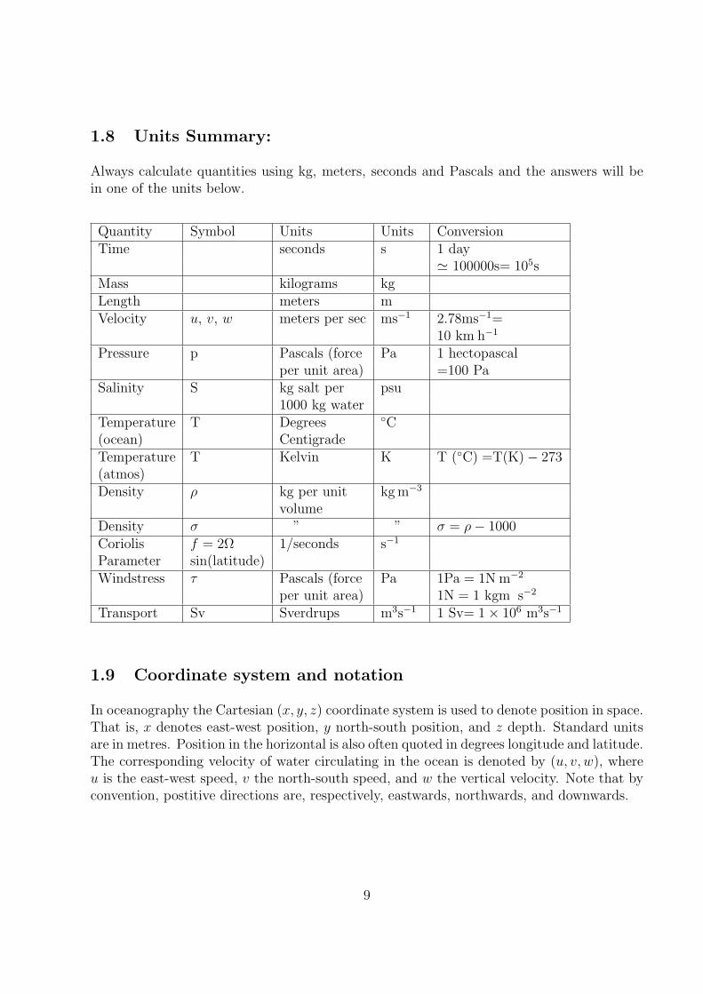
1.8 Units Summary:

Always calculate quantities using kg, meters, seconds and Pascals and the answers will bein one of the units below.

Quantity Symbol Units Units ConversionTime seconds s 1 day

' 100000s= 105sMass kilograms kgLength meters mVelocity u, v, w meters per sec ms−1 2.78ms−1=

10 km h−1

Pressure p Pascals (force Pa 1 hectopascalper unit area) =100 Pa

Salinity S kg salt per psu1000 kg water

Temperature T Degrees C(ocean) CentigradeTemperature T Kelvin K T (C) =T(K)− 273(atmos)Density ρ kg per unit kg m−3

volumeDensity σ ” ” σ = ρ− 1000Coriolis f = 2Ω 1/seconds s−1

Parameter sin(latitude)Windstress τ Pascals (force Pa 1Pa = 1N m−2

per unit area) 1N = 1 kgm s−2

Transport Sv Sverdrups m3s−1 1 Sv= 1× 106 m3s−1

1.9 Coordinate system and notation

In oceanography the Cartesian (x, y, z) coordinate system is used to denote position in space.That is, x denotes east-west position, y north-south position, and z depth. Standard unitsare in metres. Position in the horizontal is also often quoted in degrees longitude and latitude.The corresponding velocity of water circulating in the ocean is denoted by (u, v, w), whereu is the east-west speed, v the north-south speed, and w the vertical velocity. Note that byconvention, postitive directions are, respectively, eastwards, northwards, and downwards.

9

1.10 Gradients and derivatives

In most applications in oceanography the gradient terms in equations, such as

dT

dx,

dρ

dtetc.

can be approximated as follows:dT

dx' ∆T

∆x

where ∆ means the ‘change in’ a certain property (temperature, time, and so on). This isgenerally valid for ‘small’ ∆x.

10

2 The Equations of Motion

To understand the circulation of the oceans and atmosphere it is necessary to examine theunderlying equations which govern their motion. In the following, the equations are all de-rived from a consideration of Newton’s law F = ma where F denotes the applied force ona fluid parcel of mass m and a the resultant acceleration. Fluid mechanics in oceanographyis based on newtonian mechanics where we consider conservation of Mass (continuity equa-tion), Conservation of Energy (conservation of heat, heat budgets, mechanical energy, andwave equations) Conservation of Momentum (Navier Stokes Equations) and Conservation ofAngular Momentum (conservation of vorticity).

We will use the primitive equations, which are a version of the Navier-Stokes equationsthat describe hydrodynamic flow on the sphere (the earth) under the assumptions thatvertical motion is much smaller than horizontal motion (hydrostatic approximation) andthat the fluid layer depth is small compared to the radius of the sphere. Thus, they are agood approximation of global ocean and atmospheric flow and are used in most ocean andatmospheric models. In general, nearly all forms of the primitive equations relate the fivevariables u =(u,v,w), T, p and their evolution over space and time.

2.1 The Vertical Equation

In the vertical direction, the two most important forces are those that result from gravityand changes in pressure. Consider a small cylinder of fluid of mass m as shown in Figure 2.1.

The force downwards due to gravity g is mg. The mass of the cylinder also leads to anincrease in pressure (force/unit area) from z1 to z2 = z1 + ∆h. This increase in pressureleads to a net force upwards given by

[p(z1)− p(z2)

∆h

]V ' −dp

dzV (2.1)

where V is the volume of the cylinder. Now since m = ρV , the acceleration of the cylindera = dw/dt is equal to the sum of all the forces F/m so that

dw

dt= −1

ρ

dp

dz+ g (2.2)

In the absence of vertical motion w = 0 and (2.2) reduces to

dp

dz= ρg (2.3)

the Hydrostatic Balance, where the gradient of pressure supports the fluid against theforce of gravity. Even in the presence of vertical motion the hydrostatic balance is a verygood model for long period motions.

11

z1 p1 -m.dp/ dz

z2 p2 mgm

Figure 2.1: The Hydrostatic Balance

Example:To show this assume that w ∼ W = 0.01ms−1 and that the period of motions is T ∼ 1 day(8.64× 104 seconds). W and T represent typical values. In this case we scale

dw

dt∼ W

T∼ 0.01

105∼ 10−7m s−2 (2.4)

This term may be compared with g = 9.8m s−2 and is thus very small. Gravity cannot be

balanced by dw/dt and must be balanced by−1

ρ

dp

dzso that (2.3) is a very good approximation

for motions of period a day or more.

To proceed we shall partition the density into two components, ρ = ρ0 + σT , where ρ0 =1000 kg m−3 and as shown in the Figure 2.2, σT ∼ 20− 30 kg m−3. Now we shall also definetwo components of pressure each of which is to balance ρ0 and σT . We define p0 by

dp0

dz= ρ0g (2.5)

and p′ bydp′

dz= σT g (2.6)

so that p = p0 + p′. The pressure p0 is from (2.5) given by

p0 = ρ0gz (2.7)

12

and is called the static pressure. It is only related to the constant density ρ0 = 1000 kg m−3

and serves to support the bulk of the water mass between z = 0 and the depth z (Figure 2.2).The component p′ is of more interest since it is related to η and σT and thus to variations

z=0

z po= ogz

p'= og

p=po+p'

Figure 2.2: Perturbations in Sealevel

in sea level and variations in the distribution of heat (and salt) and, ultimately, to thecirculation of the oceans and atmosphere. Since σT will be a function of z we cannotin general simplify (2.6) further but note that the density field σT is also in hydrostaticequilibrium.

A major simplification can be made if we can assume that σT is zero and the density of theocean is everywhere constant so that ρ = ρ0. In this case (2.6) reduces to

dp′

dz= 0 (2.8)

and since p0 supports the mass from to the surface to a depth z, p′ supports the residualmass from z = 0 the surface to z = η (see the figure) i.e.

p′ = ρ0gη (2.9)

Note that while η may vary with x, y and t it is independent of depth (as is p′). An ocean oratmosphere in which density is constant is called barotropic and for ocean shelves, where the

13

water is well mixed, (Equation 2.9) is a very good approximation. Indeed, measurementsof bottom pressure in the ocean (depth h) can be used to obtain p′ from p′ = p − ρ0ghand thus sea level variations η. Finally, it is worth noting that by measuring pressure onan instrument that the depth z of the instrument may be very accurately obtained. SinceσT ¿ ρ0 we have p0 À p′ so that p ' p0 = ρ0gz.

2.1.1 Equations of State

Oceans: For the oceans, the density ρ depends on the temperature T (C), the salinity Sand on the pressure p and can be approximated by a relation known as the equation of state,

ρ = ρ00(1− αT + βS), (2.10a)

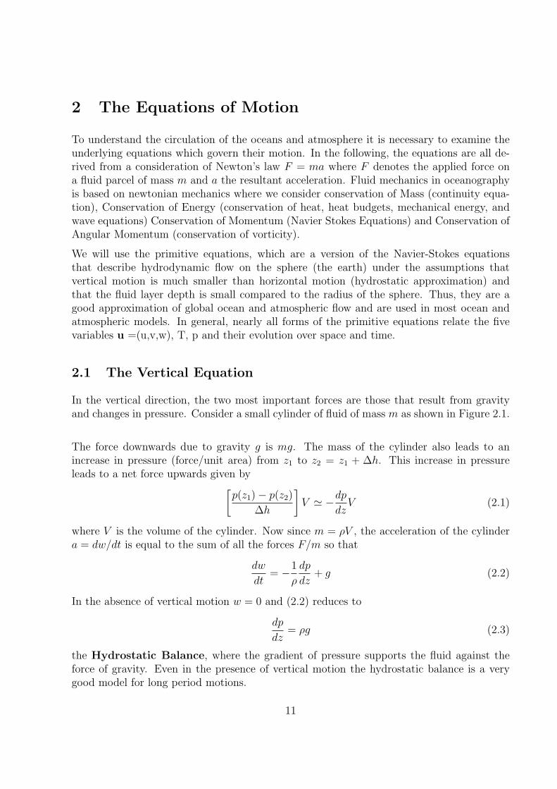
where α and β depend on temperature, salinity and pressure and ρ00 is some constant density.Note that in the relation above, larger temperatures mean the water is less dense while largervalues of salinity mean the water is denser.

Figure 2.3: Typical values of Temperature, Salinity and Density.

Atmosphere: For the atmosphere, the density may be written in terms of the temperatureT (expressed in Kelvin; 273 K = 0C) and to a good approximation, the equation of state isgiven by

ρ =p

RT(2.10b)

where R = 287J/(kg K) and T is given in K. Figure 2.4 shows a mean vertical profileof temperature in the atmosphere, with increasing height above the Earth’s surface. TheLapse Rate is the rate at which temperature decreases with height in the atmosphere. Thishas the opposite sign from the temperature gradient a physicist would use, so be careful.Throughout the bottom 10 − 15 km of the atmosphere the lapse rate is ∼ 6.5 K/km. Thisis a typical value, where daytime convection stirs things up.

14

Figure 2.4: Vertical Profile of Temperature (K) in the Atmosphere

Over the first 10 km or so is the troposphere which contains 80% of the atmosphere’s massand nearly all the water vapour. It is characterised by vertical mixing, storms and latentheat release. Jets typically fly above this layer so as to avoid the “weather”.

Above this layer lies the stratosphere which is poorly mixed. The temperature increaseswith height due to the radiative balances with the sun (discussed later).

From the above, the hydrostatic balance for the atmosphere may be written as

dp

dz=

gρ

RT

and from the figure above we take T to be approximately constant and equal to 250 K. Inthis case we may integrate the above from z = 0 to some height to obtain

p = pa exp(z/Hc)

where pa is some surface pressure and Hc = RT/g is an e-folding scale height equal to about7 km. That is, over this height the pressure drops by 1/e = 1/2.78 or about a third. (Recallthat we take z to be negative upwards.)

2.2 Buoyancy Effects

Gravity acts on vertical density gradients in the ocean or atmosphere to either stabiliseor destabilise the column of fluid. Here we shall quantify how vertical changes in density

15

can act to stabilise vertical movement of water parcels. Consider an ocean with densitydependent only on depth: ρ = ρ(z), with z zero at the surface and increasing with depth.For convenience, let us assume that ρ increases linearly with depth according to:

ρ(z) = ρ0 + kz = ρ0 + zdρ

dz(2.10c)

where k = dρ/dz is a constant. Now if a parcel is moved from z = z1 to a depth z = z2 i.eit displaces more dense fluid as shown in Figure 2.5.

o (z)

z

z =0

z

Figure 2.5: Oscillation of a parcel of fluid in the ocean.

Archimedes tells us that the force on the parcel will be equal to the mass displaced timesgravity g (9.8 m s−2) i.e. the acceleration a is

a = g(ρ0 − ρ(z))/ρ0 (2.10d).

If dρ/dz > 0 then ρ(z) > ρ0 so that density at depth is larger than at the surface. Inthis case a < 0 and the acceleration (force/unit mass) is upward. Thus, the tendency isfor the parcel to be forced back to its initial position. The negative force acts to push theparcel back to where it came from. It is this restoring force that inhibits mixing in both theatmosphere and the ocean, (hence keeping cold water at depth in the ocean). In addition,the restoring force prevents the ready mixing of greenhouse gases into the ocean. Assuminga linear density gradient (as in Figure 2.5), a movement from z = 0 to z will result in adensity difference given by

ρ′ = (dρ

dz)(z − zo)

and the acceleration isdw

dt=−g

ρ0

dρ

dz(z − zo)

16

Now with z the position of the parcel, the acceleration is a = d2z/dt2 (t is time) and puttingρ(z) we get

d2z

dt2= a = −z

(g

ρ0

dρ

dz

)

Let us define

N2 =g

ρ0

dρ

dz(2.10e)

(we will see why below), so thatd2z

dt2= −N2z

This is a differential equation for the motion of the fluid parcel. A solution is

z = A sin(Nt)

where the amplitude A is unknown. However, we do know that the parcel will move like aspring with frequency N , the buoyancy or Brunt-Vaisala frequency.

The period T is given byT = 2π/N

so that if dρ/dz is large (i.e., the stratification strong), then N is large and T small i.e. fastoscillations in a strongly stratified ocean. If dρ/dz is small (e.g., in the deep ocean), however,then N is small and T is large. Such waves in the atmosphere can be seen as parallel linesof clouds.

2.3 The Horizontal Equations

In the horizontal (x, y) plane pressure gradients will also result in forces on fluid parcels.In the following we will consider a barotropic ocean so that these forces may be thought toact over the entire column depth. The forces due to horizontal pressure gradients may bewritten as

− 1

ρ0

dp′

dxand − 1

ρ0

dp′

dy(2.11)

and we note that only p′ appears since the static pressure p0 is only a function of z.

2.3.1 The Coriolis Force

The second force that must be considered is that which arises from the rotation of the Earth.To illustrate this force consider the rotating table as sketched below with two observers B,at rest and A, spinning with the table. Now if A rolls a ball towards B, the observer B willsee the ball move in the strait line indicated. Observer A however will say that the ball wasdeflected to the left. The ‘force’ which does this only appears to the observer in the rotatingreference frame and only acts on moving objects.

17

B

fv

v A

A

.

Figure 2.6: The Coriolis Force

If Ω denotes the angular speed of the turntable (radians/sec) then the force is given by2ΩUm where U and m are the velocity and mass of the ball. For the Earth, the localangular speed varies with latitude. At the equator it is zero, while at the poles it is largest(2π/8 · 64× 104 sec). A convenient way of expressing this is through the Coriolis parameter

f = 2Ω sin(latitude)

and the acceleration due to the Coriolis force is given by

fv and − fu (2.12)

in the x and y directions respectively. Note v and u are the velocities in the y and xdirections. In the northern hemisphere the Coriolis force acts to deflect to the right and fis positive. In the southern hemisphere the reverse holds.

Now collecting the forces we have the following horizontal equations (a = F/m)

du

dt= − 1

ρ0

dp′

dx+ fv (2.13a)

dv

dt= − 1

ρ0

dp′

dy− fu (2.14a)

and in the vertical (2.6):

0 = −dp′

dz+ σT g

For a barotropic ocean where σT = 0 and p′ = ρ0gη the above simplify to

du

dt= −g

dη

dx+ fv (2.13b)

dv

dt= −g

dη

dy− fu (2.14b)

18

2.4 The Geostrophic Balance

The above equations may be simplified further for motions with periods of 10 days or more.To see this we again perform a scaling analysis on (2.13) and (2.14) and choose a periodT ' 10 days = 8 · 64× 105 seconds. (Always work in mks - meters, kilograms and seconds).With f ' 10−4 sec−1 (latitude ' 40) and assuming that u ' v ' U , an unknown scalevelocity, then

du

dt∼ dv

dt∼ U

T∼ U × 10−6 sec−1,

while fv ∼ fu ∼ fU ∼ U × 10−4 sec−1 .Thus, the acceleration terms are a hundred times smaller than the Coriolis terms and negli-gible for these long period motions. In this case the equations (2.13)–(2.14) reduce to

0 = − 1

ρ0

dp′

dx+ fv (2.15a)

0 = − 1

ρ0

dp′

dy− fu (2.15b)

which is known as the geostrophic balance. The deflection by the Coriolis force is now bal-anced by the force due to the gradients of pressure. As an example consider the atmosphericHigh–Low system sketched in Figure 2.7. The fluid parcel shown does not rush from Highto Low (the pressure gradient force) but instead is balanced by a Coriolis force associatedwith motion in the y direction.

SH Plan View

v

CF PG

LH

x

Figure 2.7: Geostrophic Balance in the Southern Hemisphere CF=fv and PGF=dp

ρdx

19

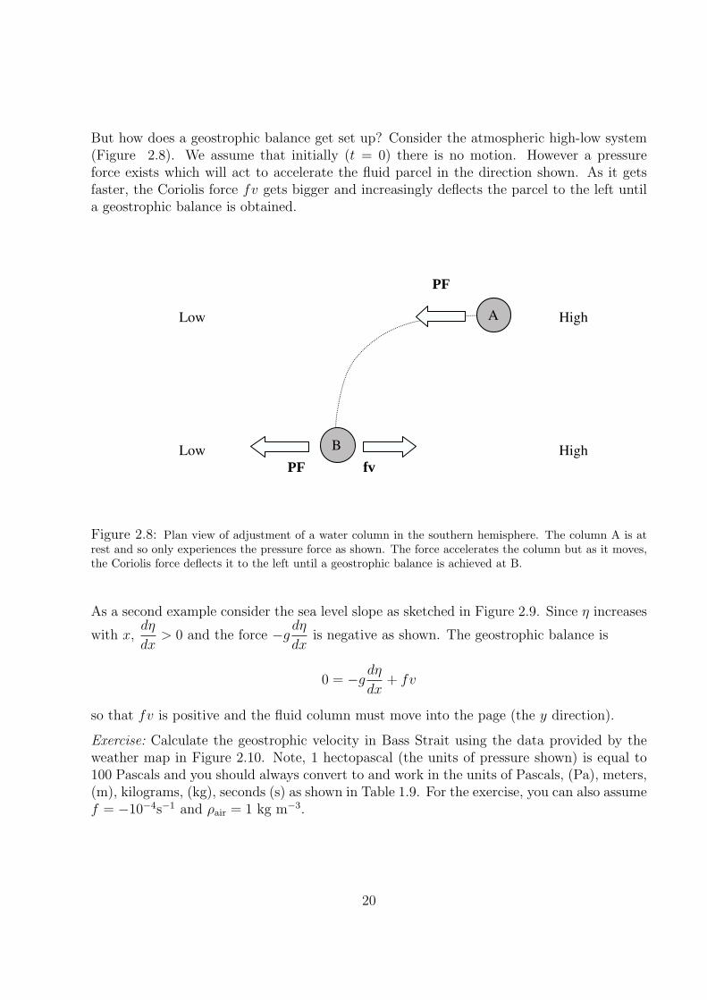
But how does a geostrophic balance get set up? Consider the atmospheric high-low system(Figure 2.8). We assume that initially (t = 0) there is no motion. However a pressureforce exists which will act to accelerate the fluid parcel in the direction shown. As it getsfaster, the Coriolis force fv gets bigger and increasingly deflects the parcel to the left untila geostrophic balance is obtained.

PF

Low High

Low High PF fv

B

A

Figure 2.8: Plan view of adjustment of a water column in the southern hemisphere. The column A is atrest and so only experiences the pressure force as shown. The force accelerates the column but as it moves,the Coriolis force deflects it to the left until a geostrophic balance is achieved at B.

As a second example consider the sea level slope as sketched in Figure 2.9. Since η increases

with x,dη

dx> 0 and the force −g

dη

dxis negative as shown. The geostrophic balance is

0 = −gdη

dx+ fv

so that fv is positive and the fluid column must move into the page (the y direction).

Exercise: Calculate the geostrophic velocity in Bass Strait using the data provided by theweather map in Figure 2.10. Note, 1 hectopascal (the units of pressure shown) is equal to100 Pascals and you should always convert to and work in the units of Pascals, (Pa), meters,(m), kilograms, (kg), seconds (s) as shown in Table 1.9. For the exercise, you can also assumef = −10−4s−1 and ρair = 1 kg m−3.

20

z=0 v

-gd /dx fv

x

Figure 2.9: Sealevel Slope and Geostrophy

Figure 2.10: Surface Atmospheric Pressure in hectopascals (MSLP).

2.5 The Thermal Wind Balance

In the above we have assumed that density ρ is constant. However, small horizontal changesin density can result in large vertical changes in current, particularly near fronts and eddies.

For a Geostropic balance we have from (2.15)

21

v =1

ρf

dp

dx(2.16a)

u = − 1

ρf

dp

dy(2.16b)

and the hydrostatic balancedp

dz= ρg

Now differentiating (2.16a) and (2.16b) with respect to z (depth) we get

dv

dz=

1

ρ0f

d

dz

(dp

dx

)=

1

ρ0f

d

dx

(dp

dz

)(2.17a)

du

dz=

1

p0f

d

dy

(dp

dz

)(2.17b)

where since ρ is very nearly constant, the density in the denominator of (2.7) is taken as theconstant ρ0.

Now substituting for dp/dz we get

dv

dz=

g

ρ0f

dρ

dx(2.18a)

du

dz= − g

ρ0f

dρ

dy(2.18b)

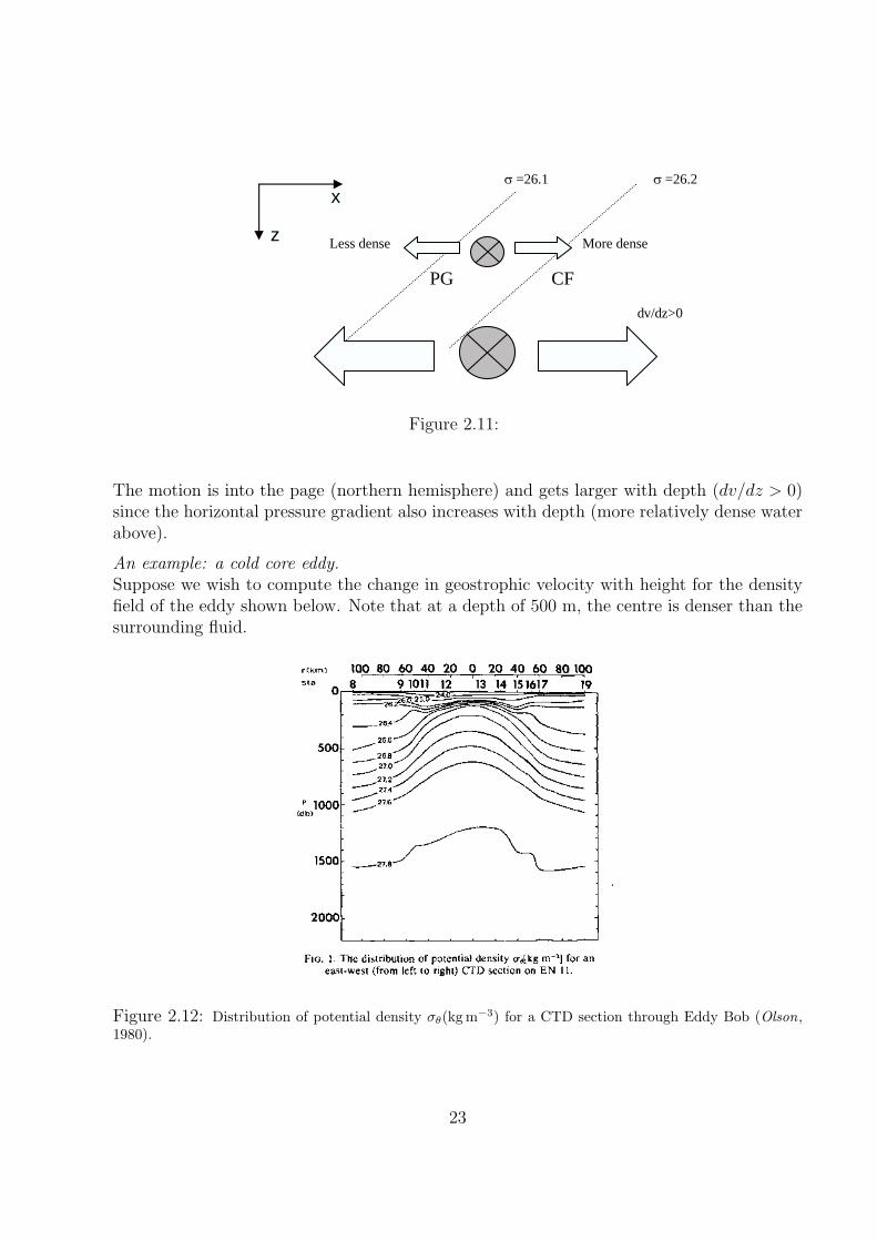
the ‘thermal wind’ balance. The balance (2.18) may again be thought of in terms of forces.Consider the sloping density surfaces shown below. Due to the weight of the water, therelatively denser water on the right leads to a pressure force (PF) as shown and this isbalanced by a Coriolis force.

22

=26.1 =26.2

Less dense More dense

PG CF

dv/dz>0

x

z

Figure 2.11:

The motion is into the page (northern hemisphere) and gets larger with depth (dv/dz > 0)since the horizontal pressure gradient also increases with depth (more relatively dense waterabove).

An example: a cold core eddy.Suppose we wish to compute the change in geostrophic velocity with height for the densityfield of the eddy shown below. Note that at a depth of 500 m, the centre is denser than thesurrounding fluid.

Figure 2.12: Distribution of potential density σθ(kg m−3) for a CTD section through Eddy Bob (Olson,1980).

23

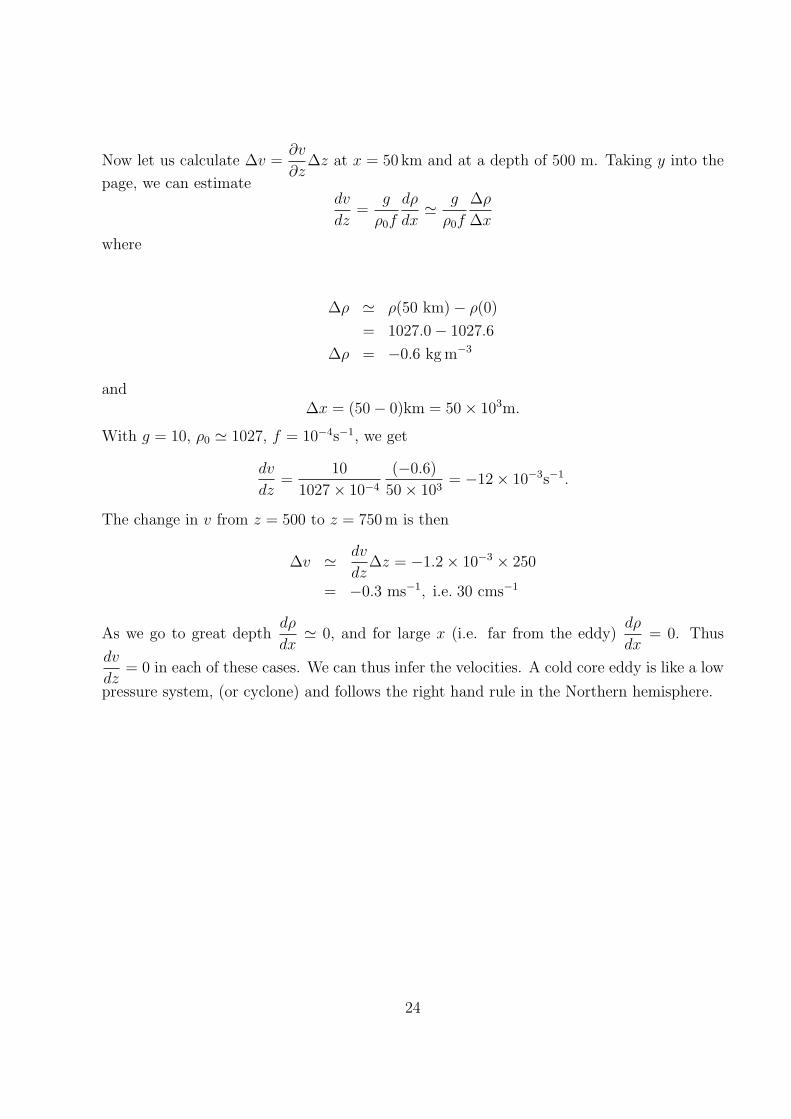
Now let us calculate ∆v =∂v

∂z∆z at x = 50 km and at a depth of 500 m. Taking y into the

page, we can estimatedv

dz=

g

ρ0f

dρ

dx' g

ρ0f

∆ρ

∆x

where

∆ρ ' ρ(50 km)− ρ(0)

= 1027.0− 1027.6

∆ρ = −0.6 kg m−3

and∆x = (50− 0)km = 50× 103m.

With g = 10, ρ0 ' 1027, f = 10−4s−1, we get

dv

dz=

10

1027× 10−4

(−0.6)

50× 103= −12× 10−3s−1.

The change in v from z = 500 to z = 750 m is then

∆v ' dv

dz∆z = −1.2× 10−3 × 250

= −0.3 ms−1, i.e. 30 cms−1

As we go to great depthdρ

dx' 0, and for large x (i.e. far from the eddy)

dρ

dx= 0. Thus

dv

dz= 0 in each of these cases. We can thus infer the velocities. A cold core eddy is like a low

pressure system, (or cyclone) and follows the right hand rule in the Northern hemisphere.

24

ww

w.annualreview

s.org/aronlineA

nnual Review

s

Annu. Rev. Earth Planet. Sci. 1991.19:283-311. Downloaded from arjournals.annualreviews.orgby UNIVERSITY OF NEW SOUTH WALES on 03/06/07. For personal use only.

Figure 2.13: Velocity and Stratification through a cold core eddy (left) and a warm-core eddy (right)(Olson, 1991).

2.5.1 An Example: an atmospheric front

For the atmosphere we have

f∂v

∂z=

g

ρ

∂ρ

∂x, f

∂u

∂z=−g

ρ

∂ρ

∂y

and ρ = p/RT . It turns out that changes of p with x and y can be neglected compared tochanges in T so that the above become

f∂v

∂z=−g

T

∂T

∂x, f

∂u

∂z=−g

T

∂T

∂y. (2.19)

Now consider a cold front that is being advected at a speed U0 towards us (Figure 2.14):

In region (1) the hot air is well mixed and∂T

∂x= 0 so that v is zero or constant. In region

(2), the front exists and since∂T

∂xis positive, f

∂v

∂zis negative. In the southern hemisphere f

is negative and so∂v

∂zis positive and v increases from zero (above the front) to some positive

25

Uo

z Cold Air (3) (2) (1) Hot Air

x

Figure 2.14: An example of a cold front in the atmosphere

value below the front. That is the temperature suddenly drops and the wind veers abruptlyto the right if we are facing the front.

How big is the wind? Suppose T changes by ∆T = 10C over ∆x = 100 km then∂T

∂x∼

∆T

∆x∼ 10−4 Km−1. With g = 10 m s−2, f = −10−4s−1 and T ' 300K we get

∂v

∂z=−g

fT

∂T

∂x' 0.03s−1.

The change ∆v over some height ∆z is then

∆v ' ∂v

∂z∆z

and if we take ∆z to be 2000 m we get ∆v ' 60 ms−1 or 200km/hr!

2.6 Taylor Sheets, Columns and Blocking

The thermal wind relations are

f∂v

∂z=

g

ρ0

∂ρ

∂x

f∂u

∂z=

−g

ρ0

∂ρ

∂y

so that if the ocean/atmosphere is homogeneous (well mixed) and ρ = ρ0 a constant then

∂v

∂z=

∂u

∂z= 0, (2.20)

26

and the horizontal velocities (u, v) do not vary with height or depth. This ‘vertical rigidity’is a fundamental property of a rotating homogeneous fluid.

The nature of the vertical velocity can also be determined. Since the motion is also geostropicwe have

∂u

∂x=

∂

∂x

(1

ρ0f

∂p

∂y

)= −∂v

∂y= − ∂

∂y

(−1

ρ0f

∂p

∂x

)

so that ux + vy = 0. Now it can be shown that the velocity field also satisfies the condition

ux + vy + wz = 0.

In this case, if ux + vy = 0 then we must have

∂w

∂z= 0 (2.21)

as a corollary of (2.20) above, and w also is independent of z.

2.6.1 Experiment: Taylor Curtains

1.4. SCALES OF MOTIONS

Figure 2.15: Taylor Curtains (Cushman-Roisin and Beckers, 2007)

2.6.2 Taylor Columns:

An oceanographic example of a Taylor Column is the example of flow post a seamount(Figure 2.16). Since (u, v, w) cannot vary with z, the flow is around the seamount whileabove it there is no motion: Implications for marine ecology.

27

No motion

Side View Plan View

Figure 2.16: Flow past a Seamount

2.6.3 Blocking

The onshore sea breeze below will be blocked by the presence of the mountain range just asin the case of the Taylor column: Implications for pollution in Sydney’s west.

Stagnant region

Sea Breeze

Ocean

Figure 2.17: Blocking of the onshore seabreeze in Sydney’s west.

28

2.7 The effects of Friction

The presence of turbulence acts to increase the frictional drag of the oceans and atmosphere,notably near coastal boundaries and the air-sea interface. For motions of period 3 days orlonger a simple model for the frictional force due to the sea floor (or land) is given by

−ru/h and − rv/h

in the x and y directions where h is the ocean depth and r a coefficient given by

r = CDv∗.

CD ' 2 × 10−3 is a non–dimensional drag coefficient and v∗ denotes a typical turbulent ortidal velocity. The equations of motion (2.13) and (2.14) then become

du

dt= −g

dη

dx+ fv − ru/h (2.22)

dv

dt= −g

dη

dy− fu− rv/h. (2.23)

The effects of friction are readily seen if we consider the simpler balance

du

dt= −ru/h.

A solution isu = u0e

−rt/h

so that at t = 0 u = u0 while as t becomes large, u becomes small. Clearly (h/r) plays therole of an e–folding time scale of frictional spin down. For r = 5×10−5m sec−1 and h = 70m(Bass Strait) h/r = 16 · 2 days. Friction thus acts to damp out motion.

2.8 Conservation of Mass and Compressibility in the Ocean andAtmosphere

Conservation of mass is an important constraint on fluid motion. If we consider a fixed fluidvolume, the mass of the fluid occupying the volume may change with time if the densitychanges, however mass continuity tells us that this can only occur if there is flux of massinto or out of the volume.

du

dx+

dv

dy+

dw

dz= 0 (2.24)

The definition of incompressible flow is that it is non-divergent, however for any real fluid,it is never exactly obeyed. For incompressible flow such as liquid in the ocean we can

29

consider a simplified approximation to the continuity equation. For the barotropic oceanwith variations in sea levell it may be written as:

dη

dt+

d(hu)

dx+

d(hv)

dy= 0 (2.25)

and expresses the fact that as sea level changes, water must flow in or out in compensation(Figure 2.18). For v = 0 and h =constant (2.22) becomes

dη

dt+ h

du

dx= 0.

up down up

x

h

u u

Figure 2.18: Continuity

In comparison, a compressible fluid such as air is nowhere close to being non-divergent, thisis because the density changes drastically as the fluid parcels expand and contract. Thisis very inconvenient in the analysis of atmospheric dynamics. A simplification exists if thehydrostatic approximation is valid, and if we adopt pressure co-ordinates. In the pressurecoorindate version of the continuity equation there is no term representing the rate of changeof density it is simply:

du

dx+

dv

dy+

dw

dp= 0 (2.26)

The simplicity of this equation is one reason why pressure coordinates are favoured in me-teorology.

30

3 Unforced Motions: Waves

The goal of this chapter is two fold, 1. to introduce the concepts of waves, and some simpleaspects of wave theory, and 2. to relate this to examples in the ocean and the atmosphere.We will consider unforced motions that satisfy the equations of motion (2.13)–(2.14) and(2.22). We will begin with surface gravity waves where the effects of the Earth’s rotation areunimportant and then consider waves for which this is not the case. This will lead to theconcept of the potential vorticity (or spin) of a fluid column which is vital in understandinglarge scale ocean circulation.

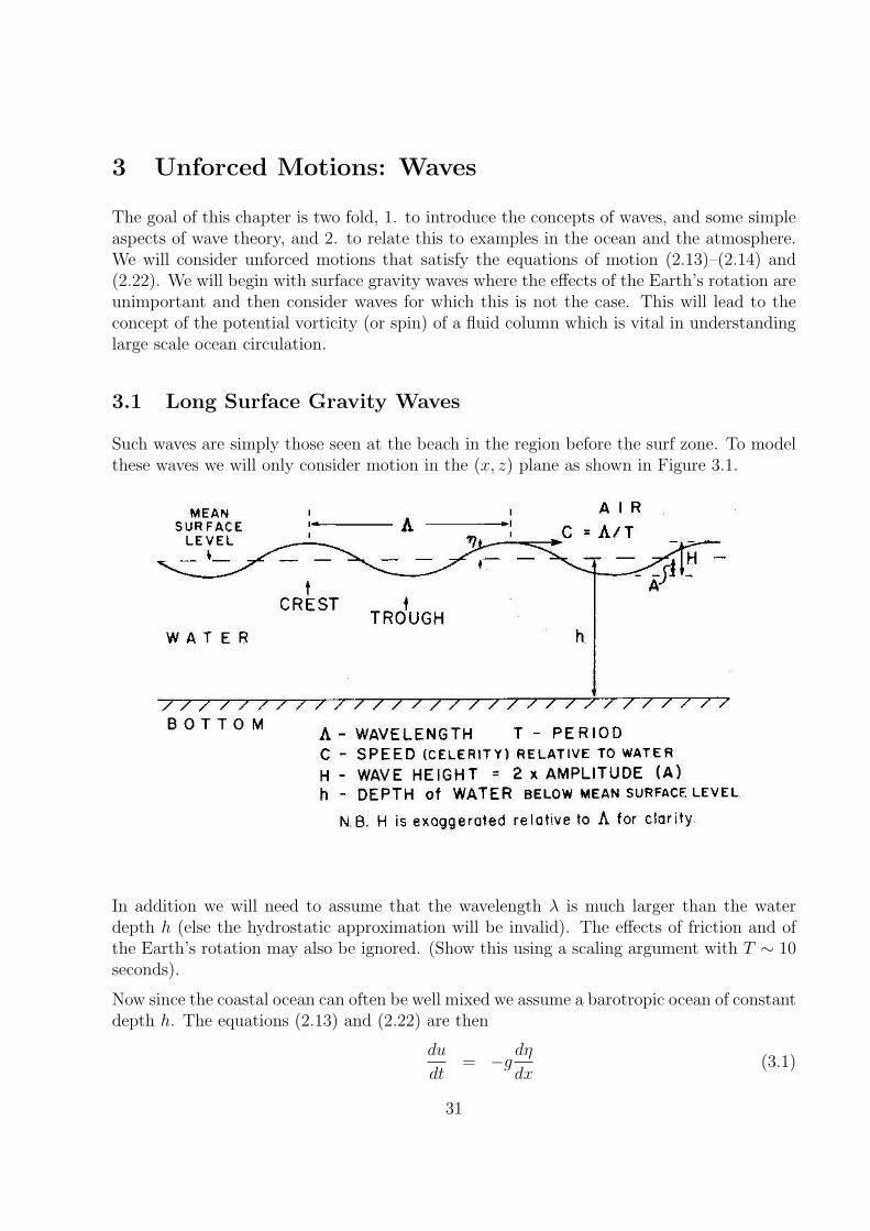
3.1 Long Surface Gravity Waves

Such waves are simply those seen at the beach in the region before the surf zone. To modelthese waves we will only consider motion in the (x, z) plane as shown in Figure 3.1.

In addition we will need to assume that the wavelength λ is much larger than the waterdepth h (else the hydrostatic approximation will be invalid). The effects of friction and ofthe Earth’s rotation may also be ignored. (Show this using a scaling argument with T ∼ 10seconds).

Now since the coastal ocean can often be well mixed we assume a barotropic ocean of constantdepth h. The equations (2.13) and (2.22) are then

du

dt= −g

dη

dx(3.1)

31

dη

dt+ h

du

dx= 0 (3.2)

and by differentiating Eq 3.1 with respect to x and Eq 3.2 with respect to t we obtain thewave equation.

d2η

dt2− gh

d2η

dx2= 0 (3.3)

Let us consider a plane wave solution of the form

η = A cos(kx− ωt) (3.4)

where ω = 2π/T is the frequency and k = 2π/λ is the wavenumber.

The wave period T is the time it takes two successive wave crests or troughs to pass a fixedpoint. The wave length, λ is the distance between two successive waves crests or troughs ata fixed time. The wave number, k represents the number of crests in the x direction.

Frequency and period are distinctly different, yet related, quantities. Frequency refers to howoften something happens; period refers to the time it takes something to happen. Frequencyis a rate quantity; period is a time quantity. Frequency is the cycles/second; period is theseconds/cycle.

3.1.1 Dispersion relation

Wave frequency ω is related to wave number k by the dispersion relation

ω2 = g k tanh(kh)

Approximations can be made in both shallow and deep water. These will be discussedfurther in Section 3.3. Here we will investigate the shallow water wave approximation,which is valid if the water depth is much less than a wavelength. In this case h << λ,kh << 1 and tanh(kh) = kh.

Substituting Eq 3.4 into Eq 3.3 we get

−ω2A cos(kx− ωt) + hgk2A cos(kx− ωt) = 0

Cancelling the term A cos(kx− ωt) results in the shallow water dispersion relation:

ω2/k2 = hg

orc = ω/k =

√gh (3.5)

The quantity c ≡ ω/k is called the phase speed and is the rate at which wave crests (ortroughs) pass a fixed point. This may be seen from Eq 3.4 where for η = A (a crest) wemust have kx− ωt = 0 (say) so that we must change x by the amount

x =ω

kt

to keep up with the crest (Figure 3.1).

32

x=ct

c=ω/k

Figure 3.1: Displacement of the crest of a wave

Now returning to Eq 3.5, the wave is only a solution if c =√

gh, so that if h = 2 m thenc = 4.4 ms−1. Given we know the wave period, e.g T = 3 sec, then since c = ω/k = λ/T wehave λ = cT so that λ = 13.3 m.

3.2 Wave Refraction, Diffraction and Shoaling

3.2.1 Refraction

If you look out from any headland you will see that wave crests tend to become parallel tothe shore as the wave moves inshore.

I J150m

CI

CJ

I

J

Coast

100 m

50 m

20 m

Figure 3.2: Wave refraction as it approaches shallow water.

33

Exercise: A wave has a frequency ω = 2π/4s−1 in 100 m of water. Calculate c and λ.Calculate c and λ after the wave has reached a depth of 10 m of water. Explain what hashappened.

Now consider two parts I and J of a wave crest. Offshore, the crests move at a speedcI = cJ =

√gh ' √

10× 50 ms−1. As the wave moves further in, the crest J is in deeperwater so that

cJ =√

ghJ > cI =√

ghI

since hJ > hI . Thus, the wave crest at J moves faster and the wave tends to become moreparallel with the shoreline.

3.2.2 Shoaling

Shoaling is the term for the changes in wave characteristics that occur when a wave reachesshallow water. As well as slowing, waves steepen as the depth decreases. This observationmay be explained using the following formulae for the flux of energy Γ:

Γ = cE (3.6)

where c is the wave phase speed and

E =1

2ρ0gA2 (3.7)

is the total kinetic and potential energy of the wave (due to motion and sea–level variations)for

η = A cos(kx− ωt).

Now consider a profile of the beach shown in Figure 3.3. In the absence of friction and wavebreaking the energy flux at I is equal to that at J so that

ΓI = cIEI = ΓJ = cJEJ (3.8)

andEJ = (cI/cJ)EI (3.9)

From Eq 3.7 we then haveA2

J = (hI/hJ)12 A2

I

so that with hJ < hI , the amplitude of the wave AJ is larger than AI , i.e. the wave steepens.

In summary the decreasing depth causes: (a) An increase in wave height - The conservationof energy results in more energy forced into a smaller area. Since wave energy is proportionalto wave height squared, this increases wave height as it propagates toward shore even thoughsome of the energy is dissipated by bottom friction.

34

Flux

i j

Ci Cj

Figure 3.3: Steepening / Shoaling of a wave as it approaches the shore.

(b) A decrease in wave speed - Remember that waves in shallow water have speeds that aredependent on the square root of water depth. As the depth decreases, so too will the wavespeed.

Refraction is the change in direction of a wave due to a change in its speed. This is mostcommonly seen when a wave passes from one medium to another, or in the case of the ocean,moves from deep water into shallow water. Refraction of ocean waves generally occurs asthey approach the shore. This process unevenly distributes wave energy along the shoreline,and results in erosion at headlands and deposition on beaches.

Diffraction refers to the various phenomena associated with wave propagation, such as thebending, spreading and the interference of waves passing by an object. In the ocean wavediffraction results from wave energy being transferred around or away from barriers impedingits forward motion. e.g. waves move past barriers into harbours because their energy moveslaterally along the crest of the wave, and the wave behind the barrier goes out in all directions(Thurman and Burton, 2001)

3.2.3 Wave Breaking

As the wave moves into shallower water, shoaling affects the wave form by slowing its basewhile having less effect on the crest. At some point, the crest of the wave is moving too fastfor the bottom of the wave form to keep up. The wave then becomes unstable and breaks.For a wave of the form

η = A cos(kx− ωt)

35

observations show that steepening will occur and the wave will break if the amplitude getssufficiently large and

A & λ/12.

Alternatively, if the water gets too shallow, the wave will break if

A & 0.8h.

In meteorology, gravity waves are said to break when the wave produces regions where thepotential temperature decreases with height, leading to energy dissipation through convectiveinstability; likewise Rossby waves are said to break when the potential vorticity gradient isoverturned.

3.3 Shallow and Deep Water Waves

The waves described above are restricted to the case where λ À h, or kh ¿ 1. Moregenerally, it can be shown that

c =ω

k=

[g

ktanh(kh)

] 12

(3.10)

and if λ À h(kh ¿ 1) this reduces to shallow water waves above where c =ω

k=

√gh.

Where λ < 2h we have deep water waves and Eq 3.10 becomes

c =ω

k= (g/k)

12 = (gλ/2π)

12

36

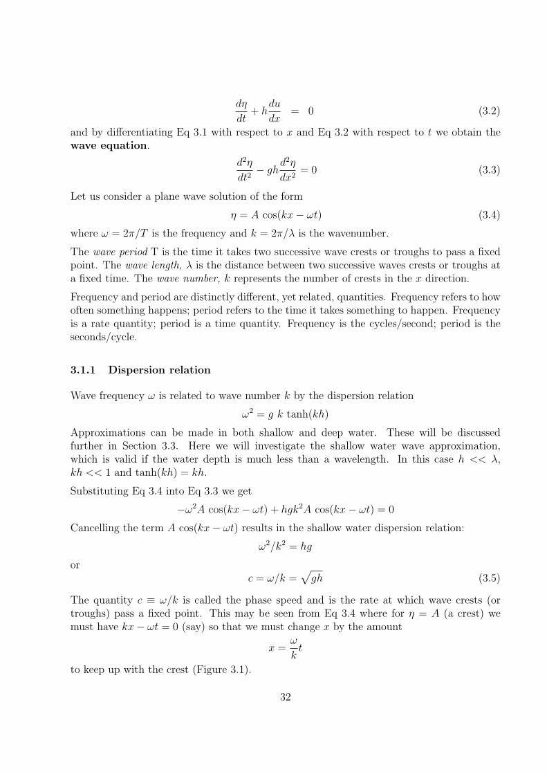
3.4 Resonance

Tides are long gravity waves driven by the gravitational attraction of the moon, sun andEarth. The amplitude of the tide may be greatly enhanced by resonance with bays ofparticular sizes. Consider a bay of length L:

z=hx

L

Tide

Now suppose the tides drive a sea level signal at x = L given by

ηTide = η0 cos ωt,

where ω = 2π/(tidal period) and η0 is constant. Now to illustrate resonance, assume asolution to Eq 3.3, the wave equation,

η = A cos kx cos ωt, (3.11)

where again c =ω

k=

√gh. At x = 0, ut = −gηx = 0 since u = 0. Equation 3.11

satisfies this, since ηx ∝ sin kx = 0. Equation 3.11 is also a solution to the wave equation if

c =ω

k=

√gh.

At x = L, we match sea-level of the solution to ηTide

η = A cos kL cos ωt = η0 cos ωt

so that A is given byA = η0/ cos kL.

Now cos kL will be zero if kL =π

2(+ 2nπ). With c =

ω

k, k =

ω

cthe condition kL =

π

2will

be met if

L =π

2k=

πc

2ω=

cT

4

37

If the length of the bay is such that

L =cT

4=

T

4

√gh

then cos kL ' 0 and A = ηcos(kL)

becomes infinite. In practice, frictional effects due to bottominteraction prevent the resonance going to infinity. This is called a quarter wave resonatorand sea level is as shown in Figure 3.4.

ATide

Lx

z=h

Examples: Bay, of Fundy (Canada) A ∼ 10 m!. Broad sound (Qld) A ∼ 3 m. Anotherexample is Spencer Gulf. Show it is a 1/4 wave resonator for the M2 and S2 tides.

3.5 Potential and Relative Vorticity

In the absence of forcing, frictional effects and density changes, a fundamental quantity ofimportance is related to the “spin” or vorticity of a fluid column which requires that thequantity

Q =ζ + f

h + η(3.12)

be conserved following a fluid column.

As we will see the fact that Q is conserved (unchanged) following a fluid column will permitus to understand ocean fronts and large–scale ocean circulation. Now to understand Eq 3.12let us consider the Coriolis parameter f . It may be regarded as the spin of a fluid columnas seen from outer space in the absence of any other motion. Indeed, at the poles |f | = 2Ω,where Ω = 2π radians/day.

38

The new additional term in Eq 3.12 ζ is called the relative vorticity and is related to thespin we register here on Earth and also related to the shear of the velocity field:

ζ =dv

dx− du

dy

As shown below, a cork near a bathtub wall will spin since at the wall the velocity v = 0(friction) while further out v 6= 0. Since dv/dx > 0, ζ > 0 and the spin is positive: we use aright hand rule as shown.

North Pole

=f/2=2Xspin = dv/dx>0 x

v

y wall

Figure 3.4: Left: rotation of the earth relative to the north pole. Right: Spin of a cork due to velocityshear.

Now the total spin of a fluid column will consist of both ζ + f as observed from space. Thelength h+η of the fluid column becomes important when we note that the potential vorticityor total spin is conserved (unchanged) following a fluid column, i.e.

d

dt

(ζ + f

h + η

)= 0 (3.13)

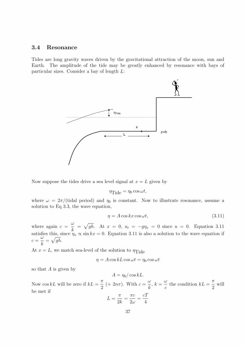
This result may be understood by considering the skater who with arms outstretched has aspin f and Q = f/h. As she brings her arms in her effective height increases. Now since herinitial and final potential vorticity remain the same

Qi =f

hi

= Qf =f + ζ

hf

and hf > hi we have an increase in her relative vorticity:

ζf

f=

hf

hi

− 1, (3.14)

i.e. she spins faster, (right hand rule). The same is also true for the fluid column sketched in

39

f f+

hi hf

Qi = f/hi = Qf = (f+ )/hf

Figure 3.5: Column squashing and stretching with rotation.

Figure 3.5 and cyclonic vorticity is acquired (ζ/f > 0) for vortex stretching and anticyclonicvorticity (ζ/f < 0) for vortex squashing: the column of fluid might be regarded as a vortex.

An Example : Geostrophic AdjustmentSuppose that water has been piled up against the coast as shown in Figure 3.6 but that thereis no motion. Now to infer the final sea-level and velocity field we expect that the waterwill move away from the coast (due to the pressure gradient), but that ultimately a sea-levelslope may exist that is in geostrophic balance

fv = gdη

dx

In addition we may consider the conservation of potential vorticity

Q =(ζ + f)

h(total)

of three columns (a), (b) and (c) as shown during the adjustment process and also note that

ζ =dv

dx

40

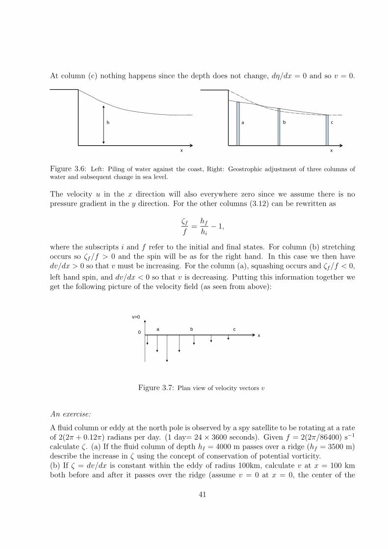
At column (c) nothing happens since the depth does not change, dη/dx = 0 and so v = 0.

h

x

a

x

b c

Figure 3.6: Left: Piling of water against the coast, Right: Geostrophic adjustment of three columns ofwater and subsequent change in sea level.

The velocity u in the x direction will also everywhere zero since we assume there is nopressure gradient in the y direction. For the other columns (3.12) can be rewritten as

ζf

f=

hf

hi

− 1,

where the subscripts i and f refer to the initial and final states. For column (b) stretchingoccurs so ζf/f > 0 and the spin will be as for the right hand. In this case we then havedv/dx > 0 so that v must be increasing. For the column (a), squashing occurs and ζf/f < 0,

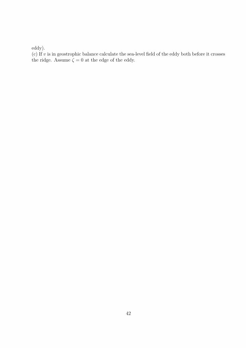
left hand spin, and dv/dx < 0 so that v is decreasing. Putting this information together weget the following picture of the velocity field (as seen from above):

v>0

0x

a b c

Figure 3.7: Plan view of velocity vectors v

An exercise:

A fluid column or eddy at the north pole is observed by a spy satellite to be rotating at a rateof 2(2π + 0.12π) radians per day. (1 day= 24× 3600 seconds). Given f = 2(2π/86400) s−1

calculate ζ. (a) If the fluid column of depth hI = 4000 m passes over a ridge (hf = 3500 m)describe the increase in ζ using the concept of conservation of potential vorticity.(b) If ζ = dv/dx is constant within the eddy of radius 100km, calculate v at x = 100 kmboth before and after it passes over the ridge (assume v = 0 at x = 0, the center of the

41

eddy).(c) If v is in geostrophic balance calculate the sea-level field of the eddy both before it crossesthe ridge. Assume ζ = 0 at the edge of the eddy.

42

4 Wind Forced Motions

The wind blowing on an ocean produces a force/unit area called a wind stress τ . The surfacewind stress can be related to the wind velocity through a relationship known as the ’bulkformula’.

(τx, τy) = ρaircDu10(ua, va) (4.1)

where τx and τy are respectively the zonal (x direction) and meridional (y direction) com-ponents of wind stress, cD is a bulk transfer coefficient for momentum (typically cD =1.5× 10−3), ρair is the density of air at the sea surface (∼ 1.3 kg m−3) and u10 is the speedof the wind at a height of 10 m above the ocean.

4.1 Ekman Layer

The effects of a wind stress on the ocean surface are transmitted down through the watercolumn by the action of turbulent eddies that are themselves generated by the wind, breakingwaves and boundary shear stresses. The depth to which the effects of wind are felt is calledthe Ekman layer thickness

HE = (2K/|f |) 12 (4.2)

where K is the eddy diffusivity and K ' WL where W and L denote a characteristic eddyvelocity and size. Typically K ' 2× 10−2 m2 s−1 so that with |f | = 10−4 s−1, HE ' 20 m.However in regions of high wind-driven turbulence, K can be up to 0.5 m2 s−1, so that He

can reach ' 100 m.

Now to understand the effects of wind consider the steady equations of motion for a barotropicocean of depth h. In the absence of wind and if the bottom stress is weak, these equationsof motion would be the geostrophic equations plus the effects of wind forcing, which thenenter as an extra frictional term, that is

−fv = −gdη

dx+

τx

ρh(4.3)

fu = −gdη

dy+

τy

ρh(4.4)

where τx and τy are the x− and y− direction components of the wind stress. Now for sim-plicity, let’s split the velocity field u and v into geostrophic and wind-driven components;that is:

u = ug + ue (4.5)

v = vg + ve (4.6)

43

where (ug, vg) denote geostrophic velocities such that there is a balance between the pressuregradient and the Coriolis force:

−fvg = −gdη

dx(4.7)

fug = −gdη

dy(4.8)

Hence the remainder of velocity (ue, ve) must balance the force of the wind:

−fve =τx

ρh(4.9)

fue =τy

ρh(4.10)

The velocities (ue, ve) are called the (depth-averaged) Ekman velocities and while drivenby the wind stress (τx, τy), the velocities (ue, ve) are at right angles to it.

4.2 The Ekman Velocity

To understand the effects of the wind let us assume it blows in the y direction only with aforce per unit area (a stress) denoted by τy. Assuming there are no sea level gradients, theequations of motion, averaged over the Ekman layer depth may be written as

dUE

dt− fVE = 0 (4.11)

dVE

dt+ fUE =

τy

ρHE

(4.12)

The horizontal velocity averaged over the Ekman layer is denoted by (UE, VE). Initially thereis no motion and the wind accelerates the column shown in Figure 4.1 in the y-directionaccording to dVE/dt = τy/ρHE.

As the column moves faster, the Coriolis force fVE gets larger and the column is deflectedto the right (Northern Hemisphere): dUE/dt = fVE. This continues until VE vanishes and asteady state is reached

fUE =τy

ρHE

(4.13)

and the Coriolis force and wind stress balance.The column moves at right angles to the wind.Hence the force balance on the fluid column is in this case between the Coriolis force andthe force of the wind.

44

VE

UE

fUE

fVE x

y

y/ HE

y

Figure 4.1: Plan view of the motion of a column of water subject to an initial accelerationby the wind.

An example:Calculate the Ekman velocity UE given a wind stress τy = 0.1 Pa (0.1 Nm−2) Assume anEkman layer depth of HE = 20 m, and f = 10−4 s−1 (Equation 4.13). Compare this to theconditions off northern California (Figure 4.6).

4.3 Depth Averaged Ekman Layer

Now to see what happens with depth we note that the wind only directly affects motionsover the depth He, not the entire depth h. Thus the velocity ue,ve only occurs in the Ekmanlayer and its value here must be (h/He) times the full depth-averaged velocity ue,ve. This iscalled the Ekman layer velocity and is given by

Ue =h

He

ue =τy

ρHef(4.14)

Ve =h

He

ve = − τx

ρHef(4.15)

since ue and ve represent velocity averaged over depth h. As shown in Figure 4.2, a north-south wind stress drives a velocity Ue in the east-west direction - that is, at right angles tothe wind. Checking the signs in Equations 4.14 and 4.15 we can see that flow is to the rightin the northern hemisphere, and to the left in the southern hemisphere.

45

Side View y

HE UE Ekman Layer

Figure 4.2: Side view of the movement of a column of water in the Ekman Layer in theNorthern Hemisphere. Note: There is no motion below the Ekman layer as there is no slopein sea level, hence the geostrophic velocities are zero.

An examplea) Find the Ekman layer depth He and the Ekman velocities ue and ve when a windof strength 0.5 Pascals (0.5 Newtons/m2) blows in a north-easterly direction in the mid-latitudes of the northern hemisphere. You can take the vertical diffusivity to be K = 0.1m2/ sec and f = 10−4 sec−1.b) What is the Ekman layer velocity Ue, Ve if the depth of the ocean h = 1000 m?c) Sketch the resultant flow.

4.4 Storm surges and Downwelling and Upwelling

4.4.1 Storm Surge

Let us now consider the effects of an alongshore wind stress on coastal circulation. Ourmodel is shown in Figure 4.3.

The effect of the coast is to block the onshore Ekman flux resulting in the raising of sea–level.Since η now changes with x, an alongshore geostrophic velocity

vg =g

f

dη

dx< 0

must exist to balance the force due to dη/dx.

Thus wind forcing results in the transport of water towards the coast in a thin layer HE,which can in turn raise sea–level and drive an alongshore velocity.

46

Sea level raised

Ue

Vg

τy

x

Figure 4.3: Idealised model of a storm surge (Northern Hemisphere).

4.4.2 Downwelling

Where the ocean is stratified (density increases with depth), the onshore Ekman flux alsopushes water down along the continental shelf leading to mixing and the growth of thickbottom boundary layers. The thermal wind shear near the shelf opposes, the alongshorecurrent vg = (g/f)dy/dx and an undercurrent flowing in the opposite direction can result.

Exercise: Use the thermal wind relation (2.18) and equation of state (2.10a) to show this isso.

UE

Inc.

Density

Vg

τy

Figure 4.4: Idealised downwelling scenario in the Northern Hemisphere.

47

4.4.3 Upwelling

Now consider the two–layer coastal model in Figure 4.5. With the wind stress directedinto the page the Ekman flux is directed off–shore so that the coastal sea–level must drop.However, we might expect the interface to rise as well and water (and nutrients) to be drawnfrom the deep ocean as shown.

Temp Decreases

Vg

τySea level is

lowered

Upwelling

Ue

Figure 4.5: Schematic diagram of wind driven upwelling in the Northern Hemisphere.

Ekman layer depths vary with wind forcing (strength and duration). An example is foundin the Northern Californian upwelling region during the WEST study (Largier et al., 2006;Roughan et al., 2006). Figure 4.6 from (Dever et al., 2006) shows data from a mooring in 90 mof water, showing along and across shelf wind (ms−1), temperature (C) and cross-shore andalong shore velocities throughout the water column. The coldest (warmest) temperaturescorrespond with the periods of strong (weak) alongshore wind forcing, and offshore (onshore)transport in the surface waters.

While coastal upwelling occurs in only about 1% of the oceans area, the increased biologicalproductivity accounts for about 50% of the worlds fish catch. Figure 4.7 shows the distri-bution of winds over the ocean, Note that the coast of Peru, west Africa and California aresubject to strong upwelling favourable winds.

48

E.P. Dever et al. / Deep-Sea Research II 53 (2006) 2887–2905

Figure 4.6: An example of upwelling favourable winds and the ocean response at the 90 misobath off the Northern Californian coast from (Dever et al., 2006). (A) along-shelf (solid)and cross-shelf (dashed) wind velocity, (B) temperature with surface and bottom mixedlayers (black lines), temperature logger depths (black triangles) (c) cross-shelf velocity withsurface and bottom mixed layers (black lines), and Pollard Rhines and Thompson scaling(magenta lines) and (D) along-shelf velocity with surface and bottom mixed layers (blacklines).

4.5 Ekman Pumping

In the above we have implicitly assumed that the wind stress τy and thus Ekman flux UE

are constant. What if τy changes in space (e.g with x). In the schematic in Figure 4.8 it isapparent that the flux UE will converge at the origin leading to a flux of water wE out ofthe Ekman layer. The velocity wE is called the Ekman pumping velocity and given by

wE(z = HE) = −HEdUE

dx(4.16)

49

Figure 4.7: Map showing the annual mean distribution of winds around the world. Whichregions are upwelling favourable?

y

UE UE

WE

x

z

Figure 4.8: Ekman Pumping, resulting from a curl (change) in the wind stress.

50

or

wE = − d

dx(τy/ρf) (4.17)

It corresponds to a velocity of fluid leaving or entering the base of the Ekman layer so as tocompensate the horizontal variations in the horizontal flow due to the Ekman flux UE.

An example: a hurricaneConsider the single layer ocean in Figure 4.9 that is subject to the wind stress field shown(a hurricane).

x

z

V

We

UeUe

τy τy

Figure 4.9: Schematic Diagram of the sea surface response to a Hurricane . Note that theEkman layer thins leading to vortex stretching of the lower layer (ζ/f ≥ 0).

For the northern hemisphere UE is directed to the right of the wind τ so that there is a lossof fluid in the Ekman layer. However, this fluid is replaced by the upward Ekman pumpingvelocity wE. Note that not all the fluid is replaced and we might expect sea–level to dip inthe centre as shown.

51

Figure 4.10: Two sections showing isopycnals as observed several days after the passage ofa Hurricane across the Gulf of Mexico. The offshore Ekman transport and resultant Ekmanupwelling has raised the isopycnals by more than 60 m near the hurricane center.

ExerciseUse the thermal wind relations to estimate the change in velocity over a depth of 80−100 mat the position indicated by the arrow for section C-C‘.

4.6 Circulation along the Equator

There is a complicated current structure near the equator which is associated with the winddriven circulation in each hemisphere. The North and South Equatorial Currents (NECand SEC) are westward currents that are associated with the wind gyres with speeds of25 − 30 cms−1 and 50 − 65 cms−1 respecitively, (the SEC is larger due to stronger tradewinds in the south). In addition, an eastward North Equatorial Counter–Current (NECC)exists in the region of the doldrums, (4− 10N). It is highly variable 35− 60 cms−1 and canextend to 1500 m in depth. To understand these currents, consider the Ekman transport,

52

Latitude

0 4 10

Doldrums

WE

VE

VE

VE

τx

South North

WE

WE

η

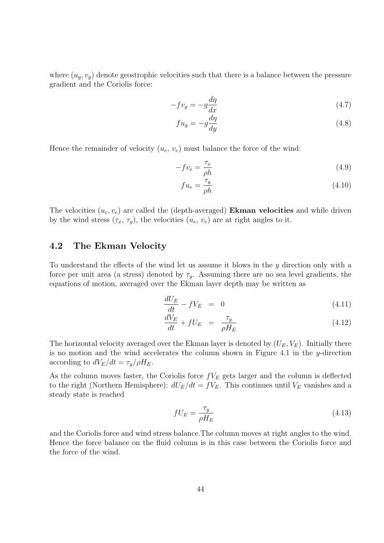
Figure 4.11: Schematic diagram showing the circulation in the Equatorial Pacific

VE =−τx

ρfHE

The SE trades create a southward Ekman transport in the southern hemisphere but a north-ward transport between 0−4N since f changes sign. In addition from 10S to the Equator,the sea level is lowered and the thermocline is raised. North of the equator sea level risesbecause τx ' 0 in the doldrums. Further north the winds again blow to the west and againsea level is raised by the Ekman transport. Geostrophy leads to the observed NECC andthe intensification of the SEC and NEC that are associated with the wind driven gyre.

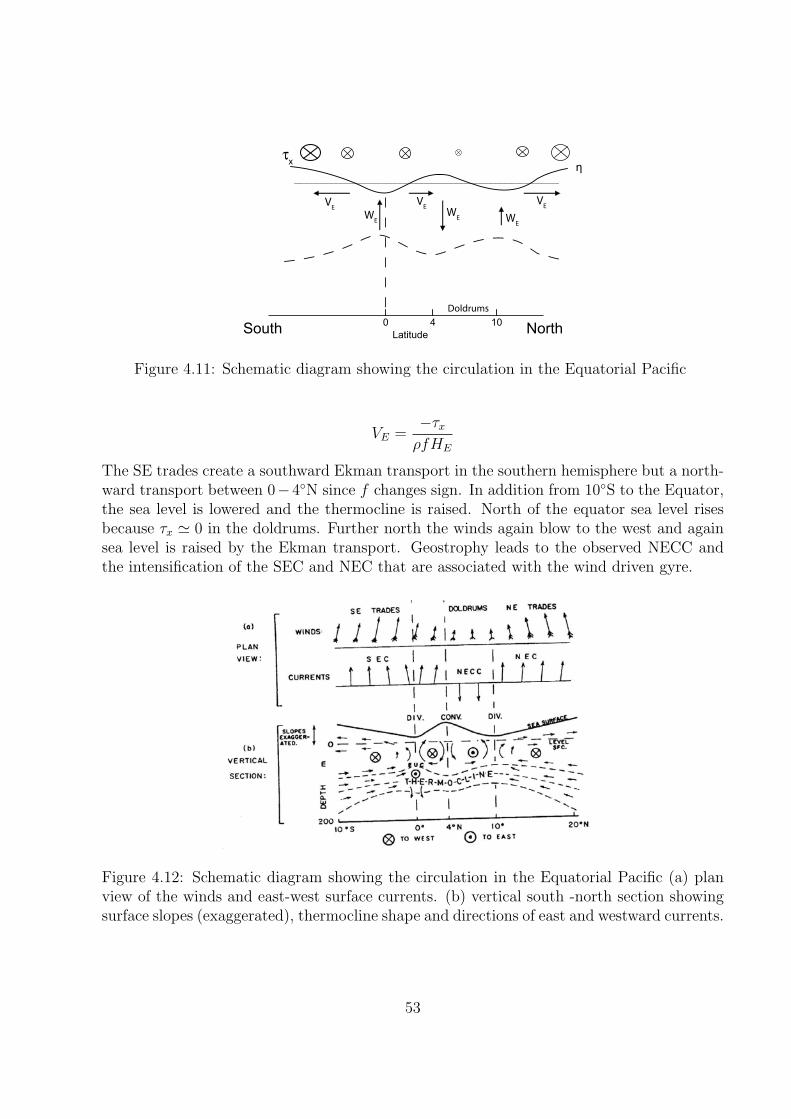
Figure 4.12: Schematic diagram showing the circulation in the Equatorial Pacific (a) planview of the winds and east-west surface currents. (b) vertical south -north section showingsurface slopes (exaggerated), thermocline shape and directions of east and westward currents.

53

An additional feature is the Equatorial Undercurrent, some 300 km wide and 200m deepextending across the Pacific (14, 000 km) with speeds of up to 1.7 ms−1 and transport of40 Sv.

Figure 4.13: Cross sections of temperature, salinity, oxygen, phosphate and velocity at 140oWin the Pacific. In the mixed layer above the thermocline, the water is high in oxygen and lowin phosphate. The reverse is true below. Tongues of high salinity extend equatorward. Theslope of the thermocline is consitent with a north and south equatorial current separated by acounter current between 5−10N (confined to the mixed layer). The Equatorial Undercurrentand its effect on the thermocline can be seen at the equator. From Knauss (2000).

The current arises from the westward wind and blocking due to the islands in the WesternPacific. With x− in the directed eastward the barotropic momentum equation is given by

du

dt− fv = −g

dη

dx+

τx

ρh− ru

h.

54

Right at the equator f = 0 and if the flow does not accelerate du/dt = 0 so that

dη

dx=

τx

ρgh− ru

gh(4.18)

and water is piled up in the west by the wind. A flow u to the east exists which acts to drainthis reservoir of water: the flow is the Equatorial Undercurrent.

The model (Equation 4.18) makes no allowance for how things vary with depth. Within thesurface Ekman layer, the current is in the direction of the wind

ru ' τx

ρ< 0

Below this layer, the direct effects of the wind vanish and the Undercurrent is driven by thesea level gradient:

ru

gh' −dη

dx> 0

At depths of more than 300 m, the thermal wind effect due to the depressed isotherms inthe western Pacific, cancels out the pressure gradient due to the sea level. The Undercurrentvanishes.

Figure 4.14: Velocity (left) and temperature (right) transect through the equatorial under-current. A doming in the isotherms is associated with the eastward flowing undercurrent.

Away from the equator f is non-zero so that a north-south current v may exist. However,north of the equator f > 0 so that the geostrophic current vs = (g/f) dη/dx is negative sincedη/dx is also. Thus, the geostrophic current would tend to push the EUC back along theequator. A similar argument applies to the velocity vg south of the equator.

55

Figure 4.15: a) west-east section along the equator of thermosteric anomaly (b,c) Schematicof south-north sections across currents in the western and eastern Pacific (d) south-northsection for salinity in west (e) Schematic of south - north section for temperature in the east.Pond and Pickard (1983)

56

5 Meridional Circulation in the Atmosphere

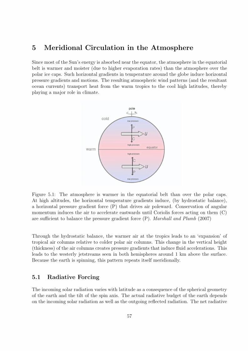
Since most of the Sun’s energy is absorbed near the equator, the atmosphere in the equatorialbelt is warmer and moister (due to higher evaporation rates) than the atmosphere over thepolar ice caps. Such horizontal gradients in temperature around the globe induce horizontalpressure gradients and motions. The resulting atmospheric wind patterns (and the resultantocean currents) transport heat from the warm tropics to the cool high latitudes, therebyplaying a major role in climate.

Figure 5.1: The atmosphere is warmer in the equatorial belt than over the polar caps.At high altitudes, the horizontal temperature gradients induce, (by hydrostatic balance),a horizontal pressure gradient force (P) that drives air poleward. Conservation of angularmomentum induces the air to accelerate eastwards until Coriolis forces acting on them (C)are sufficient to balance the pressure gradient force (P). Marshall and Plumb (2007)

Through the hydrostatic balance, the warmer air at the tropics leads to an ‘expansion’ oftropical air columns relative to colder polar air columns. This change in the vertical height(thickness) of the air columns creates pressure gradients that induce fluid accelerations. Thisleads to the westerly jetstreams seen in both hemispheres around 1 km above the surface.Because the earth is spinning, this pattern repeats itself meridionally.

5.1 Radiative Forcing

The incoming solar radiation varies with latitude as a consequence of the spherical geometryof the earth and the tilt of the spin axis. The actual radiative budget of the earth dependson the incoming solar radiation as well as the outgoing reflected radiation. The net radiative

57

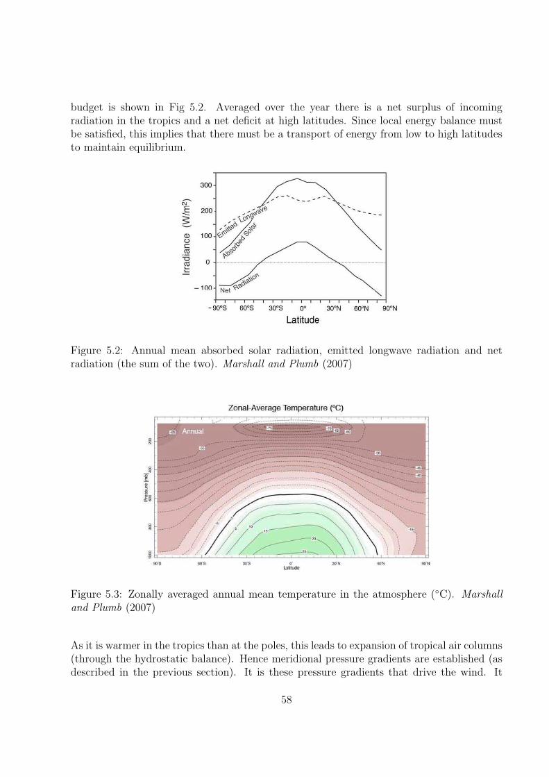
budget is shown in Fig 5.2. Averaged over the year there is a net surplus of incomingradiation in the tropics and a net deficit at high latitudes. Since local energy balance mustbe satisfied, this implies that there must be a transport of energy from low to high latitudesto maintain equilibrium.

Figure 5.2: Annual mean absorbed solar radiation, emitted longwave radiation and netradiation (the sum of the two). Marshall and Plumb (2007)

Figure 5.3: Zonally averaged annual mean temperature in the atmosphere (C). Marshalland Plumb (2007)

As it is warmer in the tropics than at the poles, this leads to expansion of tropical air columns(through the hydrostatic balance). Hence meridional pressure gradients are established (asdescribed in the previous section). It is these pressure gradients that drive the wind. It

58

is customary in meteorology to use pressure rather than height as the primary vertical co-ordinate. Since in hydrostatic balance, pressure is directly related to the overlying massburden, pressure is actually a mass co-ordinate. In observations it is simpler to measurepressure in situ rather than height. The height of a given pressure surface is dependent onthe average temperature below that surface and the surface pressure :

z(p) = R

∫ ps

p

T

g

dp

p(5.1)

As tropical air columns are warmer than polar columns at all levels, then the pressure tiltmust increase with height as in Figure 5.4.

Figure 5.4: Warm columns of air expand, cold columns of air contract, leading to a tilt ofpressure surfaces, which typically increases with height in the tropopshere. Correspondingwinds are out of the page. Marshall and Plumb (2007)

It is also useful to define the thickness of an atmospheric layer, between two pressure surfacessuch as p1 and p2, e.g. in Figure 5.4. We have

z2 − z1 = R

∫ p1

p2

T

g

dp

p(5.2)

which depends on T averaged over the layer. Atmospheric layers are ‘thick’ in tropicalregions because they are warm and ‘thin’ in polar regions because they are cold, leading tothe large-scale slope of pressure surfaces.

59

Figure 5.5: MSLP (solid) and 1000 to 500 hPa thickness (dashed) chart for Australia. The5400 thickness line (rule of thumb: snow > 1800 m) has penetrated well north over thesoutheast mainland in cold southwest winds behind a cold front over the Tasman Sea. Thisbrought widespread snow to the NSW and Victorian Alps.

5.2 The Hadley Cell

As tropical air columns are warmer than polar columns at all levels there is thus a pressuregradient aloft directed from high pressure to low pressure, i.e from warm latitudes to coldlatitudes. Hadley (1735) suggested that there was one giant meridional cell with rising motionin the tropics and descending motion at the poles. This explanation is a little simplified,and the circulation is more complex.

Since most of the Sun’s energy is absorbed near the equator, we expect greater heating of theatmosphere. This heating results in a Hadley cell whereby the warmed air rises, up to 12 kmnear the equator, is transported towards the poles and then sinks (at latitudes ∼ 20− 30).This Hadley cell helps to transport the heat towards the colder poles resulting in a moreuniform temperature distribution than would otherwise be the case. In addition, the celldrives the westward (easterly) trade winds near the ocean surface.

60

Figure 5.6: Meridional overturning streamfunction (χ) of the atmosphere in annual mean,(top) DJF (middle) JJA (bottom). Units are in 109 kg s−1 . Flow circulates around positive(negative) centres in a clockwise (anti-clockwise) sense. Thus in the annual mean, air risesjust north of the equator and sinks around ±30. Marshall and Plumb (2007)

A simple model for the Hadley cell can be obtained from our equations of motion and froman additional equation for density. This equation may be written as

∂p

∂t= −w

∂ρ

∂z︸ ︷︷ ︸(i)

− ρ0Q︸︷︷︸(ii)

−α(ρ− ρ0)︸ ︷︷ ︸

(iii)

(5.3)

which states that density may change due to 3 factors. The first term (i) involves changes

61

in density due to the vertical advection (or transport of density). If ρ does not change with

height (−z), then∂ρ

∂t= −w

∂ρ

∂z= 0. No change in density. However, suppose that ρ is larger

near the Earth’s surface (z ' 0). In this case∂ρ

∂z> 0 and if w < 0 (upwards motion) then

∂ρ

∂t= −w

∂ρ

∂z> 0 (5.4)

That is the vertical transport of relatively dense air will increase the density above and∂ρ

∂t> 0.

The second term (ii) involves the effect of heating by the long and short waves, and we willassume it can be modelled by

Q = −Q0 cos(`y) sin(mz) (5.5)

where ` =π

Land m =

π

D. For Q0 > 0, this term will heat and cool the air (make less and

more dense). The third term (iii) is called Newtonian cooling and acts to make the densityρ return to some basic state p0(z) in the absence of any other effects.

∂ρ

∂t= −α(ρ− ρ0). (5.6)

Using the following decomposition for density ρ = ρ0(z) + ρ′(x, y, z, t), the above may bewritten as

∂ρ′

∂t= −αρ′

so if ρ′ ≡ ρ at time zeroρ′ = ρ exp(−αt)

and in analogy with friction, ρ′ collapses to zero with an e-folding time scale equal to1

α.

Now collecting the above, Equation 5.3 may be re-written as

1

ρ0

∂ρ′

∂t= −Bw −Q− αρ′

ρ0

(5.7)

where B =1

ρ0

∂ρ0

∂zis assumed constant. Our x-momentum equation is

∂u

∂t= fv −Ru (5.8)

where R−1 is the e-folding time scale for friction. No pressure forces are allowed in the x(west) direction. Our y-momentum equation is

∂v

∂t= −fu− 1

ρ0

∂p′

∂y−Rv (5.9)

62

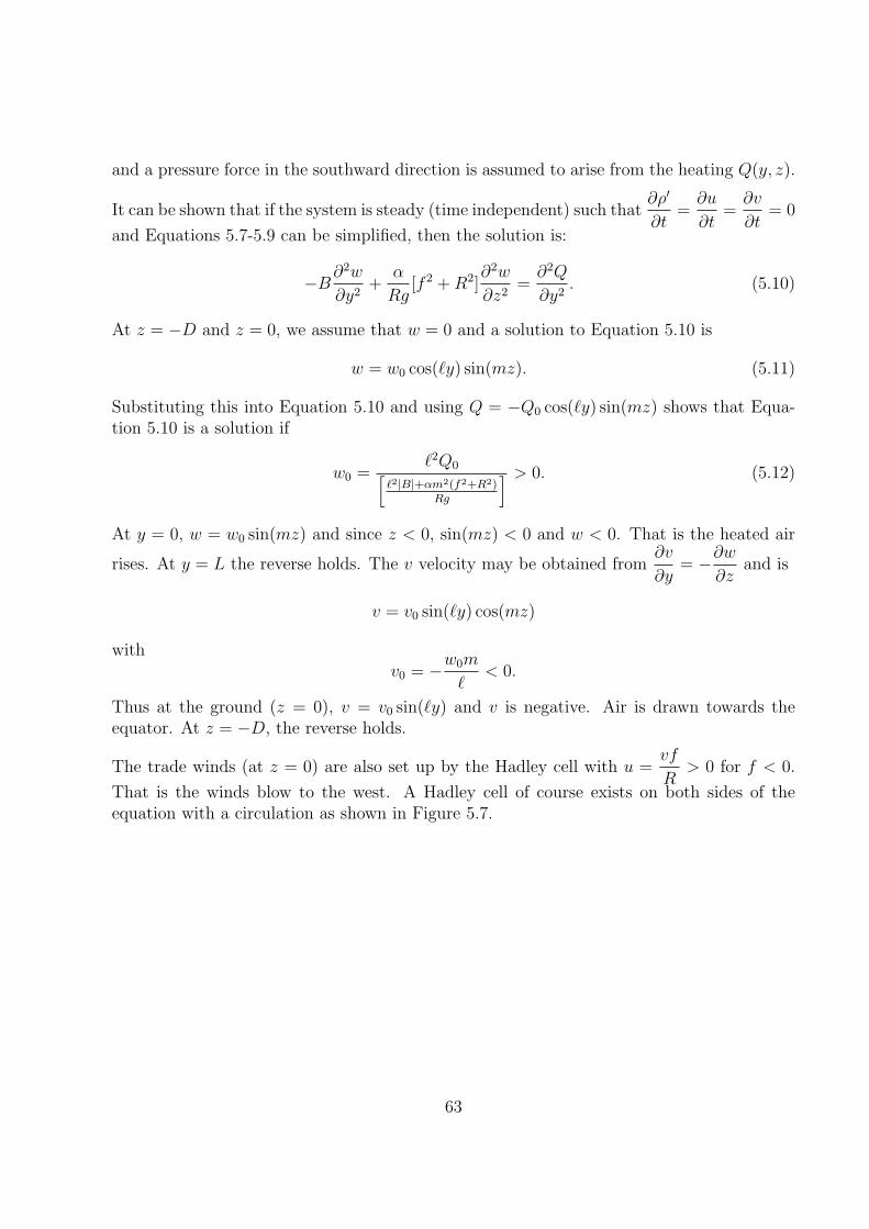
and a pressure force in the southward direction is assumed to arise from the heating Q(y, z).

It can be shown that if the system is steady (time independent) such that∂ρ′

∂t=

∂u

∂t=

∂v

∂t= 0

and Equations 5.7-5.9 can be simplified, then the solution is:

−B∂2w

∂y2+

α

Rg[f 2 + R2]

∂2w

∂z2=

∂2Q

∂y2. (5.10)

At z = −D and z = 0, we assume that w = 0 and a solution to Equation 5.10 is

w = w0 cos(`y) sin(mz). (5.11)

Substituting this into Equation 5.10 and using Q = −Q0 cos(`y) sin(mz) shows that Equa-tion 5.10 is a solution if

w0 =`2Q0[

`2|B|+αm2(f2+R2)Rg

] > 0. (5.12)

At y = 0, w = w0 sin(mz) and since z < 0, sin(mz) < 0 and w < 0. That is the heated air

rises. At y = L the reverse holds. The v velocity may be obtained from∂v

∂y= −∂w

∂zand is

v = v0 sin(`y) cos(mz)

withv0 = −w0m

`< 0.

Thus at the ground (z = 0), v = v0 sin(`y) and v is negative. Air is drawn towards theequator. At z = −D, the reverse holds.

The trade winds (at z = 0) are also set up by the Hadley cell with u =vf

R> 0 for f < 0.

That is the winds blow to the west. A Hadley cell of course exists on both sides of theequation with a circulation as shown in Figure 5.7.

63

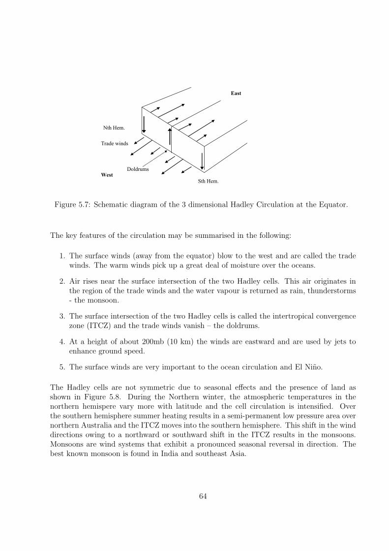
East

Nth Hem.

Trade winds

Doldrums

West

Sth Hem.

Figure 5.7: Schematic diagram of the 3 dimensional Hadley Circulation at the Equator.

The key features of the circulation may be summarised in the following:

1. The surface winds (away from the equator) blow to the west and are called the tradewinds. The warm winds pick up a great deal of moisture over the oceans.

2. Air rises near the surface intersection of the two Hadley cells. This air originates inthe region of the trade winds and the water vapour is returned as rain, thunderstorms- the monsoon.

3. The surface intersection of the two Hadley cells is called the intertropical convergencezone (ITCZ) and the trade winds vanish – the doldrums.

4. At a height of about 200mb (10 km) the winds are eastward and are used by jets toenhance ground speed.

5. The surface winds are very important to the ocean circulation and El Nino.

The Hadley cells are not symmetric due to seasonal effects and the presence of land asshown in Figure 5.8. During the Northern winter, the atmospheric temperatures in thenorthern hemispere vary more with latitude and the cell circulation is intensified. Overthe southern hemisphere summer heating results in a semi-permanent low pressure area overnorthern Australia and the ITCZ moves into the southern hemisphere. This shift in the winddirections owing to a northward or southward shift in the ITCZ results in the monsoons.Monsoons are wind systems that exhibit a pronounced seasonal reversal in direction. Thebest known monsoon is found in India and southeast Asia.

64

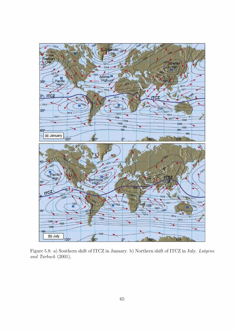
Figure 5.8: a) Southern shift of ITCZ in January. b) Northern shift of ITCZ in July. Lutgensand Tarbuck (2001),

65

5.3 Ferrel Cells

5.4 Monsoons

5.5 Trade Winds

5.6 Baroclinic Instability: Highs and Lows

The weather at midlatitudes (40-50 degrees) is dominated by the presence of high and lowpressure systems as exemplified by the figure below. What causes these pressure systemsand what role do they play in the global redistribution of heat?

Figure?

To answer this question (in part) consider the idealised northern hemisphere model sketchedbelow. The atmosphere is cooled by the interior cylinder and heated at the outer cylinder.The interior cooling causes the air to become dense, descend and be deflected to the rightas shown. Along the outer cylinder the reverse holds and the air is deflected to the west. Inaddition, the density field changes as indicated with colder air to the north.

After some time, a thermal wind balance is set up

∂v

∂z=

(g

ρ0f

)∂σ

∂x

and near the top of the atmosphere, the thermal wind blows in the same direction as therotating Earth. That is, from west to east. This wind is called the jet stream and is strongestin the northern hemisphere due to the presence of the land masses which accentuate thetemperature difference between north and south. In the southern hemisphere, the presenceof the Atlantic, Pacific and Southern Oceans moderate temperature difference.

66

Figure?∂v

∂z=

g

ρ0f

∂σ

∂x< 0

The high and low pressure systems result from a process known as baroclinic instability.The energy for this instability (and the pressure systems) comes from the tilted density field(shown above) that results from the cooling and heating. The instability, illustrated below,“feeds” on this energy and the resultant high and low systems act to transport heat awayfrom the equator and towards the poles.

5.7 The Sea Breeze

The afternoon sea breeze is caused by the differential heating by land and sea that can bequite strong during summer. The warmer land acts to heat the air above the land leadingto lighter air and low in pressure. The denser, cooler air over the ocean slides under andtowards the land resulting in the breeze. The vertical motion associated with the breeze isalso effected by the change in the density of air.

Figure?

Over the land, the hydrostatic balance does not hold. Rather, since the air is less dense, the

upwards pressure force1

ρ

dp

dzexceeds that due to gravity g and

dw

dt=

1

ρ

dp

dz+ g < 0,

so that w is negative (rising air). Over the sea the reverse holds.

67

References

Cushman-Roisin, B., and J. Beckers (2007), Introduction to Geophysi-cal Fluid Dynamics Physical and Numerical Aspects, Prentice Hall Inc.,http://engineering.dartmouth.edu/ cushman/books/GFD.html.

Dever, E. P., C. E. Dorman, and J. L. Largier (2006), Surface boundary layer vari-ability off northern California, USA during upwelling, Deep-Sea Res., 53, 2887–2905,doi:10.1016/j.dsr2.2006.09.001.

Knauss, J. A. (2000), Introduction to Physical Oceanography, Prentice Hall.

Largier, J. L., C. Lawerence, M. Roughan, D. Kaplan, E. Dever, C. Dorman, R. Kudela,S. Bollens, F. Wilkerson, R. Dugdale, L. Botsford, N. Garfield, B. Kuebel-Cervantes, andD. Koracin (2006), West a northern California study of the role of wind-driven trans-port in the productivity of coastal plankton communities, Deep-Sea Res., 53, 2833–2849,doi:10.1016/j.dsr2.2006.08.018.

Lutgens, and Tarbuck (2001), The Atmosphere, Prentice Hall.

Marshall, J., and A. Plumb (2007), Circulation of the Atmosphere and Ocean: An introduc-tory text., Massachusetts Institute of Technology.

Olson, D. B. (1980), The physical oceanography of two rings observed by the cyclonic ringexperiment. part 2 dynamics., J. Phys. Oceanogr., 10, 514–528.

Olson, D. B. (1991), Rings in the ocean, Annu. Rev. Earth Panet. Sci., 19, 283–311.

Pond, S., and G. L. Pickard (1983), Introductory Dynamical Oceanography, Pergamon Press.

Roughan, M., N. Garfield, J. Largier, E. Dever, C. Dorman, D. Peterson, and D. J. (2006),Transport and retention in an upwelling region: the role of across-shelf structure., Deep-Sea Res., 53, 2931–2955, doi:10.1016/j.dsr2.2006.07.015.

Thurman, H. V., and E. A. Burton (2001), Introductory Oceangography, 9th ed., PrenticeHall.

68